TGNN: A Joint Semi-Supervised Framework for Graph-Level Classification

Abstract

This paper studies semi-supervised graph classification, a crucial task with a wide range of applications in social network analysis and bioinformatics. Recent works typically adopt graph neural networks to learn graph-level representations for classification, failing to explicitly leverage features derived from graph topology (e.g., paths). Moreover, when labeled data is scarce, these methods are far from satisfactory due to their insufficient topology exploration of unlabeled data. We address the challenge by proposing a novel semi-supervised framework called Twin Graph Neural Network (TGNN). To explore graph structural information from complementary views, our TGNN has a message passing module and a graph kernel module. To fully utilize unlabeled data, for each module, we calculate the similarity of each unlabeled graph to other labeled graphs in the memory bank and our consistency loss encourages consistency between two similarity distributions in different embedding spaces. The two twin modules collaborate with each other by exchanging instance similarity knowledge to fully explore the structure information of both labeled and unlabeled data. We evaluate our TGNN on various public datasets and show that it achieves strong performance.

1 Introduction

A fundamental problem in data mining is graph classification, which seeks to capture the property of the entire graph. The problem has been extensively studied lately with a range of downstream applications, such as predicting the quantum mechanical properties Lu et al. (2019); Hao et al. (2020) and assessing the functionality of chemical compounds Kojima et al. (2020). Among various graph classification algorithms Ying et al. (2018); Xu et al. (2019), message-passing neural networks (MPNNs), as the majority of graph neural networks (GNNs) Kipf and Welling (2017); Veličković et al. (2017), have achieved tremendous success. The main idea behind MPNNs is to propagate and aggregate messages on a graph Gilmer et al. (2017), where each node receives messages from all its neighbors, and then iteratively performs neighborhood aggregation and node updates. Finally, all node representations can be combined into a graph-level representation. In this way, the semantic knowledge of local structures represented by different nodes can be implicitly integrated into the graph-level representation.

Although GNNs have achieved impressive performance, they do have one drawback that optimizing effective GNNs is data-hungry and frequently relies on a large number of labeled graphs, as the settings of current graph classification tasks show Xu et al. (2019). Nevertheless, it is often expensive and time-consuming to annotate labels such as in biochemistry and chemistry Hao et al. (2020). Although the labeled samples could be limited, massive unlabeled samples are simple to obtain, whose structures can often regularize the graph encoder to learn more discriminative representations for classification. This thus naturally inspires us to leverage both labeled and unlabeled data in semi-supervised scenarios to address the limitations of existing methods.

Recent efforts of combining MPNNs with semi-supervised learning techniques for graph classification Li et al. (2019); Sun et al. (2020); Hao et al. (2020); Luo et al. (2022) are usually divided into two categories: self-training Lee and others (2013) or knowledge distillation Hinton et al. (2014). However, topology information is only implicitly incorporated when node features are messaging along edges, which fails to effectively explore graph topology. Moreover, as the number of labeled graphs is limited in semi-supervised graph classification, an approach that can better model graph topology and explore the unlabeled data for classification is anticipated in real-world applications.

To address the above issues, we propose a new framework named TGNN, which is capable of better exploring graph structures for semi-supervised graph-level classification. In contrast to existing MPNNs which utilize graph structures in an implicit way via message passing, our approach aims to capture graph topology in both implicit and explicit manners. On the one hand, we follow MPNNs and learn structured node representations through neighbor aggregation, and the summarized graph representation implicitly captures graph topology. On the other hand, we employ a graph kernel module, which compares each graph with parameterized hidden graphs via the random walk kernel. By this means, we get another graph representation, which leverages graph topology more explicitly. In order to couple the explicit and implicit information of graph topology, we propose a unified semi-supervised optimization framework with a novel self-supervised consistency loss, where two modules are encouraged to yield consistent similarity scores when applied to each unlabeled graph. Extensive experiments on a wide range of well-known graph classification datasets demonstrate significant improvements over competing baselines. The contributions of this work can be summarized as follows:

• We provide a new semi-supervised graph classification approach called TGNN, which comprises a message passing module and a graph kernel module to explore structural information in both implicit and explicit ways.

• To integrate the topology information from complementary views, we propose an optimization framework including a self-supervised consistency loss to encourage exchanging similarity knowledge between two modules.

• Experimental results show our TGNN significantly outperforms the compared baselines by a large margin on a variety of benchmark datasets.

2 Related Work

Graph Neural Networks. GNNs have been extensively investigated due to their simplification from spectral methods Spielman (2007) to localized models Kipf and Welling (2017), which connects GNNs to message passing framework Gilmer et al. (2017) and significantly promotes its efficiency. Most existing GNN methods for graph classification task Hao et al. (2020); Ju et al. (2022) inherently use message passing neural networks (MPNNs) Gilmer et al. (2017) to learn graph-level representation. However, MPNNs bear the drawback that they ignore structural properties explicitly emanating from graph topology. Furthermore, recent studies have shown the inability of MPNNs to model high-order substructures such as paths Chen et al. (2020); Long et al. (2021). With our TGNN, besides implicitly learning effective graph structural information from MPNNs, we also benefit from the graph kernel module to explicitly incorporate graph topology in a semi-supervised framework.

Semi-supervised Graph Classification. Semi-supervised learning has attracted increasing attention in the field of machine learning and data mining Grandvalet and Bengio (2005); Laine and Aila (2017); Tarvainen and Valpola (2017), whose basic idea is effectively leveraging a small number of labeled data and massive available unlabeled data to enhance the model performance. Recently much work has been done for semi-supervised graph classification Li et al. (2019); Sun et al. (2020); Hao et al. (2020); Luo et al. (2022). SEAL-AI Li et al. (2019) and ASGN Hao et al. (2020) use active learning techniques to select the most representative samples from unlabeled data, while InfoGraph Sun et al. (2020) and DualGraph  Luo et al. (2022) fully explore the semantic information of unlabeled data via contrastive learning. Different from existing methods which only model graph topology in an implicit way, we also consider structural information in an explicit manner via graph kernels.

3 Methodology

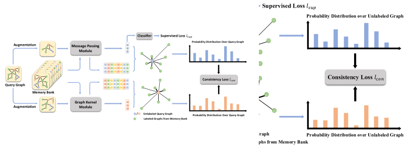
Figure 1: The schematic of the proposed framework TGNN. Our TGNN is a joint framework with twin GNNs (i.e., a message passing module and a graph kernel module), which is trained by minimizing the supervised loss as well as self-supervised consistency loss based on graph representations in two kinds of embedding spaces.

This paper provides a novel framework TGNN for semi-supervised graph classification as shown in Figure 1. At a high level, TGNN aims to capture graph topology in both implicit and explicit manners with twin GNN modules. On the one hand, we follow MPNNs to learn structured node representations via message passing, and thus the summarized graph representation reflects graph topology implicitly. On the other hand, we introduce a graph kernel module, which compares each unlabeled graph with hidden graphs via a random walk kernel to explicitly explore graph topology. To couple different topology information from twin GNNs, we present a novel semi-supervised optimization approach, in which twin modules are enforced to yield consistent similarity scores when applied to each unlabeled graph.

Problem Definition. Let $G=(V,E)$ denote a graph, where $V$ and $E$ represent the node set and the edge set, respectively. In the task of semi-supervised graph classification, we are given a whole graph set $\mathcal{G}=\{\mathcal{G}^{L},\mathcal{G}^{U}\}$, which contains labeled graphs $\mathcal{G}^{L}=\left\{G_{1},\cdots,G_{\left|\mathcal{G}^{L}\right|}\right\}$ with their labels $\mathcal{Y}^{L}=\{y_{1},\cdots,y_{\left|\mathcal{G}^{L}\right|}\}$ and unlabeled graphs $\mathcal{G}^{U}=$ $\left\{G_{\left|\mathcal{G}^{L}\right|+1},\cdots,G_{\left|\mathcal{G}^{L}\right|+\left|\mathcal{G}^{U}\right|}\right\}$. We aim to learn a label distribution $p(\mathcal{Y}^{U}|\mathcal{G},\mathcal{Y}^{L})$, which is able to predict the categories for unlabeled graphs $\mathcal{G}^{U}$.

3.1 Message Passing Module

Message passing neural networks (MPNNs)  Kipf and Welling (2017); Gilmer et al. (2017); Veličković et al. (2017) have recently emerged as promising approaches to model graph-structured data, which implicitly encode graph structure into learned node representations $\mathbf{h}_{v}^{(k)}$ for each node $v$ at the $k$-th layer. MPNNs typically use neighborhood aggregation to iteratively update the representation of a node by incorporating representations of its neighboring nodes in the previous layer. After $k$ iterations, a node representation $\mathbf{h}_{v}^{(k)}$ is able to capture the structural information within its $k$-hop neighborhoods. Formally, the $k$-th layer of a node representation $\mathbf{h}_{v}^{(k)}$ obtained from the MPNN is formulated as:

$$\mathbf{h}_{v}^{(k)}=\operatorname{COM}^{(k)}_{\theta}\left(\mathbf{h}_{v}^{(k-1)}+\sum_{u\in\mathcal{N}(v)}\mathbf{h}_{u}^{(k-1)}\right)$$ (1)

Here $\mathcal{N}(v)$ represents the set neighbors of node $v$, $\operatorname{COM}^{(k)}_{\theta}$ is a non-linear combination operations at layer $k$. Eventually, by using an attention mechanism, the graph-level representation will be generated by integrating all node representations at layer $K$ as follows:

$$f_{\theta}\left(G\right)=\sum_{v\in V}a_{v}\mathbf{h}_{v}^{(K)}$$ (2)

$$a_{v}=\frac{\text{exp}(\mathbf{t}^{\top}\mathbf{h}_{v}^{(K)})\mathbb{I}_{\mathbf{t}^{\top}\mathbf{h}_{v}^{(K)}>0}}{\sum_{v\in V}\text{exp}(\mathbf{t}^{\top}\mathbf{h}_{v}^{(K)})\mathbb{I}_{\mathbf{t}^{\top}\mathbf{h}_{v}^{(K)}>0}}$$ (3)

where $\mathbf{t}$ is a learnable vector, $f_{\theta}\left(G\right)$ is the graph-level representation, and $\theta$ denotes the parameters of the message passing module. $\mathbb{I}_{(\cdot)}$ is an indicator equaling 1 when the condition is met, and its introduction is to adaptively prune some unimportant nodes for discriminative graph-level representations.

3.2 Graph Kernel Module

However, recent MPNNs simply capture structural information implicitly via message-passing along edges. It is usually difficult to explore rich high-order substructures (e.g., paths Chen et al. (2020); Long et al. (2021)) in various MPNN models. It is therefore desirable to have a principled way of incorporating structural information explicitly.

To this end, we propose to use a random walk graph kernel to explicitly explore graph topology. Our graph kernel module introduces some hidden graphs which are parameterized using trainable adjacency matrices. Formally, our module contains $N$ hidden graphs $G^{\prime}_{1},G^{\prime}_{2},\cdots,G^{\prime}_{N}$ with different sizes. We parametrize each hidden graph $G^{\prime}_{i}$ as an undirected graph for fewer parameters. These hidden graphs are expected to learn structures that help distinguish between available classes. Inspired by the fact that the random walk kernels quantify the similarity of two graphs based on the number of common walks in the two graphs Kashima et al. (2003); Nikolentzos and Vazirgiannis (2020), we compare each graph sample against hidden graphs with a differentiable function from the random walk kernel.

Specifically, given two graphs $G=(V,E)$ and $G^{\prime}=(V^{\prime},E^{\prime})$, their graph direct product $G_{\times}=(V_{\times},E_{\times})$ is a graph where $V_{\times}=\left\{\left(v,v^{\prime}\right):v\in V\wedge v^{\prime}\in V^{\prime}\right\}$ and $E_{\times}=\left\{\left\{\left(v,v^{\prime}\right),\left(u,u^{\prime}\right)\right\}:\{v,u\}\in E\wedge\left\{v^{\prime},u^{\prime}\right\}\in E^{\prime}\right\}$. It could be observed that a random walk on $G_{\times}$ can be interpreted as a simultaneous walk on graphs $G$ and $G^{\prime}$ Vishwanathan et al. (2010). Considering traditional random walk kernels count all pairs of matching walks on $G$ and $G^{\prime}$, the number of matching walks is equivalent to the adjacency matrix $\mathbf{A}_{\times}$ of $G_{\times}$ if traversing over nodes of $G$ and $G^{\prime}$ at random. The $P$-step ($P\in\mathbb{N}$) random walk kernel between $G$ and $G^{\prime}$ that counts all simultaneous random walks is thus defined as:

$$k\left(G,G^{\prime}\right)=\sum_{p=0}^{P}\omega_{p}\mathbf{e}^{\top}\mathbf{A}_{\times}^{p}\mathbf{e}$$ (4)

where $\mathbf{e}$ is an all-one vector, and $\omega_{0},\dots,\omega_{P}$ are positive weights. To simplify the calculation, we only compute the number of common walks of length exactly $p$ over two compared graphs:

$$k^{(p)}\left(G,G^{\prime}\right)=\mathbf{e}^{\top}\mathbf{A}_{\times}^{p}\mathbf{e}$$ (5)

Then, given $\mathcal{P}=\{0,\dots,P\}$ and hidden graph set $\mathbf{\mathcal{G}}_{h}=\{G^{\prime}_{1},\dots,G^{\prime}_{N}\}$, we can build a matrix $\mathbf{H}\in\mathbb{R}^{N\times(P+1)}$ where $\mathbf{H}_{ij}=k^{(j-1)}(G,G^{\prime}_{i})$ for each input graph $G$. Finally, the matrix $\mathbf{H}$ is flattened and fed into a fully-connected layer to produce the graph-level representation denoted as $g_{\phi}(G)$.

3.3 Semi-supervised Optimization Framework

In this subsection, we discuss how to integrate the twin modules to explore graph structural information from complementary views in semi-supervised scenarios.

To produce generalized and robust representations for two modules, we first involve four fundamental data augmentation strategies to create positive views of graphs that preserve intrinsic structural and attribute information: (1) Edge dropping (2) Node dropping (3) Attribute masking (4) Subgraph. For more details of these strategies, refer to You et al. (2020). We generate augmented graphs by randomly selecting one of the defined augmentation strategies. Specifically, given an instance $G_{j}$, for two modules, two stochastic augmentations $T^{1}$ and $T^{2}$ sampled from their corresponding augmentation families are applied to $G_{j}$, resulting in two correlated samples denoted as $G_{j}^{1}=T^{1}(G_{j})$ and $G^{2}_{j}=T^{2}(G_{j})$. Afterward, $G_{j}^{1}$ and $G_{j}^{2}$ are fed into two modules respectively to obtain the embedding pair $(z_{j}=f_{\theta}(G_{j}^{1}),w_{j}=g_{\phi}(G_{j}^{2}))$.

Since two modules mine semantic information from GNNs and graph kernels respectively, the semantic representations derived from their respective representation spaces might exist a discrepancy. Moreover, since the label annotations are usually limited in a semi-supervised case, predicted pseudo labels are usually unreliable and biased. As such, simply aligning the graph-level representations or pseudo labels of the same instance may be sub-optimal, especially for unlabeled samples. To alleviate the issue, we propose to enhance each instance by exchanging instance knowledge via comparing its similarities to other labeled samples in embedding spaces of two modules.

Specifically, we first randomly select a set of the labeled data $\{G_{a_{1}},\dots,G_{a_{M}}\}$ as anchor samples that are stored in a memory bank and then embed them using both message passing module and graph kernel module to get their representations $\{z_{a_{m}}\}_{m=1}^{M}$ and $\{w_{a_{m}}\}_{m=1}^{M}$. Note that we need a large set of anchor samples so that they have large variations to cover the neighborhood of any unlabeled sample. However, it is computationally expensive to process many samples in a single iteration due to limited computation and memory. To tackle this issue, we maintain a memory bank as a queue defined on the fly by a set of anchor samples from several most recent iterations for our twin GNN modules.

In detail, given an unlabeled graph $G_{j}$, we get its embeddings $z_{j}=f_{\theta}(T^{1}(G_{j}))$ via the message passing module, and then we calculate the pairwise similarity between $z_{j}$ and all anchor embeddings $\{z_{a_{m}}\}_{m=1}^{M}$. Similarly, the pairwise similarity for the graph kernel module can be obtained through comparison between $w_{j}=g_{\phi}(T^{2}(G_{j}))$ and $\{w_{a_{m}}\}_{m=1}^{M}$. In our implementation, we use exponential temperature-scaled cosine similarity to measure the relationship in both embedding spaces. Formally, the similarity distribution between the unlabeled sample and anchor samples in the message passing module’s embedding space is:

$$p_{m}^{j}=\frac{\exp\left(\cos(z_{j},z_{a_{m}})/\tau\right)}{\sum_{m^{\prime}=1}^{M}\exp\left(\cos(z_{j},z_{a_{m^{\prime}}})/\tau\right)}$$ (6)

where $\tau$ is the temperature parameter set to $0.5$ following You et al. (2020) and $\cos(a,b)=\frac{a\cdot b}{\left\|a\right\|_{2}\left\|b\right\|_{2}}$ is the cosine similarity. In the same way, the similarity in the embedding space of the graph kernel module is written as:

$$q_{m}^{j}=\frac{\exp\left(\cos(w_{j},w_{a_{m}})/\tau\right)}{\sum_{m^{\prime}=1}^{M}\exp\left(\cos(w_{j},w_{a_{m^{\prime}}})/\tau\right)}$$ (7)

For each unlabeled graph $G_{j}$, we encourage the consistency between probability distributions $p^{j}=[p_{1}^{j},\dots,p_{M}^{j}]$ and $q^{j}=[q_{1}^{j},\dots,q_{M}^{j}]$ by using Kullback-Leibler (KL) Divergence as the measure of disagreement. In formulation, we present a consistency loss defined as follows:

$$\mathcal{L}_{con}=\frac{1}{|\mathcal{G}^{U}|}\sum_{G_{j}\in\mathcal{G}^{U}}\frac{1}{2}(D_{\mathrm{KL}}(p^{j}\|q^{j})+D_{\mathrm{KL}}(q^{j}\|p^{j}))$$ (8)

Algorithm 1 TGNN’s main learning algorithm

Input: Labeled data $\mathcal{G}^{L}$, unlabeled data $\mathcal{G}^{U}$
Parameter: Message passing module parameter $\theta$, graph kernel module parameter ${\phi}$, classifier parameter $\eta$
Output: classifier $\Phi\left(y|G\right)$

1:  Sample $M$ examples from $\mathcal{G}^{L}$ to construct anchor set as the memory bank.

2:  Initialize parameters $\{\theta,\phi,\eta\}$.

3:  while not convergence do

4:     Sample minibatch $\mathcal{B}^{L}$ and $\mathcal{B}^{U}$.

5:     Forward propagation $\mathcal{B}^{L}$ and $\mathcal{B}^{U}$ via twin modules.

6:     Compute objective function using Eq. (10).

7:     Update the parameters by back propagation.

8:     Update the memory bank with $\mathcal{B}^{L}$ for two modules following a first-in, first-out manner.

9:  end while

In order to output label distribution for classification, we use the graph-level representation from the message passing module to predict the label through a multi-layer perception (MLP) classifier $\mathcal{H}_{\eta}(\cdot)$ (i.e., $\Phi(y\mid G)=\mathcal{H}_{\eta}(f_{\theta}(G))$. We choose the message passing module since a single MPNN outperforms a single graph kernel network empirically by validation study. Therefore, we use the cross-entropy function to characterize the supervised classification loss:

$$\mathcal{L}_{sup}=\frac{1}{|\mathcal{G}^{L}|}\sum_{G_{j}\in\mathcal{G}^{L}}\left[-\log\Phi(y_{j}\mid G_{j})\right]$$ (9)

Finally, we combine the supervised classification loss $\mathcal{L}_{sup}$ with unsupervised consistency loss $\mathcal{L}_{con}$ in the overall loss:

$$\mathcal{L}=\mathcal{L}_{sup}+\mathcal{L}_{con}$$ (10)

The overall framework is illustrated in Algorithm 1.

Methods	PROTEINS	DD	IMDB-B	IMDB-M	REDDIT-B	REDDIT-M-5k	COLLAB
WL	$63.5\pm 1.6$	$57.3\pm 1.2$	$58.1\pm 2.3$	$33.3\pm 1.4$	$61.8\pm 1.3$	$37.0\pm 0.9$	$62.9\pm 0.7$
Sub2Vec	$52.7\pm 4.5$	$46.4\pm 3.2$	$44.9\pm 3.5$	$31.8\pm 2.7$	$63.5\pm 2.3$	$35.1\pm 1.5$	$60.8\pm 1.4$
Graph2Vec	$63.1\pm 1.8$	$53.7\pm 1.6$	$61.2\pm 2.6$	$38.1\pm 2.2$	$67.7\pm 2.3$	$38.1\pm 1.4$	$63.6\pm 0.9$
EntMin	$62.7\pm 2.7$	$59.8\pm 1.3$	$67.1\pm 3.7$	$37.4\pm 1.2$	$66.9\pm 3.5$	$38.7\pm 2.8$	$63.8\pm 1.6$
Mean-Teacher	$64.3\pm 2.1$	$60.6\pm 1.8$	$66.4\pm 2.7$	$38.8\pm 3.6$	$68.7\pm 1.3$	$39.2\pm 2.1$	$63.6\pm 1.4$
VAT	$64.1\pm 1.2$	$59.9\pm 2.6$	$67.2\pm 2.9$	$39.6\pm 1.4$	$70.8\pm 4.1$	$38.9\pm 3.2$	$64.1\pm 1.1$
InfoGraph	$68.2\pm 0.7$	$67.5\pm 1.4$	$71.8\pm 2.3$	$42.3\pm 1.8$	$75.2\pm 2.4$	$41.5\pm 1.7$	$65.7\pm 0.4$
ASGN	$67.7\pm 1.2$	$68.5\pm 0.6$	$70.6\pm 1.4$	$41.2\pm 1.4$	$73.1\pm 2.3$	$42.2\pm 0.8$	$65.3\pm 0.8$
GraphCL	$69.4\pm 0.8$	$68.7\pm 1.2$	$71.2\pm 2.5$	$43.7\pm 1.3$	$75.2\pm 1.7$	$42.3\pm 0.9$	$66.4\pm 0.6$
JOAO	$68.7\pm 0.9$	$67.9\pm 1.3$	$71.0\pm 1.9$	$42.6\pm 1.5$	$74.8\pm 1.6$	$42.1\pm 1.2$	$65.8\pm 0.4$
DualGraph	$70.1\pm 1.2$	$69.8\pm 0.8$	$72.1\pm 0.7$	44.8 $\pm$ 0.4	$75.4\pm 1.4$	$42.9\pm 1.4$	$67.2\pm 0.6$
TGNN (Ours)	71.0 $\pm$ 0.7	70.8 $\pm$ 0.9	72.8 $\pm$ 1.7	42.9 $\pm$ 0.8	76.3 $\pm$ 1.3	43.8 $\pm$ 1.0	67.7 $\pm$ 0.4

Table 1: Quantitative results of different algorithms. We highlight that our TGNN outperforms all other baselines on most datasets.

4 Experiments

4.1 Experimental Setups

Benchmark Datasets. We evaluate our proposed TGNN using seven publicly accessible datasets (i.e., PROTEINS, DD, IMDB-B, IMDB-M, REDDIT-B, REDDIT-M-5k and COLLAB Yanardag and Vishwanathan (2015)) and two large-scale OGB datasets (i.e., OGB-HIV, OGB-MUV). Following DualGraph Luo et al. (2022), we adopt the same data split, in which the ratio of labeled training set, unlabeled training set, validation set and test set is 2:5:1:2.

Competing Models. We carry out comprehensive comparisons with methods from three categories: classical graph approaches (i.e., WL Shervashidze et al. (2011), Sub2Vec Adhikari et al. (2018) and Graph2Vec Narayanan et al. (2017)), classical semi-supervised learning approaches (i.e., EntMin Grandvalet and Bengio (2005), Mean-Teacher Tarvainen and Valpola (2017) and VAT Miyato et al. (2018)) and graph-specific semi-supervised learning approaches (i.e., InfoGraph Sun et al. (2020), ASGN Hao et al. (2020), GraphCL You et al. (2020), JOAO You et al. (2021)), and DualGraph Luo et al. (2022).

Implementation Details. All methods are implemented in PyTorch, and the experiments are presented with the average prediction accuracy (in $\%$) and standard deviation of five times. For the proposed TGNN, we empirically set the embedding dimension to $64$, the number of epochs to $300$, and batch size to $64$. We modify GIN Xu et al. (2019) to parameterize the message passing module $f_{\theta}$, consisting of three convolution layers and one pooling layer with an attention mechanism. For our graph kernel module $g_{\phi}$, we empirically set the number of hidden graphs to $16$ and their size equal to $5$ nodes. The maximum length of random walk $P$ is set to $3$. Finally, we use Adam to optimize all the models.

4.2 Results and Analysis

Table 1 shows the results of semi-supervised graph classification using half of the labeled data. We can get the following observations: (1) The majority of the classical graph approaches achieve worse performance than others, indicating that GNNs have a high representation capability to extract effective information from graph data. (2) The approaches with classical semi-supervised learning techniques show worse performance compared with the graph-specific semi-supervised learning approaches, demonstrating that models specifically designed for graphs can better learn the characteristics of graphs in semi-supervised scenarios. (3) Our framework TGNN outperforms all other baselines on six of seven datasets, soundly justifying the superiority of our framework. Moreover, we assess our model on large-scale OGB datasets and the results on Table 2 further validate the effectiveness of TGNN.

Rate	Methods	OGB-HIV	OGB-MUV
1%	InfoGraph	$51.3\pm 3.8$	$50.1\pm 1.6$
	GraphCL	$45.1\pm 5.7$	$50.8\pm 1.3$
	TGNN (Ours)	53.3 $\pm$ 4.1	52.8 $\pm$ 1.5
10%	InfoGraph	$63.7\pm 1.2$	$51.3\pm 0.8$
	GraphCL	$63.2\pm 0.5$	$51.1\pm 0.7$
	TGNN (Ours)	64.1 $\pm$ 0.8	53.5 $\pm$ 0.7

Table 2: Results on large-scale OGB datasets. (Test ROC-AUC on OGB-HIV, OGB-MUV at $1\%$ and $10\%$ label rate respectively.)

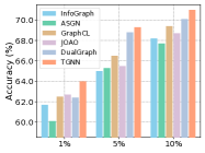
(a) PROTEINS

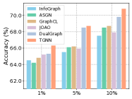
(b) DD

Figure 2: Results of TGNN and baselines with different labeling ratios on two datasets PROTEINS and DD.

Influence of Labeling Ratio. We vary the labeling ratio of training data on PROTEINS and DD in Figure 2. From the results, we can clearly see that the performance of all models generally improves as the number of available labeled data increases, demonstrating that adding more labeled data is an efficient way to boost the performance. Among these methods, TGNN achieves the best results, showing that sufficiently integrating graph topology information from complementary views can indeed benefit the performance.

Methods	PROTEINS	IMDB-B	REDDIT-B
MP-Sup	$63.3\pm 1.4$	$63.4\pm 2.1$	$69.8\pm 1.1$
GK-Sup	$62.6\pm 0.8$	$55.4\pm 1.7$	$65.3\pm 0.6$
MP-Ensemble	$68.1\pm 1.5$	$69.8\pm 1.2$	$73.7\pm 1.1$
GK-Ensemble	$66.9\pm 1.7$	$60.5\pm 1.8$	$70.8\pm 0.8$
TGNN w/o Aug	$69.3\pm 0.8$	$71.7\pm 1.3$	$75.8\pm 0.7$
TGNN (Ours)	71.0 $\pm$ 0.7	72.8 $\pm$ 1.7	76.3 $\pm$ 1.3

Table 3: Ablation study of TGNN with its variants.

4.3 Ablation Study

We investigate a few variants to demonstrate the effect of every part of our model: (1) MP-Sup trains an MPNN (i.e., $f_{\theta}$) solely on labeled in a supervised manner. (2) GK-Sup trains a graph kernel neural network (i.e., $g_{\phi}$) solely on labeled data. (3) MP-Ensemble replaces the graph kernel module with another message passing module with different initialization. (4) GK-Ensemble replaces the message passing module with another graph kernel module with different initialization. (5) TGNN w/o Aug. removes the graph augmentation strategy before feeding graphs into the twin modules.

We present the results of different model variants in Table 3. First, we can clearly observe that on most datasets, MP-Sup outperforms GK-Sup. Maybe the reason is that the message passing module can utilize node attributes while the graph kernel module fails. Second, MP-Ensemble (GK-Ensemble) outperforms MP-Sup (GK-Sup), indicating our consistency learning framework can improve the model through ensemble learning. Third, our full model beats both two ensemble models, indicating the superiority of exploring similarity from complementary views. Finally, with the graph augmentation, our full model achieves better performance, showing that graph augmentation can produce generalized graph representations beneficial to graph classification.

4.4 Hyper-parameter Study

We further examine the hyper-parameter sensitivity of our TGNN w.r.t. different embedding dimensions of hidden layers $d$ and the maximum length of random walk $P$ as shown in Figure 3. We first vary $d$ in $\{8,16,32,64,128\}$ with all other hyper-parameters fixed. It is clear that the performance saturates as the embedding dimensions reach around $64$. This is because a larger dimensionality brings a stronger representation ability at the early stage, but might lead to overfitting as the continuously increasing of $d$. We further vary $P$ in $\{1,2,3,4,5,6\}$ while fixing all other hyper-parameters. We observe that the performance tends to first increase and then decrease. A too-small $P$ would lead to limited topological exploration space while a large $P$ may introduce instability and fail to distinguish graph similarity.

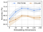
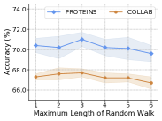
Figure 3: Hyper-parameter sensitivity study of TGNN.

4.5 Case Study

We investigate the power of our graph kernel module to show the superiority of explicitly exploring topology information. First, we show two cases on REDDIT-M-5k in Figure 4, where two unlabeled examples are annotated with both the message passing module and graph kernel module. We can find that both samples are classified into wrong categories by $f_{\theta}$, while $g_{\phi}$ revises the wrong prediction successfully, which demonstrates that our graph kernel module is an important supplement for graph classification. The potential reason is that the graph kernel module is able to capture clearer topology information embedded in graph substructures. Furthermore, we visualize several hidden graphs derived from the graph kernel module on PROTEINS. From Figure 5, we can clearly see that our module is able to generate various kinds of graph substructures, so as to effectively capture the rich topological information in the dataset.

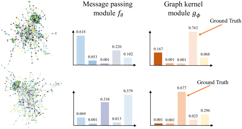
Figure 4: Visualize the power of graph kernel on REDDIT-M-5k.

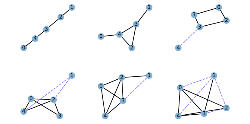
Figure 5: Illustration of hidden graphs extracted from our graph kernel module on PROTEINS.

5 Conclusion

This paper presents a Twin Graph Neural Network (TGNN), a joint optimization framework that combines the advantages of graph neural networks and graph kernels. TGNN consists of twin modules named message passing module and graph kernel module, which explore graph topology information from complementary views. Furthermore, a semi-supervised framework is proposed to encourage the consistency between two similarity distributions in different embedding spaces. Extensive empirical studies show that our approach outperforms competitive baselines by a large margin.

References

- Adhikari et al. [2018] Bijaya Adhikari, Yao Zhang, Naren Ramakrishnan, and B Aditya Prakash. Sub2vec: Feature learning for subgraphs. In PAKDD, 2018.
- Chen et al. [2020] Dexiong Chen, Laurent Jacob, and Julien Mairal. Convolutional kernel networks for graph-structured data. In ICML, 2020.
- Gilmer et al. [2017] Justin Gilmer, Samuel S Schoenholz, Patrick F Riley, Oriol Vinyals, and George E Dahl. Neural message passing for quantum chemistry. In ICML, 2017.
- Grandvalet and Bengio [2005] Yves Grandvalet and Yoshua Bengio. Semi-supervised learning by entropy minimization. In NeurIPS, 2005.
- Hao et al. [2020] Zhongkai Hao, Chengqiang Lu, Zhenya Huang, Hao Wang, Zheyuan Hu, Qi Liu, Enhong Chen, and Cheekong Lee. Asgn: An active semi-supervised graph neural network for molecular property prediction. In KDD, 2020.
- Hinton et al. [2014] Geoffrey Hinton, Oriol Vinyals, and Jeff Dean. Distilling the knowledge in a neural network. In NeurIPS Workshop, 2014.
- Ju et al. [2022] Wei Ju, Xiao Luo, Zeyu Ma, Junwei Yang, Minghua Deng, and Ming Zhang. Ghnn: Graph harmonic neural networks for semi-supervised graph-level classification. Neural Networks, 2022.
- Kashima et al. [2003] Hisashi Kashima, Koji Tsuda, and Akihiro Inokuchi. Marginalized kernels between labeled graphs. In ICML, 2003.
- Kipf and Welling [2017] Thomas N Kipf and Max Welling. Semi-supervised classification with graph convolutional networks. In ICLR. 2017.
- Kojima et al. [2020] Ryosuke Kojima, Shoichi Ishida, Masateru Ohta, Hiroaki Iwata, Teruki Honma, and Yasushi Okuno. kgcn: a graph-based deep learning framework for chemical structures. Journal of Cheminformatics, 2020.
- Laine and Aila [2017] Samuli Laine and Timo Aila. Temporal ensembling for semi-supervised learning. In ICLR, 2017.
- Lee and others [2013] Dong-Hyun Lee et al. Pseudo-label: The simple and efficient semi-supervised learning method for deep neural networks. In ICML Workshop, 2013.
- Li et al. [2019] Jia Li, Yu Rong, Hong Cheng, Helen Meng, Wenbing Huang, and Junzhou Huang. Semi-supervised graph classification: A hierarchical graph perspective. In WWW, 2019.
- Long et al. [2021] Qingqing Long, Yilun Jin, Yi Wu, and Guojie Song. Theoretically improving graph neural networks via anonymous walk graph kernels. In WWW, 2021.
- Lu et al. [2019] Chengqiang Lu, Qi Liu, Chao Wang, Zhenya Huang, Peize Lin, and Lixin He. Molecular property prediction: A multilevel quantum interactions modeling perspective. In AAAI, 2019.
- Luo et al. [2022] Xiao Luo, Wei Ju, Meng Qu, Chong Chen, Minghua Deng, Xian-Sheng Hua, and Ming Zhang. Dualgraph: Improving semi-supervised graph classification via dual contrastive learning. In ICDE, 2022.
- Miyato et al. [2018] Takeru Miyato, Shin-ichi Maeda, Masanori Koyama, and Shin Ishii. Virtual adversarial training: a regularization method for supervised and semi-supervised learning. IEEE TPAMI, 2018.
- Narayanan et al. [2017] Annamalai Narayanan, Mahinthan Chandramohan, Rajasekar Venkatesan, Lihui Chen, Yang Liu, and Shantanu Jaiswal. graph2vec: Learning distributed representations of graphs. arXiv preprint arXiv:1707.05005, 2017.
- Nikolentzos and Vazirgiannis [2020] Giannis Nikolentzos and Michalis Vazirgiannis. Random walk graph neural networks. In NeurIPS, 2020.
- Shervashidze et al. [2011] Nino Shervashidze, Pascal Schweitzer, Erik Jan Van Leeuwen, Kurt Mehlhorn, and Karsten M Borgwardt. Weisfeiler-lehman graph kernels. JMLR, 2011.
- Spielman [2007] Daniel A Spielman. Spectral graph theory and its applications. In FOCS, 2007.
- Sun et al. [2020] Fan-Yun Sun, Jordan Hoffmann, Vikas Verma, and Jian Tang. Infograph: Unsupervised and semi-supervised graph-level representation learning via mutual information maximization. In ICLR, 2020.
- Tarvainen and Valpola [2017] Antti Tarvainen and Harri Valpola. Mean teachers are better role models: Weight-averaged consistency targets improve semi-supervised deep learning results. In NeurIPS, 2017.
- Veličković et al. [2017] Petar Veličković, Guillem Cucurull, Arantxa Casanova, Adriana Romero, Pietro Lio, and Yoshua Bengio. Graph attention networks. In ICLR. 2017.
- Vishwanathan et al. [2010] S Vichy N Vishwanathan, Nicol N Schraudolph, Risi Kondor, and Karsten M Borgwardt. Graph kernels. JMLR, 2010.
- Xu et al. [2019] Keyulu Xu, Weihua Hu, Jure Leskovec, and Stefanie Jegelka. How powerful are graph neural networks? In ICLR, 2019.
- Yanardag and Vishwanathan [2015] Pinar Yanardag and SVN Vishwanathan. Deep graph kernels. In KDD, 2015.
- Ying et al. [2018] Zhitao Ying, Jiaxuan You, Christopher Morris, Xiang Ren, Will Hamilton, and Jure Leskovec. Hierarchical graph representation learning with differentiable pooling. In NeurIPS, 2018.
- You et al. [2020] Yuning You, Tianlong Chen, Yongduo Sui, Ting Chen, Zhangyang Wang, and Yang Shen. Graph contrastive learning with augmentations. In NeurIPS, 2020.
- You et al. [2021] Yuning You, Tianlong Chen, Yang Shen, and Zhangyang Wang. Graph contrastive learning automated. In ICML, 2021.