Theoretical and numerical comparison of quantum- and classical embedding models for optical spectra

Abstract

Quantum-mechanical (QM) and classical embedding models approximate a supermolecular quantum-chemical calculation. This is particularly useful when the supermolecular calculation has a size that is out of reach for present QM models. Although QM and classical embedding methods share the same goal, they approach this goal from different starting points. In this study, we compare the polarizable embedding (PE) and frozen-density embedding (FDE) models. The former is a classical embedding model, whereas the latter is a density-based QM embedding model.

Our comparison focuses on solvent effects on optical spectra of solutes. This is a typical scenario where super-system calculations including the solvent environment become prohibitively large. We formulate a common theoretical framework for PE and FDE models and systematically investigate how PE and FDE approximate solvent effects. Generally, differences are found to be small, except in cases where electron spill-out becomes problematic in the classical frameworks. In these cases, however, atomic pseudopotentials can reduce the electron-spill-out issue.

1 Introduction

Quantum-mechanical (QM) methods are indispensable for the calculation of optical spectra, but their use often becomes computationally too demanding for large systems. Embedding schemes have been introduced to circumvent the full, super-system QM calculation by including large environments through an effective embedding operator.
The definition of an embedding model requires that the system is split into an active system and the remaining part (”the environment”).[1, 2, 3, 4] Embedding approaches can be divided into two main classes: (i) QM-classical embedding approaches describe the active system by a QM method, whereas all interactions between the active system and environment (as well as the environment itself) are treated by a classical description. (ii) QM-QM embedding describes both active system and environment with QM methods (either on the same or different footings). In this case, the interaction between active system and the environment also contains QM contributions.
For optical properties, the electrostatic interaction between the active system and the environment is often the dominating embedding contribution. In traditional QM-classical approaches, this contribution is modeled through (atomic) point charges in the environment.[4] The point-charge model is, however, insufficient in many cases.[1, 5, 6, 7, 8, 9] Therefore, a large number of more advanced embedding schemes have been developed over the years.[10, 11, 12, 7, 13, 14, 15, 16, 17, 18, 19, 20, 5, 21, 22, 23]
In this work, we employ an advanced QM-classical embedding model, namely the polarizable embedding (PE) model[20]. In this model, point charges in the environment are replaced by a multipole expansion. Additionally, PE incorporates the environment polarization through anisotropic electronic dipole–dipole polarizabilities. The parameters for the environment (i.e. multipoles and polarizabilities) are obtained from QM calculations on isolated fragments. If the environment is a solvent, these fragments are most naturally defined as solvent molecules.
In the class of QM-QM embedding methods, the total system is expressed by means of fragments or subsystems [24, 25, 26, 27]: Within density functional theory (DFT) this is known as subsystem DFT.[28] All subsystems are described by their electron densities, which are obtained by quantum-chemical calculations. The interaction of the environment subsystems with the active subsystem is then recovered through an embedding potential, which contains quantum-mechanical contributions. This potential is dependent on all other subsystem’s electron densities.[29, 28] In practice, the environmental electron densities are commonly kept frozen, so that only the active subsystem’s electron density is polarized. In this frozen-density embedding (FDE) approach[29], the effect of the environment’s polarizability can be incorporated by self-consistently cycling through all subsystems in a so-called freeze-and-thaw scheme.[25, 27, 29, 30, 28]
Both embedding classes share, hence, a common goal and have been employed to show that polarization effects originating from the environment can play a significant role in the accurate calculation of local optical properties.[31, 8, 32, 33, 34] Yet, direct numerical comparisons have been rare due to their different formulations and implementations.[35, 36] We recently developed a common theoretical framework[17] encompassing both fragmentation-based QM-QM and QM-classical embedding methods with a special focus on FDE and PE. This framework was employed to dissect how the two classes of embedding models describe the interactions between the active system and the environment. We here continue this comparison by quantifying how the theoretical differences manifest numerically for optical properties of two solvated systems, employing a supermolecular calculation as a reference.

a) [atom sep=2em][:90]*6(=(-NO_2)-=-(-NH_2)=-)

b)

[atom sep=2em]⊖OOC-[:-18]*5(=-=(-(*5(-S-(-(*5(=-=(-(*5(-S-(-(*5(=-=(-COO⊖)-S-)))=-(-[:120]-[:60]COO⊖)=)))-S-)))=(-[:60]-[:120]⊖OOC)-=)))-S-)

Figure 1: Dyes considered in this work: (a) para-nitroaniline (b) pentameric formyl thiophene acetic acid

Our target systems (fig. 1) are two fluorescent dyes whose excited-state properties are known to be sensitive to solvent effects: The first target system is para-nitroaniline (pNA), which has been studied with several different embedding schemes [37, 38, 39, 40, 7, 8]. Yet, the performance of the QM-QM and QM-classical embedding schemes have never been compared in a combined study. The second test case is pentameric formyl thiophene acetic acid (pFTAA), a luminescent biomarker developed for fluorescence imaging for amyloid proteins.[41] The mechanism occurring with the chromophore embedded in the protein site is not fully understood yet, but it is known that its properties strongly depend on the solvent–solute interactions and the conformation of the molecule.[42, 43, 44, 45] Notably, pFTAA is an anionic system and therefore poses somewhat different challenges in the description of the solute–solvent interaction than pNA.

This paper is organized as follows. We first briefly introduce the PE and FDE scheme in the common theoretical framework as derived in previous work[17] (sec. 2). In particular, we point out similarities and differences between these schemes. We describe the computational setup, that was developed to enable us to compare the embedding methods on equal footing (sec. 2.1). In section 3, the computational details are given. Subsequently, the results are presented and discussed (sec. 4). Finally, in the last section (sec. 5), we conclude and summarize the study.

2 Theoretical Background

In this section, we give a brief overview of the density-based QM-QM embedding and classical PE methods. For a more detailed derivation, reviews, and further extensions of the presented models we refer to Refs. [17, 14, 15, 16, 46, 28, 47, 48, 36]. Here, we use the common framework developed in Ref. [17].

Embedding schemes commonly focus on a selected, active subsystem A. The remaining parts are labelled the environment (env). The total energy can be written as the sum of the energy functionals of the respective electron densities $\rho_{\mathrm{A}}$ and $\rho_{\mathrm{env}}$,

$$E_{\mathrm{tot}}[\rho_{\mathrm{tot}}]=E_{\mathrm{A}}[\rho_{\mathrm{A}}]+E_{\mathrm{env}}[\rho_{\mathrm{env}}]+E_{\text{int}}[\rho_{\mathrm{A}},\rho_{\mathrm{env}}],$$ (1)

where $E_{\mathrm{tot}}[\rho_{\mathrm{tot}}]$ and $E_{\mathrm{A}}[\rho_{\mathrm{A}}]$ denote the total energy functional and the energy functional of the active subsystem A, respectively. The $E_{\text{int}}[\rho_{\mathrm{A}},\rho_{\mathrm{env}}]$ term defines the interaction energy, i.e. $E_{\mathrm{int}}[\rho_{\mathrm{A}},\rho_{\mathrm{env}}]=E_{\mathrm{tot}}[\rho_{\text{tot}}]-E_{\mathrm{A}}[\rho_{\mathrm{A}}]-E_{\mathrm{env}}[\rho_{\mathrm{env}}]$, where we assume $\rho_{\text{tot}}=\rho_{\mathrm{A}}+\rho_{\mathrm{env}}$. The environment density can analogously be approximated as a sum of all environmental (subsystem) densities, $\rho_{X}$, by $\rho_{\mathrm{env}}=\sum_{X\neq\mathrm{A}}\rho_{X}$. We further decompose the interaction energy into Coulomb (classical), $E_{\text{int}}^{\text{C}}[\rho_{\mathrm{A}},\rho_{\mathrm{env}}]$, and QM contributions, $E_{\text{int}}^{\text{QM}}[\rho_{\mathrm{A}},\rho_{\mathrm{env}}]$,

$$E_{\text{int}}[\rho_{\mathrm{A}},\rho_{\mathrm{env}}]=E_{\text{int}}^{\text{C}}[\rho_{\mathrm{A}},\rho_{\mathrm{env}}]+E_{\text{int}}^{\text{QM}}[\rho_{\mathrm{A}},\rho_{\mathrm{env}}],$$ (2)

where both contributions can be obtained analogously to eq. (1).

The Coulomb part is included in both density-based and classical embedding schemes. In the density-based QM-QM embedding schemes this part is expressed as

$$E_{\mathrm{int}}^{\mathrm{C}}[\rho_{\mathrm{A}},\rho_{\mathrm{env}}]= \sum_{X\neq\mathrm{A}}\int\int\frac{\rho_{\mathrm{A}}(\mathbf{r}_{\text{a}})\rho_{X}(\mathbf{r}_{x})}{|\mathbf{r}_{\text{a}}-\mathbf{r}_{x}|}{\mathrm{d}}\mathbf{r}_{\text{a}}{\mathrm{d}}\mathbf{r}_{x}-\sum_{X\neq\mathrm{A}}\sum_{I\in\mathrm{A}}\int\frac{Z_{I}\rho_{X}(\mathbf{r}_{x})}{|\mathbf{R}_{I}-\mathbf{r}_{x}|}{\mathrm{d}}\mathbf{r}_{x}$$

$$-\sum_{X\neq\mathrm{A}}\sum_{J\in X}\int\frac{Z_{J}\rho_{\mathrm{A}}(\mathbf{r}_{\text{a}})}{|\mathbf{R}_{J}-\mathbf{r}_{\text{a}}|}{\mathrm{d}}\mathbf{r}_{\text{a}}+\sum_{X\neq\mathrm{A}}\sum_{I\in\mathrm{A}}\sum_{J\in X}\frac{Z_{I}Z_{J}}{|\mathbf{R}_{I}-\mathbf{R}_{J}|},$$ (3)

where $\mathbf{R}_{I/J}$ denote nuclear coordinates, $\mathbf{r}_{a/x}$ denote electronic coordinates, and $Z_{I/J}$ are nuclear charges. The interaction of the environment with the active subsystem is included via Coulomb [and possibly quantum-mechanical (QM)] contributions through an effective embedding operator. The effective Hamiltonian for subsystem A can be expressed as

$$\hat{H}_{\mathrm{A}}^{\text{eff}}=\hat{H}_{\mathrm{A}}+\hat{v}_{\text{A}}^{\mathrm{emb}}=\hat{H}_{\mathrm{A}}+\int\hat{\rho}_{\mathrm{A}}(\mathbf{r}_{\mathrm{a}}){v}_{\text{A}}^{\mathrm{emb}}(\mathbf{r}_{\mathrm{a}})\mathrm{d}\mathbf{r}_{\mathrm{a}},$$ (4)

where the density operator $\hat{\rho}_{\mathrm{A}}(\mathbf{r}_{\text{a}})=\sum_{i\in\mathrm{A}}\delta(\mathbf{r}_{i}-\mathbf{r}_{\text{a}})$ defines the connection between the Hamiltonian with electron-based coordinates and density-based expressions with real-space coordinates. We define the embedding operator via a real-space potential,

$$v_{\mathrm{A}}^{\text{emb}}(\mathbf{r}_{\mathrm{a}})= \frac{\delta}{\delta\rho_{\mathrm{A}}}(E_{\mathrm{tot}}[\rho_{\mathrm{tot}}]-E_{\mathrm{A}}[\rho_{\mathrm{A}}])$$

$$= \frac{\delta E_{\mathrm{tot}}^{\mathrm{C}}[\rho_{\mathrm{tot}}]}{\delta\rho_{\mathrm{A}}}-\frac{\delta E^{\mathrm{C}}_{\mathrm{A}}[\rho_{\mathrm{A}}]}{\delta\rho_{\mathrm{A}}}+\frac{\delta E_{\mathrm{tot}}^{\mathrm{QM}}[\rho_{\mathrm{tot}}]}{\delta\rho_{\mathrm{A}}}-\frac{\delta E^{\mathrm{QM}}_{\mathrm{A}}[\rho_{\mathrm{A}}]}{\delta\rho_{\mathrm{A}}}.$$ (5)

In FDE, the environmental density $\rho_{\text{env}}$ is kept frozen so that the total embedding potential resulting from eq. (5) becomes

$$v_{\mathrm{A}}^{\mathrm{FDE}}(\mathbf{r}_{a})= v_{\mathrm{A}}^{\mathrm{C(FDE)}}[\rho_{\mathrm{env}}](\mathbf{r}_{\mathrm{a}})+v_{\text{A}}^{\text{nadd,kin}}[\rho_{\mathrm{A}},\rho_{\mathrm{env}}](\mathbf{r}_{\mathrm{a}})+v_{\text{A}}^{\text{nadd,xc}}[\rho_{\mathrm{A}},\rho_{\mathrm{env}}](\mathbf{r}_{\mathrm{a}}),$$ (6)

with the Coulomb potential only depending on $\rho_{A}$ and the (frozen) densities of the environment

$$v_{\mathrm{A}}^{\mathrm{C(FDE)}}[\rho_{\mathrm{env}}](\mathbf{r}_{\mathrm{a}}) =\frac{\delta E_{\mathrm{int}}^{\mathrm{C}}[\rho_{\mathrm{A}},\rho_{\mathrm{env}}]}{\delta\rho_{\mathrm{A}}}$$

$$=-\sum_{X\neq\mathrm{A}}\sum_{J\in X}\frac{Z_{J}}{|\mathbf{r}_{\mathrm{a}}-\mathbf{R}_{J}|}+\sum_{X\neq\mathrm{A}}\int\frac{\rho_{X}(\mathbf{r}_{x})}{|\mathbf{r}_{\mathrm{a}}-\mathbf{r}_{x}|}{\mathrm{d}}\mathbf{r}_{x},$$ (7)

where $E_{\mathrm{int}}^{\mathrm{C}}[\rho_{\mathrm{A}},\rho_{\mathrm{env}}]$ is defined in eq. (3). The QM contributions from eq. (5) are comprised of kinetic and an exchange–correlation (xc) parts, represented by $v_{\text{A}}^{\text{nadd,kin}}$ and $v_{\text{A}}^{\text{nadd,xc}}$ in eq. (6). In practical calculations, these contributions are often approximated by orbital-free DFT methodologies[29, 28, 47], though for $v_{\text{A}}^{\text{nadd,kin}}$ also orbital-dependent projection schemes have been reported.[49, 50, 51, 52, 53, 54, 55, 56, 57, 58, 59, 60, 61]
The application of a fixed $\rho_{\mathrm{env}}$ in FDE leads to several possible choices of frozen densities. The crudest approximation is to use the density from the isolated fragments by a superscript $\{\rho^{(0)}_{X}\}$ (and likewise we also can define $\rho^{(0)}_{A}$). Allowing the active subsystem A to relax by submitting $\rho_{\mathrm{A}}$ to a self-consistent-field optimization in the frozen environment density, $\rho_{\mathrm{env}}^{(0)}$, leads to a relaxed density $\rho_{A}^{\mathrm{(1)}}$. In terms of density-based embedding schemes, this approach directly refers to FDE.[29] It yields a relaxed energy for the active subsystem $E_{\mathrm{A}}[\rho_{\mathrm{A}}^{(1)}]$.

The relaxation of $\rho_{A}^{(0)}$ to $\rho_{A}^{(1)}$ can be done for all fragments in a step-wise manner until self-consistency to obtain the relaxed densities $\rho_{A}^{(2)}$ and $\rho_{\mathrm{env}}^{(2)}$. This is denoted a freeze-and-thaw procedure[62]. Formally, the mutual polarization of the densities in the ground state of the super system is recovered when performing a sufficient number of freeze-and-thaw cycles.

In contrast to that, the PE methods approximate both static electrostatics and polarization solely based on frozen densities in the environment, $\rho_{\text{env}}^{(0)}=\sum_{X\neq A}\rho^{(0)}_{X}$. An expression for the total energy comparable to eq. (1) can then be obtained through Rayleigh–Schrödinger perturbation theory,

$$E_{\mathrm{tot}}\approx E^{(0)}+E^{(1)}+E^{(2)}.$$ (8)

By expressing the interaction between the subsystems as perturbations of the energy, the zeroth-order perturbation can be identified as the isolated subsystem energies. Thus, from eq. (1) we identify $E^{(0)}=E_{\mathrm{A}}[\rho_{\mathrm{A}}^{(0)}]+E_{\mathrm{env}}[\rho_{\mathrm{env}}^{(0)}]$ and the interaction energy ($E_{\mathrm{int}}[\rho_{\mathrm{A}}^{(0)},\rho_{\mathrm{env}}^{(0)}]$) must therefore come through the higher-order energy corrections. Indeed, the first-order correction corresponds to eq. (3) with frozen densities, i.e., $E^{\mathrm{C}}_{\mathrm{int}}[\rho^{(0)}_{\mathrm{A}},\rho^{(0)}_{\mathrm{env}}]$. The PE model further approximates $E^{\mathrm{C}}_{\mathrm{int}}[\rho^{(0)}_{\mathrm{A}},\rho^{(0)}_{\mathrm{env}}]$ through a multipole expansion[63, 64, 65], i.e.,

$$E^{(1)}=E^{\mathrm{C}}_{\mathrm{int}}[\rho^{(0)}_{\mathrm{A}},\rho^{(0)}_{\mathrm{env}}]\approx E^{\mathrm{mult}}_{\mathrm{int}}[\rho^{(0)}_{\mathrm{A}},\rho^{(0)}_{\mathrm{env}}].$$ (9)

The multipole expansion employs individual atoms of the subsystems/fragments as expansion points ($\{\mathbf{R}_{s}\}$ or in short sites, $s$). The multipole expansion can thus be written as

$$E^{\mathrm{mult}}_{\mathrm{int}}[\rho^{(0)}_{\mathrm{A}},\{\rho^{(0)}_{X}\}]= \sum_{X\neq A}\sum_{s\in X}\left(-\int\rho^{(0)}_{\mathrm{A}}(\mathbf{r}_{\text{a}})T^{(0)}_{s\mathrm{a}}\text{d}\mathbf{r}_{\text{a}}+\sum_{I\in A}Z_{I}T^{(0)}_{sI}\right)q_{\mathrm{s}}[\rho_{\mathrm{X}}^{(0)}]$$

$$-\sum_{X\neq A}\sum_{s\in X}\left(-\int\rho^{(0)}_{\mathrm{A}}(\mathbf{r}_{\text{a}})\mathbf{T}^{(1)}_{s\mathrm{a}}\text{d}\mathbf{r}_{\text{a}}+\sum_{I\in A}Z_{I}\mathbf{T}^{(1)}_{sI}\right)\bm{\mu}_{s}[\rho_{X}^{(0)}]+\cdots.$$ (10)

In the above equation, we have defined the interaction operators $\mathbf{T}^{(k)}_{s\mathrm{a}}=\frac{\partial^{k_{x}+k_{y}+k_{z}}}{\partial x^{k_{x}}_{a}\partial y^{k_{y}}_{a}\partial z^{k_{z}}_{a}}|\mathbf{R}_{\mathrm{a}}-\mathbf{R}_{s}|^{-1}$ that describe interactions at point $a$ due to site $s$. Moreover, the multipole moment operator of $k$’th order at site $s$ is defined as $\mathbf{Q}_{s}^{(k)}[\rho^{(0)}_{X}]=\langle\Psi^{(0)}_{X}|\hat{\mathbf{Q}}^{(k)}_{\mathrm{s}}|\Psi^{(0)}_{X}\rangle$. The term for zeroth-order moments represents the charge contribution $\hat{\mathbf{Q}}^{(0)}_{\mathrm{s}}=\hat{\mathbf{q}}_{\mathrm{s}}$, the first-order term denotes the dipole contribution $\hat{\mathbf{Q}}^{(1)}_{\mathrm{s}}=\hat{\boldsymbol{\mu}}_{\mathrm{s}}$ and so on. In the following, we combine the two sums over fragments $X$ and sites $s$ into one sum over all sites $s$.

The mutual polarization effects are approximately covered by the second-order correction[64]

$$E^{(2)} =E_{\text{A}}^{\text{pol}}+E_{\text{env}}^{\text{pol}}+E^{\text{disp}}.$$ (11)

We focus on the following only on the polarization part, while neglecting $E^{\mathrm{disp}}$. The environment polarization energy, $E_{\mathrm{env}}^{\mathrm{pol}}$, can be described as

$$E_{\mathrm{env}}^{\mathrm{pol}}[\rho^{(0)}_{\mathrm{A}}]=-\frac{1}{2}\boldsymbol{\mathcal{E}}^{T}[\rho^{(0)}_{\mathrm{A}}]\cdot\boldsymbol{\mathcal{\mu}}^{\mathrm{ind}}[\rho^{(0)}_{\mathrm{A}}],$$ (12)

and $E_{\text{A}}^{\text{pol}}$ can in principle be obtained analogously. This part is, however, inherently included in the QM model for the active system. The field $\boldsymbol{\mathcal{E}}$ is defined as the sum of the fields from electrons in system A, nuclei in system A, and the multipoles in the environment

$$\boldsymbol{\mathcal{E}}[\rho^{(0)}_{\mathrm{A}}]=\boldsymbol{\mathcal{E}}^{\mathrm{e}}_{\mathrm{A}}[\rho^{(0)}_{\mathrm{A}}]+\boldsymbol{\mathcal{E}}^{\mathrm{n}}_{\mathrm{A}}+\boldsymbol{\mathcal{E}}^{\mathrm{mult}}_{\mathrm{env}}.$$ (13)

The induced dipole moment on site $s$ can then be obtained as

$$\boldsymbol{\mu}^{\mathrm{ind}}_{s}[\rho^{(0)}_{\mathrm{A}}]=\bm{\alpha}_{s}\cdot\left(\boldsymbol{\mathcal{E}}_{s}[\rho^{(0)}_{\mathrm{A}}]+\sum_{s^{\prime}\neq s}\mathbf{T}^{(2)}_{ss^{\prime}}\boldsymbol{\mu}^{\mathrm{ind}}_{s^{\prime}}\right),$$ (14)

where $\bm{\alpha}_{s}$ is the (static) point-polarizability localized in site $s$ and $\boldsymbol{\mathcal{E}}_{s}[\rho^{(0)}_{\mathrm{A}}]$ the field in eq. (13) on site $s$. Note that the induced dipole on site $s$ depends on the field generated from the induced dipoles on all remaining sites. Thus, a self-consistent optimization is required to obtain the induced dipole moment $\boldsymbol{\mu}^{\mathrm{ind}}_{s}$. This optimization problem can be written as

$$\boldsymbol{\mu}^{\mathrm{ind}}_{s}[\rho_{\mathrm{A}}^{(0)}]=\sum_{t}\mathbf{R}_{ts}\boldsymbol{\mathcal{E}}_{\mathrm{A},s}[\rho^{(0)}_{\mathrm{A}}],$$ (15)

where the so-called classical response matrix, $\mathbf{R}$, is given as

$$\mathbf{R}=\begin{pmatrix}\boldsymbol{\alpha}_{1}^{-1}&-\mathbf{T}_{12}^{(2)}&\dots&-\mathbf{T}_{1S}^{(2)}\\ -\mathbf{T}_{21}^{(2)}&\boldsymbol{\alpha}_{2}^{-1}&\dots&-\mathbf{T}_{2S}^{(2)}\\ \vdots&\vdots&\ddots&\vdots\\ -\mathbf{T}_{S1}^{(2)}&-\mathbf{T}_{S2}^{(2)}&\dots&\boldsymbol{\alpha}_{S}^{-1}\\ \end{pmatrix}^{-1}.$$ (16)

The total energy (in eq. 1) is now defined by combining eqs. (8)–(11),

$$E^{\mathrm{PE}}_{\mathrm{tot}}[\rho_{\mathrm{A}},\rho_{\mathrm{env}}^{(0)}]=E_{\mathrm{A}}^{\mathrm{PE}}[\rho_{\mathrm{A}},\rho_{\mathrm{env}}^{(0)}]+E_{\mathrm{env}}^{\mathrm{PE}}[\rho_{\mathrm{env}}^{(0)},\rho_{\mathrm{A}}]+E^{\mathrm{mult}}_{\mathrm{int}}[\rho_{\mathrm{A}},\rho^{(0)}_{\mathrm{env}}],$$ (17)

where we skip the superscript for $\rho_{\mathrm{A}}$ to denote that it is subject to change in the self-consistent-field (SCF) procedure performed during the optimization of the QM system (note that eq. (15) will then have to be solved within each SCF cycle). The environment density $\rho_{\mathrm{env}}^{(0)}$ remains the isolated density of the environment fragments (represented by a multipole expansion). For consistency with the definition in eq. (1), we have written the total energy in eq. (17) as a sum of the energies of the active system A and the environment plus an interaction energy, where we have combined the energy of the isolated subsystem and polarization in the term $E^{\mathrm{PE}}_{\mathrm{A}}[\rho_{\mathrm{A}},\rho_{\mathrm{env}}^{(0)}]=E_{\mathrm{A}}[\rho_{\mathrm{A}}]+E_{\mathrm{A}}^{\mathrm{pol}}[\rho^{(0)}_{\mathrm{env}}]$. The term $E^{\mathrm{PE}}_{\mathrm{env}}[\rho_{\mathrm{env}}^{(0)},\rho_{\mathrm{A}}]$ is defined in a similar fashion.

With this starting point, a PE embedding potential according to eq. (5) is derived in Ref. [17]. The emanating formalism can be summarized as follows

$$v_{\text{A}}^{\mathrm{PE}}= \frac{\delta E_{\mathrm{tot}}^{\mathrm{PE}}[\rho_{\mathrm{A}},\rho_{\text{env}}^{(0)}]}{\delta\rho_{\mathrm{A}}}-\frac{\delta E_{\mathrm{A}}^{\mathrm{PE}}[\rho_{\mathrm{A}}]}{\delta\rho_{\mathrm{A}}}={v}^{\mathrm{mult}}+{v}^{\mathrm{pol}},$$ (18)

where the two operators are defined as

$${v}^{\mathrm{mult}} =\sum_{s}\sum_{k=0}\frac{(-1)^{|k|}}{k!}{\mathbf{T}}^{(k)}_{s\mathrm{a}}(\mathbf{r}_{\mathrm{a}})\mathbf{Q}^{(k)}_{s}$$ (19)

and

$${v}^{\mathrm{pol}} =\sum_{s}\Big{(}\boldsymbol{\mu}^{\mathrm{ind}}_{s}[\rho_{\mathrm{A}}]\Bigr{)}^{T}\ \boldsymbol{\varepsilon}^{\mathrm{e}}_{\mathrm{A},s}(\mathbf{r}_{\mathrm{a}}),$$ (20)

The field potential $\boldsymbol{\varepsilon}^{\mathrm{e}}_{\mathrm{A},s}(\mathbf{r}_{\mathrm{a}})$ is the component of the electronic part of the electric field operator at the site $s$, defined in real-space coordinates as,

$$\boldsymbol{\varepsilon}^{\mathrm{e}}_{\mathrm{A},s}(\mathbf{r}_{\mathrm{a}})=\frac{\delta\mathcal{E}^{\mathrm{e}}_{\mathrm{A},s}[\rho_{\mathrm{A}}(\mathbf{r}_{\mathrm{a}})]}{\delta\rho_{\mathrm{A}}(\mathbf{r}_{\mathrm{a}})}.$$ (21)

where $\mathcal{E}^{\mathrm{e}}_{\mathrm{A},s}[\rho_{\mathrm{A}}(\mathbf{r}_{\mathrm{a}})]$ is the electronic component of the field in system A at site $s$ (cf. eq. 13). Thus, ${v}^{\mathrm{mult}}$ corresponds to a multipole approximation of eq. (7), where only $\rho^{(0)}_{X}$ are employed. Similarly, ${v}^{\mathrm{pol}}$ approximates the effect of mutual polarization, i.e., moving from $\rho^{(0)}_{X}$ to $\rho^{(2)}_{X}$ in eq. (7). The QM contributions from eq. (6) are not included in standard PE.

Optical spectra are in this work obtained by linear response theory. To incorporate embedding contributions of the introduced models in local response calculations, we employ the commonly used framework of time-dependent DFT (TD-DFT). Therefore, we add the embedding potential $v_{\text{emb}}$ to the Kohn-Sham operator of the vacuum system $\hat{f}_{\text{iso}}$

$$\hat{f}_{\text{tot}}=\hat{f}_{\text{iso}}+v_{\text{emb}},$$ (22)

with $v_{\text{emb}}$ being eqs. (6) or (18) for FDE or PE, respectively. Replacing $\hat{f}_{\text{iso}}$ with $\hat{f}_{\text{tot}}$ in the derivation of the response equations leads to a set of modified response equations, that are,

$$\left[\begin{pmatrix}\phantom{-}\mathbf{A}&\mathbf{B}\\ -\mathbf{B}^{*}&-\mathbf{A}^{*}\\ \end{pmatrix}-\omega\begin{pmatrix}~{}\mathbf{1}&\mathbf{0}~{}\\ ~{}\mathbf{0}&\mathbf{1}~{}\\ \end{pmatrix}\right]\begin{pmatrix}\mathbf{X}\\ \mathbf{Y}\end{pmatrix}=0,$$ (23)

with the excitation energies $\omega$ and

$$A_{ai,bj}= \delta_{ij}\delta_{ab}\left(\varepsilon_{a}-\varepsilon_{i}\right)+B_{ai,jb}$$ (24)

$$B_{ai,bj}= \frac{\partial F^{\text{iso}}_{ai}}{\partial P_{bj}}+\frac{\partial\left\langle\phi_{a}|{v}^{\text{emb}}|\phi_{i}\right\rangle}{\partial P_{bj}}.$$ (25)

$F^{\text{iso}}_{ai}$ denotes a Fock matrix element of the isolated system and $P_{bj}$ is an element of the density matrix. The quantities $\varepsilon_{a}$ and $\varepsilon_{i}$ are orbital energies, where occupied orbitals are labelled with $i$ or $j$ and the virtual ones with $a$ or $b$. The orbital energies are eigenvalues of the total Fock operator $\hat{f}_{\text{tot}}$ in eq. (22). Thus, part of the environmental contribution enters through these energies.

For FDE, ${v}^{\text{emb}}$ can be chosen to rely only on $\{\rho^{(0)}_{X}\}$ densities, which we will denote FDE NOPOL. An equivalent contribution can be defined for PE (which we denote PE NOPOL) if only $v^{\mathrm{mult}}$ of eq. (18) is included in $v_{\mathrm{emb}}$. Employing the relaxed densities $\{\rho^{(2)}_{X}\}$ in eq. (5) corresponds to including the ground-state polarization and we denote this model FDE GSPOL. The corresponding model in the PE framework (denoted PE GSPOL) corresponds to employing both $v^{\mathrm{mult}}$ and $v^{\mathrm{pol}}$ of eq. (18) in $v_{\mathrm{emb}}$, while neglecting the $v_{\mathrm{emb}}$ part of $B_{ai,bj}$ in eqs. (24) and (25).

The second term of B requires more attention since the physical content between PE and FDE models is rather different [17]. The term can be identified as

$$\frac{\partial\left\langle\phi_{a}|{v}^{\text{emb}}|\phi_{i}\right\rangle}{\partial P_{bj}}=\left\langle\phi_{a}(\mathbf{r}_{\mathrm{a}})\phi_{b}(\mathbf{r}^{\prime}_{\mathrm{a}})\left|\frac{\delta v^{\mathrm{emb}}_{\mathrm{A}}(\mathbf{r}_{\mathrm{a}})}{\delta\rho_{\mathrm{A}}(\mathbf{r}^{\prime}_{\mathrm{a}})}\right|\phi_{i}(\mathbf{r}_{\mathrm{a}})\phi_{j}(\mathbf{r}^{\prime}_{\mathrm{a}})\right\rangle.$$ (26)

The functional derivative ($\frac{\delta v^{\mathrm{emb}}_{\mathrm{A}}(\mathbf{r}_{\mathrm{a}})}{\delta\rho_{\mathrm{A}}(\mathbf{r}^{\prime}_{\mathrm{a}})}$) for the corresponding embedding scheme can be derived from eqs. (6) and (18) for FDE and PE, respectively.
In the case of FDE, we have a static (ground-state) potential and the Coulomb terms vanish. Thus, only quantum-mechanical terms contribute [66], so that

$$\frac{\delta v^{\mathrm{FDE}}_{\mathrm{A}}(\mathbf{r}_{\mathrm{a}})}{\delta\rho_{\mathrm{A}}(\mathbf{r}^{\prime}_{\mathrm{a}})}= \frac{\delta^{2}E^{\mathrm{QM}}[\rho_{\mathrm{tot}}]}{\delta\rho_{\mathrm{tot}}(\mathbf{r}_{\mathrm{a}})\delta\rho_{\mathrm{tot}}(\mathbf{r}^{\prime}_{\mathrm{a}})}-\frac{\delta^{2}E^{\mathrm{QM}}[\rho_{\mathrm{A}}]}{\delta\rho_{\mathrm{A}}(\mathbf{r}_{\mathrm{a}})\delta\rho_{\mathrm{A}}(\mathbf{r}^{\prime}_{\mathrm{a}})}.$$ (27)

The remaining QM embedding contributions to the response kernel, however, are often small, so that the major environmental effect in the electronic transitions and oscillator strengths are results of differences in the canonical orbitals and orbital energies.[35, 67] The QM contributions to the embedding in the response kernel are, hence, not included in the numerical examples of the present work.

For PE, the functional derivative is obtained from eq. (18) as[17]

$$\frac{\delta v^{\mathrm{PE}}_{\mathrm{A}}(\mathbf{r}_{\mathrm{a}})}{\delta\rho_{\mathrm{A}}(\mathbf{r}^{\prime}_{\mathrm{a}})}=-\sum_{t}\sum_{s}\mathbf{T}^{(1)}_{\mathrm{a}t}(\mathbf{r}^{\prime}_{\mathrm{a}})\mathbf{R}_{ts}\mathbf{T}^{(1)}_{\mathrm{a}s}(\mathbf{r}_{\mathrm{a}}).$$ (28)

This contribution can be understood as an (approximate) treatment of differential polarization, i.e., the difference in the interaction between the ground-state and excited-state densities with the environment densities. We denote PE models with this effect included as PE DPOL. There is no corresponding term for FDE models, although extensions have been suggested that include differential polarization[68, 8, 69, 32, 70, 71, 72]. Most of them are, however, rather computationally demanding[68] or require embedded excited-state densities[8], which are somewhat tedious to obtain for TD-DFT methods[69].

While excitation energies are a fundamental part of a UV-vis spectrum, the associated intensities are often highly important for assignments. The intensity is usually estimated based in the oscillator strength which can also be extracted from eq. 23; for transition $n$, the oscillator strength, $f_{n}$, can be calculated as

$$f_{n}=\frac{2}{3}\omega_{n}\bm{\mu}_{n}^{2},$$ (29)

where $\omega_{n}$ is the excitation frequency and $\bm{\mu}_{n}^{2}$ is the transition dipole moment . The latter can (for the $\alpha$-component) can be obtained from the converged response vectors in Eq. (23) as[73]

$$\mu_{n}^{\alpha}=\frac{1}{\sqrt{\omega_{n}}}\bm{M}^{\alpha}(\bm{X}+\bm{Y}),$$ (30)

where the $\bm{M}^{\alpha}$ is a vector comprised of the $\alpha=x,y$, and $z$ components with the elements

$$M^{\alpha}_{ai}=-\langle\phi_{a}|r_{\alpha}|\phi_{i}\rangle.$$ (31)

Since the introduction of $v^{\text{emb}}$ in the response equations (eqs. 23–25) also affects the eigenvectors, the embedding also influences the calculated oscillator strengths. However, the external field employed to excite the solute also generates an induced dipole on environment sites, that effectively modifies $\bm{M}$. This effect is not included in the standard local embedding schemes but can approximately be accounted for by an external effective field (EEF) term, $\langle\phi_{a}|\hat{V}^{\mathrm{loc}}|\phi_{i}\rangle$, with [74, 72]

$$\hat{V}^{\mathrm{loc}}=\sum_{ts}\mathbf{T}^{(1)}_{t\mathrm{a}}\mathbf{R}_{ts}\mathcal{\bm{E}}^{\mathrm{uni}}_{s}=\sum_{t}\mathbf{T}^{(1)}_{t\mathrm{a}}\bm{\mu}^{\mathrm{ind}}_{\mathrm{ext},t},$$ (32)

where $\bm{\mu}^{\mathrm{ind}}_{\mathrm{ext},t}$ is the induced dipole to a unit field, $\mathcal{\bm{E}}^{\mathrm{uni}}_{s}$.

We have summarized the contributions considered in the different embedding approaches in Tab. 1, and we refer to the labels used in this table in the following sections.

Table 1: Overview of the included contributions in the different embedding models considered here.

Class	Label	Static	G.s. pol	QMa)	Diff. pol.	EEF	Comments
QM/classical	PE NOPOL	✓	✗	✗	✗	✗	$v^{\text{mult}}$ (based on $\{\rho^{(0)}_{X}\}$), see eqs. (18) and (19).
QM/QM	FDE NOPOL	✓	✗	✓	✗	✗	$v_{\mathrm{A}}^{\mathrm{FDE}}(\mathbf{r}_{a})$ in eq. (6) based on $\{\rho^{(0)}_{X}\}$.
QM/classical	PE GSPOL	✓	✓	✗	✗	✗	$v^{\text{mult}}$ (based on $\{\rho^{(0)}_{X}\}$) and $v^{\text{pol}}$, see eqs. (18) –(20).
QM/QM	FDE GSPOL	✓	✓	✓	✗	✗	$v_{\mathrm{A}}^{\mathrm{FDE}}(\mathbf{r}_{a})$ (eq. 6) based on $\{\rho^{(2)}_{X}\}$.
QM/classical	PE DPOL	✓	✓	✗	✓	✗	PE GSPOL and additionally eq. (28).
QM/classical	PE DPOL+EEF	✓	✓	✗	✓	✓	PE DPOL with modified dipole transition moments, eq. (32)

a) Can be included via orbital-free DFT. Note that we do not consider the response kernel, eq. (27), in this work.

2.1 Computational Setup

The common theoretical comparison of density-based QM/MM embedding and PE is only a first step. We also aim for a setup that allows a one-to-one comparison between the two embedding models in practical calculations. Our setup is shown in fig. 2. In the following, we describe the employed workflows.

Figure 2: Flowchart of the performed workflows for molecule (A) in the environment of the molecule (env). The steps in dark blue boxes stand for subprograms used for a task. The large arrows indicate results that are passed in between the different programs. In either workflow, the supermolecular structure is passed to PEAS or PyADF, respectively, and split up into subsystems. (a) PE workflow utilizing PEAS and PElib[75], which is calling Openmolcas for subsystem calculations. (b) The FDE workflow uses the PyADF scripting framework, that is calling all programs and managing all results mentioned in this workflow. The green box refers to freeze-and-thaw cycles.

The general procedure for the PE model involves the construction of the embedding potential. For this purpose we employ the PE Assistance Script (PEAS).[76] The script divides the environment into subsystems/fragments and constructs the densities $\{\rho^{(0}_{X}\}$ for the individual fragments, employing DFT calculations with Openmolcas[77]. From these densities localized multipoles, $\{\mathbf{Q}_{s}[\rho^{(0)}_{X}]\}$, and static polarizabilities, $\{\bm{\alpha}^{0}_{s}\}$, can be derived from the LoProp[78] method, implemented in Openmolcas. PEAS collects multipoles and polarizabilities in a potential file that is employed in the calculation of the excitation energies and oscillator strengths with TD-DFT. Optimization of the ground-state as well solving TD-DFT equations [eqs. (23)–(25)] are done while including the PE potential; this means that the induced dipole moments in eq. (28) are self-consistently optimized along with the SCF/linear response iterations. PElib handles this self-consistent calculation of the induced dipole moments and adds the resulting PE contributions to the Kohn-Sham or Kohn-Sham-like matrices used in the SCF or response calculations.[75]

We employed four different models of increasing accuracy. (i) PE NOPOL which only contains multipoles up to quadrupoles and no polarizabilities (eq. 18) (ii) PE GSPOL where full ground-state polarization is included, but differential polarization (eq. 28) is ignored in the TD-DFT calculation and (iii) PE DPOL including both multipoles, ground-state, and differential polarization (eq. 28). (iv) A PE DPOL with modified dipole transition moments (eq. 30) due to the effect of the external effective field in eq. (32). This model is equivalent to (iii) for excitation energies but leads to a change in oscillator strengths, and we denote this model PE DPOL+EEF.

For the FDE calculations, we employed the PyADF scripting framework (fig. 2b).[79, 80] A supermolecular DFT integration grid was obtained via the ADF program from AMS2020.103 program suite[81] to ensure that the grids include the full area of all subsystems to preempt grid artifacts that could affect our comparison. Subsequently, ground-state calculations of all subsystems were performed individually in Dalton[82]. The resulting molecular orbitals from these calculations were then translated to electron density and electrostatic potentials on the initially generated grid using the DensityEvaluator module of PyADF. The non-additive kinetic and the exchange–correlation term (eq. 6) were then evaluated by PyEmbed module of PyADF on the same grid. Finally, the embedding potential was obtained by adding the environmental electrostatic potential and the environmental non-additive potential for the kinetic and exchange–correlation term.

For the FDE calculations, we employed two potentials: (i) A static embedding potential from isolated environmental densities (skipping the performance of FDE cycles, see fig. 2b: blue underlaid box, FDE NOPOL, eq. 6). (ii) A potential including mutual polarization via freeze-and-thaw cycles of the active subsystem with environmental fragments in the ground state (FDE GSPOL, eq. 6). In the freeze-and-thaw procedure, we employ the DensityEvaluator to write updated density and electrostatic potential of every ground-state subsystem calculation in Dalton on the integration grid. This results in an updated embedding potential when evaluating the embedding potential with PyEmbed.
It should be noted, that the current implementation in Dalton includes the non-additive parts of the embedding potential in the SCF process, but not in the response kernel for the TD-DFT calculation.
The above-described framework enables us to dissect the embedding contributions and quantify the different approximations discussed above. For this, the presented embedding models were to a large degree implemented in Dalton to allow a fair side-by-side comparison and the stepwise inclusion of polarization effects.

3 Computational Details

The snapshots of pNA were taken from an MD simulation, using the AMBER software[83]. We parameterized the pNA molecule with the General AMBER force field (GAFF)[84] and RESP charges[85] calculated with B3LYP[86, 87, 88] 6-31+G* basis set[89, 90, 91] (with PCM[92] using the dielectric constant of water). The system was set up with tleap of the Amber package and pNA was solvated with 3160 water molecules, represented by the OPC model.[93] We first ran a minimization using 10000 steps of steepest descent, followed by 10000 steps of conjugate gradient minimization. We next equilibrated the system by running a 1 ns (in the NPT ensemble), heating the system from 0 to 298 K (at 1 atm. pressure) over the first 20 ps. This was followed by a 100 ns production run, using the NPT ensemble (at 298 K), a Langevin thermostat, and a Monte Carlo barostat. Electrostatics were treated with Particle Mesh Ewald[94], and non-bonded interactions were cut-off at 12 Å. The hydrogen bonds were constrained with the SHAKE algorithm.[95, 96] For further calculations we arbitrarily selected seven out of the total one hundred obtained snapshots. For these snapshots, we constructed systems where all environment molecules within 3, 4, 5, and 12 Å of pNA were included.
The snapshots of pFTAA were taken from an MD simulation, using the GROMACS software[97, 98, 99, 100, 101, 102, 103, 104]. We parameterized the pFTAA molecule with an adapted CHARMM force field.[105, 106, 42, 43] The pFTAA molecule was solvated with 4028 water molecules, represented by the TIP3P model.[107] We first ran a minimization using 50000 steps of steepest descent. We next equilibrated the system by running a 10 ns (in the NPT ensemble), heating the system from 0 to 300 K (at 1 atm. pressure) over the first 0.2 ps. All employed snapshots were taken from a 100 ns production run, using the NVT ensemble (at 300 K), a velocity-rescaling thermostat[108], a Berendsen barostat[109] and electrostatics were treated with Particle Mesh Ewald[110], and non-bonded interactions were cut-off at 10 Å. All bonds were constrained with the LINCS algorithm.[111] For pFTAA, we only consider solvated models with a 3 Å water environment for a selection of eight independent snapshots. We note that for some snapshots there are sodium ions in the 3 Å environment, while for others there are no sodium ions in close proximity of the dye.
The reference calculations were performed with Dalton 2020[82] in a supermolecular TD-DFT calculation with the CAM-B3LYP[112] xc functional. The workflow for the embedding calculation is shown in fig. 2. The construction of the environment potential in the polarizable embedding approach was performed with LoProp[78] in Openmolcas[77] in combination with the Polarizable Embedding Assistant Script (PEAS) [113]. In these fragment calculations, the B3LYP[86, 87, 88] xc functional was employed together with ANO-type recontractions of the aug-cc-pVDZ or aug-cc-pVTZ basis set, respectively.[114, 115, 116, 117] For sodium ions, the ANO-L basis sets were applied.[118] The linear response calculation for pNA was then carried out with Dalton including the constructed PE potential using PElib[75]. For PE pFTAA calculations with sodium counterions, the QM core region was adapted to account for the lack of repulsion via transferable atomic all-electron pseudopotentials for the sodium ions.[119]

In the FDE approach, the supermolecular grid with a “good” Becke grid quality[120] was obtained with the ADF[121] code and the TD-DFT calculations with the Dalton code via the PyADF scripting environment.[79, 80] In line with the calculations for the PE approach, the linear response calculations for pNA were performed with the CAM-B3LYP xc functional whereas for the environment molecules, a B3LYP xc functional was employed. In all FDE calculations, the additive xc functional BP86[86, 122] and the kinetic energy functional PW91k[123, 124] were applied for the non-additive contributions to the embedding potential. Three freeze-and-thaw cycles have been used throughout as this setting had been found to generally yield sufficient results[125].
All calculations for pNA were performed with an aug-cc-pVDZ [see supporting information (SI)] or aug-cc-pVTZ basis set. For pFTAA an aug-cc-pVDZ basis set was employed in all calculations. After calculating the five lowest excitations for the reference as well as for the embedding calculations, they were sorted by the oscillator strength of the transition. The strongest $\pi\rightarrow\pi^{*}$ transition (ensured via inspection of response vectors and orbitals) was chosen to be compared with other results.

4 Results and Discussion

We numerically compare calculated excitation energies and oscillator strengths for the models NOPOL, GSPOL, PE DPOL, and PE DPOL+EEF introduced in Section 2 (see tab. 1 for an overview). We generally report on shifts, i.e., differences in excitation energy or oscillator strength of a solvation model to the vacuum case with the same structure of the dye. We denote these shifts as solvatochromic ($\mathcal{S}$-)shifts and $\mathcal{F}$-shifts for excitation energies and oscillator strengths, respectively. We compare the shifts from embedding models to reference shifts obtained as the difference of a full quantum-chemical result to the vacuum case ($\Delta$REF). We generally denote these shifts with $\Delta$, i.e., $\Delta$NOPOL is the shift obtained with the NOPOL approximation and $\Delta$GSPOL, and $\Delta$DPOL are defined analogously. The individual contributions are then defined with respect to the next lower model, i.e., $\Delta\Delta$GSPOL = $\Delta$GSPOL $-$ $\Delta$NOPOL, $\Delta\Delta$DPOL = $\Delta$DPOL $-$ $\Delta$GSPOL, and $\Delta\Delta$EEF = $\Delta$(DPOL+EEF) $-$ $\Delta$DPOL. Additionally, we define $\Delta\Delta$(DPOL+EEF) = $\Delta$(DPOL+EEF) $-$ $\Delta$GSPOL.

When regarding the proportion of the single contributions ($\Delta$NOPOL, $\Delta\Delta$GSPOL, $\Delta\Delta$DPOL) to the total shift, we reference to the total supermolecular shift ($\Delta$REF) for both models, whenever available, and to the total DPOL shift ($\Delta$DPOL) when a supermolecular reference is unavailable (c.f. tabs. 2-3).

para-Nitroaniline

Our first test system is para-nitroaniline (pNA) in different water environments (see fig. 3).

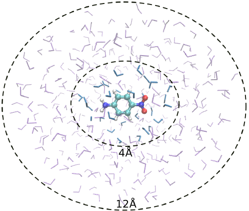
Figure 3: Example MD configuration of para-nitroaniline in a 4 Å and 12 Å water environment selection

First, we investigate environment sizes of 3 Å and 4 Å for seven snapshots. Fig. 4 shows the contributions to the total $\mathcal{S}$-shifts of pNA for the different solvent models and compare them to the supermolecular reference. It can be seen, that the total $\mathcal{S}$-shift varies largely for the different snapshots, independent of the environment size or embedding scheme used. Both, PE and FDE models reproduce the changes obtained in the reference calculations qualitatively correctly:

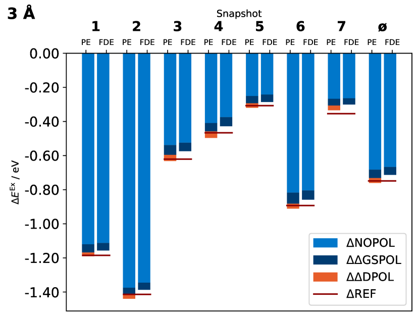
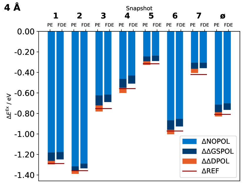
Figure 4: Contributions from the different models to the total $\mathcal{S}$-shifts and their average for different configurations of pNA in 3 and 4 Å environments of water obtained from an MD simulation and subsequently calculated in a PE and FDE framework and different orders of polarization contributions obtained in calculations with a aug-cc-pVTZ basis set.

For both, FDE and PE, $\Delta$NOPOL is the largest contribution to the $\mathcal{S}$-shift (on average a proportion of more than 86%). Thus, the GSPOL contribution ($\Delta\Delta$GSPOL) is small (7% and 9% of the supermolecular $\mathcal{S}$-shift for FDE and PE, respectively). The PE $\Delta\Delta$DPOL proportion lies below 5%. Thus, $\Delta$NOPOL and $\Delta$GSPOL for PE as well as FDE are in very good agreement with $\Delta$REF (the largest average differences are $-$0.01 eV, see tabs. S-2.3, S-2.4, S-2.7 and S-2.8 in the SI).

Ultimately, the total $\mathcal{S}$-shifts for $\Delta$GSPOL and $\Delta$DPOL are in good agreement with the $\Delta$REF (fig. 4). $\Delta$GSPOL on average slightly underestimates the total $\mathcal{S}$-shift, whereas adding the $\Delta$DPOL leads to an (equally small) overestimation: For most snapshots, the $\Delta$DPOL from PE is slightly higher than for the $\Delta$REF, with an average deviation of $-$0.01 eV and $-$0.02 eV for the 3 Å and 4 Å system, respectively (see tables S-2.3-S-2.4 in the SI for the 3 Å system and tables S-2.7-S-2.8 in the SI for the 4 Å system). These differences are smaller than differences we would expect from the differences in the applied xc functionals (the reference calculation is a full CAM-B3LYP calculation and in the determination of the PE embedding potential B3LYP was employed for environment fragments).

It should be noted that for individual snapshots, the $\Delta\Delta$GSPOL proportion can exceed the average considerably. This is most pronounced for snapshot 5, which shows an overall small total $\mathcal{S}$-shift: Here, the $\Delta\Delta$GSPOL proportion for both FDE and PE constitutes between 13% and 16% of the supermolecular $\mathcal{S}$-shift for 3 and 4 Å environments, respectively. PE $\Delta\Delta$DPOL takes a proportion of 10% and 13% in the 3 and 4 Å environments.

We further observe a slight change in the proportions when increasing the environment size: When going from 3 Å to 4 Å environment, the average $\Delta\Delta$GSPOL proportion remains around 7% of the supermolecular shift for FDE and slightly increases from 7% to 9% for PE. The PE $\Delta\Delta$DPOL proportion on average increases from 4% to 5%. In absolute values, however, these contributions for all environment sizes are rather low, i.e. at most $-$0.10 eV for $\Delta\Delta$GSPOL for both PE and FDE and $-$0.06 eV for $\Delta\Delta$DPOL in PE.

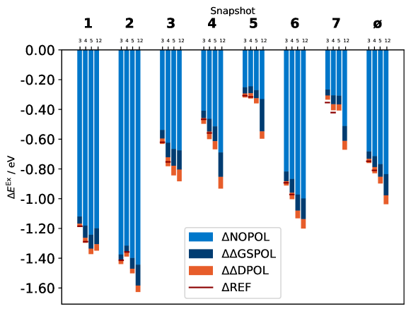
Figure 5: Contributions from the different models to the total $\mathcal{S}$-shifts and their average for different configurations of pNA in 3, 4, 5, and 12 Å environments of water obtained from an MD simulation and subsequently calculated in a PE framework and different orders of polarization contributions obtained in calculations with a aug-cc-pVTZ basis set.

For PE, we extend the environment further to 5 Å and a 12 Å. The results for the $\mathcal{S}$-shifts from all these calculations are depicted in fig. 5. The overall trend is a distinct increase in the size of the total $\mathcal{S}$-shifts when extending from a 3 Å to a 12 Å environment (i.e. the shift becomes more negative): on average it increases by $-$0.27 eV. Again, $\Delta$NOPOL is the largest contribution and it increases with enlarged environment size: With the extension from the 3 Å to 4 Å environment it increases by $-$0.02 eV on average, from the 4 Å to the 5 Å environment it increases by $-$0.06 eV on average, and by $-$0.07 eV when further extending to the 12 Å environment. $\Delta\Delta$GSPOL also increases: the increase is on average $-$0.02 eV from the 3 Å to 4 Å environment, additional $-$0.02 eV from the 4 Å to the 5 Å environment, and $-$0.05 eV when extending to the 12 Å environment. $\Delta\Delta$DPOL also shows an increase when going from a 3 Å to a 12 Å environment. The absolute contribution on average increases from $-$0.03 eV to $-$0.06 eV. However, the average proportion of the total shift does not steadily increase: From a 3 to a 4 Å environment it changes from $-$0.03 eV (4% of $\Delta$DPOL) to $-$0.04 eV (5% of $\Delta$DPOL), for a 5 Å environment it decreases to $-$0.04 eV (4% of $\Delta$DPOL) and increases for a 12 Å environment to $-$0.06 eV (6% of $\Delta$DPOL).
As discussed above, for the snapshots with smaller total shifts, $\Delta\Delta$GSPOL can exceed the average considerably: Here, we again look at snapshot 5 for which the $\Delta\Delta$GSPOL proportion changes from 13% ($-$0.05 eV ) in a 3 Å environment to 15% ($-$0.05 eV) in a 4 Å environment, 14% ($-$0.05 eV) in a 5 Å environment, and 37% ($-$0.22 eV) in a 12 Å environment, where all percentages refer to the $\Delta$ DPOL shift. Thus, for this particular snapshot, the $\Delta$NOPOL accounts for 55% ($-$0.33 eV) of $\Delta$DPOL for a 12 Å environment model.

According to previous studies on pNA in a water environment with an EOM-CCSD/EFP scheme, Slipchenko et al.[39] found the $\Delta$NOPOL proportion of the excitation energy to be of similar amount (80%) as was obtained in our calculations (86–88%). The $\Delta\Delta$DPOL proportion was determined to be 3–8% which is in good agreement with our result of 4–5%. In their study, increasing the number of water molecules used in the solvation (2–6 molecules) led to an increase in $\Delta\Delta$DPOL, similar to the increase observed in our results.
In a study by Sneskov et al.[40], the average polarization contribution was obtained from 100 snapshots. Both the $\Delta\Delta$GSPOL and the $\Delta\Delta$DPOL proportion are higher than in the present study’s result: 19-21% and 13% for the $\Delta\Delta$GSPOL and $\Delta\Delta$DPOL proportion, respectively. These authors also noted that the variation of these values is partially dependent on the individual snapshot. In and FDE context, absolute values for $\Delta\Delta$DPOL were obtained from mutual optimization with excited-state densities a the study of Daday et al.[8]. The magnitudes (0.01–0.22 or $-$0.02–0.15 eV, depending on the description of the excited-state density) are similar to our results for $\Delta\Delta$DPOL ranging between 0.02–0.06 eV.

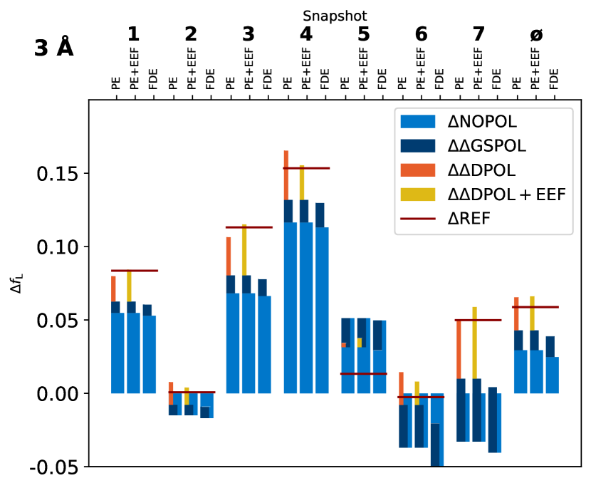
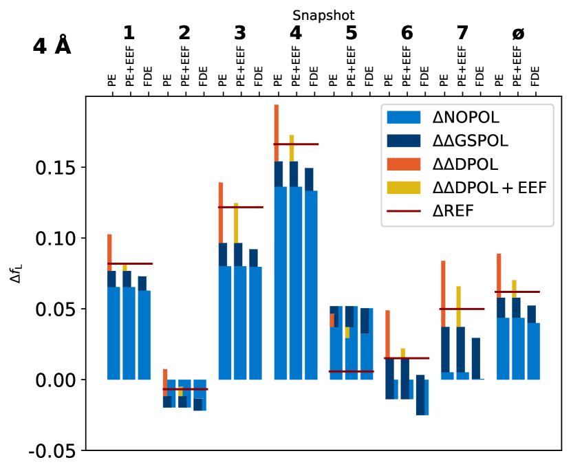
Figure 6: Contributions from the different models to the total $\mathcal{F}$-shifts and their average for different configurations of pNA in 3 and 4 Å environments of water obtained from an MD simulation and subsequently calculated in a PE and FDE framework, different orders of polarization contributions and added EEF effects obtained in calculations with a aug-cc-pVTZ basis set. (Full data in tabs. S-2.15, S-2.16, S-2.19, S-2.20)

Equivalently to the $\mathcal{S}$-shifts discussed above, fig. 6 displays the change in the oscillator strength ($\mathcal{F}$-shift) of the strongest ($\pi\rightarrow\pi^{*}$) transition for the various PE and FDE solvation models. We find that the $\mathcal{F}$-shift of the reference calculations displays larger sensitivity than the $\mathcal{S}$-shifts with respect to both, the size of the system and snapshot. This is in line with previous comparisons of different electronic structure methods, showing oscillator strengths to be more sensitive to the employed electronic structure methods[126].

In contrast to the discussion of $\mathcal{S}$-shifts, we here omit the presentation of single contributions ($\Delta$NOPOL, $\Delta\Delta$GSPOL, and $\Delta\Delta$DPOL) as percentage of the total shift since the oscillator strengths are generally smaller than the excitations energies and even small changes can lead to large percent-wise changes.
The reference $\mathcal{F}$-shifts are on average 0.06 for both 3 and 4 Å. The FDE and PE NOPOL models both give an average $\mathcal{F}$-shift of 0.03 for 3 Å and 0.04 for 4 Å. Generally, $\Delta$NOPOL is estimated similarly by FDE and PE, the largest deviation being 0.01. $\Delta$NOPOL is often the largest contribution to the total $\mathcal{F}$-shift, but is much less dominant compared to the $\mathcal{S}$-shift. Notably, the $\Delta$NOPOL results alone are often rather far from the total shifts (most obvious in snapshots 6 and 7 for both 3 and 4 Å). $\Delta\Delta$GSPOL generally improves the results for PE and FDE similarly: The largest deviation between FDE and PE amounts to less than 0.01 for both the 3 Å and 4 Å systems.

In contrast to the $\mathcal{S}$-shift, $\Delta\Delta$DPOL can be rather large for $\mathcal{F}$-shifts: In some cases (see snapshots 2 and 6) both $\Delta\Delta$GSPOL (for FDE and PE) and $\Delta\Delta$DPOL (for PE) correct the $\mathcal{F}$-shift in the opposite direction of $\Delta$NOPOL, where $\Delta$GSPOL is in better agreement with $\Delta$REF than $\Delta$DPOL. This occurs both for snapshots 2 and 6 and on average. Especially for the 4 Å environment, we observe large $\Delta$DPOL values. This over-correction of $\Delta$DPOL led us to investigate local field effects on the oscillator strength by means of effective external field (fig. 6). While for the 3 Å system on average only a small increase in $\mathcal{F}$-shift can be observed (below 0.01), the total $\mathcal{F}$-shift for the 4 Å system decreases significantly (for all snapshots), leading to an improved result compared to the reference: The average deviation is 0.03 for $\Delta$DPOL compared to and less than 0.01 for $\Delta$DPOL+EEF.

We finally note that all the discussed results are obtained with aug-cc-pVTZ but for calculations with an aug-cc-pVDZ basis set, the same trends can be observed (see figs. SI-2.2-SI-2.3 and tabs. SI-2.1-SI-2.23 in the SI). The proportions of the single contributions are in line with those obtained with an aug-cc-pVTZ basis set.

In summary, we observe similar results for FDE GSPOL and PE GSPOL, suggesting that the additional quantum-mechanical contribution and real-space treatment in FDE have only a minor effect in this case. The supermolecular reference of excitation energies of pNA in the 3 Å and 4 Å water environment is well in line with FDE results as well as the PE values with or without including differential polarization effects. When going to larger systems sizes within the PE model, we observe an increased $\Delta\Delta$GSPOL proportion to the $\mathcal{S}$-shift, but an unclear trend for the differential polarization.
The observations for the oscillator strengths are similar, though not identical to those for the electronic excitation energies. In particular, we observe a larger snapshot dependence and the differential polarization contribution in the PE calculations is larger than for the excitation energies. We further observe an overcorrection for the 4 Å environments due $\Delta\Delta$DPOL, which can be largely cancelled by accounting for local field effects (EEF).

Pentameric formyl thiophene acetic acid (pFTAA)

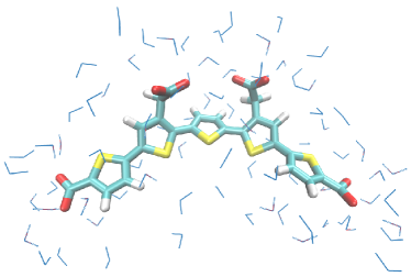
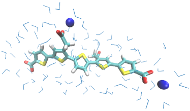
Figure 7: Selected snapshots of pFTAA in a pure 3 Å water environment (left, snapshot 1) and additionally including sodium ions in close vicinity to pFTAA (right, snapshot 2).

Table 2: Contributions from the different models to the total $\mathcal{S}$-shift $\mathcal{S}$ in eV for different configurations of pFTAA in a 3 Å environment of water obtained from an MD simulation and subsequently calculated in a PE and FDE framework and different orders of polarization contributions. Snapshots marked with ^∗ incorporate pseudopotentials in the PE calculations.

	FDE				PE						$\Delta$REF
	$\mathrm{\Delta NOPOL}$	$\mathrm{\Delta\Delta GSPOL}$	$\mathrm{\Delta GSPOL}$		$\mathrm{\Delta NOPOL}$	$\mathrm{\Delta\Delta GSPOL}$	$\mathrm{\Delta\Delta DPOL}$	$\mathrm{\Delta GSPOL}$	$\mathrm{\Delta DPOL}$
1	0.15	0.01	0.17		0.16	0.01	-0.03	0.17	0.14		0.14
2∗	0.04	0.02	0.07		0.01	0.05	-0.08	0.07	0.04		0.03

Our second test case, pFTAA, is in contrast to pNA highly negatively charged (4$-$). It is hence, more challenged by possible electron-spill-out effects, which makes it difficult to describe classical models like PE. The FDE is expected to be less prone to electron-spill-out effects due to the approximate quantum contributions in the embedding potential (c.f. eq. (6)).[127, 128] Indeed, we found that in the five snapshots that contained sodium cations close to the pFTAA chromophore, the standard PE model broke down. The electron spill-out was revealed by analyzing the contributing orbitals in the response solution vectors. We counteracted the electron spill-out in these cases by placing atomic pseudopotentials on sodium ions.[119] This led in all cases to meaningful results. The PE results for all these snapshots can be found in tabs. SI-3.2 and SI-3.4 in the SI.

Here, we focus on the discussion of two, representative snapshots: one with and one without a sodium ion in close proximity and again compare the performance of the PE and FDE models (see tab 2). Again, the supersystem reference shifts ($\Delta$REF) are well reproduced for both the FDE and PE models. $\Delta$NOPOL is by far the largest contribution, while the $\Delta\Delta$GSPOL is small. Both, $\Delta$NOPOL and $\Delta\Delta$GSPOL, are close to identical for FDE and PE. $\Delta\Delta$DPOL is of similar magnitude as $\Delta\Delta$GSPOL but points in the opposite direction.

Table 3: Contributions from the different models to the total $\mathcal{F}$-shifts for different configurations of pFTAA in a 3 Å environment of water obtained from an MD simulation and subsequently calculated in a PE and FDE framework and different orders of polarization contributions obtained with a aug-cc-pVDZ basis set. Snapshot marked with ^∗ incorporate pseudopotentials in the PE calculations

	FDE				PE								$\Delta$REF
	$\mathrm{\Delta NOPOL}$	$\mathrm{\Delta\Delta GSPOL}$	$\mathrm{\Delta TOT}_{\mathrm{GSPOL}}$		$\mathrm{\Delta NOPOL}$	$\mathrm{\Delta\Delta GSPOL}$	$\mathrm{\Delta\Delta DPOL}$	$\mathrm{\Delta\Delta EEF}$	$\mathrm{\Delta GSPOL}$	$\mathrm{\Delta DPOL}$	$\mathrm{\Delta DPOL+EEF}$
1	0.294	0.053	0.348		0.320	0.060	0.063	-0.029	0.380	0.443	0.414		0.388
2∗	0.140	0.044	0.183		0.143	0.024	0.052	-0.076	0.167	0.219	0.143		-0.007

Tab. 3 shows the $\mathcal{F}$-shifts for the PE and FDE embedding model employing the two snapshots. $\Delta$NOPOL and $\Delta\Delta$GSPOL are similar for FDE and PE, where the $\Delta\Delta$GSPOL contributions are significantly smaller than the $\Delta$NOPOL contributions. $\Delta\Delta$DPOL in the PE model for the two investigated snapshots is also rather small and of similar magnitude as the $\Delta\Delta$GSPOL contributions. The $\Delta\Delta$EEF contribution is of similar magnitude as the $\Delta\Delta$DPOL contribution but of opposing sign.
For snapshot 1, both $\Delta$GSPOL and $\Delta$DPOL are in reasonable agreement with the reference value of 0.388: For $\Delta$GSPOL we obtain deviations of 0.04 and 0.01, respectively for the FDE and the PE models. As also seen for pNA, $\Delta\Delta$DPOL overcorrects the $\mathcal{F}$-shift (leading to a deviation of 0.05 to the reference), whereas introducing EEF effects ($\Delta$DPOL+EEF) again brings the value closer to the reference.

5 Summary and Conclusions

We have investigated the influence of different approximations in classical and quantum-based embedding schemes on the excitation energies and oscillator strengths for pNA and pFTAA in different sizes of water environments. Frozen-density embedding (FDE) and polarizable embedding (PE) schemes have been compared. To enable a one-to-one comparison of these two methods, we employed an FDE framework that complies to a large degree with the PE implementation in Dalton[65, 113, 129]. In particular, we performed the mutual polarization of subsystems within FDE in the PyADF scripting environment[79, 80] using Dalton[82] for all (TD-)DFT calculations.

With this computational setup at hand, we performed a detailed analysis of the different contributions, i.e., static electrostatics (no polarization), ground-state polarization, differential polarization, and quantum-mechanical effects in the FDE and PE model to the solvent shift of pNA and pFTAA in an explicit water solvent. We compared the obtained excitation energies and oscillator strengths to supermolecular TDDFT calculations.

We find that FDE and PE perform similarly with the inclusion of static environmental densities and ground-state polarization, respectively. Since these two contributions are dominating the solvochromatic ($\mathcal{S}$-)shift for both pNA and pFTAA, FDE and PE both achieve good agreement with the reference $\mathcal{S}$-shifts. This also holds when neglecting differential polarization effects.

The effect of differential polarization on the $\mathcal{F}$-shifts seems more pronounced than that of the $\mathcal{S}$-shifts in standard PE. This effect on the $\mathcal{F}$-shifts is, however, reduced by the incorporation of external effective field effects, so that for a 4 Å environment of pNA, the average $\mathcal{F}$-shift is similarly well described with and without differential polarization. For individual snapshots, however, the effect of differential polarization can be sizeable, both with and without including external effective field effects. In these cases, external field effects improve the agreement with the supersystem reference. We could further show that the severe electron-spill-out issues preventing traditional PE calculations on the highly anionic pFTAA dye with sodium ions in close proximity could be largely reduced by atomic pseudopotentials on the sodium ions.

All in all, we find a similar performance for FDE and PE on excitation energies as well as average oscillator strengths. Accurate oscillator strengths with PE, however, required the incorporation of external effective field effects. For the anionic pFTAA example, further effective core potentials on nearby cations were essential to avoid electron-spill-out effects.

Author contributions

MJ: Methodology, Software, Validation, Formal Analysis, Investigation, Data Curation, Writing-Original Draft, Visualization; PR: Molecular Dynamics for pNA in water; EDH: Conceptualization, Validation, Formal Analysis, Writing - Review & Editing; CK: Conceptualization, Validation, Formal Analysis, Writing - Review & Editing, Supervision, Project Administration.

References

- [1] A. Warshel and M. Levitt “Theoretical Studies of Enzymic Reactions: Dielectric, Electrostatic and Steric Stabilization of the Carbonium Ion in the Reaction of Lysozyme” In J. Mol. Biol. 103.2 Academic Press, 1976, pp. 227–249 DOI: 10.1016/0022-2836(76)90311-9
- [2] U. Singh and Peter A. Kollman “A Combined Ab Initio Quantum Mechanical and Molecular Mechanical Method for Carrying out Simulations on Complex Molecular Systems: Applications to the CH3Cl + Cl- Exchange Reaction and Gas Phase Protonation of Polyethers” In J. Comput. Chem. 7.6, 1986, pp. 718–730 DOI: 10.1002/jcc.540070604
- [3] Martin J. Field, Paul A. Bash and Martin Karplus “A Combined Quantum Mechanical and Molecular Mechanical Potential for Molecular Dynamics Simulations” In J. Comput. Chem. 11.6, 1990, pp. 700–733 DOI: 10.1002/jcc.540110605
- [4] Hans Martin Senn and Walter Thiel “QM/MM Methods for Biomolecular Systems” In Angew Chem. - Int Ed 48.7 Wiley, 2009, pp. 1198–1229 DOI: 10.1002/anie.200802019
- [5] Mark A. Thompson “QM/MMpol: A Consistent Model for Solute/Solvent Polarization. Application to the Aqueous Solvation and Spectroscopy of Formaldehyde, Acetaldehyde, and Acetone” In J. Phys. Chem. 100.34 ACS Publications, 1996, pp. 14492–14507 DOI: 10.1021/jp960690m
- [6] Carles Curutchet et al. “Electronic Energy Transfer in Condensed Phase Studied by a Polarizable QM/MM Model” In J. Chem. Theory Comput. 5.7, 2009, pp. 1838–1848 DOI: 10.1021/ct9001366
- [7] Albert Defusco et al. “Modeling Solvent Effects on Electronic Excited States” In J. Phys. Chem. Lett. 2.17, 2011, pp. 2184–2192 DOI: 10.1021/jz200947j
- [8] Csaba Daday et al. “State-Specific Embedding Potentials for Excitation-Energy Calculations” In J. Chem. Theory Comput. 9.5, 2013, pp. 2355–2367 DOI: 10.1021/ct400086a
- [9] Eliot Boulanger and Jeremy N Harvey “QM/MM Methods for Free Energies and Photochemistry” In Curr. Opin. Struct. Biol. 49, 2018, pp. 72–76 DOI: 10.1016/j.sbi.2018.01.003
- [10] Mark A Thompson and Gregory K Schenter “Excited States of the Bacteriochlorophyll b Dimer of Rhodopseudomonas Viridis: A QM/MM Study of the Photosynthetic Reaction Center That Includes MM Polarization” In J. Phys. Chem. 99.17 ACS Publications, 1995, pp. 6374–6386
- [11] Jiali Gao and Kyoungrim Byun “Solvent Effects on the N$* Transition of Pyrimidine in Aqueous Solution” In Theor. Chem. Acc. 96 Springer, 1997, pp. 151–156
- [12] Hai Lin and Donald G Truhlar “QM/MM: What Have We Learned, Where Are We, and Where Do We Go from Here?” In Theor. Chem. Acc. 117.2 Springer, 2007, pp. 185–199
- [13] Nanna Holmgaard List, Jógvan Magnus Haugaard Olsen and Jacob Kongsted “Excited States in Large Molecular Systems through Polarizable Embedding” In Phys. Chem. Chem. Phys. 18.30 The Royal Society of Chemistry, 2016, pp. 20234–20250 DOI: 10.1039/c6cp03834d
- [14] Mattia Bondanza et al. “Polarizable Embedding QM/MM: The Future Gold Standard for Complex (Bio)Systems? ${\$}” In Phys. Chem. Chem. Phys 22.26 The Royal Society of Chemistry, 2020, pp. 14433 DOI: 10.1039/d0cp02119a
- [15] Daniele Loco, Louis Lagardère, Olivier Adjoua and Jean Philip Piquemal “Atomistic Polarizable Embeddings: Energy, Dynamics, Spectroscopy, and Reactivity” In Acc. Chem. Res. 54.13 American Chemical Society, 2021, pp. 2812–2822 DOI: 10.1021/acs.accounts.0c00662
- [16] Filippo Lipparini and Benedetta Mennucci “Hybrid QM/Classical Models: Methodological Advances and New Applications” In Chem. Phys. Rev. 2.4 AIP Publishing LLCAIP Publishing, 2021, pp. 041303 DOI: 10.1063/5.0064075
- [17] Marina Jansen, Thi Minh Nghia Nguyen, Erik Donovan Hedegård and Carolin König “Quantum-Derived Embedding Schemes for Local Optical Spectra” In SPR Chem. Model. The Royal Society of Chemistry, 2022, pp. 24–60 DOI: 10.1039/9781839169342
- [18] Lasse Jensen, Piet Th Van Duijnen and Jaap G. Snijders “A Discrete Solvent Reaction Field Model for Calculating Frequency-Dependent Hyperpolarizabilities of Molecules in Solution” In J. Chem. Phys. 119.24 American Institute of Physics, 2003, pp. 12998–13006 DOI: 10.1063/1.1627760
- [19] Lasse Jensen, Piet Th Van Duijnen and Jaap G. Snijders “A Discrete Solvent Reaction Field Model within Density Functional Theory” In J. Chem. Phys. 118.2 {AIP} Publishing, 2003, pp. 514–521 DOI: 10.1063/1.1527010
- [20] Jógvan Magnus Olsen, Kȩstutis Aidas and Jacob Kongsted “Excited States in Solution through Polarizable Embedding” In J. Chem. Theory Comput. 6.12 ACS Publications, 2010, pp. 3721–3734 DOI: 10.1021/ct1003803
- [21] Mark S. Gordon, Lyudmilla Slipchenko, Hui Li and Jan H. Jensen “Chapter 10 the Effective Fragment Potential: A General Method for Predicting Intermolecular Interactions” In Annu. Rep. Comput. Chem. 3 Elsevier, 2007, pp. 177–193 DOI: 10.1016/S1574-1400(07)03010-1
- [22] Mark S. Gordon, Quentin A. Smith, Peng Xu and Lyudmila V. Slipchenko “Accurate First Principles Model Potentials for Intermolecular Interactions” In Annu. Rev. Phys. Chem. 64 Annual Reviews, 2013, pp. 553–578 DOI: 10.1146/annurev-physchem-040412-110031
- [23] Daniele Loco et al. “A QM/MM Approach Using the AMOEBA Polarizable Embedding: From Ground State Energies to Electronic Excitations” In J. Chem. Theory Comput. 12.8 American Chemical Society, 2016, pp. 3654–3661 DOI: 10.1021/acs.jctc.6b00385
- [24] Weitao Yang “Direct Calculation of Electron Density in Density-Functional Theory” In Phys. Rev. Lett. 66.11 APS, 1991, pp. 1438
- [25] G. Senatore and K.. Subbaswamy “Density Dependence of the Dielectric Constant of Rare-Gas Crystals” In Phys. Rev. B 34.8 American Physical Society, 1986, pp. 5754–5757 DOI: 10.1103/PhysRevB.34.5754
- [26] M.. Johnson, K.. Subbaswamy and G. Senatore “Hyperpolarizabilities of Alkali Halide Crystals Using the Local-Density Approximation” In Phys. Rev. B 36.17, 1987, pp. 9202–9211 DOI: 10.1103/PhysRevB.36.9202
- [27] Pietro Cortona “Self-Consistently Determined Properties of Solids without Band-Structure Calculations” In Phys. Rev. B 44.16 American Physical Society, 1991, pp. 8454–8458 DOI: 10.1103/PhysRevB.44.8454
- [28] Christoph R. Jacob and Johannes Neugebauer “Subsystem Density-Functional Theory” In WIREs Comput. Mol. Sci. 4.4, 2014, pp. 325–362 DOI: 10.1002/wcms.1175
- [29] Tomasz Adam Wesolowski and Arieh Warshel “Frozen Density Functional Approach for Ab Initio Calculations of Solvated Molecules” In J. Phys. Chem. 97.30 ACS Publications, 1993, pp. 8050–8053 DOI: 10.1021/j100132a040
- [30] S Laricchia, E Fabiano, L A Constantin and F Della Sala “Generalized Gradient Approximations of the Noninteracting Kinetic Energy from the Semiclassical Atom Theory: Rationalization of the Accuracy of the Frozen Density Embedding Theory for Nonbonded Interactions” In J. Chem. Theory Comput. 7, 2011, pp. 2439–2451 DOI: 10.1021/ct200382w
- [31] Claudia Filippi, Francesco Buda, Leonardo Guidoni and Adalgisa Sinicropi “Bathochromic Shift in Green Fluorescent Protein: A Puzzle for QM/MM Approaches” In J. Chem. Theory Comput. 8.1, 2012, pp. 112–124 DOI: 10.1021/ct200704k
- [32] Csaba Daday et al. “Chromophore-Protein Coupling beyond Nonpolarizable Models: Understanding Absorption in Green Fluorescent Protein” In J. Chem. Theory Comput. 11.10, 2015, pp. 4825–4839 DOI: 10.1021/acs.jctc.5b00650
- [33] Tobias Schwabe, Maarten T.P. Beerepoot, Jógvan Magnus Haugaard Olsen and Jacob Kongsted “Analysis of Computational Models for an Accurate Study of Electronic Excitations in GFP” In Phys. Chem. Chem. Phys. 17.4 Royal Society of Chemistry, 2015, pp. 2582–2588 DOI: 10.1039/c4cp04524f
- [34] Jógvan Magnus Haugaard Olsen and Jacob Kongsted “Molecular Properties through Polarizable Embedding” In Adv. Quantum Chem. 61, Advances in Quantum Chemistry Academic Press, 2011, pp. 107–143 DOI: 10.1016/B978-0-12-386013-2.00003-6
- [35] Christoph R. Jacob, Johannes Neugebauer, Lasse Jensen and Lucas Visscher “Comparison of Frozen-Density Embedding and Discrete Reaction Field Solvent Models for Molecular Properties” In Phys. Chem. Chem. Phys. 8.20 The Royal Society of Chemistry, 2006, pp. 2349–2359 DOI: 10.1039/b601997h
- [36] André Severo Pereira Gomes et al. “Quantum-Chemical Embedding Methods for Treating Local Electronic Excitations in Complex Chemical Systems” In Annu Rep. Prog Chem - Sect C 108, 2012, pp. 222–277 DOI: 10.1039/c2pc90007f
- [37] T Fujisawa, M Terazima, Y Kimura and M Maroncelli “Resonance Raman Study of the Solvation of P-Nitroaniline in Supercritical Water” In Chem. Phys. Lett. 430.4, 2006, pp. 303–308 DOI: 10.1016/j.cplett.2006.09.019
- [38] Dmytro Kosenkov and Lyudmila V. Slipchenko “Solvent Effects on the Electronic Transitions of P-Nitroaniline: A QM/EFP Study” In J. Phys. Chem. A 115.4 American Chemical Society, 2011, pp. 392–401 DOI: 10.1021/jp110026c
- [39] Lyudmila V. Slipchenko “Solvation of the Excited States of Chromophores in Polarizable Environment: Orbital Relaxation versus Polarization” In J. Phys. Chem. A 114.33 American Chemical Society, 2010, pp. 8824–8830 DOI: 10.1021/jp101797a
- [40] Kristian Sneskov, Tobias Schwabe, Ove Christiansen and Jacob Kongsted “Scrutinizing the Effects of Polarization in QM/MM Excited State Calculations” In Phys. Chem. Chem. Phys. 13.41 The Royal Society of Chemistry, 2011, pp. 18551–18560 DOI: 10.1039/c1cp22067e
- [41] Therése Klingstedt et al. “Distinct Spacing between Anionic Groups: An Essential Chemical Determinant for Achieving Thiophene-Based Ligands to Distinguish ${\$}-Amyloid or Tau Polymorphic Aggregates” In Chem. (Easton). 21.25 Wiley-Blackwell, 2015, pp. 9072
- [42] Jonas Sjöqvist, Mathieu Linares, Mikael Lindgren and Patrick Norman “Molecular Dynamics Effects on Luminescence Properties of Oligothiophene Derivatives: A Molecular Mechanics–Response Theory Study Based on the CHARMM Force Field and Density Functional Theory” In Phys. Chem. Chem. Phys. 13.39 Royal Society of Chemistry, 2011, pp. 17532–17542
- [43] Jonas Sjöqvist, Mathieu Linares, Kurt V. Mikkelsen and Patrick Norman “QM/MM-MD Simulations of Conjugated Polyelectrolytes: A Study of Luminescent Conjugated Oligothiophenes for Use as Biophysical Probes” In J. Phys. Chem. A 118.19 American Chemical Society, 2014, pp. 3419–3428 DOI: 10.1021/jp5009835
- [44] Camilla Gustafsson, Mathieu Linares and Patrick Norman “Quantum Mechanics/Molecular Mechanics Density Functional Theory Simulations of the Optical Properties Fingerprinting the Ligand-Binding of Pentameric Formyl Thiophene Acetic Acid in Amyloid-$(1-42)” In J. Phys. Chem. A 124.5 American Chemical Society, 2020, pp. 875–888 DOI: 10.1021/acs.jpca.9b09779
- [45] Camilla Gustafsson et al. “Deciphering the Electronic Transitions of Thiophene-Based Donor-Acceptor-Donor Pentameric Ligands Utilized for Multimodal Fluorescence Microscopy of Protein Aggregates” In ChemPhysChem 22.3, 2021, pp. 323–335 DOI: 10.1002/cphc.202000669
- [46] Tomasz A. Wesolowski, Sapana Shedge and Xiuwen Zhou “Frozen-Density Embedding Strategy for Multilevel Simulations of Electronic Structure” In Chem. Rev. 115.12 American Chemical Society, 2015, pp. 5891–5928 DOI: 10.1021/cr500502v
- [47] Alisa Krishtal, Debalina Sinha, Alessandro Genova and Michele Pavanello “Subsystem Density-Functional Theory as an Effective Tool for Modeling Ground and Excited States, Their Dynamics and Many-Body Interactions” In J. Phys. Condens. Matter 27.18 IOP Publishing, 2015, pp. 183202 DOI: 10.1088/0953-8984/27/18/183202
- [48] Qiming Sun and Garnet Kin Lic Chan “Quantum Embedding Theories” In Acc. Chem. Res. 49.12 American Chemical Society, 2016, pp. 2705–2712 DOI: 10.1021/acs.accounts.6b00356
- [49] Jason D. Goodpaster, Nandini Ananth, Frederick R. Manby and Thomas F. Miller “Exact Nonadditive Kinetic Potentials for Embedded Density Functional Theory” In J. Chem. Phys. 133.8 American Institute of PhysicsAIP, 2010, pp. 84103 DOI: 10.1063/1.3474575
- [50] Frederick R. Manby, Martina Stella, Jason D. Goodpaster and Thomas F. Miller “A Simple, Exact Density-Functional-Theory Embedding Scheme” In J. Chem. Theory Comput. 8.8 American Chemical Society, 2012, pp. 2564–2568 DOI: 10.1021/ct300544e
- [51] Yuriy G. Khait and Mark R. Hoffmann “On the Orthogonality of Orbitals in Subsystem Kohn-Sham Density Functional Theory” In Annu. Rep. Comput. Chem. 8 Elsevier, 2012, pp. 53–70 DOI: 10.1016/B978-0-444-59440-2.00003-X
- [52] Dhabih V. Chulhai and Lasse Jensen “Frozen Density Embedding with External Orthogonality in Delocalized Covalent Systems” In J. Chem. Theory Comput. 11.7 American Chemical Society, 2015, pp. 3080–3088 DOI: 10.1021/acs.jctc.5b00293
- [53] Bence Hégely, Péter R. Nagy, György G. Ferenczy and Mihály Kállay “Exact Density Functional and Wave Function Embedding Schemes Based on Orbital Localization” In J. Chem. Phys. 145.6 AIP Publishing LLCAIP Publishing, 2016, pp. 64107 DOI: 10.1063/1.4960177
- [54] Dhabih V. Chulhai and Jason D. Goodpaster “Improved Accuracy and Efficiency in Quantum Embedding through Absolute Localization” In J. Chem. Theory Comput. 13.4 American Chemical Society, 2017, pp. 1503–1508 DOI: 10.1021/acs.jctc.7b00034
- [55] Tanner Culpitt, Kurt R Brorsen and Sharon Hammes-Schiffer “Communication: Density Functional Theory Embedding with the Orthogonality Constrained Basis Set Expansion Procedure” In J. Chem. Phys. 146.10, 2017, pp. 100201 DOI: 10.1063/1.4978399
- [56] Feizhi Ding, Frederick R. Manby and Thomas F. Miller “Embedded Mean-Field Theory with Block-Orthogonalized Partitioning” In J. Chem. Theory Comput. 13.4 American Chemical Society, 2017, pp. 1605–1615 DOI: 10.1021/acs.jctc.6b01065
- [57] Sebastian J.R. Lee, Matthew Welborn, Frederick R. Manby and Thomas F. Miller “Projection-Based Wavefunction-in-DFT Embedding” In Acc. Chem. Res. 52.5 American Chemical Society, 2019, pp. 1359–1368 DOI: 10.1021/acs.accounts.8b00672
- [58] Daniel S. Graham, Xuelan Wen, Dhabih V. Chulhai and Jason D. Goodpaster “Robust, Accurate, and Efficient: Quantum Embedding Using the Huzinaga Level-Shift Projection Operator for Complex Systems” In J. Chem. Theory Comput. 16.4 American Chemical Society, 2020, pp. 2284–2295 DOI: 10.1021/acs.jctc.9b01185
- [59] Daniel S. Graham, Xuelan Wen, Dhabih V. Chulhai and Jason D. Goodpaster “Huzinaga Projection Embedding for Efficient and Accurate Energies of Systems with Localized Spin-Densities” In J. Chem. Phys. 156.5 AIP Publishing LLCAIP Publishing, 2022, pp. 54112 DOI: 10.1063/5.0076493
- [60] Moritz Bensberg and Johannes Neugebauer “Automatic Basis-Set Adaptation in Projection-Based Embedding” In J. Chem. Phys. 150.18 AIP Publishing LLCAIP Publishing, 2019, pp. 184104 DOI: 10.1063/1.5084550
- [61] Moritz Bensberg and Johannes Neugebauer “Direct Orbital Selection for Projection-Based Embedding” In J. Chem. Phys. 150.21 AIP Publishing LLCAIP Publishing, 2019, pp. 214106 DOI: 10.1063/1.5099007
- [62] Tomasz Adam Wesolowski and Jacques Weber “Kohn - Sham Equations with Constrained Electron Density: An Iterative Evaluation of the Ground-State Electron Density of Interacting Molecules” In Chem. Phys. Lett. 248.1-2 North-Holland, 1996, pp. 71–76 DOI: 10.1016/0009-2614(95)01281-8
- [63] Anthony J Stone “Distributed Multipole Analysis, or How to Describe a Molecular Charge Distribution” In Chem. Phys. Lett. 83.2 Elsevier, 1981, pp. 233–239
- [64] Anthony Stone “The Theory of Intermolecular Forces” In Theory Intermol. Forces Oxford University Press, 2013 URL: https://doi.org/10.1093/acprof:oso/9780199672394.001.0001
- [65] Jógvan Magnus Haugaard Olsen and Jacob Kongsted “Molecular Properties through Polarizable Embedding” In Adv. Quantum Chem. 61 Elsevier, 2011, pp. 107–143 DOI: 10.1016/B978-0-12-386013-2.00003-6
- [66] Mark E. Casida and Tomasz A. Wesołowski “Generalization of the Kohn-Sham Equations with Constrained Electron Density Formalism and Its Time-Dependent Response Theory Formulation” In Int. J. Quantum Chem. 96.6 John Wiley & Sons, Ltd, 2004, pp. 577–588 DOI: 10.1002/qua.10744
- [67] André Severo Pereira Gomes, Christoph R. Jacob and Lucas Visscher “Calculation of Local Excitations in Large Systems by Embedding Wave-Function Theory in Density-Functional Theory” In Phys. Chem. Chem. Phys. 10.35 The Royal Society of Chemistry, 2008, pp. 5353–5362 DOI: 10.1039/b805739g
- [68] Johannes Neugebauer et al. “A Subsystem TDDFT Approach for Solvent Screening Effects on Excitation Energy Transfer Couplings” In J. Chem. Theory Comput. 6.6 American Chemical Society, 2010, pp. 1843–1851 DOI: 10.1021/ct100138k
- [69] Csaba Daday, Carolin König, Johannes Neugebauer and Claudia Filippi “Wavefunction in Density Functional Theory Embedding for Excited States: Which Wavefunctions, Which Densities?” In ChemPhysChem 15.15 WILEY-VCH Verlag, 2014, pp. 3205–3217 DOI: 10.1002/cphc.201402459
- [70] Partha Pratim Pal, Pengchong Liu and Lasse Jensen “Polarizable Frozen Density Embedding with External Orthogonalization” In J. Chem. Theory Comput. 15.12 American Chemical Society, 2019, pp. 6588–6596 DOI: 10.1021/acs.jctc.9b00472
- [71] Linus Scholz and Johannes Neugebauer “Protein Response Effects on Cofactor Excitation Energies from First Principles: Augmenting Subsystem Time-Dependent Density-Functional Theory with Many-Body Expansion Techniques” In J. Chem. Theory Comput. 17.10 American Chemical Society, 2021, pp. 6105–6121 DOI: 10.1021/ACS.JCTC.1C00551/SUPPL˙FILE/CT1C00551˙SI˙001.PDF
- [72] Aparna K. Harshan, Mark J. Bronson and Lasse Jensen “Local-Field Effects in Linear Response Properties within a Polarizable Frozen Density Embedding Method” In J. Chem. Theory Comput. 18.1 American Chemical Society, 2022, pp. 380–393 DOI: 10.1021/acs.jctc.1c00816
- [73] Jochen Autschbach and Tom Ziegler “Calculating Molecular Electric and Magnetic Properties from Time-Dependent Density Functional Response Theory” In J. Chem. Phys. 116.3 American Institute of Physics, 2002, pp. 891–896 DOI: 10.1063/1.1420401
- [74] Nanna Holmgaard List, Hans Jørgen Aagaard Jensen and Jacob Kongsted “Local Electric Fields and Molecular Properties in Heterogeneous Environments through Polarizable Embedding” In Phys. Chem. Chem. Phys. 18.15 Royal Society of Chemistry, 2016, pp. 10070–10080 DOI: 10.1039/c6cp00669h
- [75] Jógvan Magnus Haugaard Olsen et al. “PElib: The Polarizable Embedding Library”, 2020 Zenodo DOI: 10.5281/zenodo.3749733
- [76] Jógvan Magnus Haugaard Olsen, Nanna Holmgaard List and Casper Steinmann “PEAS (Polarizable Embedding Assistant Script)” In PEAS (polarizable embed. Assist. Script)
- [77] Ignacio Fdez. et al. “OpenMolcas: From Source Code to Insight” In J. Chem. Theory Comput. 15.11, 2019, pp. 5925–5964 DOI: 10.1021/acs.jctc.9b00532
- [78] Laura Gagliardi, Roland Lindh and Gunnar Karlström “Local Properties of Quantum Chemical Systems: The LoProp Approach” In J. Chem. Phys. 121.10 American Institute of Physics, 2004, pp. 4494–4500 DOI: 10.1063/1.1778131
- [79] Christoph R. Jacob et al. “PyADF - A Scripting Framework for Multiscale Quantum Chemistry” In J. Comput. Chem. 32.10 John Wiley & Sons, Ltd, 2011, pp. 2328–2338 DOI: 10.1002/jcc.21810
- [80] Christoph Jacob “PyADF Release v1.2”, 2023 Zenodo DOI: 10.5281/zenodo.3834282.
- [81] G Te Velde et al. “A.; Snijders, JG; Ziegler, t” In Chem ADF J Comput Chem 22.9, 2001, pp. 931–967
- [82] Kestutis Aidas et al. “The Dalton Quantum Chemistry Program System” In WIREs Comput. Mol. Sci. 4.3, 2014, pp. 269–284 DOI: 10.1002/wcms.1172
- [83] David A. Case et al. “The Amber Biomolecular Simulation Programs” In J. Comput. Chem. 26.16, 2005, pp. 1668–1688 DOI: 10.1002/jcc.20290
- [84] J Wang et al. “Development and Testing of a General Amber Force Field” In J. Comp. Chem. 25, 2004, pp. 1157–1174
- [85] Christopher I. Bayly, Piotr Cieplak, Wendy Cornell and Peter A. Kollman “A Well-Behaved Electrostatic Potential Based Method Using Charge Restraints for Deriving Atomic Charges: The RESP Model” In J. Phys. Chem. 97.40, 1993, pp. 10269–10280 DOI: 10.1021/j100142a004
- [86] A.. Becke “Density-Functional Exchange-Energy Approximation with Correct Asymptotic Behavior” In Phys. Rev. A 38.6 APS, 1988, pp. 3098–3100 DOI: 10.1103/PhysRevA.38.3098
- [87] Chengteh Lee, Weitao Yang and Robert G Parr “Development of the Colle-Salvetti Correlation-Energy Formula into a Functional of the Electron Density” In Phys. Rev. B 37.2 APS, 1988, pp. 785
- [88] A D Becke “Becke’s 3 Parameter Functional Combined with the Non-Local Correlation LYP J” In J. Chem. Phys. 98, 1993, pp. 5648
- [89] R. Ditchfield, W.. Hehre and J.. Pople “Self-Consistent Molecular-Orbital Methods. IX. An Extended Gaussian-Type Basis for Molecular-Orbital Studies of Organic Molecules” In J. Chem. Phys. 54.2 AIP Publishing, 1971, pp. 724–728 DOI: 10.1063/1.1674902
- [90] W.. Hehre, R. Ditchfield and J.. Pople “Self—Consistent Molecular Orbital Methods. XII. Further Extensions of Gaussian—Type Basis Sets for Use in Molecular Orbital Studies of Organic Molecules” In J. Chem. Phys. 56.5 AIP Publishing, 1972, pp. 2257–2261 DOI: 10.1063/1.1677527
- [91] Michelle M. Francl et al. “Self-Consistent Molecular Orbital Methods. XXIII. A Polarization-Type Basis Set for Second-Row Elements” In J. Chem. Phys. 77.7 AIP Publishing, 1982, pp. 3654–3665 DOI: 10.1063/1.444267
- [92] Jacopo Tomasi, Benedetta Mennucci and Roberto Cammi “Quantum Mechanical Continuum Solvation Models” In Chem. Rev. 105.8 American Chemical Society ({ACS}), 2005, pp. 2999–3093 DOI: 10.1021/cr9904009
- [93] Saeed Izadi, Ramu Anandakrishnan and Alexey V. Onufriev “Building Water Models: A Different Approach” In J. Phys. Chem. Lett. 5, 2014, pp. 3863–3871 DOI: 10.1021/jz501780a
- [94] Tom Darden, Darrin York and Lee Pedersen “Particle Mesh Ewald: An N log( N ) Method for Ewald Sums in Large Systems” In J. Chem. Phys. 98.12, 1993, pp. 10089–10092 DOI: 10.1063/1.464397
- [95] Jean-Paul Ryckaert, Giovanni Ciccotti and Herman J.C Berendsen “Numerical Integration of the Cartesian Equations of Motion of a System with Constraints: Molecular Dynamics of n-Alkanes” In J. Comput. Phys. 23.3, 1977, pp. 327–341 DOI: 10.1016/0021-9991(77)90098-5
- [96] Shuichi Miyamoto and Peter A. Kollman “Settle: An Analytical Version of the SHAKE and RATTLE Algorithm for Rigid Water Models” In J. Comput. Chem. 13.8, 1992, pp. 952–962 DOI: 10.1002/jcc.540130805
- [97] Mark James Abraham et al. “GROMACS: High Performance Molecular Simulations through Multi-Level Parallelism from Laptops to Supercomputers” In SoftwareX 1–2, 2015, pp. 19–25 DOI: 10.1016/j.softx.2015.06.001
- [98] Szilárd Páll et al. “Tackling Exascale Software Challenges in Molecular Dynamics Simulations with GROMACS” In Int. Conf. Exascale Appl. Softw., 2014, pp. 3–27 Springer
- [99] Sander Pronk et al. “GROMACS 4.5: A High-Throughput and Highly Parallel Open Source Molecular Simulation Toolkit” In Bioinformatics 29.7 Oxford University Press, 2013, pp. 845–854
- [100] Berk Hess, Carsten Kutzner, David Van Der Spoel and Erik Lindahl “GROMACS 4: Algorithms for Highly Efficient, Load-Balanced, and Scalable Molecular Simulation” In J. Chem. Theory Comput. 4.3 ACS Publications, 2008, pp. 435–447
- [101] David Van Der Spoel et al. “GROMACS: Fast, Flexible, and Free” In J. Comput. Chem. 26.16 Wiley Online Library, 2005, pp. 1701–1718
- [102] Erik Lindahl, Berk Hess and David Van Der Spoel “GROMACS 3.0: A Package for Molecular Simulation and Trajectory Analysis” In Mol. Model. Annu. 7.8 Springer, 2001, pp. 306–317
- [103] Herman J C Berendsen, David Spoel and Rudi Drunen “GROMACS: A Message-Passing Parallel Molecular Dynamics Implementation” In Comput. Phys. Commun. 91.1-3 Elsevier, 1995, pp. 43–56
- [104] Lindahl, Abraham, Hess and van Spoel “GROMACS 2019.3 Source Code”, 2019 Zenodo DOI: 10.5281/zenodo.3243833
- [105] Scott E Feller and Alexander D MacKerell “An Improved Empirical Potential Energy Function for Molecular Simulations of Phospholipids” In J. Phys. Chem. B 104.31 ACS Publications, 2000, pp. 7510–7515
- [106] Jeffery B Klauda et al. “An Ab Initio Study on the Torsional Surface of Alkanes and Its Effect on Molecular Simulations of Alkanes and a DPPC Bilayer” In J. Phys. Chem. B 109.11 ACS Publications, 2005, pp. 5300–5311
- [107] William L Jorgensen et al. “Comparison of Simple Potential Functions for Simulating Liquid Water” In J. Chem. Phys. 79.2 American Institute of Physics, 1983, pp. 926–935
- [108] Giovanni Bussi, Davide Donadio and Michele Parrinello “Canonical Sampling through Velocity Rescaling” In J. Chem. Phys. 126.1 American Institute of Physics, 2007, pp. 14101
- [109] Herman J C Berendsen et al. “Molecular Dynamics with Coupling to an External Bath” In J. Chem. Phys. 81.8 American Institute of Physics, 1984, pp. 3684–3690
- [110] ALTM Sijbers et al. “HJC Berendsen. Gromacs User Manual Version 3.0. Nijenborgh 4, 9747 AG Groningen, the Netherlands. Internet: http://www. Gromacs. Org, 2001.[4] T. Darden, D. York, and L. Pedersen. Particle Mesh Ewald: An N-log (N) Method for Ewald Sums in Large Systems. J” In Mol. Phys 52, 1984, pp. 255–268
- [111] Berk Hess, Henk Bekker, Herman J C Berendsen and Johannes G E M Fraaije “LINCS: A Linear Constraint Solver for Molecular Simulations” In J. Comput. Chem. 18.12 Wiley Online Library, 1997, pp. 1463–1472
- [112] Takeshi Yanai, David P. Tew and Nicholas C. Handy “A New Hybrid Exchange-Correlation Functional Using the Coulomb-attenuating Method (CAM-B3LYP)” In Chem. Phys. Lett. 393.1-3 North-Holland, 2004, pp. 51–57 DOI: 10.1016/j.cplett.2004.06.011
- [113] Magnus Haugaard Olsen “Development of Quantum Chemical Methods towards Rationalization and Optimal Design of Photoactive Proteins” In Univ South Den. Odense Den., 2013 URL: https://scholar.archive.org/work/pi7fyzvkcfavfnwllpzvlmfkiq/access/wayback/https://s3-eu-west-1.amazonaws.com/pfigshare-u-files/1577611/thesis%7B_%7Drev.pdf
- [114] Jan Almlöf and Peter R. Taylor “General Contraction of Gaussian Basis Sets. I. Atomic Natural Orbitals for First- and Second-Row Atoms” In J. Chem. Phys. 86.7 American Institute of Physics, 1987, pp. 4070–4077 DOI: 10.1063/1.451917
- [115] Thom H. Dunning “Gaussian Basis Sets for Use in Correlated Molecular Calculations. I. The Atoms Boron through Neon and Hydrogen” In J. Chem. Phys. 90.2 American Institute of Physics, 1989, pp. 1007–1023 DOI: 10.1063/1.456153
- [116] Rick A. Kendall, Thom H. Dunning and Robert J. Harrison “Electron Affinities of the First-Row Atoms Revisited. Systematic Basis Sets and Wave Functions” In J. Chem. Phys. 96.9, 1992, pp. 6796–6806 DOI: 10.1063/1.462569
- [117] Jógvan Magnus Haugaard Olsen, Nanna Holmgaard List, Kasper Kristensen and Jacob Kongsted “Accuracy of Protein Embedding Potentials: An Analysis in Terms of Electrostatic Potentials” In J. Chem. Theory Comput. 11.4 American Chemical Society, 2015, pp. 1832–1842 DOI: 10.1021/acs.jctc.5b00078
- [118] Rosendo Pou-Amérigo et al. “Density Matrix Averaged Atomic Natural Orbital (ANO) Basis Sets for Correlated Molecular Wave Functions - III. First Row Transition Metal Atoms” In Theor. Chim. Acta 92.3 Springer, 1995, pp. 149–181 DOI: 10.1007/BF01114922
- [119] Alireza Marefat Khah et al. “Avoiding Electron Spill-out in QM/MM Calculations on Excited States with Simple Pseudopotentials” In J. Chem. Theory Comput. 16.3 American Chemical Society, 2020, pp. 1373–1381 DOI: 10.1021/acs.jctc.9b01162
- [120] Mirko Franchini, Pierre Herman Theodoor Philipsen and Lucas Visscher “The Becke Fuzzy Cells Integration Scheme in the Amsterdam Density Functional Program Suite” In J. Comput. Chem. 34.21, 2013, pp. 1819–1827 DOI: 10.1002/jcc.23323
- [121] G Velde et al. “Chemistry with ADF” In J. Comput. Chem. 22.9 John Wiley & Sons, Inc., 2001, pp. 931–967 DOI: 10.1002/jcc.1056
- [122] John P. Perdew “Density-Functional Approximation for the Correlation Energy of the Inhomogeneous Electron Gas” In Phys. Rev. B 33.12 APS, 1986, pp. 8822–8824 DOI: 10.1103/PhysRevB.33.8822
- [123] J Perdew “Electronic Structure of Solids 91, Edited by Ziesche, P. and Eschrig, H.(Berlin: Akademie-verlag) p. 11; Perdew, JP and Wang, Y., 1992” In Phys. Rev. B 45.13, 1991, pp. 244
- [124] A Lembarki and H Chermette “Obtaining a Gradient-Corrected Kinetic-Energy Functional from the Perdew-Wang Exchange Functional” In Phys. Rev. A 50.6 American Physical Society, 1994, pp. 5328–5331 DOI: 10.1103/PhysRevA.50.5328
- [125] Karin Kiewisch, Georg Eickerling, Markus Reiher and Johannes Neugebauer “Topological Analysis of Electron Densities from Kohn-Sham and Subsystem Density Functional Theory” In J. Chem. Phys. 128.4 American Institute of Physics, 2008, pp. 44114 DOI: 10.1063/1.2822966
- [126] Erik Donovan Hedegård “Assessment of Oscillator Strengths with Multiconfigurational Short-Range Density Functional Theory for Electronic Excitations in Organic Molecules” In Mol. Phys. 115.1-2 Taylor & Francis, 2017, pp. 26–38 DOI: 10.1080/00268976.2016.1177664
- [127] Eugene V. Stefanovich and Thanh N. Truong “Embedded Density Functional Approach for Calculations of Adsorption on Ionic Crystals” In J. Chem. Phys. 104.8, 1996, pp. 2946–2955 DOI: 10.1063/1.471115
- [128] Alessandro Laio, Joost VandeVondele and Ursula Rothlisberger “A Hamiltonian Electrostatic Coupling Scheme for Hybrid Car-Parrinello Molecular Dynamics Simulations” In J. Chem. Phys. 116.16, 2002, pp. 6941–6947 DOI: 10.1063/1.1462041
- [129] Bin Gao, Andreas J Thorvaldsen and Kenneth Ruud “Gen1Int: A Unified Procedure for the Evaluation of One-Electron Integrals over Gaussian Basis Functions and Their Geometric Derivatives” In Int. J. Quantum Chem. 111.4 Wiley Online Library, 2011, pp. 858–872