Indiscernible Object Counting in Underwater Scenes

Abstract

Recently, indiscernible scene understanding has attracted a lot of attention in the vision community. We further advance the frontier of this field by systematically studying a new challenge named indiscernible object counting (IOC), the goal of which is to count objects that are blended with respect to their surroundings. Due to a lack of appropriate IOC datasets, we present a large-scale dataset IOCfish5K which contains a total of 5,637 high-resolution images and 659,024 annotated center points. Our dataset consists of a large number of indiscernible objects (mainly fish) in underwater scenes, making the annotation process all the more challenging. IOCfish5K is superior to existing datasets with indiscernible scenes because of its larger scale, higher image resolutions, more annotations, and denser scenes. All these aspects make it the most challenging dataset for IOC so far, supporting progress in this area. For benchmarking purposes, we select 14 mainstream methods for object counting and carefully evaluate them on IOCfish5K. Furthermore, we propose IOCFormer, a new strong baseline that combines density and regression branches in a unified framework and can effectively tackle object counting under concealed scenes. Experiments show that IOCFormer achieves state-of-the-art scores on IOCfish5K. The resources are available at github.com/GuoleiSun/Indiscernible-Object-Counting.

1 Introduction

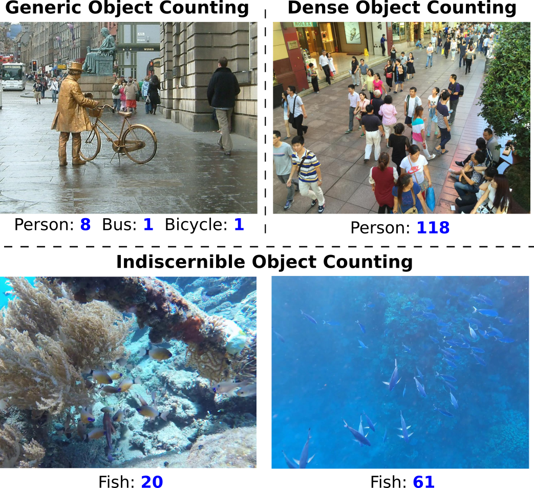
Figure 1: Illustration of different counting tasks. Top left: Generic Object Counting (GOC), which counts objects of various classes in natural scenes. Top right: Dense Object Counting (DOC), which counts objects of a foreground class in scenes packed with instances. Down: Indiscernible Object Counting (IOC), which counts objects of a foreground class in indiscernible scenes. Can you find all fishes in the given examples? For GOC, DOC, and IOC, the images shown are from PASCAL VOC [18], ShanghaiTech [91], and the new IOCfish5K dataset, respectively.

Object counting – to estimate the number of object instances in an image – has always been an essential topic in computer vision. Understanding the counts of each category in a scene can be of vital importance for an intelligent agent to navigate in its environment. The task can be the end goal or can be an auxiliary step. As to the latter, counting objects has been proven to help instance segmentation [14], action localization [54], and pedestrian detection [83]. As to the former, it is a core algorithm in surveillance [78], crowd monitoring [6], wildlife conservation [56], diet patterns understanding [55] and cell population analysis [1].

Dataset	Year	Indiscernible Scene	#Ann. IMG	Avg. Resolution	Free View	Count Statistics				Web
						Total	Min	Ave	Max
UCSD [6]	2008	✗	2,000	158$\times$238	✗	49,885	11	25	46	Link
Mall [10]	2012	✗	2,000	480$\times$640	✗	62,325	13	31	53	Link
UCF_CC_50 [27]	2013	✗	50	2101$\times$2888	✓	63,974	94	1,279	4,543	Link
WorldExpo’10 [90]	2016	✗	3,980	576$\times$720	✗	199,923	1	50	253	Link
ShanghaiTech B [91]	2016	✗	716	768$\times$1024	✗	88,488	9	123	578	Link
ShanghaiTech A [91]	2016	✗	482	589$\times$868	✓	241,677	33	501	3,139	Link
UCF-QNRF [28]	2018	✗	1,535	2013$\times$2902	✓	1,251,642	49	815	12,865	Link
Crowd_surv [87]	2019	✗	13,945	840$\times$1342	✗	386,513	2	35	1420	Link
GCC (synthetic) [80]	2019	✗	15,212	1080$\times$1920	✗	7,625,843	0	501	3,995	Link
JHU-CROWD++ [65]	2019	✗	4,372	910$\times$1430	✓	1,515,005	0	346	25,791	Link
NWPU-Crowd [79]	2020	✗	5,109	2191$\times$3209	✓	2,133,375	0	418	20,033	Link
NC4K [51]	2021	✓	4,121	530$\times$709	✓	4,584	1	1	8	Link
CAMO++ [33]	2021	✓	5,500	N/A	✓	32,756	N/A	6	N/A	Link
COD [19]	2022	✓	5,066	737$\times$964	✓	5,899	1	1	8	Link
IOCfish5K (Ours)	2023	✓	5,637	1080$\times$1920	✓	659,024	0	117	2,371	Link

Table 1: Statistics of existing datasets for dense object counting (DOC) and indiscernible object counting (IOC).

Previous object counting research mainly followed two directions: generic/common object counting (GOC) [8, 14, 32, 68] and dense object counting (DOC) [91, 28, 36, 64, 57, 50, 67]. The difference between these two sub-tasks lies in the studied scenes, as shown in Fig. 1. GOC tackles the problem of counting object(s) of various categories in natural/common scenes [8], i.e., images from PASCAL VOC [18] and COCO [41]. The number of objects to be estimated is usually small, i.e., less than 10. DOC, on the other hand, mainly counts objects of a foreground class in crowded scenes. The estimated count can be hundreds or even tens of thousands. The counted objects are often persons (crowd counting) [36, 88, 39], vehicles [57, 26] or plants [50]. Thanks to large-scale datasets [79, 91, 65, 28, 10, 18] and deep convolutional neural networks (CNNs) trained on them, significant progress has been made both for GOC and DOC. However, to the best of our knowledge, there is no previous work on counting indiscernible objects.

Under indiscernible scenes, foreground objects have a similar appearance, color, or texture to the background and are thus difficult to be detected with a traditional visual system. The phenomenon exists in both natural and artificial scenes [20, 33]. Hence, scene understanding for indiscernible scenes has attracted increasing attention since the appearance of some pioneering works [34, 20]. Various tasks have been proposed and formalized: camouflaged object detection (COD) [20], camouflaged instance segmentation (CIS) [33] and video camouflaged object detection (VCOD) [31, 12]. However, no previous research has focused on counting objects in indiscernible scenes, which is an important aspect.

In this paper, we study the new indiscernible object counting (IOC) task, which focuses on counting foreground objects in indiscernible scenes. Fig. 1 illustrates this challenge. Tasks such as image classification [24, 17], semantic segmentation [11, 42] and instance segmentation [23, 3] all owe their progress to the availability of large-scale datasets [16, 18, 41]. Similarly, a high-quality dataset for IOC would facilitate its advancement. Although existing datasets [20, 51, 33] with instance-level annotations can be used for IOC, they have the following limitations: 1) the total number of annotated objects in these datasets is limited, and image resolutions are low; 2) they only contain scenes/images with a small instance count; 3) the instance-level mask annotations can be converted to point supervision by computing the centers of mass, but the computed points do not necessarily fall inside the objects.

To facilitate the research on IOC, we construct a large-scale dataset, IOCfish5K. We collect 5,637 images with indiscernible scenes and annotate them with 659,024 center points. Compared with the existing datasets, the proposed IOCfish5K has several advantages: 1) it is the largest-scale dataset for IOC in terms of the number of images, image resolution, and total object count; 2) the images in IOCfish5K are carefully selected and contain diverse indiscernible scenes; 3) the point annotations are accurate and located at the center of each object. Our dataset is compared with existing DOC and IOC datasets in Table 1, and example images are shown in Fig. 2.

Based on the proposed IOCfish5K dataset, we provide a systematic study on 14 mainstream baselines [91, 36, 32, 47, 45, 52, 73, 76, 66, 89, 40, 39]. We find that methods which perform well on existing DOC datasets do not necessarily preserve their competitiveness on our challenging dataset. Hence, we propose a simple and effective approach named IOCFormer. Specifically, we combine the advantages of density-based [76] and regression-based [39] counting approaches. The former can estimate the object density across the image, while the latter directly regresses the coordinates of points, which is straightforward and elegant. IOCFormer contains two branches: density and regression. The density-aware features from the density branch help make indiscernible objects stand out through the proposed density-enhanced transformer encoder (DETE). Then the refined features are passed through a conventional transformer decoder, after which predicted object points are generated. Experiments show that IOCFormer outperforms all considered algorithms, demonstrating its effectiveness on IOC. To summarize, our contributions are three-fold.

• We propose the new indiscernible object counting (IOC) task. To facilitate research on IOC, we contribute a large-scale dataset IOCfish5K, containing 5,637 images and 659,024 accurate point labels.

• We select 14 classical and high-performing approaches for object counting and evaluate them on the proposed IOCfish5K for benchmarking purposes.

• We propose a novel baseline, namely IOCFormer, which integrates density-based and regression-based methods in a unified framework. In addition, a novel density-based transformer encoder is proposed to gradually exploit density information from the density branch to help detect indiscernible objects.

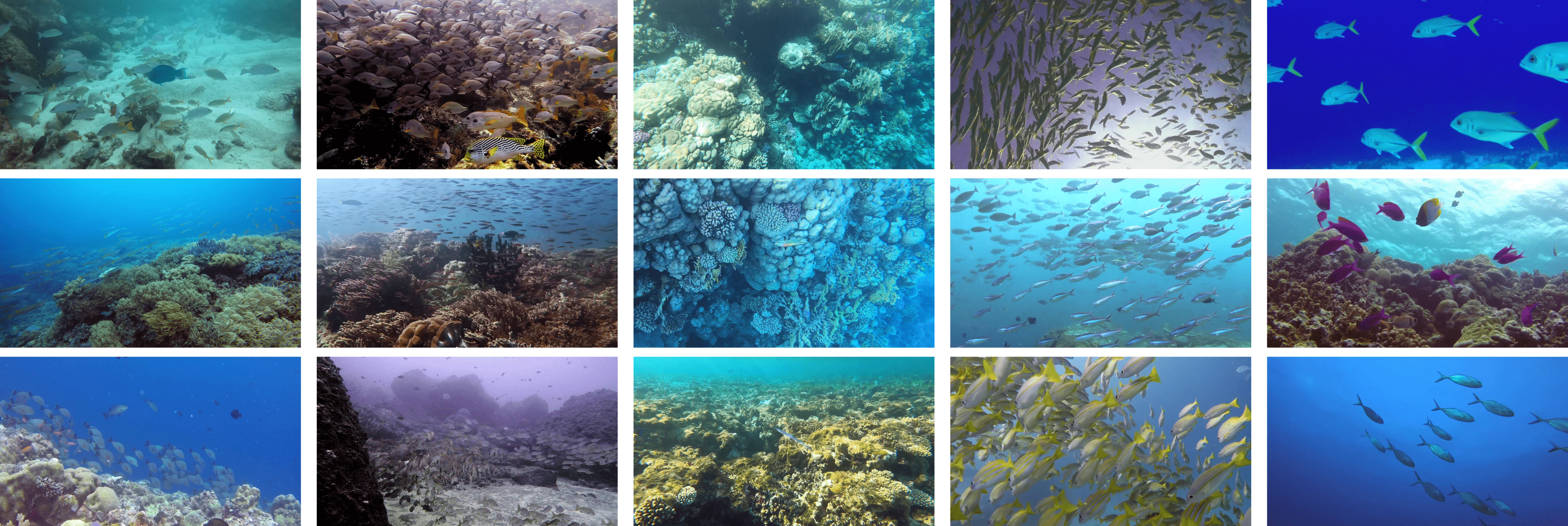
Figure 2: Example images from the proposed IOCfish5K. From left column to right column: typical samples, indiscernible & dense samples, indiscernible & less dense samples, less indiscernible & dense samples, less indiscernible & less dense samples.

2 Related Works

2.1 Generic Object Counting

Generic/common object counting (GOC) [14], also referred to as everyday object counting [8], is to count the number of object instances for various categories in natural scenes. The popular benchmarks for GOC are PASCAL VOC [18] and COCO [41]. The task was first proposed and studied in the pioneering work [8], which divided images into non-overlapping patches and predicted their counts by subitizing. LC [14] used image-level count supervision to generate a density map for each class, improving counting performance and instance segmentation. RLC [15] further reduced the supervision by only requiring the count information for a subset of training classes rather than all classes. Differently, LCFCN [32] exploited point-level supervision and output a single blob per object instance.

2.2 Dense Object Counting

Dense Object Counting (DOC) [91, 28, 84, 64, 57, 50, 53, 82, 63, 85, 13] counts the number of objects in dense scenarios. DOC contains tasks such as crowd counting [91, 28, 64, 79, 77, 37, 93, 86, 44, 29], vehicle counting [57, 26], plant counting [50], cell counting [1] and penguin counting [2]. Among them, crowd counting, i.e., counting people, attracts the most attention. The popular benchmarks for crowd counting include ShanghaiTech [91], UCF-QNRF [28], JHU-CROWD++ [64], NWPU-Crowd [79] and Mall [10]. For vehicle counting, researchers mainly use TRANCOS [57], PUCPR+ [26], and CAPRK [26]. For DOC on other categories, the available datasets are MTC [50] for counting plants, CBC [1] for counting cells, and Penguins [2] for counting penguins. DOC differs from GOC because DOC has far more objects to be counted and mainly focuses on one particular class.

Previous DOC works can be divided into three groups based on the counting strategy: detection [43, 21, 35, 61], regression [6, 7, 27, 66, 39], and density map generation [36, 47, 62, 76, 40, 69, 49]. Counting-by-detection methods first detect the objects and then count. Though intuitive, they are inferior in performance since detection performs unfavorably on crowded scenes. Counting-by-regression methods either regress the global features to the overall image count [6, 7, 27] or directly regress the local features to the point coordinates [66, 39]. Most previous efforts focus on learning a density map, which is a single-channel output with reduced spatial size. It represents the fractional number of objects at each location, and its spatial integration equals the total count of the objects in the image. The density map can be learned by using a pseudo density map generated with Gaussian kernels [36, 45, 72] or directly using a ground-truth point map [52, 76, 69].

For architectural choices, the past efforts on DOC can also be divided into CNN-based [36, 60, 47, 48, 32, 66] and Transformer-based methods [38, 69, 39]. By nature, convolutional neural networks (CNNs) have limited receptive fields and only use local information. By contrast, Transformers can establish long-range/global relationships between the features. The advantage of transformers for DOC is demonstrated by [69, 38, 59].

2.3 Indiscernible Object Counting

Recently, indiscernible scene understanding has become popular [19, 33, 34, 31, 92, 33]. It contains a set of tasks specifically focusing on detection, instance segmentation and video object detection/segmentation. It aims to analyze scenes with objects that are difficult to recognize visually [20, 31].

In this paper, we study the new task of indiscernible object counting (IOC), which lies at the intersection of dense object counting (DOC) and indiscernible scene understanding. Recently proposed datasets [51, 33, 19] for concealed scene understanding can be used as benchmarks for IOC by converting instance-level masks to points. However, they have several limitations, as discussed in §1. Therefore, we propose the first large-scale dataset for IOC, IOCfish5K.

3 The IOCfish5K Dataset

3.1 Image Collection

Underwater scenes contain many indiscernible objects (Sea Horse, Reef Stonefish, Lionfish, and Leafy Sea Dragon) because of limited visibility and active mimicry. Hence, we focus on collecting images of underwater scenes.

We started by collecting Youtube videos of underwater scenes, using general keywords (underwater scene, sea diving, deep sea scene, etc.) and category-specific ones (Cuttlefish, Mimic Octopus, Anglerfish, Stonefish, etc.). In total, we collected 135 high-quality videos with lengths from tens of seconds to several hours. Next, we kept one image in every 100 frames ($3.3$ sec) to avoid duplicates. This still leaded to a large number of images, some showing similar scenes or having low quality. Hence, at the final step of image collection, 6 professional annotators carefully reviewed the dataset and removed those unsatisfactory images. The final dataset has 5,637 images, some of which are shown in Fig. 2. This step cost a total of 200 human hours.

3.2 Image Annotation

Annotation principles.  The goal was to annotate each animal with a point at the center of its visible part. We have striven for accuracy and completeness. The former indicates that the annotation point should be placed at the object center, and each point corresponds to exactly one object instance. The latter means that no objects should be left without annotation.

Annotation tools.  To ease annotation, we developed a tool based on open-source Labelimg. It offers the following functions: generate a point annotation in an image by clicking, drag/delete the point, mark the point when encountering difficult cases, and zoom in/out. These functions help annotators to produce high-quality point annotations and to resolve ambiguities by discussing the marked cases.

Annotation process.  The whole process is split into three steps. First, all annotators (6 experts) were trained to familiarize themselves with their tasks. They were instructed about sea animals and well-annotated samples. Then each of them was asked to annotate 50 images. The annotations were checked and evaluated. When an annotator passed the evaluation, he/she could move to the next step. Second, images were distributed to 6 annotators, giving each annotator responsibility over part of the dataset. The annotators were required to discuss confusing cases and reach a consensus. Last, they checked and refined the annotations in two rounds. The second step cost 600 human hours, while each checking round in the third step cost 300 hours. The total cost of annotation process amounted to 1,200 human hours.

Datasets	# IMG (0-50)	# IMG (51-100)	# IMG (101-200)	# IMG ($>$200)	Total
NC4K [51]	4,121	0	0	0	4,121
COD [19]	5,066	0	0	0	5,066
IOCfish5K	2,663	1,000	957	1,017	5,637

Table 2: Comparison of datasets w.r.t. image distribution across various density (count) ranges. We compute the number of images for each dataset under four density ranges.

3.3 Dataset Details

The proposed IOCfish5K dataset contains 5,637 high-quality images, annotated with 659,024 points. Table 2 shows the number of images within each count range (0-50, 51-100, 101-200, and above 200). Of all images in IOCfish5K, 957 have a medium to high object density, i.e., between 101 and 200 instances. Furthermore, 1,017 images (18% of the dataset) show very dense scenes ($>200$ objects per image). To standardize the benchmarking on IOCfish5K, we randomly divide it into three non-overlapping parts: train (3,137), validation (500), and test (2,000). For each split, the distribution of images across different count ranges follows a similar distribution.

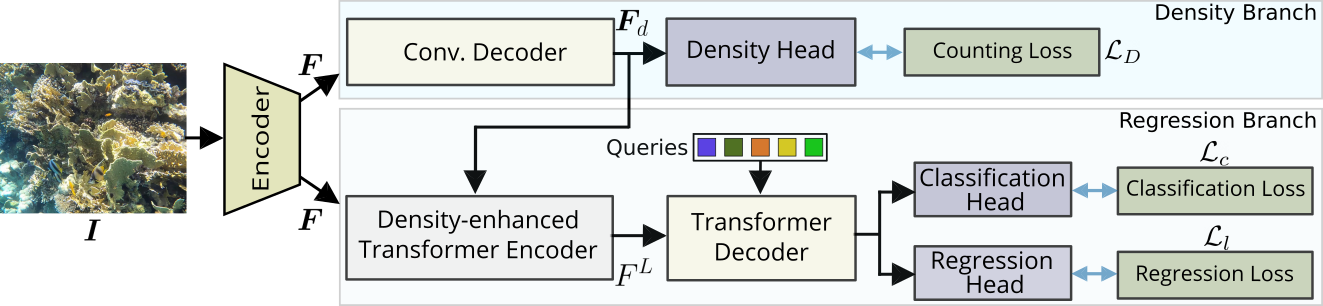
Figure 3: Overview of the proposed IOCFormer. Given an input image, we extract a feature map using an encoder, which is processed by a density branch and regression branch. The density-enhanced transformer encoder exploits the object density information from the density branch to generate more relevant features for the regression. Refer to §4 for more details.

Table 1 compares the statistics of IOCfish5K with previous datasets. The advantages of IOCfish5K over existing datasets are four-fold. (1) IOCfish5K is the largest-scale object counting dataset for indiscernible scenes. It is superior to its counterparts such as NC4K [51], CAMO++ [33], and COD [19] in terms of size, image resolution and the number of annotated points. For example, the largest existing IOC dataset CAMO++ [33] contains a total of 32,756 objects, compared to 659,024 points in IOCfish5K. (2) IOCfish5K has far denser images, which makes it currently the most challenging benchmark for IOC. As shown in Table 2, 1,974 images have more than 100 objects. (3) Although IOCfish5K is specifically proposed for IOC, it has some advantages over the existing DOC datasets. For instance, compared with JHU-CROWD++ [64], which is one of the largest-scale DOC benchmarks, the proposed dataset contains more images with a higher resolution. (4) IOCfish5K focuses on underwater scenes with sea animal annotations, which makes it different from all existing datasets shown in Table 1. Hence, the proposed dataset is also valuable for transfer learning and domain adaptation of DOC [46, 22, 9, 25].

4 IOCFormer

We first introduce the network structure of our proposed IOCFormer model, which consists of a density and a regression branch. Then, the novel density-enhanced transformer encoder, which is designed to help the network better recognize and detect indiscernible objects, is explained.

4.1 Network Structure

As mentioned, mainstream methods for object counting fall into two groups: counting-by-density [76, 36] or counting-by-regression [39, 66]. The density-based approaches [76, 36] learn a map with the estimated object density across the image. Differently, the regression-based methods [39, 66] directly regress to coordinates of object center points, which is straightforward and elegant. As for IOC, foreground objects are difficult to distinguish from the background due to their similar appearance, mainly in color and texture. The ability of density-based approaches to estimate the object density level could be exploited to make (indiscernible) foreground objects stand out and improve the performance of regression-based methods. In other words, the advantages of density-based and regression-based approaches could be combined. Thus, we propose IOCFormer, which contains two branches: a density branch and a regression branch, as in Fig. 3. The density branch’s information helps refine the regression branch’s features.

Formally, we are given an input image $\bm{I}$ with ground-truth object points $\{(x_{i},y_{i})\}_{i=1}^{K}$ where $(x_{i},y_{i})$ denotes the coordinates of the $i$-th object point and $K$ is the total number of objects. The goal is to train an object counting model which predicts the number of objects in the image. We first extract a feature map $\bm{F}\in\mathbb{R}^{h\times w\times c_{1}}$ ($h$, $w$, and $c_{1}$ denote height, weight, and the number of channels, respectively) by sending the image through an encoder. Next, $\bm{F}$ is processed by the density and the regression branches.

The density branch inputs $\bm{F}$ into a convolutional decoder which consists of two convolutions with $3\times 3$ kernels. A density-aware feature map $\bm{F}_{d}\in\mathbb{R}^{h\times w\times c_{2}}$ is obtained, where $c_{2}$ is the number of channels. Then a density head (a convolution layer with $1\times 1$ kernel and $\rm ReLU$ activation) maps $\bm{F}_{d}$ to a single-channel density map $\bm{D}\in\mathbb{R}^{h\times w}$ with non-negative values. Similar to [76], the counting loss ($L_{1}$ loss) used in the density branch is defined as:

$$\footnotesize\vspace{-2pt}\begin{split}&\mathcal{L}_{D}=\big{|}\lVert\bm{D}\rVert_{1}-K\big{|},\end{split}\vspace{-2pt}$$ (1)

where $\lVert\cdot\lVert_{1}$ denotes the entry-wise $L_{1}$ norm of a matrix. The density map $\bm{D}$ estimates the object density level across the spatial dimensions. Hence, the feature map $\bm{F}_{d}$ before the density head is density-aware and contains object density information, which could be exploited to strengthen the feature regions with indiscernible object instances.

As to the regression branch, the feature map $\bm{F}$ from the encoder and the density-aware feature map $\bm{F}_{d}$ from the density branch are first fed into our density-enhanced transformer encoder, described in detail in §4.2. After this module, the refined features, together with object queries, are passed to a typical transformer decoder [71]. The decoded query embeddings are then used by the classification head and regression head to generate predictions. The details are explained in §4.3.

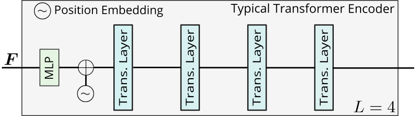
(a)

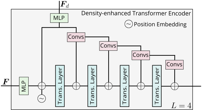
(b)

Figure 4: Comparison between typical transformer encoder (a) and our density-enhanced transformer encoder (b) when $L=4$.

4.2 Density-Enhanced Transformer Encoder

Here, we explain the density-enhanced transformer encoder (DETE) in detail. The structure of the typical transformer encoder (TTE) and the proposed DETE is shown in Fig. 4. Different from TTE, which directly processes one input, DETE takes two inputs: the features ($\bm{F}$) extracted by the initial encoder and the density-aware features ($\bm{F}_{d}$) from the density branch. DETE uses the density-aware feature map to refine the encoder feature map. With information about which image areas have densely distributed objects and which have sparsely distributed objects, the regression branch can more accurately predict the positions of indiscernible object instances.

We first project $\bm{F}$ to $\hat{\bm{F}}\in\mathbb{R}^{h\times w\times c}$, and $\bm{F}_{d}$ to $\hat{\bm{F}}_{d}\in\mathbb{R}^{h\times w\times c}$ by using an MLP layer so that the number of channels ($c$) matches. The input to the first transformer layer is the combination of $\hat{\bm{F}}$, $\hat{\bm{F}}_{d}$ and position embedding $E\in\mathbb{R}^{hw\times c}$. This process is given by:

$$\small\vspace{-2pt}\begin{split}&{F}^{1}={\rm Rs}(\hat{\bm{F}})+{\rm Rs}(\hat{\bm{F}}_{d})+E;~{}~{}F^{2}={\rm Trans}(F^{1}),\\ \end{split}\vspace{-2pt}$$ (2)

where ${\rm Rs}(\cdot)$ denotes the operation of reshaping the feature map by flattening its spatial dimensions, and ${\rm Trans}(\cdot)$ denotes a transformer layer. After that, additional transformer layers are used to further refine the features, as follows:

$$\small\vspace{-2pt}\begin{split}&\bm{F}_{d}^{1}=\hat{\bm{F}}_{d},\\ &\bm{F}_{d}^{i}={\rm Convs}(\bm{F}_{d}^{i-1}),~{}~{}i=2,3,...,L-1,\\ &F^{i+1}={\rm Trans}(F^{i}+{\rm Rs}(\bm{F}_{d}^{i})),~{}~{}i=2,3,...,L-1,\\ \end{split}\vspace{-2pt}$$ (3)

where $\rm{Convs}(\cdot)$ denotes a convolutional block containing two convolution layers. The total number of transformer layers is $L$ which also represents the total times of merging transformer and convolution features. After Equ. (3), we obtain the density-refined features $F^{L}\in\mathbb{R}^{hw\times c}$ which are forwarded to the transformer decoder.

The benefit of our DETE can also be interpreted from the perspective of global and local information. Before each transformer layer in Equ. (3), we merge features from the previous transformer layer (global) and features from the convolutional block (local). During this process, the global and local information gradually get combined, which boosts the representation ability of the module.

4.3 Loss Function

After the DETE module, we obtain density-refined features $F^{L}$. Next, the transformer decoder takes the refined features $F^{L}$ and trainable query embeddings $Q\in\mathbb{R}^{n\times c}$ containing $n$ queries as inputs, and outputs decoded embeddings $\hat{Q}\in\mathbb{R}^{n\times c}$. The transformer decoder consists of several layers, each of which contains a self-attention module, a cross-attention layer and a feed-forward network (FFN). For more details, we refer to the seminal work [71]. $\hat{Q}$ contains $n$ decoded representations, corresponding to $n$ queries. Following [39], every query embedding is mapped to a confidence score by a classification head and a point coordinate by a regression head. Let $\{p_{i},(\hat{x}_{i},\hat{y}_{i})\}_{i=1}^{n}$ denote the predictions for all queries, where $p_{i}$ is the predicted confidence score determining the likelihood that the point belongs to the foreground and $(\hat{x}_{i},\hat{y}_{i})$ is the predicted coordinate for the $i$-th query. Then we conduct a Hungarian matching [4, 39] between predictions $\{p_{i},(\hat{x}_{i},\hat{y}_{i})\}_{i=1}^{n}$ and ground-truth $\{(x_{i},y_{i})\}_{i=1}^{K}$. Note that $n$ is bigger than $K$ so that each ground-truth point has a matched prediction. The Hungarian matching is based on the $k$-nearest-neighbors matching objective [39]. Specifically, the matching cost depends on three parts: the distance between predicted points and ground-truth points, the confidence score of the predicted points, and the difference between predicted and ground-truth average neighbor distance [39]. After the matching, we compute the classification loss $\mathcal{L}_{c}$, which boosts the confidence score of the matched predictions and suppresses the confidence score of the unmatched ones. To supervise the predicted coordinates’ learning, we also compute the localization loss $\mathcal{L}_{l}$, which measures the $L_{1}$ distance between the matched predicted coordinates and the corresponding ground-truth coordinates. For more details, we refer to [39]. The final loss function is defined as:

$$\small\vspace{-2pt}\begin{split}&\mathcal{L}=\lambda\mathcal{L}_{D}+\mathcal{L}_{c}+\mathcal{L}_{l},\end{split}\vspace{-2pt}$$ (4)

where $\lambda$ is set to 0.5. The density and the regression branch are jointly trained using Equ. (4). During inference, we take the predictions from the regression branch.

		Val (500)			Test (2,000)
Method	Publication	MAE$\downarrow$	MSE$\downarrow$	NAE$\downarrow$	MAE$\downarrow$	MSE$\downarrow$	NAE$\downarrow$
MCNN [91]	CVPR’16	81.62	152.09	3.53	72.93	129.43	4.90
CSRNet [36]	CVPR’18	43.05	78.46	1.91	38.12	69.75	2.48
LCFCN [32]	ECCV’18	31.99	81.12	0.77	28.05	68.24	1.12
CAN [47]	CVPR’19	47.77	83.67	2.10	42.02	74.46	2.58
DSSI-Net [45]	ICCV’19	33.77	80.08	1.25	31.04	69.11	1.68
BL [52]	ICCV’19	19.67	44.21	0.39	20.03	46.08	0.55
NoisyCC [73]	NeurIPS’20	19.48	41.76	0.39	19.73	46.85	0.46
DM-Count [76]	NeurIPS’20	19.65	42.56	0.42	19.52	45.52	0.55
GL [74]	CVPR’21	18.13	44.57	0.33	18.80	46.19	0.47
P2PNet [66]	ICCV’21	21.38	45.12	0.39	20.74	47.90	0.48
KDMG [75]	TPAMI’22	22.79	47.32	0.90	22.79	49.94	1.17
MPS [89]	ICASSP’22	34.68	59.46	2.06	33.55	55.02	2.61
MAN [40]	CVPR’22	24.36	40.65	2.39	25.82	45.82	3.16
CLTR [39]	ECCV’22	17.47	37.06	0.29	18.07	41.90	0.43
IOCFormer (Ours)	CVPR’23	15.91	34.08	0.26	17.12	41.25	0.38

Table 3: Comparison with state-of-the-art methods on the validation and test set. The best results are highlighted in bold.

5 Experiments

5.1 Experimental Setting

Compared models.  Since there is no algorithm specifically designed for IOC, we select 14 recent open-source DOC methods for benchmarking. Selected methods include: MCNN [91], CSRNet [36], LCFCN [32], CAN [47], DSSI-Net [45], BL [52], NoisyCC [73], DM-Count [76], GL [74], P2PNet [66], KDMG [75], MPS [89], MAN [40], and CLTR [39]. Among them, P2PNet and CLTR are based on regression, while others are on density map estimation.

Implementation details.  For methods such as MCNN and CAN, we use open-source re-implementations for our experiments. For the other methods, we use official codes and default parameters. All experiments are conducted on PyTorch [58] and NVIDIA GPUs. $L$ in DETE is set to 6 and the number of queries ($n$) is set as 700. Following [39], our IOCFormer uses ResNet-50 [24] as encoder, pretrained on Imagenet [16]. Other modules/parameters are randomly initialized. For data augmentations, we use random resizing and horizontal flipping. The images are randomly cropped to $256\times 256$ inputs. Each batch contains 8 images, and the Adam optimizer [30] is used. During inference, we split the images into patches of the same size as during training. Following [39], we use a threshold (0.35) to filter out background predictions.

Metrics.  To evaluate the effectiveness of the baselines and the proposed method, we compute Mean Absolute Error (MAE), Mean Square Error (MSE), and Mean Normalized Absolute Error (NAE) between predicted counts and ground-truth counts for all images, following [76, 39, 79].

5.2 Counting Results and Analysis

We present the results of 14 mainstream crowd-counting algorithms and IOCFormer in Table 3. All methods follow the same evaluation protocol: the model is selected via the val set. Based on the results, we observe:

• Among all previous methods, the recent CLTR [39] outperforms the rest, with 18.07, 41.90, 0.43 on the test set for MAE, MSE, and NAE, respectively. The reason is that this method uses a transformer encoder to learn global information and a transformer decoder to directly predict center points for object instances.

• Some methods (MAN [40] and P2PNet [66]) perform competitively on DOC datasets such as JHU++ [65] and NWPU [79], but perform worse on IOCfish5K. For example, MAN achieves 53.4 and 209.9 for MAE and MSE on JHU++, outperforming other methods, including CLTR which achieves 59.5 and 240.6 for MAE and MSE. However, MAN underperforms on IOCfish5K, compared to CLTR, DM-Count, NoisyCC, and BL. This shows that methods designed for DOC do not necessarily work well for indiscernible objects. Hence, IOC requires specifically designed solutions.

• These methods, including BL, NoisyCC, DM-Count, and GL, which propose new loss functions for crowd counting, perform well despite being simple. For example, GL achieves 18.80, 46.19, and 0.47 for MAE, MSE, and NAE on the test set.

Different from previous methods, IOCFormer is specifically designed for IOC with two novelties: (1) combining density and regression branches in a unified framework, which improves the underlying features; (2) density-based transformer encoder, which strengthens the feature regions where objects exist. On both the val and test sets, IOCFormer is superior to all previous methods for MAE, MSE, and NAE. Besides the quantitative results, we also show qualitative results of some approaches in Fig. 5.

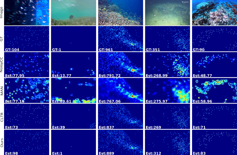
Figure 5: Qualitative comparisons of various algorithms (NoisyCC [73], MAN [40], CLTR [39], and ours). The GT or estimated counts for each case are shown in the lower left corner. Best viewed with zooming.

Methods	DETE	MAE$\downarrow$	MSE$\downarrow$	NAE$\downarrow$
DB	✗	18.25	39.77	0.29
Regression	✗	17.47	37.06	0.29
DB+Regression	✗	16.94	35.92	0.26
	✓	15.91	34.08	0.26

Table 4: Impact of density branch (DB) and DETE on IOCfish5K val set. For DB+Regression without using DETE, a typical transformer encoder (TTE) is used instead.

5.3 Ablation Study

Impact of the density branch and DETE.  As mentioned, the proposed model combines a density and a regression branch in a unified framework, aiming to combine their advantages. In Table 4, we show the results of separately training the density branch and the regression branch. We also provide results of jointly training the density branch and regression branch without using the proposed DETE. The comparison shows that the regression branch, though straightforward, performs better than only using the density branch. Furthermore, training both branches together without DETE gives better performance than using only the regression branch. The improvement could be explained from the perspective of multi-task learning [5, 81, 70]. The added density branch, which could be regarded as an additional task, helps the encoder learn better features. By establishing connections between the density and regression branches, better performance is obtained. Compared to the variant without DETE, our final model has a clear superiority by reducing MAE from 16.94 to 15.91 and MSE from 35.92 to 34.08. The results validate the effectiveness of DETE for enhancing the features by exploiting the information generated from the density branch.

$L$	MAE$\downarrow$	MSE$\downarrow$	NAE$\downarrow$
2	16.75	35.87	0.28
4	16.59	35.23	0.26
6	15.91	34.08	0.26
8	15.72	33.63	0.24

Table 5: Impact of the number of transformer layers or convolutional blocks in DETE.

Impact of $L$.  We change the number of $\rm Trans$ or $\rm Convs$ in DETE and report results in Table 5. By increasing $L$, we obtain better performance, showing the capability of our DETE to produce relevant features. We use $L=6$ in our main setting to balance complexity and performance.

6 Conclusions and Future Work

We provide a rigorous study of a new challenge named indiscernible object counting (IOC), which focuses on counting objects in indiscernible scenes. To address the lack of a large-scale dataset, we present the high-quality IOCfish5K which mainly contains underwater scenes and has point annotations located at the center of object (mainly fish) instances. A number of existing mainstream baselines are selected and evaluated on IOCfish5K, proving a domain gap between DOC and IOC. In addition, we propose a dedicated method for IOC named IOCFormer, which is equipped with two novel designs: combining a density and regression branch in a unified model and a density-enhanced transformer encoder which transfers object density information from the density to the regression branch. IOCFormer achieves SOTA performance on IOCfish5K. To sum up, our dataset and method provide an opportunity for future researchers to dive into this new task.

Future work. There are several directions. (1) To improve performance and efficiency. Although our method achieves state-of-the-art performance, there is room to further improve the counting results on IOCfish5K in terms of MAE, MSE, and NAE. Also, efficiency is important when deploying counting models in real applications. (2) To study domain adaptation among IOC and DOC. There are many more DOC datasets than IOC datasets and how to improve IOC using available DOC datasets is a practical problem to tackle. (3) To obtain a general counting model which can count everything (people, plants, cells, fish, etc.).

Appendix

A. More Details about IOCfish5K

Answers.  The ground-truth point maps of the IOC examples shown in the introduction of the main paper are presented in Fig. 6. For a normal visual system, it is difficult to find all the object (fish) instances in the given examples because some objects are highly blended in their environment. Surprisingly, there are a total of 20 and 61 objects in the two examples, respectively.

More examples.  We show more example images of IOCfish5K in Fig. 7. Our dataset contains plenty of high-quality images with various indiscernible levels and object densities. It would contribute to research areas such as indiscernible scene understanding and dense object counting.

Annotation details.  As mentioned in our main paper, the annotation process is split into three steps. For the first step, we studied books and watched Youtube videos to learn the background knowledge about sea animals before instructing annotators. The used books include Wonders of the Red Sea and Fishing guide Mediterranean + Atlantic, which are available on Amazon. We also took some examples/pictures from the above materials to instruct annotators.

B. More Experimental Details

As mentioned, we evaluated 14 popular algorithms for DOC on IOCfish5K. Their codes are all publicly available. The details of these methods are as follows.

MCNN [91]:  It proposes a multi-column convolutional neural network that contains different convolution branches with different receptive fields. The ground-truth density map is calculated using geometry-adaptive kernels.

CSRNet [36]:  It aims at conducting crowd counting under highly congested scenes. CSRNet exploits dilated convolutions in this task and achieve promising results.

LCFCN [32]:  This method predicts a blob for each object instance by using only point supervision. It achieves excellent performance in crowd counting as well as generic object counting.

CAN [47]:  CAN processes encoded features (VGG-16) with different receptive fields, which are then combined using the learned weights. The final context-aware features are passed to estimate the density map.

DSSI-Net [45]:  It focuses on tackling the problem of large-scale variation in crowd counting and proposes structured feature enhancement and dilated multi-scale structural similarity loss to generate better density maps.

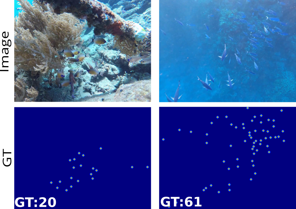
Figure 6: Ground-truth annotations, for example images shown in the introduction of the main paper. Best viewed with zooming.

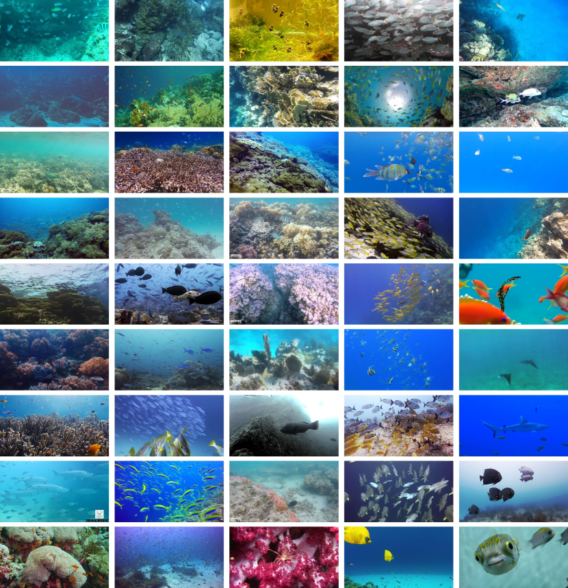
Figure 7: More example images from the proposed IOCfish5K. From left column to right column: typical samples, indiscernible & dense samples, indiscernible & less dense samples, less indiscernible & dense samples, less indiscernible & less dense samples.

BL [52]:  Different from previous works which adopt $L_{1}$ or $L_{2}$ loss for supervising the learning of density maps, BL proposes a Bayesian loss which directly uses point annotations to learn density probability.

NoisyCC [73]:  NoisyCC explicitly models the annotation noise in crowd counting with a joint Gaussian distribution. A low-rank covariance approximation is derived to improve the efficiency [73].

DM-Count [76]:  This method proposes to exploit distribution matching for crowd counting. The optimal transport algorithm is used to minimize the gap between the predicted density map and the ground-truth point map.

GL [74]:  GL proposes a perspective-guided optimal transport cost function for crowd counting. It is currently the most powerful loss for crowd counting and achieves state-of-the-art performance on mainstream DOC datasets compared to other loss functions.

P2PNet [66]:  It directly predicts a number of point proposals (location and confidence score). Then Hungarian algorithm [4] is used to match proposals and point annotations. It is a purely point-based algorithm for crowd counting [66] and achieves impressive performance on DOC datasets.

KDMG [75]:  Different from previous density-based methods, which generates ground-truth density map by convolving the point map with a/an (adaptive) Gaussian kernel, KDMG proposes a density map generator that is jointly trained with counting model.

MPS [89]:  This method generates multi-scale features for the crowd image and benefits from the joint learning of crowd counting as well as localization.

MAN [40]:  It deals with the problem of large-scale variations in crowd counting by integrating global attention, local attention, and instance attention in a unified framework. MAN achieves state-of-the-art performance on mainstream datasets such as JHU++ and NWPU.

CLTR [39]:  It directly predicts the point locations by adopting a transformer encoder and decoder structure to process the features. The trainable embeddings are used to extract object locations from the encoded features.

For the above methods, CAN, CSRNet and MCNN use the SGD optimization algorithm for training the network, while others use Adam optimizer [30]. For IOCFormer, the initial learning rate is set as 1e-5 and the weight decay is 5e-4. Following [39], our approach is trained by 1500 epochs.

References

- [1] Mohammad Mahmudul Alam and Mohammad Tariqul Islam. Machine learning approach of automatic identification and counting of blood cells. HTL, 6(4):103–108, 2019.
- [2] Carlos Arteta, Victor Lempitsky, and Andrew Zisserman. Counting in the wild. In ECCV, 2016.
- [3] Daniel Bolya, Chong Zhou, Fanyi Xiao, and Yong Jae Lee. Yolact: Real-time instance segmentation. In IEEE ICCV, 2019.
- [4] Nicolas Carion, Francisco Massa, Gabriel Synnaeve, Nicolas Usunier, Alexander Kirillov, and Sergey Zagoruyko. End-to-end object detection with transformers. In ECCV, 2020.
- [5] Rich Caruana. Multitask learning. ML, 28(1):41–75, 1997.
- [6] Antoni B Chan, Zhang-Sheng John Liang, and Nuno Vasconcelos. Privacy preserving crowd monitoring: Counting people without people models or tracking. In IEEE CVPR, 2008.
- [7] Antoni B Chan and Nuno Vasconcelos. Bayesian poisson regression for crowd counting. In IEEE ICCV, 2009.
- [8] Prithvijit Chattopadhyay, Ramakrishna Vedantam, Ramprasaath R Selvaraju, Dhruv Batra, and Devi Parikh. Counting everyday objects in everyday scenes. In IEEE CVPR, 2017.
- [9] Binghui Chen, Zhaoyi Yan, Ke Li, Pengyu Li, Biao Wang, Wangmeng Zuo, and Lei Zhang. Variational attention: Propagating domain-specific knowledge for multi-domain learning in crowd counting. In IEEE ICCV, 2021.
- [10] Ke Chen, Chen Change Loy, Shaogang Gong, and Tony Xiang. Feature mining for localised crowd counting. In BMVC, 2012.
- [11] Liang-Chieh Chen, George Papandreou, Iasonas Kokkinos, Kevin Murphy, and Alan L Yuille. Deeplab: Semantic image segmentation with deep convolutional nets, atrous convolution, and fully connected crfs. IEEE TPAMI, 40(4):834–848, 2017.
- [12] Xuelian Cheng, Huan Xiong, Deng-Ping Fan, Yiran Zhong, Mehrtash Harandi, Tom Drummond, and Zongyuan Ge. Implicit motion handling for video camouflaged object detection. In IEEE CVPR, 2022.
- [13] Zhi-Qi Cheng, Qi Dai, Hong Li, Jingkuan Song, Xiao Wu, and Alexander G. Hauptmann. Rethinking spatial invariance of convolutional networks for object counting. In IEEE CVPR, 2022.
- [14] Hisham Cholakkal, Guolei Sun, Fahad Shahbaz Khan, and Ling Shao. Object counting and instance segmentation with image-level supervision. In IEEE CVPR, 2019.
- [15] Hisham Cholakkal, Guolei Sun, Salman Khan, Fahad Shahbaz Khan, Ling Shao, and Luc Van Gool. Towards partial supervision for generic object counting in natural scenes. IEEE TPAMI, 44(3):1604–1622, 2022.
- [16] Jia Deng, Wei Dong, Richard Socher, Li-Jia Li, Kai Li, and Li Fei-Fei. Imagenet: A large-scale hierarchical image database. In IEEE CVPR, 2009.
- [17] Alexey Dosovitskiy, Lucas Beyer, Alexander Kolesnikov, Dirk Weissenborn, Xiaohua Zhai, Thomas Unterthiner, Mostafa Dehghani, Matthias Minderer, Georg Heigold, Sylvain Gelly, et al. An image is worth 16x16 words: Transformers for image recognition at scale. In ICLR, 2020.
- [18] Mark Everingham, SM Eslami, Luc Van Gool, Christopher KI Williams, John Winn, and Andrew Zisserman. The pascal visual object classes challenge: A retrospective. IJCV, 111(1):98–136, 2015.
- [19] Deng-Ping Fan, Ge-Peng Ji, Ming-Ming Cheng, and Ling Shao. Concealed object detection. IEEE TPAMI, 44(10):6024–6042, 2022.
- [20] Deng-Ping Fan, Ge-Peng Ji, Guolei Sun, Ming-Ming Cheng, Jianbing Shen, and Ling Shao. Camouflaged object detection. In IEEE CVPR, 2020.
- [21] Weina Ge and Robert T Collins. Marked point processes for crowd counting. In IEEE CVPR, 2009.
- [22] Shenjian Gong, Shanshan Zhang, Jian Yang, Dengxin Dai, and Bernt Schiele. Bi-level alignment for cross-domain crowd counting. In IEEE CVPR, 2022.
- [23] Kaiming He, Georgia Gkioxari, Piotr Dollár, and Ross Girshick. Mask r-cnn. In IEEE ICCV, 2017.
- [24] Kaiming He, Xiangyu Zhang, Shaoqing Ren, and Jian Sun. Deep residual learning for image recognition. In IEEE CVPR, 2016.
- [25] Yuhang He, Zhiheng Ma, Xing Wei, Xiaopeng Hong, Wei Ke, and Yihong Gong. Error-aware density isomorphism reconstruction for unsupervised cross-domain crowd counting. In AAAI, 2021.
- [26] Meng-Ru Hsieh, Yen-Liang Lin, and Winston H Hsu. Drone-based object counting by spatially regularized regional proposal network. In IEEE ICCV, 2017.
- [27] Haroon Idrees, Imran Saleemi, Cody Seibert, and Mubarak Shah. Multi-source multi-scale counting in extremely dense crowd images. In IEEE CVPR, 2013.
- [28] Haroon Idrees, Muhmmad Tayyab, Kishan Athrey, Dong Zhang, Somaya Al-Maadeed, Nasir Rajpoot, and Mubarak Shah. Composition loss for counting, density map estimation and localization in dense crowds. In ECCV, 2018.
- [29] Xiaoheng Jiang, Li Zhang, Mingliang Xu, Tianzhu Zhang, Pei Lv, Bing Zhou, Xin Yang, and Yanwei Pang. Attention scaling for crowd counting. In IEEE CVPR, 2020.
- [30] Diederick P Kingma and Jimmy Ba. Adam: A method for stochastic optimization. In ICLR, 2015.
- [31] Hala Lamdouar, Charig Yang, Weidi Xie, and Andrew Zisserman. Betrayed by motion: Camouflaged object discovery via motion segmentation. In ACCV, 2020.
- [32] Issam H Laradji, Negar Rostamzadeh, Pedro O Pinheiro, David Vazquez, and Mark Schmidt. Where are the blobs: Counting by localization with point supervision. In ECCV, 2018.
- [33] Trung-Nghia Le, Yubo Cao, Tan-Cong Nguyen, Minh-Quan Le, Khanh-Duy Nguyen, Thanh-Toan Do, Minh-Triet Tran, and Tam V Nguyen. Camouflaged instance segmentation in-the-wild: Dataset, method, and benchmark suite. IEEE TIP, 31:287–300, 2021.
- [34] Trung-Nghia Le, Tam V Nguyen, Zhongliang Nie, Minh-Triet Tran, and Akihiro Sugimoto. Anabranch network for camouflaged object segmentation. CVIU, 184:45–56, 2019.
- [35] Min Li, Zhaoxiang Zhang, Kaiqi Huang, and Tieniu Tan. Estimating the number of people in crowded scenes by mid based foreground segmentation and head-shoulder detection. In IEEE ICPR, 2008.
- [36] Yuhong Li, Xiaofan Zhang, and Deming Chen. CSRNet: Dilated convolutional neural networks for understanding the highly congested scenes. In IEEE CVPR, 2018.
- [37] Dongze Lian, Xianing Chen, Jing Li, Weixin Luo, and Shenghua Gao. Locating and counting heads in crowds with a depth prior. IEEE TPAMI, 44(12):9056–9072, 2022.
- [38] Dingkang Liang, Xiwu Chen, Wei Xu, Yu Zhou, and Xiang Bai. Transcrowd: weakly-supervised crowd counting with transformers. SCIS, 65(6):1–14, 2022.
- [39] Dingkang Liang, Wei Xu, and Xiang Bai. An end-to-end transformer model for crowd localization. In ECCV, 2022.
- [40] Hui Lin, Zhiheng Ma, Rongrong Ji, Yaowei Wang, and Xiaopeng Hong. Boosting crowd counting via multifaceted attention. In IEEE CVPR, 2022.
- [41] Tsung-Yi Lin, Michael Maire, Serge Belongie, James Hays, Pietro Perona, Deva Ramanan, Piotr Dollár, and C Lawrence Zitnick. Microsoft coco: Common objects in context. In ECCV, 2014.
- [42] Chenxi Liu, Liang-Chieh Chen, Florian Schroff, Hartwig Adam, Wei Hua, Alan L Yuille, and Li Fei-Fei. Auto-deeplab: Hierarchical neural architecture search for semantic image segmentation. In IEEE CVPR, 2019.
- [43] Jiang Liu, Chenqiang Gao, Deyu Meng, and Alexander G Hauptmann. Decidenet: Counting varying density crowds through attention guided detection and density estimation. In IEEE CVPR, 2018.
- [44] Liang Liu, Hao Lu, Hongwei Zou, Haipeng Xiong, Zhiguo Cao, and Chunhua Shen. Weighing counts: Sequential crowd counting by reinforcement learning. In ECCV, 2020.
- [45] Lingbo Liu, Zhilin Qiu, Guanbin Li, Shufan Liu, Wanli Ouyang, and Liang Lin. Crowd counting with deep structured scale integration network. In IEEE ICCV, 2019.
- [46] Weizhe Liu, Nikita Durasov, and Pascal Fua. Leveraging self-supervision for cross-domain crowd counting. In IEEE CVPR, 2022.
- [47] Weizhe Liu, Mathieu Salzmann, and Pascal Fua. Context-aware crowd counting. In IEEE CVPR, 2019.
- [48] Xialei Liu, Joost Van De Weijer, and Andrew D Bagdanov. Exploiting unlabeled data in CNNs by self-supervised learning to rank. IEEE TPAMI, 41(8):1862–1878, 2019.
- [49] Xiyang Liu, Jie Yang, Wenrui Ding, Tieqiang Wang, Zhijin Wang, and Junjun Xiong. Adaptive mixture regression network with local counting map for crowd counting. In ECCV, 2020.
- [50] Hao Lu, Zhiguo Cao, Yang Xiao, Bohan Zhuang, and Chunhua Shen. Tasselnet: counting maize tassels in the wild via local counts regression network. PM, 13(1):79, 2017.
- [51] Yunqiu Lyu, Jing Zhang, Yuchao Dai, Aixuan Li, Bowen Liu, Nick Barnes, and Deng-Ping Fan. Simultaneously localize, segment and rank the camouflaged objects. In IEEE CVPR, 2021.
- [52] Zhiheng Ma, Xing Wei, Xiaopeng Hong, and Yihong Gong. Bayesian loss for crowd count estimation with point supervision. In IEEE ICCV, 2019.
- [53] Chenlin Meng, Enci Liu, Willie Neiswanger, Jiaming Song, Marshall Burke, David Lobell, and Stefano Ermon. Is-count: Large-scale object counting from satellite images with covariate-based importance sampling. arXiv preprint arXiv:2112.09126, 2021.
- [54] Sanath Narayan, Hisham Cholakkal, Fahad Shahbaz Khan, and Ling Shao. 3c-net: Category count and center loss for weakly-supervised action localization. In IEEE ICCV, 2019.
- [55] Huu-Thanh Nguyen, Chong-Wah Ngo, and Wing-Kwong Chan. Sibnet: Food instance counting and segmentation. PR, 124:108470, 2022.
- [56] Mohammad Sadegh Norouzzadeh, Anh Nguyen, Margaret Kosmala, Alexandra Swanson, Meredith S Palmer, Craig Packer, and Jeff Clune. Automatically identifying, counting, and describing wild animals in camera-trap images with deep learning. PNAS, 115(25):E5716–E5725, 2018.
- [57] Daniel Onoro-Rubio and Roberto J López-Sastre. Towards perspective-free object counting with deep learning. In ECCV, 2016.
- [58] Adam Paszke, Sam Gross, Francisco Massa, Adam Lerer, James Bradbury, Gregory Chanan, Trevor Killeen, Zeming Lin, Natalia Gimelshein, Luca Antiga, et al. Pytorch: An imperative style, high-performance deep learning library. In NeurIPS, 2019.
- [59] Yifei Qian, Liangfei Zhang, Xiaopeng Hong, Carl R Donovan, and Ognjen Arandjelovic. Segmentation assisted u-shaped multi-scale transformer for crowd counting. In BMVC, 2022.
- [60] Viresh Ranjan, Hieu Le, and Minh Hoai. Iterative crowd counting. In ECCV, 2018.
- [61] Deepak Babu Sam, Skand Vishwanath Peri, Mukuntha Narayanan Sundararaman, Amogh Kamath, and R Venkatesh Babu. Locate, size, and count: accurately resolving people in dense crowds via detection. IEEE TPAMI, 43(8):2739–2751, 2020.
- [62] Zenglin Shi, Pascal Mettes, and Cees GM Snoek. Counting with focus for free. In IEEE ICCV, 2019.
- [63] Weibo Shu, Jia Wan, Kay Chen Tan, Sam Kwong, and Antoni B Chan. Crowd counting in the frequency domain. In IEEE CVPR, 2022.
- [64] Vishwanath Sindagi, Rajeev Yasarla, and Vishal MM Patel. Jhu-crowd++: Large-scale crowd counting dataset and a benchmark method. IEEE TPAMI, 44(5):2594–2609, 2022.
- [65] Vishwanath A Sindagi, Rajeev Yasarla, and Vishal M Patel. Pushing the frontiers of unconstrained crowd counting: New dataset and benchmark method. In IEEE ICCV, 2019.
- [66] Qingyu Song, Changan Wang, Zhengkai Jiang, Yabiao Wang, Ying Tai, Chengjie Wang, Jilin Li, Feiyue Huang, and Yang Wu. Rethinking counting and localization in crowds: A purely point-based framework. In IEEE ICCV, 2021.
- [67] Qingyu Song, Changan Wang, Yabiao Wang, Ying Tai, Chengjie Wang, Jilin Li, Jian Wu, and Jiayi Ma. To choose or to fuse? scale selection for crowd counting. In AAAI, 2021.
- [68] Tobias Stahl, Silvia L Pintea, and Jan C Van Gemert. Divide and count: Generic object counting by image divisions. IEEE TIP, 28(2):1035–1044, 2018.
- [69] Guolei Sun, Yun Liu, Thomas Probst, Danda Pani Paudel, Nikola Popovic, and Luc Van Gool. Boosting crowd counting with transformers. arXiv preprint arXiv:2105.10926, 2021.
- [70] Guolei Sun, Thomas Probst, Danda Pani Paudel, Nikola Popović, Menelaos Kanakis, Jagruti Patel, Dengxin Dai, and Luc Van Gool. Task switching network for multi-task learning. In IEEE ICCV, 2021.
- [71] Ashish Vaswani, Noam Shazeer, Niki Parmar, Jakob Uszkoreit, Llion Jones, Aidan N Gomez, Łukasz Kaiser, and Illia Polosukhin. Attention is all you need. In NeurIPS, 2017.
- [72] Jia Wan and Antoni Chan. Adaptive density map generation for crowd counting. In IEEE ICCV, 2019.
- [73] Jia Wan and Antoni Chan. Modeling noisy annotations for crowd counting. In NeurIPS, 2020.
- [74] Jia Wan, Ziquan Liu, and Antoni B Chan. A generalized loss function for crowd counting and localization. In IEEE CVPR, 2021.
- [75] Jia Wan, Qingzhong Wang, and Antoni B. Chan. Kernel-based density map generation for dense object counting. IEEE TPAMI, 44(3):1357–1370, 2022.
- [76] Boyu Wang, Huidong Liu, Dimitris Samaras, and Minh Hoai. Distribution matching for crowd counting. In NeurIPS, 2020.
- [77] Changan Wang, Qingyu Song, Boshen Zhang, Yabiao Wang, Ying Tai, Xuyi Hu, Chengjie Wang, Jilin Li, Jiayi Ma, and Yang Wu. Uniformity in heterogeneity: Diving deep into count interval partition for crowd counting. In IEEE ICCV, 2021.
- [78] Meng Wang and Xiaogang Wang. Automatic adaptation of a generic pedestrian detector to a specific traffic scene. In IEEE CVPR, 2011.
- [79] Qi Wang, Junyu Gao, Wei Lin, and Xuelong Li. Nwpu-crowd: A large-scale benchmark for crowd counting and localization. IEEE TPAMI, 2020.
- [80] Qi Wang, Junyu Gao, Wei Lin, and Yuan Yuan. Learning from synthetic data for crowd counting in the wild. In IEEE CVPR, 2019.
- [81] Kilian Weinberger, Anirban Dasgupta, John Langford, Alex Smola, and Josh Attenberg. Feature hashing for large scale multitask learning. In ICML, 2009.
- [82] Longyin Wen, Dawei Du, Pengfei Zhu, Qinghua Hu, Qilong Wang, Liefeng Bo, and Siwei Lyu. Detection, tracking, and counting meets drones in crowds: A benchmark. In IEEE CVPR, 2021.
- [83] Jin Xie, Hisham Cholakkal, Rao Muhammad Anwer, Fahad Shahbaz Khan, Yanwei Pang, Ling Shao, and Mubarak Shah. Count-and similarity-aware r-cnn for pedestrian detection. In ECCV, 2020.
- [84] Haipeng Xiong, Hao Lu, Chengxin Liu, Liang Liu, Zhiguo Cao, and Chunhua Shen. From open set to closed set: Counting objects by spatial divide-and-conquer. In IEEE ICCV, 2019.
- [85] Haipeng Xiong and Angela Yao. Discrete-constrained regression for local counting models. In ECCV, 2022.
- [86] Chenfeng Xu, Dingkang Liang, Yongchao Xu, Song Bai, Wei Zhan, Xiang Bai, and Masayoshi Tomizuka. Autoscale: Learning to scale for crowd counting. IJCV, 130(2):405–434, 2022.
- [87] Zhaoyi Yan, Yuchen Yuan, Wangmeng Zuo, Xiao Tan, Yezhen Wang, Shilei Wen, and Errui Ding. Perspective-guided convolution networks for crowd counting. In IEEE ICCV, 2019.
- [88] Yifan Yang, Guorong Li, Zhe Wu, Li Su, Qingming Huang, and Nicu Sebe. Weakly-supervised crowd counting learns from sorting rather than locations. In ECCV, 2020.
- [89] Mohsen Zand, Haleh Damirchi, Andrew Farley, Mahdiyar Molahasani, Michael Greenspan, and Ali Etemad. Multiscale crowd counting and localization by multitask point supervision. In IEEE ICASSP, 2022.
- [90] Cong Zhang, Kai Kang, Hongsheng Li, Xiaogang Wang, Rong Xie, and Xiaokang Yang. Data-driven crowd understanding: A baseline for a large-scale crowd dataset. IEEE TMM, 18(6):1048–1061, 2016.
- [91] Yingying Zhang, Desen Zhou, Siqin Chen, Shenghua Gao, and Yi Ma. Single-image crowd counting via multi-column convolutional neural network. In IEEE CVPR, 2016.
- [92] Yijie Zhong, Bo Li, Lv Tang, Senyun Kuang, Shuang Wu, and Shouhong Ding. Detecting camouflaged object in frequency domain. In IEEE CVPR, 2022.
- [93] Joey Tianyi Zhou, Le Zhang, Jiawei Du, Xi Peng, Zhiwen Fang, Zhe Xiao, and Hongyuan Zhu. Locality-aware crowd counting. IEEE TPAMI, 44(7):3602–3613, 2022.