Accelerated Doubly Stochastic Gradient Algorithm for Large-scale Empirical Risk Minimization

Abstract

Nowadays, algorithms with fast convergence, small memory footprints, and low per-iteration complexity are particularly favorable for artificial intelligence applications. In this paper, we propose a doubly stochastic algorithm with a novel accelerating multi-momentum technique to solve large scale empirical risk minimization problem for learning tasks. While enjoying a provably superior convergence rate, in each iteration, such algorithm only accesses a mini batch of samples and meanwhile updates a small block of variable coordinates, which substantially reduces the amount of memory reference when both the massive sample size and ultra-high dimensionality are involved. Empirical studies on huge scale datasets are conducted to illustrate the efficiency of our method in practice.

1 Introduction

In this paper, we consider the following problem:

$$\min_{\mathbf{x}\in\mathbb{R}^{d}}\mathbf{F}^{\mathbf{P}}(\mathbf{x})=\mathbf{F}(\mathbf{x})+\mathbf{P}(\mathbf{x}),$$ (1)

where $\mathbf{F}(\mathbf{x})=\frac{1}{n}\sum_{i=1}^{n}f_{i}(\mathbf{x})$ is the average of $n$ convex component functions $f_{i}$’s and $\mathbf{P}(\mathbf{x})$ is a block-separable and convex regularization function. We allow both $\mathbf{F}(\mathbf{x})$ and $\mathbf{P}(\mathbf{x})$ to be non-smooth. In machine learning applications, many tasks can be naturally phrased as the above problem, e.g. the Empirical Risk Minimization (ERM) problem Zhang and Xiao (2015); Friedman et al. (2001). However, the latest explosive growth of data introduces unprecedented computational challenges of scalability and storage bottleneck. In consequence, algorithms with fast convergence, small memory footprints, and low per-iteration complexity have been ardently pursued in the recent years. Most successful practices adopt stochastic strategies that incorporate randomness into solving procedures. They followed two parallel tracks. That is, in each iteration, gradient is estimated by either a mini batch of samples or a small block of variable coordinates, commonly designated by a random procedure.

Accessing only a random mini batch of samples in each iteration, classical Stochastic Gradient Descent (SGD) and its Variance Reduction (VR) variants, such as SVRG  Johnson and Zhang (2013), SAGA  Defazio et al. (2014), and SAG  Schmidt et al. (2013), have gained increasing attention in the last quinquennium. To further improve the performance, a significant amount of efforts have been made towards reincarnating Nesterov’s optimal accelerated convergence rate in SGD type methods   Zhang and Xiao (2015); Frostig et al. (2015); Lin et al. (2015a); Shalev-Shwartz and Zhang (2014); Hu et al. (2009); Lan (2012); Nitanda (2014). Recently, a direct accelerated version of SVRG called Katyusha is proposed to obtain optimal convergence results without compromising the low per-iteration sample access  Allen-Zhu (2017); Woodworth and Srebro (2016). However, when datasets are high dimensional, SGD type methods may still suffer from the large memory footprint due to its full vector operation in each iteration, which lefts plenty of scope to push further.

Updating variables only on a randomly selected small block of variable coordinates in each iteration is another important strategy that can be adopted solely to reduce the memory reference. The most noteworthy endeavors include the Randomized Block Coordinate Descent (RBCD) methods   Nesterov (2012); Richtárik and Takáč (2014); Lee and Sidford (2013); Wright (2015). Now accelerated versions of RBCD type methods, such as APPROX  Fercoq and Richtárik (2015) and APCG  Lin et al. (2015b), have also made their debuts. A drawback of RBCD type methods is that all samples have to be accessed in each iteration. When the number of samples is huge, they can be still quite inefficient.

Table 1: We give the per-iteration Sample Access (S.A.), Vector Operation (V.O.), and overall computational complexities to obtain an $\epsilon$-accurate solution in relative algorithms. Here APG is short for Accelerated Proximal Gradient. $L$ and $\kappa$ is defined in section 2.1. The mini batch size is set to $1$ for simplicity. $\Omega$ is the block size.

Method	S.A.	V.O.	General Convex	Strongly Convex
APG	$\mathcal{O}(n)$	$\mathcal{O}(d)$	$\mathcal{O}(dn\sqrt{L/\epsilon})$	$\mathcal{O}(dn\sqrt{\kappa}\log(1/\epsilon))$
RBCD	$\mathcal{O}(n)$	$\mathcal{O}(\Omega)$	$\mathcal{O}(dnL/\epsilon)$	$\mathcal{O}(dn\kappa\log(1/\epsilon))$
APCG	$\mathcal{O}(n)$	$\mathcal{O}(\Omega)$	$\mathcal{O}(dn\sqrt{L/\epsilon})$	$\mathcal{O}(dn\sqrt{\kappa}\log(1/\epsilon))$
SVRG	$\mathcal{O}(1)$	$\mathcal{O}(d)$	$\mathcal{O}(d(n+L/\epsilon)\log\frac{1}{\epsilon})$	$\mathcal{O}(d(n+\kappa)\log(1/\epsilon))$
Katyusha	$\mathcal{O}(1)$	$\mathcal{O}(d)$	$\mathcal{O}(d(n+\sqrt{nL})/\sqrt{\epsilon})$	$\mathcal{O}(d(n+\sqrt{n\kappa})\log(1/\epsilon))$
MRBCD/ASBCD	$\mathcal{O}(1)$	$\mathcal{O}(\Omega)$	$\mathcal{O}(d(n+L/\epsilon)\log(1/\epsilon))$	$\mathcal{O}(d(n+\kappa)\log(1/\epsilon))$
ADSG(this paper)	$\mathcal{O}(1)$	$\mathcal{O}(\Omega)$	$\mathcal{O}(d(n+\sqrt{nL/\epsilon})\log\frac{1}{\epsilon})$	$\mathcal{O}(d(n+\sqrt{n\kappa})\log(1/\epsilon))$

Doubly stochastic algorithms, simultaneously utilizing the idea of randomness from sample choosing and coordinate selection perspective, have emerged more recently. Zhao et al. carefully combine ideas from VR and RBCD and propose a method called Mini-batch Randomized Block Coordinate Descent with variance reduction (MRBCD), which achieves linear convergence in strongly convex case  Zhao et al. (2014). Zhang and Gu propose the Accelerated Stochastic Block Coordinate Descent (ASBCD) method, which incorporates RBCD into SAGA and uses a non-uniform probability when sampling data points Zhang and Gu (2016). These methods avoid both full dataset assess and full vector operation in each iteration, and therefore are amenable to solving (1) when $n$ and $d$ are large at the same time. However, none of them meets the optimal convergence rate Woodworth and Srebro (2016), and hence can still be accelerated.

To bridge the gap, we introduce a multi-momentum technique in this paper and devise a method called Accelerated Doubly Stochastic Gradient algorithm (ADSG). Our method enjoys an accelerated convergence rate, superior to existing doubly stochastic methods, without compromising the low sample access and small per-iteration complexity. Specifically, our contributions are listed as follows.

1. With two novel coupling steps, we incorporate three momenta into ADSG. These two steps enable the acceleration of doubly stochastic optimization procedure. Additionally, we devise an efficient implementation of ADSG for ERM problem.

2. We prove that ADSG has an accelerated convergence rate and the overall computational complexity to obtain an $\epsilon$-accurate solution is $\mathcal{O}((n+\sqrt{n\kappa})\log(1/\epsilon))$ in the strongly convex case, where $\kappa$ stands for the condition number.

3. Solving general convex and non-smooth problems via reduction.

Further, to show the efficiency of ADSG in practice, we conduct learning tasks on huge datasets with more than 10M samples and 1M features. The results demonstrate superior computational efficiency of our approach compared to the state-of-the-art.

2 Preliminary

2.1 Notation & Assumptions

We assume that the variable $\mathbf{x}\in\mathbb{R}^{d}$ can be equally partitioned into $B$ blocks for simplicity, and we let $\Omega=d/B$ be the block size. We denote the coordinates in the $l^{th}$ block of $\mathbf{x}$ by $[\mathbf{x}]_{l}\in\mathbb{R}^{\Omega}$ and the rest by $[\mathbf{x}]_{\backslash l}$. The regularization $\mathbf{P}(\mathbf{x})$ is assumed to be block separable with respect to the partition of $\mathbf{x}$, i.e. $\mathbf{P}(\mathbf{x})=\sum_{l=1}^{B}\mathbf{P}_{l}([\mathbf{x}]_{l})$. Many important functions qualify such separability assumption Tibshirani (1996); Simon et al. (2013). The proximal operator of a convex function $g$ is defined as $\mathrm{prox}_{g}(\mathbf{y})=\mathop{\rm argmin}_{\mathbf{x}}g(\mathbf{x})+\frac{1}{2}\|\mathbf{x}-\mathbf{y}\|^{2}$ where we use $\|\cdot\|$ to denote the Euclidean norm. We say $\mathbf{x}$ is an $\epsilon$-accurate solution of to Problem (1) if $\mathbf{F}^{\mathbf{P}}(\mathbf{x})-\mathbf{F}^{\mathbf{P}}(\mathbf{x}_{*})\leq\epsilon$, where $\mathbf{x}_{*}$ is the optimal solution. Further, we define $\epsilon_{0}$ to be $\mathbf{F}^{\mathbf{P}}(\mathbf{x}_{0})$, i.e. the objective value at the initial point $\mathbf{x}_{0}$. The definition of smoothness, block smoothness, and strong convexity are given as follows.

Definition 1.

A function $f$ is said to be $L$-smooth if for any $\mathbf{x},\mathbf{v}\in\mathbb{R}^{d}$

$$f(\mathbf{x}+\mathbf{v})\leq f(\mathbf{x})+\langle\nabla f(\mathbf{x}),\mathbf{v}\rangle+\frac{L}{2}\|\mathbf{v}\|^{2}.$$ (2)

Definition 2.

A function $f$ is said to be $L_{b}$ block smooth if for any $l$ and any $\mathbf{x},\mathbf{h}\in\mathbb{R}^{d}$ such that $[\mathbf{h}]_{\backslash l}\equiv 0$,

$$f(\mathbf{x}+\mathbf{h})\leq f(\mathbf{x})+\langle\nabla f(\mathbf{x}),\mathbf{h}\rangle+\frac{L_{b}}{2}\|\mathbf{h}\|^{2}.$$ (3)

From the above two definitions, we have $L_{b}\leq L$.

Definition 3.

A function $f$ is said to be $\mu$ strongly convex if for any $\mathbf{x},\mathbf{y}\in\mathbb{R}^{d}$ and any $g\in\partial\mathbf{P}(\mathbf{x})$, where $\partial\mathbf{P}(\mathbf{x})$ is the subgradient of $\mathbf{P}(\cdot)$ at $\mathbf{x}$,

$$\mathbf{P}(\mathbf{y})\geq\mathbf{P}(\mathbf{x})+\langle g,\mathbf{y}-\mathbf{x}\rangle+\frac{\mu}{2}\|\mathbf{x}-\mathbf{y}\|^{2}.$$ (4)

We define $\kappa=\frac{L+L_{B}}{\mu}$ as the condition number.

2.2 Doubly Stochastic Algorithms for Convex Composite Optimization

A doubly stochastic method that incorporates both VR and CD technique usually consists of two nested loops. More specifically, at the beginning of each outer loop, the exact full gradient at some snapshot point $\tilde{\mathbf{x}}$ is calculated. Then, each iteration of the following inner loop estimates the partial gradient based on a mini-batch component functions and modifies it by the obtained exact gradient to perform block coordinate descent. Take MRBCD for example. As noted in Table 1, its per-iteration vector operation complexity and sample access are $\mathcal{O}(\Omega)$ and $\mathcal{O}(1)$ respectively, which is amenable to solving large-sample-high-dimension problems. However, its overall computational complexity to achieve an $\epsilon$-accurate solution scales linearly with respect to the condition number $\kappa$ in strongly convex case and depends on $1/\epsilon$ (up to a log factor) in general convex case. Such complexity leaves much room to improve in doubly stochastic methods, especially when a highly accurate solution to an ill-conditioned problem is sought (small $\epsilon$, large $\kappa$).

2.3 Momentum Accelerating Technique

Accelerating the first order algorithm with momentum is by no mean new but has always been considered difficult Polyak (1964); Allen-Zhu and Orecchia (2017). Nesterov is the first to prove the accelerated convergence rate for deterministic smooth convex optimization Nesterov (1983, 1998). When randomness is involved in data point sampling, noise in the stochastic gradient is further accumulated by the momentum, making the acceleration much harder. Efforts have been made to overcome such difficulty in various ways: with an outer-inner loop manner Lin et al. (2015a), from a dual perspective Shalev-Shwartz and Zhang (2014), or under a primal-dual framework Zhang and Xiao (2015). However, it was not until recently that an optimal method called Katyusha is proposed Allen-Zhu (2017); Woodworth and Srebro (2016). In a parallel line, at the first attempt to accelerate the RBCD, the momentum step forces full vector operation in each iteration and hence compromises the advantage of RBCD Nesterov (2012). With continuing efforts, Lin et al. proposed the APCG method for both strongly convex and general convex problems, avoiding full vector operation completely Lin et al. (2015b). While these previous mentioned analyses deal with the randomness only in data point sampling or coordinate choosing, our analysis, due to doubly stochastic nature of ADSG, has to consider how randomness affects the momenta from both sample and feature perspective, and hence is more difficult.

2.4 Empirical Risk Minimization

We focus on Empirical Risk Minimization (ERM) with linear predictor, an important class of smooth convex problems. Specifically, each $f_{i}$ in Problem (1) is of the form $f_{i}(\mathbf{x})=\phi_{i}(\mathbf{a}_{i}^{\top}\mathbf{x})$, where $\mathbf{a}_{i}$ is the feature vector of the $i^{th}$ sample and $\phi_{i}(\cdot):\mathbb{R}\rightarrow\mathbb{R}$ is some smooth convex function. Let $\mathbf{A}=[\mathbf{a}_{1}\ldots\mathbf{a}_{n}]^{\top}$ be the data matrix. In real applications, $\mathbf{A}$ is usually very sparse and we define its sparsity to be $\rho=\frac{nnz(\mathbf{A})}{nd}$.

2.5 Reduction

Many existing algorithms work only in restricted settings: SVRG Johnson and Zhang (2013) and SAGA Defazio et al. (2014) solves only smooth problems and SDCA Shalev-Shwartz and Zhang (2013) applies only to strongly convex problems. To broaden their applicable domain, a common approach is to reduce the target problem to a series of more regular problems, e.g. both smooth and strongly convex, and then call existing methods in a black box manner. While previous reduction strategies usually have some inevitable drawbacks, e.g. introduce some extra $\log\frac{1}{\epsilon}$ factor to convergence rate, Allen-Zhu and Hazan propose three meta algorithms, namely AdaptReg, AdaptSmooth, or JointAdaptRegSmooth, to conduct such reduction procedure efficiently. However, their strategies do not take doubly stochastic algorithms as input, because such algorithms require the component functions to be block-smooth Zhao et al. (2014); Zhang and Gu (2016) which is not considered by Allen-Zhu and Hazan (2016). In the following, we extend their idea and define the Homogeneous Objective Decrease (HOOD) property with extra emphasis on the block-smooth parameter $L_{B}$.

Definition 4.

When minimizing an $L$-smooth, $L_{B}$-block-smooth, and $\mu$-strongly convex function, an algorithm $\mathcal{A}$ is said to satisfy Homogeneous Objective Decrease (HOOD) property with time Time$(L,L_{B},\mu)$ if for every starting point $\mathbf{x}_{0}$, it produces output $\mathbf{x}^{\prime}\leftarrow\mathcal{A}(F,\mathbf{x}_{0})$ such that $F(\mathbf{x}^{\prime})-\min_{x}F(x)\leq\frac{F(\mathbf{x}_{0})-\min_{x}F(x)}{4}$ in ${\mathbf{Time}}(L,L_{B},\mu)$.

Given a base algorithm satisfies HOOD property, we show the complexity of solving problems with either general convex regularization function or non-smooth component functions via reduction.

Theorem 1.

Given an algorithm satisfying HOOD with ${\mathbf{Time}}(L,L_{B},\mu)$ and a starting point $\mathbf{x}_{0}$.

1. If each $f_{i}(\cdot)$ is $L$-smooth and $L_{B}$-block-smooth, AdaptReg outputs $\mathbf{x}$ satisfying $\mathbb{E}[\mathbf{F}(\mathbf{x})]-\mathbf{F}(\mathbf{x}_{*})\leq\mathcal{O}(\epsilon)$ in time

   $\sum_{t=1}^{T-1}$ ${\mathbf{Time}}(L,L_{B},\frac{\mu_{0}}{2^{t}})$ where $\mu_{0}=\frac{\mathbf{F}(\mathbf{x}_{0})-\mathbf{F}(\mathbf{x}_{*})}{\|\mathbf{x}_{0}-\mathbf{x}_{*}\|^{2}}$ and $T=\log_{2}\frac{\mathbf{F}(\mathbf{x}_{0})-\mathbf{F}(\mathbf{x}_{*})}{\epsilon}$.

Theorem 2.

Given an algorithm satisfying HOOD with ${\mathbf{Time}}(L,L_{B},\mu)$ and a starting point $\mathbf{x}_{0}$, and consider the ERM problem where $f_{i}(\mathbf{x})=\phi_{i}(\mathbf{a}_{i}^{\top}\mathbf{x})$.

1. If each $\phi_{i}(\cdot)$ is $G$-Lipschitz and $\mathbf{P}(\cdot)$ is $\mu$-strongly-convex, AdaptSmooth outputs $\mathbf{x}$ satisfying $\mathbb{E}[\mathbf{F}(\mathbf{x})]-\mathbf{F}(\mathbf{x}_{*})\leq\mathcal{O}(\epsilon)$ in time

   $\sum_{t=1}^{T-1}$ ${\mathbf{Time}}(\frac{2^{t}}{\lambda_{0}}\max_{i}\|\mathbf{a}_{i}\|^{2},\frac{2^{t}}{\lambda_{0}}\max_{i,j}a^{2}_{i,j},\mu)$ where $\lambda_{0}=\frac{\mathbf{F}(\mathbf{x}_{0})-\mathbf{F}(\mathbf{x}_{*})}{G^{2}}$ and $T=\log_{2}\frac{\mathbf{F}(\mathbf{x}_{0})-\mathbf{F}(\mathbf{x}_{*})}{\epsilon}$.

2. If each $\phi_{i}(\cdot)$ is $G$-Lipschitz, JointAdaptRegSmooth outputs $\mathbf{x}$ satisfying $\mathbb{E}[\mathbf{F}(\mathbf{x})]-\mathbf{F}(\mathbf{x}_{*})\leq\mathcal{O}(\epsilon)$ in time

   $\sum_{t=1}^{T-1}$ ${\mathbf{Time}}(\frac{2^{t}}{\lambda_{0}}\max_{i}\|\mathbf{a}_{i}\|^{2},\frac{2^{t}}{\lambda_{0}}\max_{i,j}a^{2}_{i,j},\frac{\mu_{0}}{2^{t}})$ where $\lambda_{0}=\frac{\mathbf{F}(\mathbf{x}_{0})-\mathbf{F}(\mathbf{x}_{*})}{G^{2}}$, $\mu_{0}=\frac{\mathbf{F}(\mathbf{x}_{0})-\mathbf{F}(\mathbf{x}_{*})}{\|\mathbf{x}_{0}-\mathbf{x}_{*}\|^{2}}$, and $T=\log_{2}\frac{\mathbf{F}(\mathbf{x}_{0})-\mathbf{F}(\mathbf{x}_{*})}{\epsilon}$.

The details of the meta algorithms AdaptReg, AdaptSmooth, and AdaptRegSmooth along with the proofs for Theorem 1 and 2 are given in the appendix for completeness.

3 Methodology

Algorithm 1 ADSG I

0:  $n,\mathbf{x}_{0},S,b,B,\mu,\{\alpha_{2,s},\alpha_{3,s}\}_{s=0}^{S}$

1:  $\mathbf{z}_{0}=\tilde{\mathbf{x}}^{0}\leftarrow\mathbf{x}_{0},m\leftarrow Bn,\alpha_{1,s}\leftarrow 1-\alpha_{2,s}-\alpha_{3,s}$;

2:  for $s\leftarrow 0$ to $S$ do

3:     $\bar{L}_{s}\leftarrow\frac{L}{B\alpha_{3,s}}+L_{B}$;

4:     $\eta_{s}\leftarrow\frac{1}{\bar{L}_{s}\alpha_{2,s}B},\theta_{s}\leftarrow 1+\frac{\mu}{\bar{L}_{s}B^{2}\alpha_{2,s}+(B-1)\mu}$;

5:     $\tilde{\nabla}^{s}\leftarrow\nabla\mathbf{F}(\tilde{\mathbf{x}}^{s})$;

6:     for $j\leftarrow 1$ to $m$ do

7:        $k\leftarrow sm+j$;

8:        $\mathbf{y}_{k}\leftarrow\alpha_{1,s}\mathbf{x}_{k-1}+\alpha_{2,s}\mathbf{z}_{k-1}+\alpha_{3,s}\tilde{\mathbf{x}}^{s}$;

9:        sample mini batch $I$ of size $b$ and feature block $l$;

10:        $[\mathbf{v}_{k}]_{l}\leftarrow[\tilde{\nabla}^{s}]_{l}+\frac{1}{b}\sum_{i\in I}\big{(}[\nabla f_{i}(\mathbf{y}_{k})]_{l}-[\nabla f_{i}(\tilde{\mathbf{x}}^{s})]_{l}\big{)}$;

11:        $[\mathbf{z}_{k}]_{l}\!\!\leftarrow\!\!\mathrm{prox}_{\eta_{s}\mathbf{P}_{l}}\!([\mathbf{z}_{k-1}]_{l}-\eta_{s}[\mathbf{v}_{k}]_{l})$, $[\mathbf{z}_{k}]_{\backslash l}\leftarrow[\mathbf{z}_{k-1}]_{\backslash l}$;

12:        $\mathbf{x}_{k}\leftarrow\mathbf{y}_{k}+\alpha_{2,s}B(\mathbf{z}_{k}-\mathbf{z}_{k-1})$;

13:     end for

14:     sample $\sigma$ from $\{1,\ldots,m\}$ with probability $\frac{\theta_{s}^{\sigma-1}}{\sum_{i=0}^{m-1}\theta_{s}^{i-1}}$;

15:     $\tilde{\mathbf{x}}^{s+1}\leftarrow\mathbf{x}_{sm+\sigma}$;

16:  end for

We present the proposed ADSG in algorithm 1, and discuss about some crucial details in this section.

Input: The input of ADSG varies for strongly convex and general convex problems. In the former case, $\mu$ should be the strongly convex parameter, and we set $\alpha_{2,s}=\frac{1}{2B}\min\{1,\sqrt{\frac{n}{\kappa}}\}$ and $\alpha_{3,s}=\frac{1}{2B}$. In the latter case, $\mu$ is set to $0$, and we set $\alpha_{2,s}=\frac{2}{s+4B}$ and $\alpha_{3,s}=\frac{1}{2B}$. When $\mu=0$, line 14 adopts uniform probability for sampling.

Main Body: Our algorithm is divided into epochs. Four variables $\mathbf{x}_{k}$, $\mathbf{y}_{k}$, $\mathbf{z}_{k}$, and $\tilde{\mathbf{x}}^{s}$ are maintained throughout. At the beginning of each epoch, the full gradient at the snapshot point $\tilde{\mathbf{x}}^{s}$ is computed. Updating steps are taken in the follow-up $m$ inner loops, where we randomly select a mini-batch $I$ of size $b$ and a feature block $l$ to construct a mixed stochastic gradient at point $\mathbf{y}_{k}$ and perform proximal coordinate descent on the auxiliary variable $\mathbf{z}_{k}$.

Momenta: In sharp contrast to existing doubly stochastic algorithms, two coupling steps are added in ADSG to accelerate the convergence. In line 8, $\mathbf{y}_{k}$ is constructed as the convex combination of $\mathbf{x}_{k-1}$, $\mathbf{z}_{k-1}$, and the snapshot point $\tilde{\mathbf{x}}^{s}$. Here, $\mathbf{z}_{k-1}$ acts as a historical momentum that adds weight to the previous stochastic gradient $\{\mathbf{v}_{t}\}_{t\leq k}$ (note that $\mathbf{z}_{k}$ is simply the linear combination of all $\{\mathbf{v}_{t}\}_{t\leq k}$ when $\mathbf{P}\equiv 0$). This historical momentum is used in many deterministic accelerated methods, e.g. Beck and Teboulle (2009). $\tilde{\mathbf{x}}^{s}$ serves as a negative momentum that ensures the ”gradient” variable $\mathbf{y}_{k}$ not drifting away from $\tilde{\mathbf{x}}^{s}$ and prevents the variance introduced by the randomness from surging. Such negative momentum is recently proposed in Allen-Zhu (2017), but with a different weight $\alpha_{3,s}=\frac{1}{2}$. Note that such weight is crucial to the convergence, see Theorem 3. In line 12, we have $\mathbb{E}_{l}\mathbf{x}_{k}=\alpha_{1}\mathbf{x}_{k-1}+\alpha_{2}\mathbf{z}_{k-1}+\alpha_{3}\tilde{\mathbf{x}}^{s}+\alpha_{2}(\tilde{\mathbf{z}}_{k}-\mathbf{z}_{k-1})$, where $\tilde{\mathbf{z}}_{k}=\mathrm{prox}_{\eta_{s}\mathbf{P}}(\mathbf{z}_{k-1}-\eta_{s}\mathbf{v}_{k})$. Hence, $\alpha_{2,s}B(\mathbf{z}_{k}-\mathbf{z}_{k-1})$, in expectation, adds extra weight on the most recent progress $\tilde{\mathbf{z}}_{k}-\mathbf{z}_{k-1}$ and is called momentum in expectation for this reason. These three momenta are the key to the accelerated convergence of ADSG.

4 Convergence Analysis

In this section, we present the accelerated convergence rate of ADSG when each $f_{i}$ is smooth and block smooth and $\mathbf{P}(\cdot)$ is strongly convex. As a the major contribution of this paper, the proof is given. With the reduction results given in section 2.5, we then present the overall computational complexities of ADSG when $f_{i}$ can be non-smooth and $\mathbf{P}(\cdot)$ can be general convex.

4.1 Strongly Convex Case

If $\kappa=\mathcal{O}(n)$, we can see from Table 1 that existing doubly stochastic algorithm like MRBCD requires only $\mathcal{O}(\log 1/\epsilon)$ passes over the whole dataset to achieve an $\epsilon$-accurate solution. However, facing ill-conditioned problems where $\kappa>n^{2}$, the performance of such method decays faster than the deterministic APG method due to its linear dependence on the condition number $\kappa$. The following theorem shows that ADSG enjoys an accelerated convergence rate and depends only on $\sqrt{\kappa}$.

Theorem 3.

Suppose Assumption I-III are satisfied. Set $\alpha_{2,s}=\frac{1}{2B}\min\{1,\sqrt{\frac{n}{\kappa}}\},\alpha_{3,s}=\frac{1}{2B}$ and set the mini batch size to be $1$. If $\kappa>8B$, for $s\geq 0$, we have

$$\mathbb{E}\mathbf{F}^{\mathbf{P}}(\tilde{\mathbf{x}}^{s})-\mathbf{F}^{\mathbf{P}}(\mathbf{x}_{*}\!)\!\leq\!\mathcal{O}(1)\min\{\frac{9}{8},\!(1\!+\!\sqrt{\frac{n}{\kappa}})\}^{-s}\!\big{(}\mathbf{F}^{\mathbf{P}}(\mathbf{x}_{0})-\mathbf{F}^{\mathbf{P}}\!(\mathbf{x}_{*}\!)\big{)},$$

and therefore ADSG takes $\mathcal{O}((1+\sqrt{\frac{\kappa}{n}})\log\frac{\epsilon_{0}}{\epsilon})$ outer loops to achieve an $\epsilon$-accurate solution.

4.2 Proof for Strongly Convex Case

The idea of the first lemma is to express $\mathbf{x}_{k}$ as the convex combination of $\{\tilde{\mathbf{x}}^{i}\}_{i=0}^{s}$ and $\{\mathbf{z}_{l}\}_{l=0}^{k}$.

Lemma 1.

In Algorithm I, by setting $\alpha_{2,0}=\alpha_{3,0}=1/2B$, for $k=sm+j\geq 1$, we have

$$\mathbf{x}_{k}=\sum_{i=0}^{s-1}\lambda_{k}^{i}\tilde{\mathbf{x}}^{i}+\beta_{j}^{s}\tilde{\mathbf{x}}^{s}+\sum_{l=0}^{k}\gamma_{k}^{l}\mathbf{z}_{l},$$ (5)

where $\gamma_{0}^{0}=1$, $\gamma_{1}^{0}=\frac{1}{2}-\frac{1}{2B}$, $\gamma_{1}^{1}=\frac{1}{2}$, $\beta^{0}_{0}=0$, $\beta^{s}_{0}=\alpha_{3,s}$, $\lambda_{(s+1)m}^{s}=\beta_{m}^{s}$, $\lambda^{i}_{k+1}=\alpha_{1,s}\lambda^{i}_{k},$

$$\gamma_{k+1}^{l}=\begin{cases}\alpha_{1,s}\gamma_{k}^{l},~{}&l=0,\ldots,k-1,\\ B\alpha_{1,s}\alpha_{2,s}+(1-B)\alpha_{2,s},~{}&l=k,\\ B\alpha_{2,s},~{}&l=k+1,\end{cases}$$ (6)

and

$$\beta_{j+1}^{s}=\alpha_{1,s}\beta_{j}^{s}+\alpha_{3,s}.$$ (7)

Additionally, we have $\sum_{i=0}^{s-1}\lambda_{k}^{i}+\beta_{j}^{s}+\sum_{l=0}^{k}\gamma_{k}^{l}=1$. If all $\alpha_{1,s}\geq\frac{B-1}{B}$, then each entry in this sum is non-negative for all $k\geq 1$, i.e. $\mathbf{x}_{k}$ is a convex combination of $\{\tilde{\mathbf{x}}^{i}\}_{i=0}^{s}$ and $\{\mathbf{z}_{l}\}_{l=0}^{k}$.

Proof.

We prove by induction. When $s=0$,

$$\mathbf{x}_{0} =\mathbf{z}_{0}$$

$$\mathbf{y}_{1} =\alpha_{1,0}\mathbf{z}_{0}+\alpha_{2,0}\mathbf{z}_{0}+\alpha_{3,0}\tilde{\mathbf{x}}^{0}$$

$$\mathbf{x}_{1} =(\alpha_{1,0}+\alpha_{2,0})\mathbf{z}_{0}+B\alpha_{2,0}(\mathbf{z}_{1}-\mathbf{z}_{0})+\alpha_{3,0}\tilde{\mathbf{x}}^{0}$$

$$=(\frac{1}{2}-\frac{1}{2B})\mathbf{z}_{0}+\frac{1}{2}\mathbf{z}_{1}+\frac{1}{2B}\tilde{\mathbf{x}}^{0}$$

which proves the initialization. Assume that our formulation is correct up till the $\kappa^{th}$ iteration. In the $(\kappa+1)^{th}$ iterations,

$$\mathbf{y}_{\kappa+1}={} \alpha_{1,s}\mathbf{x}_{\kappa}+\alpha_{2,s}\mathbf{z}_{\kappa}+\alpha_{3,s}\tilde{\mathbf{x}}^{s}$$

$$\mathbf{x}_{\kappa+1}={} \alpha_{1,s}\mathbf{x}_{\kappa}+\alpha_{2,s}\mathbf{z}_{\kappa}+\alpha_{3,s}\tilde{\mathbf{x}}^{s}+\alpha_{2,s}B(\mathbf{z}_{\kappa+1}-\mathbf{z}_{\kappa})$$

$$={} \underbrace{\alpha_{1,s}(\sum_{l=1}^{\kappa-1}\gamma_{\kappa}^{l}\mathbf{z}_{l})}_{\gamma_{\kappa+1}^{l},l=0,\ldots,\kappa-1}+\underbrace{(\alpha_{1,s}B\alpha_{2,s}+(1-B)\alpha_{2,s})\mathbf{z}_{\kappa}}_{\gamma_{\kappa+1}^{\kappa}}+\underbrace{B\alpha_{2,s}\mathbf{z}_{\kappa+1}}_{\gamma_{\kappa+1}^{\kappa+1}}+\underbrace{(\alpha_{1,s}\beta_{j}^{s}+\alpha_{3,s})\tilde{\mathbf{x}}^{s}}_{\beta_{j+1}^{s}}+\underbrace{\alpha_{1,s}\sum_{i=0}^{s-1}\lambda_{\kappa}^{i}\tilde{\mathbf{x}}^{i}}_{\lambda_{\kappa+1}^{i},i=0,\ldots,s-1}$$

which gives us the results about $\{\gamma_{\kappa+1}^{l}\}_{l=0}^{\kappa+1}$, $\beta_{j+1}^{s}$, and $\{\lambda_{\kappa+1}^{i}\}_{i=0}^{s-1}$. In the beginning of the $s^{th}$ epoch, we have $\beta_{0}^{s}=\alpha_{3,s}$ due to the constructions of $\mathbf{y}_{k}$ and $\mathbf{x}_{k}$ in the algorithm. Since $\tilde{\mathbf{x}}^{i}$ is only added after the $i^{th}$ epoch is done, it is initialized as $\lambda^{i}_{k+1}=\alpha_{1,s}\lambda^{i}_{k}=\beta_{j}^{s}$. ∎

The second lemma analyzes ADSG in one iteration. Before proceeding, we first define a few terms: (1) $\hat{\mathbf{P}}(\mathbf{x}_{k})\stackrel{{\scriptstyle\mathrm{def}}}{{=}}\sum_{i=0}^{s-1}\lambda_{k}^{i}\mathbf{P}(\tilde{\mathbf{x}}^{i})+\beta_{j}^{s}\mathbf{P}(\tilde{\mathbf{x}}^{s})+\sum_{l=0}^{k}\gamma_{k}^{l}\mathbf{P}(\mathbf{z}_{l})\geq\mathbf{P}(\mathbf{x}_{k})$, where the inequality uses the convexity of $\mathbf{P}$; (2) $d(\mathbf{x}_{k})\stackrel{{\scriptstyle\mathrm{def}}}{{=}}\mathbf{F}^{\mathbf{P}}(\mathbf{x}_{k})-\mathbf{F}^{\mathbf{P}}(\mathbf{x}_{*})$; (3) $\tilde{d}^{s}\stackrel{{\scriptstyle\mathrm{def}}}{{=}}\mathbf{F}^{\mathbf{P}}(\tilde{\mathbf{x}}^{s})-\mathbf{F}^{\mathbf{P}}(\mathbf{x}_{*})$; and (4) $d_{k}\stackrel{{\scriptstyle\mathrm{def}}}{{=}}(\mathbf{F}(\mathbf{x}_{k})+\hat{\mathbf{P}}(\mathbf{x}_{k}))-\mathbf{F}^{\mathbf{P}}(\mathbf{x}_{*})$. Additionally, we have $0\leq d(\mathbf{x}_{k})\leq d_{k}$ and $d(\mathbf{x}_{0})=d_{0}$.

Lemma 2.

In the $s^{th}$ epoch of Algorithm 1, we have

$$\mathbb{E}_{i,l}\hat{d}_{j} +\theta\mathbb{E}_{i,l}A_{j}\leq\alpha_{3}\tilde{d}^{s}+\alpha_{1}\hat{d}_{j-1}+A_{j-1},$$ (8)

with $\rho=\alpha_{2}^{2}B^{2}\bar{L}+(B-1)\mu\alpha_{2}$, $\theta=1+\mu\alpha_{2}/\rho$, $A_{j}=\rho\|\mathbf{x}^{*}-\mathbf{z}_{sm+j}\|^{2}/2$, and $\hat{d}_{j}=d_{sm+j}$.

Proof.

Define $\tilde{\mathbf{z}}_{k}=\mathrm{prox}_{\eta\mathbf{P}}(\mathbf{z}_{k-1}-\eta v_{k})$. We have $[\mathbf{z}_{k}]_{l}=[\tilde{\mathbf{z}}_{k}]_{l}$ if the $l^{th}$ block is selected in the $k^{th}$ iteration and $[\mathbf{z}_{k}]_{l}=[\mathbf{z}_{k-1}]_{l}$ otherwise. From the construction of $\mathbf{x}_{k}$, we have $\mathbf{x}_{k}-\mathbf{y}_{k}=B(\alpha_{1}\mathbf{x}_{k-1}+\alpha_{2}\mathbf{z}_{k}+\alpha_{3}\tilde{\mathbf{x}}^{s}-\mathbf{y}_{k})$. In particular, $[\mathbf{x}_{k}-\mathbf{y}_{k}]_{l}=B(\alpha_{1}[\mathbf{x}_{k-1}]_{l}+\alpha_{2}[\tilde{\mathbf{z}}_{k}]_{l}+\alpha_{3}[\tilde{\mathbf{x}}^{s}]_{l}-[\mathbf{y}_{k}]_{l})$. Using Assumption III, we have

$$F(\mathbf{x}_{k})\leq ~{}F(\mathbf{y}_{k})+\langle[\nabla F(\mathbf{y}_{k})]_{l},[\mathbf{x}_{k}-\mathbf{y}_{k}]_{l}\rangle+\frac{L_{l}}{2}\|[\mathbf{x}_{k}-\mathbf{y}_{k}]_{l}\|^{2}$$

$$= ~{}F(\mathbf{y}_{k})+\langle[v_{k}]_{l},[\mathbf{x}_{k}-\mathbf{y}_{k}]_{l}\rangle+\langle[\nabla F(\mathbf{y}_{k})]_{l}-[v_{k}]_{l},[\mathbf{x}_{k}-\mathbf{y}_{k}]_{l}\rangle+\frac{L_{l}}{2}\|[\mathbf{x}_{k}-\mathbf{y}_{k}]_{l}\|^{2}$$

$$\leq ~{}F(\mathbf{y}_{k})+\frac{B\alpha_{3}}{2L}\|[\nabla F(\mathbf{y}_{k})]_{l}-[v_{k}]_{l}\|^{2}+\frac{\bar{L}}{2}\|[\mathbf{x}_{k}-\mathbf{y}_{k}]_{l}\|^{2}$$

$$+\langle[v_{k}]_{l},B\alpha_{1}[\mathbf{x}_{k-1}-\mathbf{y}_{k}]_{l}\rangle+\langle[v_{k}]_{l},B\alpha_{2}[\tilde{\mathbf{z}}_{k}-\mathbf{y}_{k}]_{l}\rangle+\langle[v_{k}]_{l},B\alpha_{3}[\tilde{\mathbf{x}}^{s}-\mathbf{y}_{k}]_{l}\rangle,$$

where we use Young’s inequality, i.e. $\langle\vec{a},\vec{b}\rangle\leq c\|\vec{a}\|^{2}/2+\|\vec{b}\|^{2}/2c$, and $\bar{L}=L/B\alpha_{3}+L_{l}$. Taking expectation with respect to the block coordinate random variable $l$, we have

$$\mathbb{E}_{l}F(\mathbf{x}_{k})\leq F(\mathbf{y}_{k}) +\frac{\alpha_{3}}{2L}\|\nabla F(\mathbf{y}_{k})-v_{k}\|^{2}+\frac{\bar{L}B\alpha_{2}^{2}}{2}\|\tilde{\mathbf{z}}_{k}-\mathbf{z}_{k-1}\|^{2}$$ (9)

$$+\alpha_{1}\langle v_{k},\mathbf{x}_{k-1}-\mathbf{y}_{k}\rangle+\alpha_{2}\langle v_{k},\tilde{\mathbf{z}}_{k}-\mathbf{y}_{k}\rangle+\alpha_{3}\langle v_{k},\tilde{\mathbf{x}}^{s}-\mathbf{y}_{k}\rangle$$

We define $\hat{\mathbf{P}}(\mathbf{x}_{k})=\sum_{i=0}^{s-1}\lambda_{k}^{i}\mathbf{P}(\tilde{\mathbf{x}}^{i})+\beta_{j}^{s}\mathbf{P}(\tilde{\mathbf{x}})+\sum_{l=0}^{k}\gamma_{k}^{l}\mathbf{P}(\mathbf{z}_{l})$. From Lemma 1 and the convexity of $\mathbf{P}(\cdot)$, we have $\mathbf{P}(\mathbf{x}_{k})\leq\hat{\mathbf{P}}(\mathbf{x}_{k})$. Taking expectation with respect to the block coordinate random variable $l_{k}$, we have

$$\mathbb{E}_{l_{k}}\hat{\mathbf{P}}(\mathbf{x}_{k})= \sum_{i=0}^{s-1}\lambda_{k}^{i}\mathbf{P}(\tilde{\mathbf{x}}^{i})+\beta_{j}^{s}\mathbf{P}(\tilde{\mathbf{x}})+\sum_{l=0}^{k-1}\gamma_{k}^{l}\mathbf{P}(\mathbf{z}_{l})+B\alpha_{2}\mathbb{E}_{l_{k}}\mathbf{P}(\mathbf{z}_{k})$$ (10)

$$= \sum_{i=0}^{s-1}\lambda_{k}^{i}\mathbf{P}(\tilde{\mathbf{x}}^{i})+\beta_{j}^{s}\mathbf{P}(\tilde{\mathbf{x}})+\sum_{l=0}^{k-1}\gamma_{k}^{l}\mathbf{P}(\mathbf{z}_{l})+\alpha_{2}(B-1)\mathbf{P}(\mathbf{z}_{k-1})+\alpha_{2}\mathbf{P}(\tilde{\mathbf{z}}_{k})$$

$$= \alpha_{1}\hat{\mathbf{P}}(\mathbf{x}_{k-1})+\alpha_{2}\mathbf{P}(\tilde{\mathbf{z}}_{k})+\alpha_{3}\mathbf{P}(\tilde{\mathbf{x}}^{s}).$$

Add (9) and (10) and take expectation with respect to the sample random variable $i_{k}$. Using the unbiasedness of $v_{k}$, i.e. $\mathbb{E}_{i_{k}}v_{k}=F(\mathbf{y}_{k})$, we have

$$\mathbb{E}_{i_{k},l_{k}}F(\mathbf{x}_{k})+\hat{\mathbf{P}}(\mathbf{x}_{k})\leq ~{}F(\mathbf{y}_{k})+\alpha_{3}(\frac{1}{2L}\|\nabla F(\mathbf{y}_{k})-v_{k}\|^{2}+\langle\nabla F(\mathbf{y}_{k}),\tilde{\mathbf{x}}^{s}-\mathbf{y}_{k}\rangle+\mathbf{P}(\tilde{\mathbf{x}}^{s}))$$ (11)

$$+\alpha_{2}(\frac{\bar{L}B\alpha_{2}}{2}\|\tilde{\mathbf{z}}_{k}-\mathbf{z}_{k-1}\|^{2}+\langle v_{k},\tilde{\mathbf{z}}_{k}-\mathbf{y}_{k}\rangle+\mathbf{P}(\tilde{\mathbf{z}}_{k}))$$

$$+\alpha_{1}(\langle\nabla F(\mathbf{y}_{k}),\mathbf{x}_{k-1}-\mathbf{y}_{k}\rangle+\hat{\mathbf{P}}(\mathbf{x}_{k-1})).$$

For any random variable $a$, we have $\mathbb{E}\|a-\mathbb{E}a\|^{2}\leq\mathbb{E}\|a\|^{2}$. Setting $a=\nabla f_{i}(\mathbf{y}_{k})-\nabla f_{i}(\tilde{\mathbf{x}}^{s})$, we have $\mathbb{E}_{i_{k}}\|\nabla F(\mathbf{y}_{k})-v_{k}\|^{2}\leq\mathbb{E}_{i_{k}}\|\nabla f_{i}(\mathbf{y}_{k})-\nabla f_{i}(\tilde{\mathbf{x}}^{s})\|^{2}$. From the smoothness of $f_{i}(\cdot)$, we have $\mathbb{E}_{i_{k}}[\frac{1}{2L}\|\nabla F(\mathbf{y}_{k})-v_{k}\|^{2}+\langle v_{k},\tilde{\mathbf{x}}^{s}-\mathbf{y}_{k}\rangle+F(\mathbf{y}_{k})]\leq F(\tilde{\mathbf{x}}^{s})$. Additionally, with the convexity of $F(\cdot)$, we have

$$\mathbb{E}_{i_{k},l_{k}}F(\mathbf{x}_{k})+\hat{\mathbf{P}}(\mathbf{x}_{k})\leq ~{}\alpha_{1}(F(\mathbf{x}_{k-1})+\hat{\mathbf{P}}(\mathbf{x}_{k-1}))+\alpha_{3}(F(\tilde{\mathbf{x}}^{s})+\mathbf{P}(\tilde{\mathbf{x}}^{s}))$$ (12)

$$+\alpha_{2}(F(\mathbf{y}_{k})+\underbrace{\frac{\bar{L}B\alpha_{2}}{2}\|\tilde{\mathbf{z}}_{k}-\mathbf{z}_{k-1}\|^{2}+\langle v_{k},\tilde{\mathbf{z}}_{k}-\mathbf{y}_{k}\rangle+\mathbf{P}(\tilde{\mathbf{z}}_{k})}_{h(\tilde{\mathbf{z}}_{k})}).$$

Due to the construction of $\tilde{\mathbf{z}}_{k}=\mathrm{prox}_{\eta\mathbf{P}}(\mathbf{z}_{k-1}-\eta v_{k})=\mathop{\rm argmin}_{\mathbf{z}}h(\mathbf{z})$ and the $\mu$-strong convexity of $h(\cdot)$, we have $h(\tilde{\mathbf{z}}_{k})+\mu/2\cdot\|\mathbf{z}^{*}-\tilde{\mathbf{z}}_{k}\|^{2}\leq h(\mathbf{z}^{*})$ and hence

$$\mathbb{E} {}_{i_{k},l_{k}}F(\mathbf{x}_{k})+\hat{\mathbf{P}}(\mathbf{x}_{k})\leq~{}\alpha_{1}(F(\mathbf{x}_{k-1})+\hat{\mathbf{P}}(\mathbf{x}_{k-1}))+\alpha_{3}(F(\tilde{\mathbf{x}}^{s})+\mathbf{P}(\tilde{\mathbf{x}}^{s}))$$

$$+\alpha_{2}(F(\mathbf{y}_{k})+\langle\nabla F(\mathbf{y}_{k}),\mathbf{x}^{*}-\mathbf{y}_{k}\rangle+\mathbf{P}(\mathbf{x}^{*})+\frac{\bar{L}\alpha_{2}B}{2}\|\mathbf{x}^{*}-\mathbf{z}_{k-1}\|^{2}-\frac{\bar{L}\alpha_{2}B+\mu}{2}\mathbb{E}_{i_{k}}\|\mathbf{x}^{*}-\tilde{\mathbf{z}}_{k}\|^{2}).$$

From the convexity of $F(\cdot)$ and $\mathbb{E}_{l}[\|\mathbf{z}_{k}-\mathbf{x}\|^{2}]=\frac{1}{B}\|\tilde{\mathbf{z}}_{k}-\mathbf{x}\|^{2}+\frac{B-1}{B}\|\mathbf{z}_{k-1}-\mathbf{x}\|^{2}$, we have

$$\mathbb{E}_{i_{k},l_{k}}F(\mathbf{x}_{k})+\hat{\mathbf{P}}(\mathbf{x}_{k})\leq ~{}\alpha_{1}(F(\mathbf{x}_{k-1})+\hat{\mathbf{P}}(\mathbf{x}_{k-1}))+\alpha_{3}(F(\tilde{\mathbf{x}}^{s})+\mathbf{P}(\tilde{\mathbf{x}}^{s}))+\alpha_{2}(F(\mathbf{x}^{*})+\mathbf{P}(\mathbf{x}^{*}))$$

$$\frac{\alpha_{2}^{2}B+\frac{B-1}{B}\frac{\mu\alpha_{2}}{\bar{L}_{s}}}{2}B\bar{L}_{s}\|\mathbf{x}^{*}-\mathbf{z}_{k-1}\|^{2}-\frac{\alpha_{2}^{2}B+\frac{\mu\alpha_{2}}{\bar{L}_{s}}}{2}B\bar{L}_{s}\mathbb{E}_{l,i_{k}}\|\mathbf{x}^{*}-\mathbf{z}_{k}\|^{2}.$$

Subtract $F^{\mathbf{P}}(\mathbf{x}^{*})$ from both sides and we have the lemma. ∎

With Lemma 2, we give the proof for Theorem 3 as follows.

Proof.

We omit the expectation for simplicity. By multiplying $\theta^{j}$ to both sides of (8), summing from $j=1$ to $m-1$, and rearranging terms, we have

$$(1-\theta\alpha_{1})\!\!\sum_{j=1}^{m}\theta^{j-1}\hat{d}_{j}+\alpha_{1}\theta^{m}\hat{d}_{m}+\theta^{m}A_{m}\!\leq\!\alpha_{1}\hat{d}_{0}+\alpha_{3}\tilde{d}^{s}\sum_{j=0}^{m-1}\theta^{j}+A_{0}.$$ (13)

Using the definition of $\tilde{\mathbf{x}}^{s+1}$, $\hat{d}_{j}\geq d(\mathbf{x}_{sm+j})$, and the convexity of $\mathbf{F}^{\mathbf{P}}$, we have

$$(1-\theta\alpha_{1})\tilde{d}^{s+1}\!\!\sum_{j=0}^{m-1}\theta^{j}+\alpha_{1}\theta^{m}\hat{d}_{m}+\theta^{m}A_{m}\!\leq\!\alpha_{1}\hat{d}_{0}+\alpha_{3}\tilde{d}^{s}\!\!\sum_{j=0}^{m-1}\theta^{j}+A_{0}.$$ (14)

Case 1 ($\kappa>2n$): From the settings of $\alpha_{2}$, $\alpha_{3},m$, and $\kappa>2n$, we have $\alpha_{3}(\theta^{m-1}-1)+(1-\frac{1}{\theta})\leq\frac{n\mu}{\rho}\leq\frac{n\mu}{\bar{L}B^{2}\alpha_{2}}=\alpha_{2}.$ Therefore we have $1-\alpha_{1}\theta\geq\alpha_{3}\theta^{m}$ and

$$\theta^{m}(\alpha_{3}\tilde{d}^{s+1}\sum_{j=0}^{m-1}\theta^{j}+\alpha_{1}\hat{d}_{m}+A_{m})\leq\alpha_{1}\hat{d}_{0}+\alpha_{3}\tilde{d}^{s}\sum_{j=0}^{m-1}\theta^{j}+A_{0}.$$ (15)

Additionally, $\theta\geq 1+\frac{1}{2B}\sqrt{\frac{\mu}{n\bar{L}}}$, because $\bar{L}B^{2}\alpha_{2}\geq(B-1)\mu$, and therefore $\theta^{-m}\leq exp(-4\sqrt{\frac{n\mu}{\bar{L}}})$. Besides, $\alpha_{3}\sum_{j=0}^{m-1}\theta^{j}=\frac{1}{2B}\frac{\theta^{m}-1}{\theta-1}\geq\frac{1}{2B}m=n/2$, thus we have $\frac{\alpha_{1}\hat{d}_{0}}{\alpha_{3}\sum_{j=0}^{m-1}\theta^{j}}\leq\frac{2}{n}\hat{d}_{0}$ and $\frac{A_{0}}{\alpha_{3}\sum_{j=0}^{m-1}\theta^{j}}\leq n\mu\frac{2}{n}\|\mathbf{z}_{0}-\mathbf{x}_{*}\|^{2}=2\mu\|\mathbf{z}_{0}-\mathbf{x}_{*}\|^{2}$. Using the $\mu$-strongly convexity of $\mathbf{F}^{\mathbf{P}}$, we obtain $\tilde{d}^{S}\leq\mathcal{O}(1)exp(-S\sqrt{\frac{n\mu}{\bar{L}}})(\hat{d}_{0}+\mu\|\mathbf{x}_{0}-\mathbf{x}_{*}\|^{2})\leq\mathcal{O}(1)exp(-S\sqrt{\frac{n\mu}{\bar{L}}})\hat{d}_{0}$.

Case 2 ($\kappa\leq 2n$): Since $\bar{L}\geq\mu$, we have $\rho=\alpha_{2}^{2}B^{2}\bar{L}+(B-1)\mu\alpha_{2}=\bar{L}/4+\mu\cdot(B-1)/2B\leq 3\bar{L}/4$, and hence $\theta^{m}\geq 1+\mu\alpha_{2}/\rho\cdot Bn\geq 4/3$. Further, $\rho\geq\alpha_{2}^{2}B^{2}\bar{L}=\bar{L}/4$ and hence $(1-\theta\alpha_{1})/\alpha_{3}\geq 4/3$ given that $\kappa\geq 6$. Consequently, we have

$$(\frac{4}{3})^{m}(\alpha_{3}\tilde{d}^{s+1}\sum_{j=0}^{m-1}\theta^{j}+\alpha_{1}\hat{d}_{m}+A_{m})\leq\alpha_{1}\hat{d}_{0}+\alpha_{3}\tilde{d}^{s}\sum_{j=0}^{m-1}\theta^{j}+A_{0}.$$ (16)

Using the same derivation as Case 1, we have $\tilde{d}^{S}\leq\mathcal{O}(1)(\frac{4}{3})^{-S}(\hat{d}_{0}+\mu\|\mathbf{x}_{0}-\mathbf{x}_{*}\|^{2})\leq\mathcal{O}(1)(\frac{4}{3})^{-S}\hat{d}_{0}$. ∎

4.3 Solving Smooth General Convex Problem

Theorem 3 shows that ADSG satisfies HOOD property with ${\mathbf{Time}}(L,L_{b},\mu)=\mathcal{O}(n+\sqrt{n(L+L_{b})/\mu})$. By applying Theorem 1 and 2, we have the following corollaries.

Corollary 1.

If each $f_{i}(\cdot)$ is $L$-smooth and $L_{B}$-block-smooth and $\mathbf{P}(\cdot)$ is general convex in Problem 1, then by applying AdaptReg on ADSG with a starting vector $\mathbf{x}_{0}$, we obtain an output $\mathbf{x}$ satisfying $F^{\mathbf{P}}(\mathbf{x})-F^{\mathbf{P}}(\mathbf{x}^{*})\leq\epsilon$ with computational complexity at most

$$\mathcal{O}(n\log(\epsilon_{0}/\epsilon)+\sqrt{n\bar{L}}\|\mathbf{x}_{0}-\mathbf{x}^{*}\|/\sqrt{\epsilon}).$$

Corollary 2.

If each $f_{i}(\cdot)$ is $G$-Lipschitz continuous and $\mathbf{P}(\cdot)$ is $\mu$-strongly convex, then by applying AdaptSmooth on ADSG with a starting vector $\mathbf{x}_{0}$ , we obtain an output $\mathbf{x}$ satisfying $\mathbb{E}F^{\mathbf{P}}(\mathbf{x})-F^{\mathbf{P}}(\mathbf{x}^{*})\leq\epsilon$ with computational complexity at most

$$\mathcal{O}(n\log(\epsilon_{0}/\epsilon)+\sqrt{n}G\max_{i}\|\mathbf{a}_{i}\|/\sqrt{\mu\epsilon}).$$

Corollary 3.

If each $f_{i}(\cdot)$ is $G$-Lipschitz continuous and $\mathbf{P}(\cdot)$ is general convex, then by applying JointAdaptRegSmooth on ADSG with a starting vector $\mathbf{x}_{0}$ , we obtain an output $\mathbf{x}$ satisfying $\mathbb{E}F^{\mathbf{P}}(\mathbf{x})-F^{\mathbf{P}}(\mathbf{x}^{*})\leq\epsilon$ with computational complexity at most

$$\mathcal{O}(n\log(\epsilon_{0}/\epsilon)+\sqrt{n}G\max_{i}\|\mathbf{a}_{i}\|\|\mathbf{x}_{0}-\mathbf{x}^{*}\|/\epsilon).$$

5 Efficient Implementation

Algorithm 2 ADSG II

0:  $n,\mathbf{x}_{0},S,b,B,\mu,\{\alpha_{2,s},\alpha_{3,s}\}_{s=0}^{S}$

1:  $\hat{\mathbf{z}}_{0}^{0}\!\leftarrow\!\vec{0},\xi\!=\!\dot{\mathbf{x}}^{0}\!\leftarrow\!\mathbf{x}_{0},k\!\leftarrow\!0,m\!\leftarrow\!Bn,\alpha_{1,s}\!\!\leftarrow\!\!1\!-\!\alpha_{2,s}\!-\!\alpha_{3,s}$;

2:  for $s\leftarrow 0$ to $S$ do

3:     $\gamma_{s}\leftarrow\frac{\alpha_{2,s}}{\alpha_{2,s}+\alpha_{3,s}},\beta_{-1}^{s}\leftarrow 1,\beta_{0}^{s}\leftarrow\alpha_{1,s},\bar{L}_{s}\leftarrow\frac{L}{B\alpha_{3,s}}+L_{B}$;

4:     $\eta_{s}\leftarrow\frac{1}{\bar{L}_{s}\alpha_{2,s}B},\theta_{s}\leftarrow 1+\frac{\mu}{\bar{L}_{s}B^{2}\alpha_{2,s}+(B-1)\mu}$;

5:     $\dot{\nabla}^{s}\leftarrow\nabla f(\dot{\mathbf{x}}^{s})$;

6:     $\mathbf{u}_{0}^{s}\leftarrow\xi-\gamma_{s}\hat{\mathbf{z}}_{0}^{s}-\dot{\mathbf{x}}^{s}$;

7:     for $j\leftarrow 1$ to $m$ do

8:        $k\leftarrow sm+j$;

9:        sample mini batch $I$ of size $b$ and feature block $l$;

10:        $[\dot{\mathbf{v}}_{k}]_{l}\leftarrow[\dot{\nabla}^{s}]_{l}+\frac{1}{b}\sum_{i\in I}\big{(}[\nabla f_{i}({\color[rgb]{0,1,0}\bar{\mathbf{y}}_{k}})]_{l}-[\nabla f_{i}(\tilde{\mathbf{x}}^{s})]_{l}\big{)}$;

11:        $[\hat{\mathbf{z}}_{j}^{s}]_{l}\!\!\leftarrow\!\mathrm{prox}_{\eta_{s}\mathbf{P}_{l}}\!([{\color[rgb]{0,1,0}\bar{\mathbf{z}}_{k}}]_{l}\!-\!\eta_{s}[\dot{\mathbf{v}}_{k}]_{l})\!-\![\dot{\mathbf{x}}^{s}]_{l}$, $[\hat{\mathbf{z}}_{j}^{s}]_{\backslash l}\!\leftarrow\![\hat{\mathbf{z}}_{j-1}^{s}]_{\backslash l}$;

12:        $\mathbf{u}_{j}^{s}\leftarrow\mathbf{u}_{j-1}^{s}+\frac{\alpha_{2,s}B-\gamma_{s}}{\beta_{j-1}^{s}}(\hat{\mathbf{z}}_{j}^{s}-\hat{\mathbf{z}}_{j-1}^{s})$; $\beta_{j}^{s}\leftarrow\alpha_{1,s}\beta_{j-1}^{s}$;

13:     end for

14:     sample $\sigma$ from $\{1,\ldots,m\}$ with probability $\frac{\theta_{s}^{\sigma-1}}{\sum_{i=0}^{m-1}\theta_{s}^{i-1}}$;

15:     $\dot{\mathbf{x}}^{s+1}\leftarrow{\color[rgb]{0,1,0}\bar{\mathbf{x}}_{sm+\sigma}}$;

16:     $\hat{\mathbf{z}}_{0}^{s+1}\leftarrow{\color[rgb]{0,1,0}\bar{\mathbf{z}}_{k}}-\dot{\mathbf{x}}^{s+1}$, $\xi={\color[rgb]{0,1,0}\bar{\mathbf{x}}_{k}}$;

17:  end for

While ADSG has an accelerated convergence rate, naively implementing Algorithm 1 requires $\mathcal{O}(d)$ computation in each inner loop due to the two coupling steps, which compromises the low per-iteration complexity enjoyed by RBCD type methods. Such quandary strikes all existing accelerated RBCD algorithm Lin et al. (2015b); Nesterov (2012); Fercoq and Richtárik (2015); Lee and Sidford (2013). To bypass this dilemma, we cast Algorithm 1 in an equivalent but more practical form, ADSG II, with the inner loop complexity reduced to $\mathcal{O}(\Omega)$. ADSG II uses three auxiliary functions $\{\bar{\mathbf{x}}_{k},\bar{\mathbf{y}}_{k},\bar{\mathbf{z}}_{k}\}$, marked with green in Algorithm 2 and defined here as

$$\bar{\mathbf{y}}_{k}= ~{}\beta_{j-1}\mathbf{u}_{j-1}^{s}+\gamma_{s}\hat{\mathbf{z}}_{j-1}^{s}+\dot{\mathbf{x}}^{s}, \mbox{Line \ref{eqn_alg_gradient}},$$

$$\bar{\mathbf{z}}_{k}= ~{}\hat{\mathbf{z}}_{j}^{s}+\dot{\mathbf{x}}^{s}, \mbox{Line \ref{eqn: update between epochs}},$$

$$\bar{\mathbf{x}}_{k}= ~{}\beta_{j-1}\mathbf{u}_{j}^{s}+\gamma_{s}\hat{\mathbf{z}}_{j}^{s}+\dot{\mathbf{x}}^{s}, \mbox{Line \ref{eqn: lazy update} and \ref{eqn: update between epochs}},$$

with $k=sm+j$. The following proposition shows the equivalence between Algorithm 1 and 2.

Proposition 1.

If Algorithm 1 has the same input as Algorithm 2, its iterates $\mathbf{x}_{k}$, $\mathbf{y}_{k}$, and $\mathbf{z}_{k}$ equal to $\bar{\mathbf{x}}_{k}$, $\bar{\mathbf{y}}_{k}$, $\bar{\mathbf{z}}_{k}$ respectively for all $k$.

Proof.

First, we prove that if at the beginning of the $s^{th}$ epoch, $\bar{\mathbf{z}}_{sm}=\mathbf{z}_{sm}$, $\bar{\mathbf{x}}_{sm}=\mathbf{x}_{sm}$, and $\dot{\mathbf{x}}^{s}=\tilde{\mathbf{x}}^{s}$ stand, then the proposition stand in the following iterations in that epoch. We prove with induction. Assume that the equivalence holds till the $(k-1)^{th}$ iteration. In the $k^{th}$ iteration, for $\bar{\mathbf{y}}_{k}$ we have

$$\mathbf{y}_{k} =\alpha_{1,s}\mathbf{x}_{k-1}+\alpha_{2,s}{\mathbf{z}}_{k-1}+\alpha_{3,s}\tilde{\mathbf{x}}^{s}$$

$$=\alpha_{1,s}\bar{\mathbf{x}}_{k-1}+\alpha_{2,s}\bar{\mathbf{z}}_{k-1}+\alpha_{3,s}\dot{\mathbf{x}}^{s}$$

$$=\alpha_{1,s}(\beta_{j-2}^{s}\mathbf{u}_{j-1}^{s}+\gamma_{s}\hat{\mathbf{z}}_{j-1}^{s})+\alpha_{2,s}\hat{\mathbf{z}}_{j-1}^{s}+\dot{\mathbf{x}}^{s}$$

$$=\beta_{j-1}^{s}\mathbf{u}_{j-1}^{s}+\gamma_{s}\hat{\mathbf{z}}_{j-1}^{s}+\dot{\mathbf{x}}^{s}=\bar{\mathbf{y}}_{k}.$$

since $\alpha_{1,s}\beta_{j-2}^{s}=\beta_{j-1}^{s}$ and $\alpha_{1,s}\gamma_{s}+\alpha_{2,s}=\gamma_{s}$. For $\bar{\mathbf{z}}_{k}$, by induction we have $[\bar{\mathbf{z}}_{k}]_{\backslash l}=[\bar{\mathbf{z}}_{k-1}]_{\backslash l}=[\mathbf{z}_{k-1}]_{\backslash l}=[\mathbf{z}_{k}]_{\backslash l}$. Additionally, since $\dot{\nabla}^{s}=\tilde{\nabla}^{s}$ and $\mathbf{y}_{k}=\bar{\mathbf{y}}_{k}$, we have $[\mathbf{v}_{k}]_{l}=[\dot{\mathbf{v}}_{k}]_{l}$ and thus $[\bar{\mathbf{z}}_{k}]_{l}=[\hat{\mathbf{z}}_{j}^{s}+\dot{\mathbf{x}}^{s}]_{l}=\!\mathrm{prox}_{\eta\mathbf{P}_{l}}([\bar{\mathbf{z}}_{k-1}\!-\!\eta\dot{\mathbf{v}}_{k}]_{l})\!=\!\mathrm{prox}_{\eta\mathbf{P}_{l}}([\mathbf{z}_{k-1}\!-\!\eta\mathbf{v}_{k}]_{l})=[\mathbf{z}_{k}]_{l}$. For $\bar{\mathbf{x}}_{k}$, we have

$$\mathbf{x}_{k} =\bar{\mathbf{y}}_{k}+\alpha_{2,s}B(\hat{\mathbf{z}}_{j}^{s}-\hat{\mathbf{z}}_{j-1}^{s})$$

$$=\beta_{j-1}^{s}\mathbf{u}_{j-1}^{s}+\gamma_{s}\hat{\mathbf{z}}_{j-1}^{s}+\alpha_{2,s}B(\hat{\mathbf{z}}_{j}^{s}-\hat{\mathbf{z}}_{j-1}^{s})+\dot{\mathbf{x}}^{s}$$

$$=\beta_{j-1}^{s}\mathbf{u}_{j}^{s}+\gamma_{s}\hat{\mathbf{z}}_{j}^{s}+\dot{\mathbf{x}}^{s}=\bar{\mathbf{x}}_{k}$$

by the updating rule of $\mathbf{u}_{k}$ in line 12 in ADSG II.

We then show that at the beginning of each epoch $\bar{\mathbf{z}}_{sm}=\mathbf{z}_{sm}$, $\bar{\mathbf{x}}_{sm}=\mathbf{x}_{sm}$, and $\dot{\mathbf{x}}^{s}=\tilde{\mathbf{x}}^{s}$ stand. For $\mathbf{z}_{0}$, we have $\bar{\mathbf{z}}_{0}=\mathbf{z}_{0}$ from the initialization. For $\mathbf{z}_{sm},s\geq 1$, we have $\mathbf{z}_{sm}=\bar{\mathbf{z}}_{sm}=\hat{\mathbf{z}}_{0}^{s}+\dot{\mathbf{x}}^{s}=\bar{\mathbf{z}}_{sm}$, where the first equation is from the induction in previous epoch, and the second equation is from the definition of $\hat{\mathbf{z}}_{0}^{s}$ in line 16 in ADSG II. For $\mathbf{x}_{0}$, we clearly have $\mathbf{x}_{0}=\bar{\mathbf{x}}_{0}$ by the initialization. For $\mathbf{x}_{sm},s\geq 1$, we have $\mathbf{x}_{sm}=\xi=\beta_{-1}^{s}\mathbf{u}_{0}^{s}+\gamma_{s}\hat{\mathbf{z}}_{0}^{s}+\dot{\mathbf{x}}^{s}=\bar{\mathbf{x}}_{sm},$ where the first equation is from the induction in previous epoch, and the second equation is from line 6 in ADSG II. $\dot{\mathbf{x}}^{s}=\tilde{\mathbf{x}}^{s}$ because $\mathbf{x}_{k}=\bar{\mathbf{x}}_{k}$ for all $k$ in that epoch. Thus we have the result. ∎

5.1 Avoiding Numerical Issue

Algorithm 3 ADSG III

0:  $m,\mathbf{x}_{0},\alpha_{1,0},\alpha_{2,0}$

1:  $\mathbf{u}_{0}^{0}=\hat{\mathbf{z}}_{0}^{0}\leftarrow 0,\dot{\mathbf{x}}^{0}\leftarrow\mathbf{x}_{0},k=0$;

2:  for $s\leftarrow 0$ to $S$ do

3:     $\bar{L}_{s}=\frac{L_{Q}}{B\alpha_{3,s}}+L_{B},\eta_{s}=\frac{1}{\bar{L}_{s}\alpha_{2,s}B}$;

4:     $\dot{\mu}^{s}=\nabla f(\dot{\mathbf{x}}^{s})$;

5:     $\gamma_{s}=\frac{\alpha_{2,s}}{\alpha_{2,s}+\alpha_{3,s}}$;

6:     $\hat{\mathbf{z}}_{0}^{s}=\bar{\mathbf{z}}_{k}-\dot{\mathbf{x}}^{s}$;

7:     $\xi_{0}^{s}=\bar{\mathbf{x}}_{k}-\gamma_{s}\hat{\mathbf{z}}_{0}^{s}-\dot{\mathbf{x}}^{s},\omega=1^{B}$;

8:     for $j\leftarrow 1$ to $m$ do

9:        $k=(sm)+j$;

10:        sample $i$ from $\{1,\ldots,n\}$ and $l$ from $\{1,\ldots,B\}$;

11:        $\tilde{\nabla}_{k}=\dot{\mu}^{s}+\nabla f_{i}(\bar{\mathbf{y}}_{k})-\nabla f_{i}(\dot{\mathbf{x}}^{s})$;

12:        $[\hat{\mathbf{z}}_{j}^{s}]_{l}=\mathrm{prox}_{\eta\mathbf{P}_{l}}([\bar{\mathbf{z}}_{k}-\eta\tilde{\nabla}_{k}]_{l})-[\dot{\mathbf{x}}^{s}]_{l},[\hat{\mathbf{z}}_{j}^{s}]_{\backslash l}=[\hat{\mathbf{z}}_{j-1}^{s}]_{\backslash l}$;

13:        $[\xi_{j}^{s}]_{l}=\alpha_{1,s}^{\omega_{l}}[\xi_{j-1}^{s}]_{l}+(\alpha_{2,s}B-\gamma_{s})[\hat{\mathbf{z}}_{j}^{s}-\hat{\mathbf{z}}_{j-1}^{s}]_{l},[\xi_{j}^{s}]_{\backslash l}=[\xi_{j-1}^{s}]_{\backslash l}$;

14:        $\omega_{l}=0$, $\omega_{i}=\omega_{i}+1,i\neq l$;

15:     end for

16:     Sample $\bar{\sigma}_{s}$ from $\{1,\ldots,m\}$ uniformly;

17:     $\dot{\mathbf{x}}^{s+1}=\xi^{s}_{\bar{\sigma}_{s}}+\gamma_{s}\hat{\mathbf{z}}_{\bar{\sigma}_{s}}^{s}+\dot{\mathbf{x}}^{s}$;

18:  end for

Since $\beta_{j}^{s}$ decreases exponentially (line 12 in Algorithm 2), the computation of $\mathbf{u}_{j}^{s}$ involving the inversion of $\beta_{j}^{s}$ can be numerically unstable. To overcome this issue, we can simply keep their product $\beta^{s}_{j-1}\mathbf{u}_{j}^{s}=\Xi_{j}^{s}\in\mathbb{R}^{d}$ rather than themselves separately to make the computation numerically tractable. Consequently, the functions $\bar{\mathbf{y}}_{k}$ and $\bar{\mathbf{x}}_{k}$ are transformed into

$$\bar{\mathbf{y}}_{k}= ~{}\alpha_{1,s}\Xi_{j-1}^{s}+\gamma_{s}\hat{\mathbf{z}}_{j-1}^{s}+\dot{\mathbf{x}}^{s},$$ (17)

$$\bar{\mathbf{x}}_{k}= ~{}\Xi_{j}^{s}+\gamma_{s}\hat{\mathbf{z}}_{j}^{s}+\dot{\mathbf{x}}^{s}.$$ (18)

Since exactly computing $\Xi_{j}^{s}$ involves full vector operations, we maintain two vectors $\xi_{j}^{s}\in\mathbb{R}^{d}$ and $\omega_{j}^{s}\in\mathbb{R}^{B}$ instead so that the following lazy update strategy can be utilized.

At the beginning of each epoch, we initialize a count vector $\omega_{0}^{s}\in\mathbb{R}^{B}$ to be a zero vector and set $\xi_{0}^{s}=\mathbf{u}_{0}^{s}$. In the $j^{th}$ iteration, suppose $l$ is the block being selected. We do the follow steps

1. $[\xi_{j}^{s}]_{l}=\alpha_{1,s}^{[\omega_{j-1}^{s}]_{l}+1}[\xi_{j-1}^{s}]_{l}+(\alpha_{2,s}B-\gamma_{s})[\hat{\mathbf{z}}_{j}^{s}-\hat{\mathbf{z}}_{j-1}^{s}]_{l}$, $[\xi_{j}^{s}]_{\backslash l}=[\xi_{j-1}^{s}]_{\backslash l}$,

2. $[\omega_{j}^{s}]_{l}=0$, $[\omega_{j}^{s}]_{\backslash l}=[\omega_{j-1}^{s}]_{\backslash l}+1$.

Proposition 2.

Maintaining $\omega_{j}^{s}$ and $\xi_{j}^{s}$ as above, then we have $[\Xi_{j}^{s}]_{l}=\alpha_{1,s}^{[\omega_{j}^{s}]_{l}}[\xi_{j}^{s}]_{l},\forall l\in[B]$.

Proof.

We prove via induction. By setting $\beta_{-1}^{s}=1$ for all $s$, we have $\Xi_{0}^{s}=\mathbf{u}_{0}^{s}=\xi_{0}^{s}$. Assume the conclusion holds up to the $j^{th}$ iteration. In the ${(j+1)}^{th}$ iteration, let $l$ be the block being sampled. For any $i\neq l$, $[\Xi_{j+1}^{s}]_{i}=\alpha_{1,s}[\Xi_{j}^{s}]_{i}=\alpha_{1,s}^{[\omega_{j}^{s}]_{i}+1}[\xi_{j}^{s}]_{i}=\alpha_{1,s}^{[\omega_{j+1}^{s}]_{i}}[\xi_{j+1}^{s}]_{i}$. Additionally,

$$[\Xi_{j+1}^{s}]_{l}= \alpha_{1,s}[\Xi_{j}^{s}]_{l}+(\alpha_{2,s}B-\gamma_{s})[\hat{\mathbf{z}}_{j+1}^{s}-\hat{\mathbf{z}}_{j}^{s}]_{l}$$

$$= \alpha_{1,s}^{[\omega_{j}^{s}]_{i}+1}[\xi_{j}^{s}]_{l}+(\alpha_{2,s}B-\gamma_{s})[\hat{\mathbf{z}}_{j+1}^{s}-\hat{\mathbf{z}}_{j}^{s}]_{l}=[\xi_{j+1}^{s}]_{l},$$

due to the definition of $[\xi_{j+1}^{s}]_{l}$ and that $[\omega_{j+1}^{s}]_{l}=0$ ∎

While line 11 of Algorithm 3 computes $[\nabla f_{i}(\bar{\mathbf{y}}_{k})]_{l}$, the exact computation of $\Xi_{j-1}^{s}$ can be avoided in the ERM setting. We have $[\nabla f_{i}(\bar{\mathbf{y}}_{k})]_{l}=\nabla\phi_{i}(\mathbf{a}_{i}^{\top}\bar{\mathbf{y}}_{k})[\mathbf{a}_{i}]_{l}$ and therefore three inner products are involved: $\mathbf{a}_{i}^{\top}\dot{\mathbf{x}}^{s}$, $\mathbf{a}_{i}^{\top}\hat{\mathbf{z}}_{j}^{s}$, and $\mathbf{a}_{i}^{\top}\Xi_{j-1}^{s}$, by recalling that $\mathbf{a}_{i}^{\top}\bar{\mathbf{y}}_{k}=\mathbf{a}_{i}^{\top}(\alpha_{1,s}\Xi_{j-1}^{s}+\gamma_{s}\hat{\mathbf{z}}_{j-1}^{s}+\dot{\mathbf{x}}^{s})$. We can simply compute $\mathbf{a}_{i}^{\top}\Xi_{j-1}^{s}$ by $\mathbf{a}_{i}^{\top}\Xi_{j-1}^{s}=\sum_{l=1}^{B}\alpha_{1,s}^{[\omega_{j-1}^{s}]_{l}}[\mathbf{a}_{i}]_{l}^{\top}[\xi_{j-1}^{s}]_{l}$, which is $\mathcal{O}(\rho d+B)$.

By using all the lazy update strategies we discussed above, the exact computation of $\Xi_{j}^{s}$ only happens at the end of each epoch and we are able to avoid the full vector operation without introducing numerical issue.

5.2 Overall Computational Complexity

We discuss the detailed implementation of ADSG III when solving ERM problems. For simplicity, the mini batch size $b$ is set to $1$. In line 10, $[\nabla f_{i}(\bar{\mathbf{y}}_{k})]_{l}=\nabla\phi_{i}(\mathbf{a}_{i}^{\top}\bar{\mathbf{y}}_{k})[\mathbf{a}_{i}]_{l}$, where we compute each term in $\mathbf{a}_{i}^{\top}\bar{\mathbf{y}}_{k}=\alpha_{1,s}\mathbf{a}_{i}^{\top}\Xi_{j-1}^{s}+\gamma_{s}\mathbf{a}_{i}^{\top}\hat{\mathbf{z}}_{j-1}^{s}+\mathbf{a}_{i}^{\top}\dot{\mathbf{x}}^{s}$ separately.

1. In the first term, since we record $[\Xi_{j}^{s}]_{l}=\alpha_{1,s}^{[\omega_{j}^{s}]_{l}}[\xi_{j}^{s}]_{l},\forall l\in[B]$ according to Proposition 2, we compute $\psi_{l}=[\mathbf{a}_{i}]_{l}^{\top}[\xi_{j-1}^{s}]_{l}$ for every $l\in[B]$ and then computes $\mathbf{a}_{i}^{\top}\Xi_{j-1}^{s}=\sum_{l=1}^{B}\alpha_{1,s}^{[\omega_{j-1}^{s}]_{l}}\psi_{l}$. Therefore, we have $\mathcal{O}(\rho d+B)$ computation for the first term.

2. The second term can be done in $\mathcal{O}(\rho d)$.

3. We can save the third term when computing the gradient at the snapshot point $\tilde{\mathbf{x}}^{s}$, and hence the third term takes $\mathcal{O}(1)$.

All in all, line 10 takes $\mathcal{O}(\rho d+B)$. Line 12 takes $\mathcal{O}(\Omega)$ because only the $l^{th}$ block is updated. Consequently, we have $\mathcal{O}(\rho d+\Omega+B)$ from every inner loop. In general $\rho$ is small in practical problems (Table 2 gives $\rho$, the sparsity, of the used datasets), $\Omega$ dominates the rest two terms as long as $B\leq\sqrt{d}$ and $B\leq 1/\rho$. For a moderate $B$, the per-epoch complexity of Algorithm 2 is $\mathcal{O}(Bn\Omega)=\mathcal{O}(dn)$.

Combining the above per-epoch complexity analysis and the convergence rate, the overall computational complexity of ADSG is $\mathcal{O}(d(n+\sqrt{n/\kappa})\log 1/\epsilon)$ in strongly convex case, and $\mathcal{O}(d(n+\sqrt{nLD/\epsilon})\log 1/\epsilon)$ in general convex case.

6 Experiments

Table 2: Statistics of datasets.

Dataset	n	d	sparsity
news20-binary	$19,996$	$1,355,191$	$0.0336\%$
kdd2010-raw	$19,264,097$	$1,129,522$	$0.0008\%$
avazu-app	$14,596,137$	$999,990$	$0.0015\%$
url-combined	$2,396,130$	$3,231,961$	$0.0036\%$

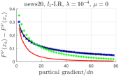
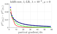
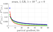
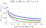
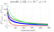
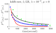
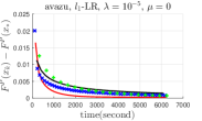
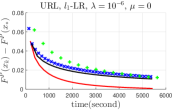
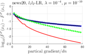
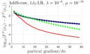
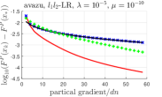
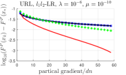
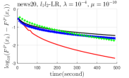
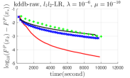
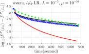
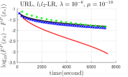
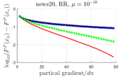
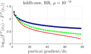
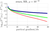
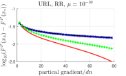
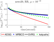
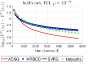
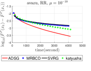
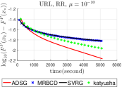
Figure 1: From left to right are the results on news20-binary, kddb-raw, avazu-app, and url-combined.

In this section, we conduct several experiments to show the time efficiency of ADSG on huge-scale real problems.
Problems We conduct experiments of several ERM problems using different regularization functions. For smooth ERM loss, we use logistic regression and least square regression. For non smooth ERM loss, we use SVM and $l_{1}$ regression. We use $\lambda_{1}\cdot\|\cdot\|_{1}$, $\lambda_{2}/2\|\cdot\|_{2}^{2}$, and $\lambda_{1}\cdot\|\cdot\|_{1}+\lambda_{2}/2\cdot\|\cdot\|_{2}^{2}$ for regularization. Four large scale datasets from LibSVM Chang and Lin (2011) are used: kdd2010-raw, avazu-app, new20.binary, and url-combined. Their statistics are given in Table 2.
Algorithms Katyusha  Allen-Zhu (2017), MRBCD Zhao et al. (2014) (ASBCD has similar performance), and SVRG Johnson and Zhang (2013) are included for comparison. MRBCD and ADSG adopts the same block parameter $B$. All methods use the same mini batch size $b$. We use the default inner loop count described in the original paper for SVRG, MRBCD, and Katyusha. We tune the step size to give the best performance. For SVRG and MRBCD, it is usually $1/L$.

6.1 $l_{1}$-Logistic Regression

In this problem, we set $f_{i}(\mathbf{x})=\log(1+\exp(-y_{i}\mathbf{a}_{i}^{\top}\mathbf{x}))$ and set $\mathbf{P}(\mathbf{x})=\lambda\|\mathbf{x}\|_{1}$, where $\{\mathbf{a}_{i},y_{i}\}_{i=1}^{n}$ are data points. We present the accuracy vs. Evaluated Partial Gradients (EPG) and accuracy vs. time in the first two rows of Figure 1, along with the parameter $\lambda$ used in experiments. The result shows that (i) Katyusha and ADSG have superior convergence rate over non-accelerated SVRG and MRBCD, (ii) ADSG and MRBCD, as doubly stochastic methods, enjoy a better time efficiency than Katyusha and SVRG, and (iii) ADSG has the best performance among all competitors.

6.2 $l_{1}l_{2}$-Logistic Regression

$f_{i}(\mathbf{x})$ is $\log(1+\exp(-y_{i}\mathbf{a}_{i}^{\top}\mathbf{x}))$ and $\mathbf{P}(\mathbf{x})$ is $\frac{\mu}{2}\|\mathbf{x}\|^{2}+\lambda\|\mathbf{x}\|_{1}$ in $l_{1}l_{2}$-logistic regression. The accuracy vs. EPG and accuracy vs. time plots are given in the third and fourth rows of Figure 1. We fix $\mu=10^{-10}$ and use the same $\lambda$ in the $l_{1}$-logistic regression. We observe similar phenomenon here as in the previous experiment. Additionally, all methods converge faster in this case, since the problem is strongly convex.

6.3 Ridge Regression

We set $f_{i}(\mathbf{x})=\frac{1}{2}\|\mathbf{a}_{i}^{\top}\mathbf{x}-\mathbf{y}_{i}\|^{2}$ and $\mathbf{P}(\mathbf{x})=\frac{\mu}{2}\|\mathbf{x}\|^{2}$ in this experiment. In the last two rows of Figure 1, we give the accuracy vs. EPG and accuracy vs. time plots. We fix $\mu=10^{-10}$ in all datasets. ADSG shows exceptional computational efficiency in this experiment.

6.4 Solving Non-smooth ERM problem

We conduct experiments on non-smooth ERM problem with linear predictor in this section. Specifically, we assume that $f_{i}(\mathbf{x})=\phi(\langle\mathbf{a}_{i},\mathbf{x}\rangle)$. To use the reduction methods AdaptSmooth and JointAdaptSmoothReg mentioned earlier, we define the auxiliary function

$$\phi^{(\lambda)}(z)=\max_{\beta}z\cdot\beta-\phi^{*}(\beta)-\frac{\lambda}{2}\beta^{2}$$ (19)

where $\phi_{i}^{*}(\beta)=\max_{\alpha}\alpha\beta-\phi_{i}(\alpha)$. We consider two popular problem where $\phi^{(\lambda)}$ admits a closed form.

6.5 Least Absolute Deviation

$f_{i}(\mathbf{x})=\phi_{i}(\langle a_{i},\mathbf{x}\rangle)$, with $\phi_{i}(y)=|y-y_{i}|$. $\phi_{i}^{*}(\beta)=\beta\cdot y_{i}+1_{|\beta|\leq 1}$ and

$$\phi_{i}^{(\lambda)}(\alpha)=\begin{cases}\alpha-y_{i}-\lambda/2,~{}&\alpha>y_{i}+\lambda,\\ (\alpha-y_{i})^{2}/2\lambda,~{}&|\alpha-y_{i}|\leq\lambda,\\ y_{i}-\alpha-\lambda/2,~{}&\alpha<y_{i}-\lambda.\end{cases}$$

Hence we have

$$\partial\phi_{i}^{(\lambda)}(\alpha)=\begin{cases}1,~{}&\alpha>y_{i}+\lambda,\\ (\alpha-y_{i})/\lambda,~{}&|\alpha-y_{i}|\leq\lambda,\\ -1,~{}&\alpha<y_{i}-\lambda.\end{cases}$$

6.6 Support Vector Machine

$f_{i}(\mathbf{x})=\phi_{i}(\langle a_{i},\mathbf{x}\rangle)$, with $\phi_{i}(\alpha)=\max\{0,1-y_{i}\alpha\}$. $\phi_{i}^{*}(\beta)=\beta\cdot y_{i}+1_{-1\leq y_{i}\beta\leq 0}$ and

$$\phi_{i}^{(\lambda)}(\alpha)=\begin{cases}0,~{}&y_{i}\alpha>1,\\ (y_{i}\alpha-1)^{2}/2\lambda,~{}&-\lambda+1\leq y_{i}\alpha\leq 1,\\ 1-y_{i}\alpha-\lambda/2,~{}&y_{i}\alpha<-\lambda+1.\end{cases}$$

Hence we have

$$\partial\phi_{i}^{(\lambda)}(\alpha)=\begin{cases}0,~{}&y_{i}\alpha>1,\\ (\alpha-y_{i})/\lambda,~{}&-\lambda+1\leq y_{i}\alpha\leq 1,\\ -y_{i},~{}&y_{i}\alpha<-\lambda+1.\end{cases}$$

7 Conclusion

An accelerated doubly stochastic algorithm called ADSG is proposed in this paper. We give its convergence analyses, and compare our algorithm to the state-of-the-art in large scale ERM problems. The result is promising.

References

- Allen-Zhu [2017] Zeyuan Allen-Zhu. Katyusha: the first direct acceleration of stochastic gradient methods. In Proceedings of the 49th Annual ACM SIGACT Symposium on Theory of Computing, pages 1200–1205. ACM, 2017.
- Allen-Zhu and Hazan [2016] Zeyuan Allen-Zhu and Elad Hazan. Optimal black-box reductions between optimization objectives. In Advances in Neural Information Processing Systems, pages 1606–1614, 2016.
- Allen-Zhu and Orecchia [2017] Zeyuan Allen-Zhu and Lorenzo Orecchia. Linear Coupling: An Ultimate Unification of Gradient and Mirror Descent. In Proceedings of the 8th Innovations in Theoretical Computer Science, ITCS ’17, 2017. Full version available at http://arxiv.org/abs/1407.1537.
- Beck and Teboulle [2009] Amir Beck and Marc Teboulle. A fast iterative shrinkage-thresholding algorithm for linear inverse problems. SIAM journal on imaging sciences, 2(1):183–202, 2009.
- Chang and Lin [2011] Chih-Chung Chang and Chih-Jen Lin. LIBSVM: A library for support vector machines. ACM Transactions on Intelligent Systems and Technology, 2:27:1–27:27, 2011.
- Defazio et al. [2014] Aaron Defazio, Francis Bach, and Simon Lacoste-Julien. Saga: A fast incremental gradient method with support for non-strongly convex composite objectives. In Advances in Neural Information Processing Systems, pages 1646–1654, 2014.
- Fercoq and Richtárik [2015] Olivier Fercoq and Peter Richtárik. Accelerated, parallel, and proximal coordinate descent. SIAM Journal on Optimization, 25(4):1997–2023, 2015.
- Friedman et al. [2001] Jerome Friedman, Trevor Hastie, and Robert Tibshirani. The elements of statistical learning, volume 1. Springer series in statistics Springer, Berlin, 2001.
- Frostig et al. [2015] Roy Frostig, Rong Ge, Sham M Kakade, and Aaron Sidford. Un-regularizing: approximate proximal point and faster stochastic algorithms for empirical risk minimization. In Proceedings of the 32nd International Conference on Machine Learning (ICML), 2015.
- Hu et al. [2009] Chonghai Hu, Weike Pan, and James T Kwok. Accelerated gradient methods for stochastic optimization and online learning. In Advances in Neural Information Processing Systems, pages 781–789, 2009.
- Johnson and Zhang [2013] Rie Johnson and Tong Zhang. Accelerating stochastic gradient descent using predictive variance reduction. In Advances in Neural Information Processing Systems, pages 315–323, 2013.
- Lan [2012] Guanghui Lan. An optimal method for stochastic composite optimization. Mathematical Programming, 133(1):365–397, 2012.
- Lee and Sidford [2013] Yin Tat Lee and Aaron Sidford. Efficient accelerated coordinate descent methods and faster algorithms for solving linear systems. In Foundations of Computer Science (FOCS), 2013 IEEE 54th Annual Symposium on, pages 147–156. IEEE, 2013.
- Lin et al. [2015a] Hongzhou Lin, Julien Mairal, and Zaid Harchaoui. A universal catalyst for first-order optimization. In Advances in Neural Information Processing Systems, pages 3384–3392, 2015a.
- Lin et al. [2015b] Qihang Lin, Zhaosong Lu, and Lin Xiao. An accelerated randomized proximal coordinate gradient method and its application to regularized empirical risk minimization. SIAM Journal on Optimization, 25(4):2244–2273, 2015b.
- Nesterov [1998] Yu Nesterov. Introductory lectures on convex programming volume i: Basic course. 1998.
- Nesterov [2012] Yu Nesterov. Efficiency of coordinate descent methods on huge-scale optimization problems. SIAM Journal on Optimization, 22(2):341–362, 2012.
- Nesterov [1983] Yurii Nesterov. A method of solving a convex programming problem with convergence rate o (1/k2). In Soviet Mathematics Doklady, volume 27, pages 372–376, 1983.
- Nitanda [2014] Atsushi Nitanda. Stochastic proximal gradient descent with acceleration techniques. In Advances in Neural Information Processing Systems, pages 1574–1582, 2014.
- Polyak [1964] Boris T Polyak. Some methods of speeding up the convergence of iteration methods. USSR Computational Mathematics and Mathematical Physics, 4(5):1–17, 1964.
- Richtárik and Takáč [2014] Peter Richtárik and Martin Takáč. Iteration complexity of randomized block-coordinate descent methods for minimizing a composite function. Mathematical Programming, 144(1-2):1–38, 2014.
- Schmidt et al. [2013] Mark Schmidt, Nicolas Le Roux, and Francis Bach. Minimizing finite sums with the stochastic average gradient. arXiv preprint arXiv:1309.2388, 2013.
- Shalev-Shwartz and Zhang [2013] Shai Shalev-Shwartz and Tong Zhang. Stochastic dual coordinate ascent methods for regularized loss minimization. Journal of Machine Learning Research, 14(Feb):567–599, 2013.
- Shalev-Shwartz and Zhang [2014] Shai Shalev-Shwartz and Tong Zhang. Accelerated proximal stochastic dual coordinate ascent for regularized loss minimization. In ICML, pages 64–72, 2014.
- Simon et al. [2013] Noah Simon, Jerome Friedman, Trevor Hastie, and Robert Tibshirani. A sparse-group lasso. Journal of Computational and Graphical Statistics, 22(2):231–245, 2013.
- Tibshirani [1996] Robert Tibshirani. Regression shrinkage and selection via the lasso. Journal of the Royal Statistical Society. Series B (Methodological), pages 267–288, 1996.
- Woodworth and Srebro [2016] Blake E Woodworth and Nati Srebro. Tight complexity bounds for optimizing composite objectives. In Advances in Neural Information Processing Systems, pages 3639–3647, 2016.
- Wright [2015] Stephen J Wright. Coordinate descent algorithms. Mathematical Programming, 151(1):3–34, 2015.
- Zhang and Gu [2016] Aston Zhang and Quanquan Gu. Accelerated stochastic block coordinate descent with optimal sampling. In Proceedings of the 22nd ACM SIGKDD International Conference on Knowledge Discovery and Data Mining, pages 2035–2044. ACM, 2016.
- Zhang and Xiao [2015] Yuchen Zhang and Lin Xiao. Stochastic primal-dual coordinate method for regularized empirical risk minimization. In Proceedings of the 32nd International Conference on Machine Learning, volume 951, page 2015, 2015.
- Zhao et al. [2014] Tuo Zhao, Mo Yu, Yiming Wang, Raman Arora, and Han Liu. Accelerated mini-batch randomized block coordinate descent method. In Advances in neural information processing systems, pages 3329–3337, 2014.