Reconstruction of an Observationally Constrained gravity model
Anirudh Pradhan1, Gopikant Goswami2, Aroonkumar Beesham3,4
1Centre for Cosmology, Astrophysics and Space Science (CCASS), GLA University, Mathura-281 406, Uttar Pradesh, India
2Department of Mathematics, Netaji Subhas University of Technology, Delhi, India
3Department of Mathematical Sciences, University of Zululand Private Bag X1001 Kwa-Dlangezwa 3886 South Africa
4Faculty of Natural Sciences, Mangosuthu University of Technology, P O Box 12363, Jacobs 4052, South Africa
1E-mail: pradhan.anirudh@gmail.com
2E-mail: gk.goswami9@gmail.com
3,4E-mail: abeesham@yahoo.com
Abstract
In this paper, an attempt is made to construct a Friedmann-Lemaitre-Robertson-Walker model in gravity with a perfect fluid that yields acceleration at late times. We take as + . As in the CDM model, we take the matter to consist of two components, viz., and such that + =1. The parameter is the matter density (baryons + dark matter), and is the density associated with the Ricci scalar and the trace of the energy momentum tensor, which we shall call dominant matter. We find that at present is dominant over , and that the two are in the ratio 3:1 to 3:2 according to the three data sets: (i) 77 Hubble OHD data set (ii) 580 SNIa supernova distance modulus data set and (iii) 66 pantheon SNIa data which include high red shift data in the range . We have also calculated the pressures and densities associated with the two matter densities, viz., , , and , respectively. It is also found that at present, is greater than . The negative dominant matter pressure creates acceleration in the universe. Our deceleration and snap parameters show a change from negative to positive, whereas the jerk parameter is always positive. This means that the universe is at present accelerating and in the past it was decelerating. State finder diagnostics indicate that our model is at present a dark energy quintessence model. The various other physical and geometric properties of the model are also discussed.
Keywords: theory; FLRW metric; Observational parameters; Transit universe; Observational constraints
Mathematics Subject Classification 2020: 83D05, 83F05, 83C15
1 Introduction:
Cosmology is the study of the large scale structure and evolution of the universe. It began seriously with the simple Einstein static universe [1]. It then got a drastic change due to Hubble [2], who started the concept of an expanding universe. This was later mathematically formulated into the FLRW (Friedmann-Lemaitre-Robertson-Walker) spacetime [3, 4, 5, 6, 7]. The universe since its inception, passed through very exotic events such as inflation [8, 9] at the beginning, then the discovery of the CMB (cosmic microwave background radiation) [10], and then the late time acceleration[11][26]. Dark energy, which is believed to cause this acceleration is most often represented by the very simple concordance CDM model. This model fits well on observational grounds [27][29], despite certain weaknesses [30] that it suffers with fine tuning and the cosmic coincidence problems. To solve these, scalar field dominated tracker field quintessence and phantom dark energy models were proposed [31][34]. Later on, parameterizations for the scalar field were suggested, and some interesting cosmological models were developed [35] [42]. This work has been done under the principle of general relativity (GR) and accordingly, the GR field equations were used.
With this, a spate of work was begun in which attempts were made to get an accelerating universe by modifying Einstein’s field equations. It has been suggested that the Ricci scalar be replaced by an arbitrary function of in the Einstein-Hilbert action, and that the new theory and its field equations be called theory [43] [56]. The idea is that a non linear Ricci scalar may be helpful in developing negative pressure in the universe, producing acceleration. Seeing the complexity of solutions due to non linear Ricci scalar [57], more alternatives were proposed. In one of the options, was replaced by an arbitrary function of and where is the trace of the energy momentum tensor. This theory is called gravity [58] [71]. The authors of the theory [58] have dealt three options for the specific functional form of ), especially for cosmological interpretations. They are .
The purpose of this work is to model a universe in gravity which meets observational constraints [20][22].
For this, we consider the first simple alternative of , i.e., T, taking as an arbitrary constant. We consider an FLRW spacetime with perfect fluid. Our three model parameters, viz., the Hubble, deceleration and equation of state, are estimated with the help of three data sets: (i) the 77 Hubble OHD data set [72][87] (ii) the 580 SNIa supernova distance modulus data set [17] and (iii) the 66 pantheon SNIa data set, which includes the high red shift data in the range [88][90]. We solve the field equations by making the simplest possible parametrization of the equation of state parameter as given by Gong and Zhang [35].
At this junction, it is desirable to describe the new results/important points presented in this paper which are different from the past studies. In the past there had been some very interesting reconstruction and review works in the modified theories of gravity [69] [73]. The learned authors also noticed certain finite time singularities and rips in certain models. However as an important and noticeable feature in our model, we have developed two energy parameters and and found that + =1. The parameter is associated with the matter, whereas is associated with gravity. We have statistically estimated using high red shift data set in the range that at present is dominant, and that the two energy densities are approximately in the ratio 3:1 to 3:2. Moreover we have also performed a state finder diagnostic of our model and found that our model is at present in quintessence. We have presented 35 plots and tables to describe the findings of our work more effectively.
The following is a short description of the work, broken down into sections: In section , the field equation for a perfect fluid filled FLRW space time are described. Section is the architect of the rest of the part of the paper. In this section, we get expressions for the Hubble and deceleration parameters as functions of red shift. In sections , and , the model parameters have been estimated on the basis of the three data sets. In sections 7, we have presented the error bar plots, confidence regions and likelihood plots for the Hubble, distance modulus and apparent magnitude. The purpose here is to show the proximity of observational and theoretical results. The jerk and snap parameters are discussed in section 8, and it is found that our model is at present a dark energy quintessence model. In section , we have obtained expressions for the densities and pressures. It is found that at present density () is dominant over baryon density and they are nearly in the ratio 1:3 or 2:3 as per different observed data sets. The last section is devoted to the concluding remarks.
2 f(R,T) Field Equations for Perfect Fluid Filled FLRW Space Time:
We refer to [58] for the field equations of f(R,T) gravity:
| (1) |
where we take the energy momentum tensor as that of perfect fluid:
| (2) |
The other symbols in the field equations (1) have their usual meanings. The Einstein Hilbert action is:
| (3) |
where is the matter Lagrangian. The field equations (1) are obtained replacing the Ricci scalar R by a arbitrary function of and trace of energy momentum tensor . Accordingly, the action is:
| (4) |
The FLRW metric is:
| (5) |
We solve Eqs. (1) and (2) for this metric and get:
| (6) |
and
| (7) |
where is the Hubble parameter.
3 Deceleration and Hubble Parameters:
| (8) |
and
| (9) |
where is deceleration parameter and . It is clear from the field equations (8) and (9) that for , these equations reduce to those of general relativity. So the additional terms containing are there due to gravity. We require (acceleration) at present due to the presence of these terms. We let:
| (10) |
and call these the dominant pressure and dominant energy density, respectively, for reasons which will become clear later. These may be regarded as the contribution of gravity to the pressure and density. We get the energy parameters and and the equations of state parameter and as follows:
| (11) |
Here suffixes and stands for the GR effect, and effect, respectively. We may also interpret the parameters with the suffix as terms arising due to the curvature dominance of gravity.
From Eqs. (8) (11), we get the following:
| (12) |
and
| (13) |
Eqs. (12) and (13) give us the following expression for :
| (14) |
From this, we get the present value of as:
| (15) |
We observe that there are two equations and four unknowns , , and . Hence, one cannot solve these equation in general. However, to get an explicit solution of the above equations, we have to assume at least one reasonable relation among the variables. For this, we consider the simplest parametrization of the equation of state parameter as given by Gong and Zhang [35]:
| (16) |
where is the red shift and is the present value of the equation of state parameter . With this we can now solve for in term of as follows:
| (17) |
Then H may be obtained from q by solving the following differential equation:
| (18) |
We obtain the expression for as follows:
| (19) |
where, is the present value of the Hubble parameter and:
4 Estimation of , and from A Observed Hubble Data Set:
In this section we will estimate the present values of , and statistically from a data set of observed values of H at different red shifts using (a) The cosmic chronometric method, (b) the BAO signal in galaxy distribution and (c) the BAO signal in the Ly forest distribution alone or cross-correlated with QSOs [72][87]. We compare the data set values from those obtained theoretically from Eq. (19) by forming the following chi square function of , and .
| (20) |
These parameters are estimated by getting the minimum value of chi squared for the values of the parameters taken in the range ( ,6575), (, -0.60 -0.40) and (, -0.90 -0.70) . It is found that
for minimum chi squire =0.685263 which is a a good fit. The fit will be more clear from the following error bar and livelihood plots in figure .
Figures and describe the growth of and over red shift , respectively. H is an increasing function of z. These figures also show the closeness of the theoretical graph to the observed values. Figures , and are likelihood probability curves for , and . Estimated values on the basis of the 77 OHD data set are .
(a) 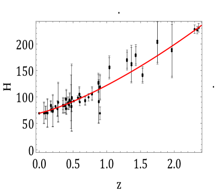 (b)
(b) 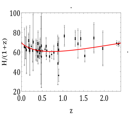 (c)
(c) 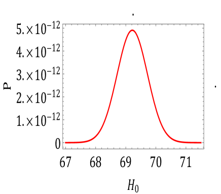 (d)
(d) 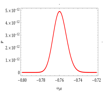
(e) 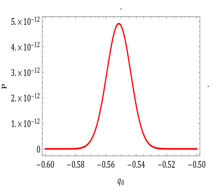
Figures , , and are the 1, 2 and 3 confidence region plots for the pair of parameters (, ), (, ) and (, ). The estimated value points , and are red spotted. These are just there to show that our estimated values are within the statistically specified regions.
(a) 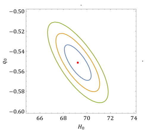 (b)
(b) 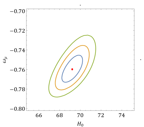 (c)
(c) 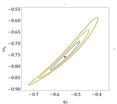
5 Distance Modulus and Apparent Magnitude for the Model:
The luminosity distance () plays a very important parameter for observing distances of luminous objects like standard kindles, population I and II stars. The luminosity distance of the SN Ia supernovae was found to be more than expected, which has given rise to the concept of the accelerating universe [11, 12]. is given by:
| (21) |
where, and are the absolute and apparent magnitudes, respectively. is called distance modulus. and are defined by
| (22) |
and
| (23) |
As we have already obtained expressions for H, we can determine and We can also obtain expressions for apparent magnitude from these expressions. For this we use two important observations (i.) The absolute magnitude of all standard candles are assumed to be the same, and (ii) The luminosity distance of very low red shift SNIa are approximated as Using these facts and taking a low red shift supernova with red shift and , we find With this, we obtain the expression for the apparent magnitude as follows:
| (24) |
6 Estimation of Model parameters from distance modulus and apparent data sets:
We use two standard data sets (i) 580 SN Ia data set of distance modulus (DM) in the red shift range (ii) 66 pantheon data set of SN Ia apparent magnitude (AP) comprising 40 bin plus 16 high red shift data in the range . We consider theoretical results of distance modulus and apparent magnitude as obtained from Eqs. (21) and (24), as function of model parameters , and . In these expressions we take red shifts from the data sets. Thus we form a parallel data set of theoretical results. With these, we form two chi squire functions separately for the DM and AP as follows:
| (25) |
and
| (26) |
If the parameters and be given in the range ( , 6575), (, -0.60 -0.40) and (, -0.90 -0.70), we find for the data set, , whereas for AP data set it is More over if we combine Hubble 77 data set and 580 distant modulus data set make a pool of 657 data set we get the following result: We present the following table to display all of our statistical findings:
| Datasets | ||||
|---|---|---|---|---|
| 77 H | -0.759826 | 52.0805 | ||
| 580 D.M | -0.804005 | 562.245 | ||
| 66 A.M | -0.798498 | 71.861214 | ||
| 657 H + D.M | -0.806833 | 615.311 |
Figure describes the growth of distant modulus over red shift . The distant modulus is increasing function of red shift which means that in the past distant modulus was more. It is gradually decreasing over time. The figure also shows that theoretical graph passes near by through the 580 vertical error lines whose middle points are observed values at different red shifts. Figure , and are the 1, 2 and 3 confidence region plots for the pair of parameters (, ), (, ) and (, ). The estimated value points , and are red spotted. These are just there to show that our estimated values are within the statistically specified regions.
(a) 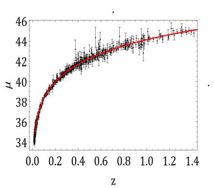 (b)
(b) 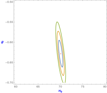 (c)
(c) 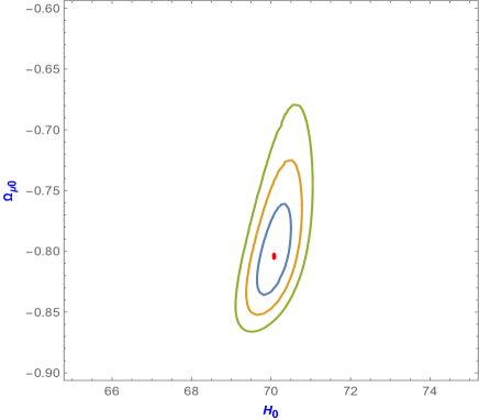 (d)
(d) 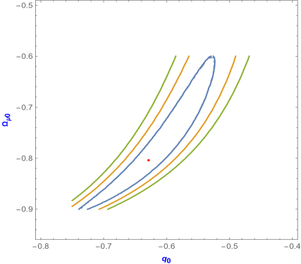
Figures , and are likelihood probability curves for Hubble , deceleration and equation of state parameters. Estimated values on the basis of 580 SNIa D.M.() data set are at the peak.
(a) 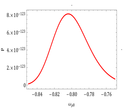 (b)
(b)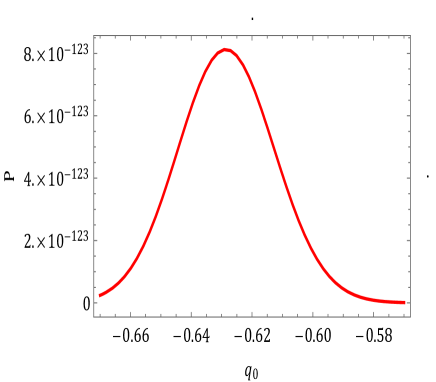 (c)
(c)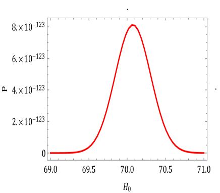
Figure describes the growth of AM over red shift . The AM is increasing function of red shift which means that in the past DM was more. It is gradually decreasing over time. The figure also shows that theoretical graph passes near by through the 66 vertical error lines whose middle points are observed values of AP at different red shifts. Figure are the 1, 2 and 3 confidence region plots for the pair of parameters (, ), (, ) and (, ). The estimated value points , and are red spotted.
(a) 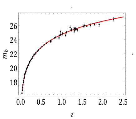 (b)
(b)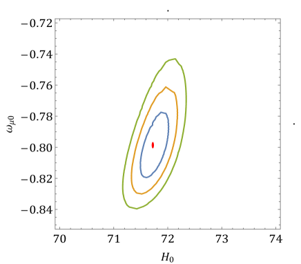 (c)
(c) (d)
(d) 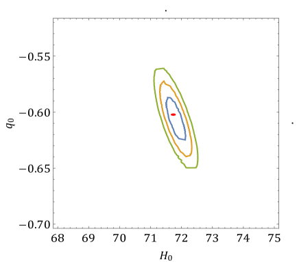
Figures , and are likelihood probability curves for Hubble , deceleration and equation of state parameters. Estimated values on the basis of 66 Pantheon apparent modulus data set are at the peak.
(a)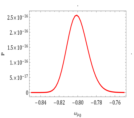 (b)
(b) (c)
(c) 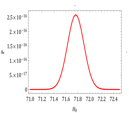
6.1 Determination of the present values of Energy parameters and :
In sections and , we have estimated the present values of , , and on the basis of four data sets which are described in Table-1. From Eqs. (13) and (14), we obtain values of and for matter. From Eq. (9), we get energy parameters and as follows:
| (27) |
| Datasets | ||||
|---|---|---|---|---|
| 77 H | 0.311089 | 0.688911 | ||
| 580 D.M | 0.320414 | 0.679586 | ||
| 66 A.M | 0.386145 | 0.613855 | ||
| 657 H + D.M | 0.39028 | 0.60972 |
In this table, we find that at present is dominant and it is nearly in the ratio 1:3 or 2:3 as per different observed data sets. We note that is due to the curvature and energy momentum dominance in gravity.
7 Plots of Deceleration, Jerk and Snap Parameters:
The jerk (j) and snap (s) parameters are related to the third and fourth order derivatives of the scale factor. They play a very important role in examining the instability of a cosmological model. The jerk also plays a role in statefinder diagnostics. They are defined as: and j in the terms of q can be written as:
| (28) |
whereas s in terms of q and j is computed as:
| (29) |
Having estimated the present values of , , and in sections and , we can plot and analyse q, j and s which are presented in the following figures.
(a)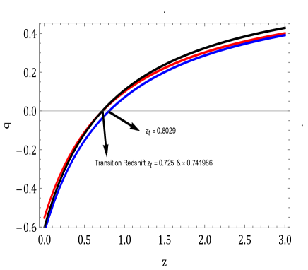 (b)
(b)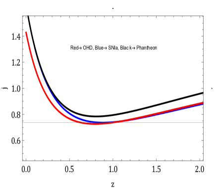 (c)
(c) 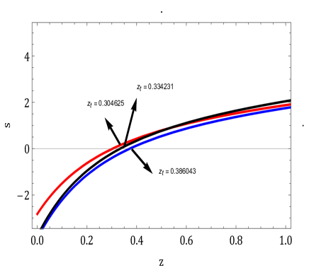
We make following observations from the three plots of Figure
-
•
q and s show a transition from negative to positive, which indicates that the universe is accelerating at present, and it was decelerating in the past.
-
•
The Transition red shifts are well within the observational results
-
•
j is always positive. Its present values are 1.42783, 1.6416 and 1.64327 as per the OHD, SNIa and pantheon data sets. These values are greater than one, which shows that this model behaves differently from the CDM concordance model where j=1.
8 Statefinder Diagnostic:
In this important section, we use a very useful diagnostic technique given by Sahni et al. [41]. They have used a pair of statefinder parameters depending on the scale factor . The purpose is to differentiate cosmological models from the standard CDM concordance model. The techniques also describe the evolution of the models in the sense that it indicates through which phases the model has passed through. is defined as follows:
| (30) |
where is the jerk parameter.
We plot two parametric curves, one with against , and the other with against .
(a)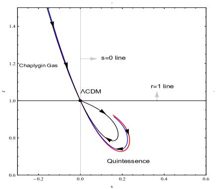 (b)
(b)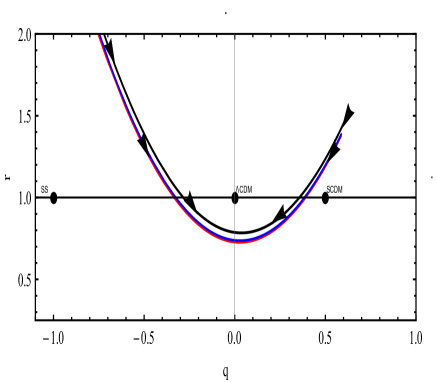
We make following observations as reflected in the two plots of Figure :
-
•
Fig (a) shows that the three parametric (s,r) curves based on the the estimated values of the OHD, SNIa and phantom data sets meet at CDM point(1,0) from both directions, i.e., from the Chaplygin gas model to quintessence.
-
•
At present, our model is in quintessence.
-
•
The Fig. (b) also tells us that our model does not approximate the CDM model, nor was it the Einstein-Desitter model in the past.
9 Density and Pressure in the Model:
| (31) |
| (32) |
and
| (33) |
We can express the density and pressure in a more convenient way as follows:
| (34) |
| (35) |
where is the critical density and it has the value , h=. The other parameters like , , and have been estimated by us. So we can plot the matter density and pressure. From Eqs. (34), (32) and (10), we can plot and . We note that these develop due to the curvature and trace of the energy momentum tensor dominance in gravity. The followings are the plots:
(a) 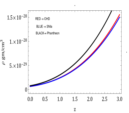 (b)
(b)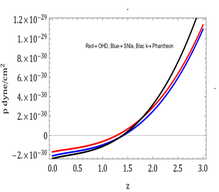 (c)
(c)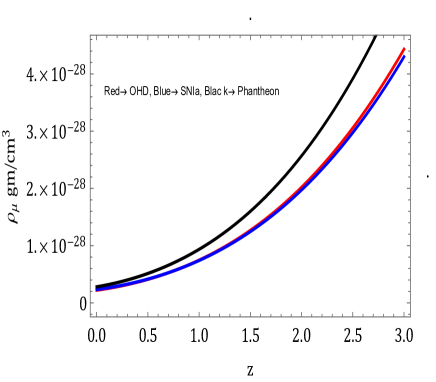 (d)
(d) 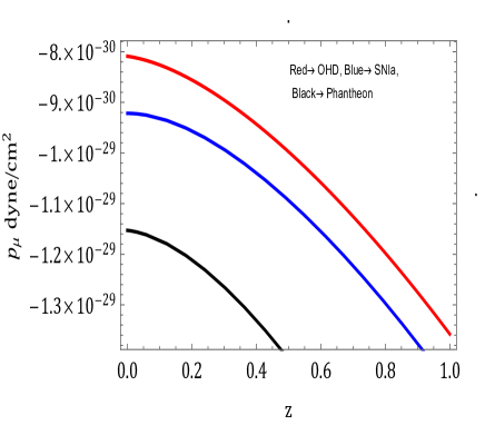
We make following observations from these the four plots of the Figure .
-
•
We can compare the matter and densities in the following way:
At present the ratio of the two densities is obtained from Table-1 as as per the OHD, SNIa and Pantheon data sets, respectively. This shows that quantitatively, the density is more than the matter density.
-
•
The matter pressure is very small, i.e., dust.
-
•
The pressure is negative. This is responsible for the present day acceleration in the universe.
-
•
Both matter density and pressure are increasing functions of red shift.
-
•
The density is also showing the same trend as that of the matter.
9.1 Effective density and Effective pressure:
Equation (12) may be written as
| (36) |
where and We can express these in a more convenient way as follows:
| (37) |
(a) 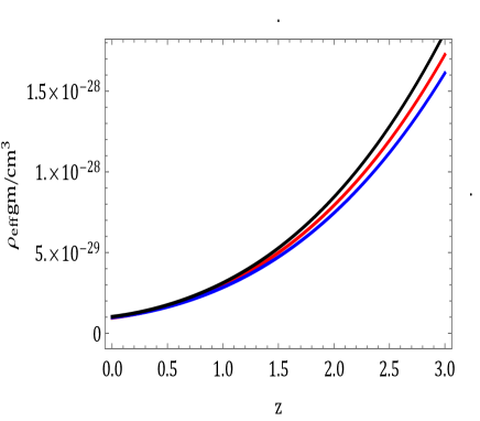 (b)
(b)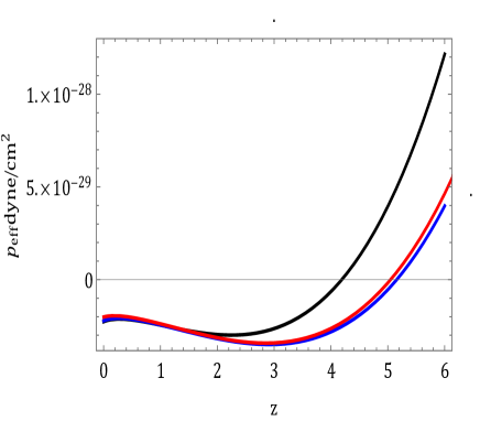 (c)
(c)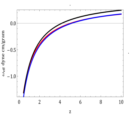
We make following observations from these the three plots of the Figure :
-
•
The density is increasing decreasing with time. The present value of is equal to the critical density.
-
•
Both pressure and equation of state parameter are showing a change from negative to positive, showing that our universe is accelerating, and in the past it was decelerating.
9.2 Time versus Red Shift and Transitional times:
We can calculate the time of any event from the red shift through the following transformation
| (38) |
where is the present time and some past time, respectively. We note that at present, t= and z=0. With the help of expression for the Hubble parameter Eq. (18), we can plot the graph of time versus red shift. This is given in the following figure .
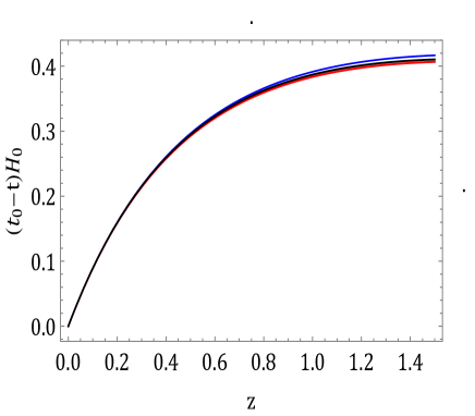
We make the following observations from the plot of the Figure :
-
•
The three plots are based on the estimations of the model parameters for the three data sets (i) OHD (ii) SNIa and (iii) pantheon, and they are almost identical.
-
•
As yrs, where , we can calculate the transition time for the deceleration parameter, and they are , . These correspond to the transition red shifts .
10 Conclusion:
We can summarise our finds as follows:
-
•
We attempted to model an FLRW model filled with a perfect fluid in gravity, where is taken as + T.
-
•
We developed two energy parameters and and used the relation that + =1. The parameter is associated with the matter, whereas is associated with gravity. We have statistically estimated that at present is dominant, and that the two energy densities are approximately in the ratio 3:1 to 3:2.
-
•
We have also introduced pressure () and density () along with the matter pressure and density. We find that at present the density () is dominant over the matter density and they are nearly in the ratio 1:3 to 2:3. The negative pressure () is associated with the acceleration in the universe.
-
•
Our model parameters are the present values of the Hubble, deceleration and equation of state parameters. These parameters were estimated with the help of the three data sets: (i) 77 Hubble OHD data set (ii) 580 SNIa supernova distance modulus data set and (iii) 66 pantheon SNIa which include high red shift data in the range .
-
•
Our deceleration and snap parameters show transition from negative to positive and the jerk is always positive. . We have performed a state finder diagnostic of our model and found that our model is at present in quintessence.
-
•
All of our findings are displayed in Table-1 and Table-2. The results are well within the observational findings.
-
•
All of our outcomes are expressed in terms of red shifts and we have presented transformation to convert red shift into time. Accordingly we have obtained transition times for our deceleration parameter. From the cosmological analyses, we infer that modifying Einstein’s field equations by replacing Ricci scalar by an arbitrary function of ans trace of energy momentum tensor in the Einstein-Hilbert action may lead to arrive at a model which describe transition from deceleration to acceleration at late time. This can be seen as a one step more ahead of the fundamental theory of general relativity physics on gravitation.
Acknowledgments
The authors (A. Pradhan & G.K. Goswami ) are grateful for the assistance and facilities provided by the University of Zululand, South Africa during a visit where a part of this article was completed.
References
- [1] C. O’Raifeartaigh, M. O’Keeffe, W. Nahm and S. Mitton, Einstein’s 1917 static model of the universe: a centennial review, Eur. Phys. J. H. 42 (3) (2017) 431–474.
- [2] E. Hubble, A relation between distance and radial velocity among extra-galactic nebulae, Proceed, Nat. Acad. Scien. 15 (3) (1929) 168–173.
- [3] A. Friedman, ber die Krmmung des Raumes, Zeitschrift für Physik. 10 (1) (1922) 377-386.
- [4] G. Lemaitre, Expansion of the universe, A homogeneous universe of constant mass and increasing radius accounting for the radial velocity of extra-galactic nebulae, Month. Not. Roy. Astron. Soci. 91 (5) (1931) 483-490.
- [5] H. P. Robertson, Kinematics and world structure, Astrophys. J. 82 ( 1935) 284-301.
- [6] H. P. Robertson, Kinematics and world structure III, Astrophys. J. 83 (1936) 257-271.
- [7] A. G. Walker, On Milne’s theory of world-structure, Proceed. London Math. Soci. Series 2 42 (1) (1937) 90-127.
- [8] S. Tsujikawa, Introductory review of cosmic inflation, arXiv:hep-ph/0304257 ( 2003)
- [9] J. Earman and J. Mosterin, A Critical Look at Inflationary Cosmology, Philosophy of Science 66 (1) (1999) 1-49.
- [10] A. A. Penzias and R. W. Wilson, A measurement of excess antenna temperature at 4080 Mc/s, The Astrophys. J. 142 (1) (1965) 419-421.
- [11] A. G. Riess, et al. [Supernova Search Team], Observational evidence from supernovae for an accelerating universe and a cosmological constant, Astron. J. 116 (1998) 1009-1038.
- [12] S. Perlmutter, et al. [Supernova Cosmology Project], Measurements of and from 42 high redshift supernovae, Astrophys. J. 517 (1999) 565-586.
- [13] J. L. Tonry, et al., Cosmological results from high-z supernovae, Astrophys. J. 594 (2003) 1.
- [14] A. Clocchiatti, et al., Hubble Space Telescope and ground-based observations of type Ia Supernovae at redshift 0:5: cosmological implications, Astrophys. J. 642 (2006) 1.
- [15] D. N. Spergel, et al. [WMAP collaboration], First year wilkinson microwave anisotropy probe (WMAP) observations determination of cosmological parameters, Astrophys. J. Suppl. 148 (2003) 175.
- [16] M. Tegmark, et al. [SDSS collaboration], Cosmological parameters from SDSS and WMAP, Phys. Rev. D 69 (2004) 103501.
- [17] N. Suzuki, et al., The Hubble space telescope cluster supernova survey V improving the darkenergy constraints above z 1 and building an early-type-hosted supernova sample, Astrophys. J. 746 (2012) 85-115.
- [18] T. Delubac, et al. [BOSS Collaboration], 2015. Baryon acoustic oscillations in the Ly forest of BOSS DR11 quasars, Astron. Astrophys. 574 (2015) A59.
- [19] C. Blake, et al. [The Wiggle Z Dark Energy Survey], 2012. The Wiggle Z dark energy survey joint measurements of the expansion and growth history at , Mon. Not. R. Astron. Soc. 425 (2012) 405-414.
- [20] P. A. R. Ade, et al. [Planck Collaboration], 2016. Planck 2015 results XIV dark energy and modied gravity, Astron. Astrophys. 594 (2016) A14.
- [21] E. Komatsu, et al., Seven-Year Wilkinson Microwave Anisotropy Probe (WMAP) Observations: Cosmological interpretation, Astrophys. J. Suppl. 192 (2011) 18.
- [22] N. Aghanim et al., Planck 2018 results. VI. Cosmological parameters, Astron. Astrophys. 641 (2020) A6. [erratum: Astron. Astrophys. 652 (2021) C4.
- [23] S. Alam et al. (BOSS Collaboration), The clustering of galaxies in the completed SDSS-III Baryon Oscillation Spectroscopic Survey: cosmological analysis of the DR12 galaxy sample, Mon. Not. Roy. Astron. Soc. 470 (2017) 2617-2652.
- [24] O. H. E. Philcox, M. M. Ivanov, M. Simonovic, and M. Zaldarriaga, Combining full-shape and BAO analyses of galaxy power spectra: A 1.6% CMB-independent constraint on H0, JCAP 2020(05) (2020) 032.
- [25] O. H. E. Philcox, B. D. Sherwin, G. S. Farren, and E. J. Baxter, Determining the Hubble constant without the sound horizon: Measurements from galaxy surveys, Phys. Rev. D 103 (2021) 023538.
- [26] T. Colas, G. D’amico, L. Senatore, P. Zhang, and F. Beutler, Efficient cosmological analysis of the SDSS/BOSS data from the effective field theory of large-scale structure, JCAP 2020(06) (2020) 001.
- [27] E. J. Copeland, M. Sami, and S. Tsujikawa, Dynamics of dark energy, Int. J. Mod. Phys. D 15 (2006) 1753-1936.
- [28] M. Li, X.-D. Li, S. Wang, and Y. Wang, Dark energy, Commun. Theor. Phys. 56 (2011) 525-604.
- [29] O. Gron and S. Hervik, Einstein’s general theory of relativity with modern applications in cosmology (Springer Publication, 2007).
- [30] S. Weinberg, The cosmological constant problem, Rev. Mod. Phys. 61 (1989) 1.
- [31] P. J. E. Peebles and B. Ratra, The Cosmological constant and dark energy, Rev. Mod. Phys. 75 (2003) 559-606.
- [32] V. B. Johri, Genesis of cosmological tracker fields, Phys. Rev. D 63 (2001) 103504.
- [33] R. R. Caldwell, A phantom menace? Cosmological consequences of a dark energy component with super-negative equation of state, Phys. Lett. B 545 (2002) 23-29.
- [34] V. B. Johri, Phantom cosmologies, Phys. Rev. D 70 (2004) 041303
- [35] Y. Gong and Y. Zhang, Probing the curvature and dark energy, Phys. Rev. D 72 (2005) 043518.
- [36] D. Huterer and M. S. Turner, Probing dark energy: Methods and strategies, Phys. Rev. D 64 (2001) 123527.
- [37] E. V. Linder, Exploring the expansion history of the universe, Phys. Rev. Lett. 90 (2003) 91301.
- [38] T. Roy Choudhary and T. Padmanabhan, Cosmological parameters from supernova observations: A critical comparison of three data sets, Astron. & Astrophys. 429 (2005) 807-818.
- [39] B. Feng, X. Wang, and X. Zhang, Dark energy constraints from the cosmic age and supernova, Phys. Lett. B 607 (2005) 35-41.
- [40] S. Lee, Constraints on the dark energy equation of state from the separation of CMB peaks and the evolution of , Phys. Rev. D 71 (2005) 123528.
- [41] H. K. Jassal, J. S. Bagla, and T. Padmanabhan, WMAP constraints on low redshift evolution of dark energy, Mon. Not. Roy. Astron. Soci.: Lett. 356 (2005) L11-L16.
- [42] T. Padmanabhan and T. Roy Choudhury, A theoretician’s analysis of the supernova data and the limitations in determining the nature of dark energy, Mon. Not. Roy. Astron. Soci.: Lett. 344 (2003) 823-834.
- [43] H. Motohashi, A. A. Starobinsky, and J. Yokoyama, gravity and its cosmological implications, Int. J. Mod. Phys. D 20 (2011) 1347-1355.
- [44] S. Nojiri and S. D. Odintsov, Introduction to modified gravity and gravitational alternative for dark energy, Int. J. Geomet. Methods Mod. Phys. 4.01, (2007) 115-145.
- [45] T. P. Sotiriou and V. Faraoni, theories of gravity, Rev. Mod. Phys. 82, (2010) 451-497.
- [46] F. S. N. Lobo, The Dark side of gravity: Modified theories of gravity, arXiv:0807.1640 [gr-qc] (2008).
- [47] S. Capozziello and M. Francaviglia, Extended theories of gravity and their cosmological and astrophysical applications, Gen. Rel. Grav. 40 (2008) 357-420; S. Camera, S. Capozziello, L. Fatibene and A. Orizzonte, The effective Equation of State in Palatini f(R) cosmology, arXiv:2212.13825 [gr-qc]; F. Bajardi, R. D’Agostino, M. Benetti, V. De Falco and S. Capozziello, Early and late time cosmology: the f (R) gravity perspective, Eur. Phys. J. Plus 137 (2022) 1239; H. Abedi, S. Capozziello, M. Capriolo and A. M. Abbassi, Gravitational energy–momentum pseudo-tensor in Palatini and metric f (R) gravity, Annals Phys. 439 (2022) 168796; A. V. Astashenok, S. Capozziello, S. D. Odintsov and V. K. Oikonomou, Maximum baryon masses for static neutron stars in f (R) gravity, Europhys. Lett. 136 (2022) 59001; G. G. L. Nashed and S. Capozziello, Anisotropic compact stars in f(R) gravity, Europ. Phys. J. C 81 (2021) 481.
- [48] S. Nojiri, S. D. Odintsov, and O. G. Gorbunova, Dark energy problem: from phantom theory to modified Gauss-Bonnet gravity, Journal of Physics A: Mathematical General, 39 (2006) 6627.
- [49] A. Chudaykin, K. Dolgikh, and M. M. Ivanov, Constraints on the curvature of the universe and dynamical dark energy from the full-shape and BAO data, Phys. Rev. D 103 (2021) 023507.
- [50] S. Nojiri and S. D. Odintsov, Modified gravity with negative and positive powers of the curvature: Unification of the inflation and of the cosmic acceleration, Phys. Rev. D 68 (2003) 123512.
- [51] A. A. Starobinsky, Disappearing cosmological constant in gravity, JETP Lett. 86 (2007) 157-163.
- [52] T. P. Sotiriou and S. Liberati, Metric-affine theories of gravity, Annals Phys. 322 935-966 (2007).
- [53] S. K. Srivastava, Early and Late Transient Cosmic Acceleration due to Curvature Inspired Dark Energy, Phys. Lett. B 648 (2007) 119-126.
- [54] A. Mukherjee and N. Banerjee, Acceleration of the Universe in Gravity Models, Astrophys. Space Sci. 352 (2014) 893-898.
- [55] G. C. Samanta and N. Godani, Physical Parameters for Stable Models, Indian J. Phys. 94 (2019) 1303-1310.
- [56] G. K. Goswami, R. Rani, H. Balhara, and J. K. Singh, Curvature dominance DE-model in -gravity arXiv preprint arXiv:2204.07604 (2022).
- [57] L. Amendola and S. Tsujikawa, Dark Energy: Theory and Observations (Cambridge University Press, Cambridge, 2013).
- [58] T. Harko, F. S. N. Lobo, S. Nojiri, and S. D. Odintsov, gravity, Phys. Rev. D 84 (2011) 024020.
- [59] R. Chaubey and A. K. Shukla, A new class of Bianchi cosmological models in gravity, Astrophys. Space Sci. 343 (2013) 415.
- [60] S. B. Fisher and E.D. Carlson, Reexamining gravity, Phys. Rev. D 100 (2019) 064059.
- [61] T. Harko and P. H. R. S. Moraes, Comment on Reexamining gravity, Phys. Rev. D 101 (2020) 108501.
- [62] G. A. Carvalho, R. V. Lobato, P. H. R. S. Moraes, J. D. V. Arbail, R. M. Marinho, J. E. Otoniel, and M. Malheiro, Stellar equilibrium configurations of white dwarfs in the gravity, Eur. Phys. J. C 99 (2017) 871.
- [63] A. K. Yadav, P. K. Sahoo, and V. Bhardwaj, Bulk viscus Bianchi-I embedded cosmological model in gravity, Mod. Phys. Lett. A 34, (2019) 1950145.
- [64] L. K. Sharma, B. K. Singh, and A. K. Yadav, Viability of Bianchi type universe in gravity, Int. J. Geom. Methods Mod. Phys. 17 (2020) 2050111.
- [65] L. K. Sharma, A. K. Yadav, P. K. Sahoo, and B. K. Singh, Non-minimal matter-geometry coupling in Bianchi I space-time, Results Phys. 10 (2018) 738.
- [66] V. K. Bhardwaj and A. Pradhan, Evaluation of cosmological models in gravity in different dark energy scenario, New Astronomy 91 (2022) 101675.
- [67] T. Tangphati, S. Hansraj, A. Banerjee, and A. Pradhan, Quark stars in f(R, T) gravity with an interacting quark equation of state, Phys. Dark Univ. 35 (2022) 100990.
- [68] J. M. Z. Pretel, T. Tangphati, A. Banerjee, and A. Pradhan, Charged quark stars in gravity, Chin. Phys. C 46 (2022) 115103; V. K. Bhardwaj, A. Pradhan, N. Ahmed and A. A. Shaker, Cosmographic analysis of a closed bouncing universe with the varying cosmological constant in f(R, T) gravity, Can. J. Phys. 100 (2022) 475-484; A. Pradhan, A. Dixit and G. Varshney, LRS Bianchi type-I cosmological models with periodic time varying deceleration parameter and statefinder in gravity, Int. J. Mod. Phys. A 37 (2022) 2250121; V. K. Bhardwaj and A. Pradhan, Evaluation of cosmological models in gravity in different dark energy scenario, New Astronomy 91 (2022) 101675; A. Dixit, P. Garg and A. Pradhan, FRW cosmological models with cosmological constant in theory of gravity, Can. J. Phys. 199 (2021) 741-753; C. Chawla, A. Dixit and A. Pradhan, Modeling of traversable wormholes in exponential f(R, T) gravity, Can. J. Phys. 199 (2021) 634-645; R. K. Tiwari, A. Beesham and A. Pradhan, Transit cosmological models with domain walls in gravity, Gravit. & Cosmol. 23 (2017) 392-400.
- [69] K. Bamba, S. Capozziello, S. Nojiri and S. D. Odintsov, Dark energy cosmology: the equivalent description via different theoretical models and cosmography tests, Astrophys. Space Sci. 342 (2012) 155;
- [70] K. Bamba, S. Capozziello, S. Nojiri and S. D. Odintsov, Reconstruction of f(T) gravity: Rip cosmology, finite-time future singularities and thermodynamics, Phys. Rev. D 85 (2012) 104036;
- [71] S. Nojiri and S. D. Odintsov, Unified cosmic history in modified gravity: from theory to Lorentz non-invariant models, Phys. Rept. 505 (2011) 59-144
- [72] S. Nojiri, S. D. Odintsov, and V. K. Oikonomou, Modified Gravity Theories on a Nutshell: Inflation, Bounce and Late-time Evolution, Phys. Rept. 692, (2017) 1-104
- [73] E. Macaulay, et al. [DES], First cosmological results using Type Ia supernovae from the dark energy survey: Measurement of the Hubble constant, Mon. Not. Roy. Astron. Soc. 486 (2019) 2184-2196.
- [74] C. Zhang, H. Zhang, S. Yuan, T. J. Zhang, and Y. C. Sun, four new observational data from luminous red galaxies in the sloan digital sky Survey data release seven, Res. Astron. Astrophys. 14 (2014) 1221-1233.
- [75] D. Stern, R. Jimenez, L. Verde, M. Kamionkowski, and S. A. Stanford, Cosmic chronometers: constraining the equation of state of dark energy. I: measurements, JCAP 2010(02) (2010) 008.
- [76] E. Gaztanaga, A. Cabre, and L. Hui, Clustering of luminous red galaxies IV: Baryon acoustic peak in the line-of-sight direction and a direct measurement of ,Mon. Not. Roy. Astron. Soc. 399 (2009) 1663-1680.
- [77] C. H. Chuang and Y. Wang, Modeling the anisotropic two-point galaxy correlation Function on Small Scales and Improved Measurements of , , and from the Sloan Digital Sky Survey DR7 Luminous Red Galaxies, Mon. Not. Roy. Astron. Soc. 435 (2013) 255-262.
- [78] S. Alam et al. [BOSS], The clustering of galaxies in the completed SDSS-III baryon oscillation spectroscopic survey: cosmological analysis of the DR12 galaxy sample, Mon. Not. Roy. Astron. Soc. 470 (2017) 2617-2652.
- [79] C. Blake, S. Brough, M. Colless, C. Contreras, W. Couch, S. Croom, D. Croton, T. Davis, M. J. Drinkwater, and K. Forster, et al. The WiggleZ dark energy survey: Joint measurements of the expansion and growth history at z 1, Mon. Not. Roy. Astron. Soc. 425 (2012) 405-414.
- [80] A. L. Ratsimbazafy, S. I. Loubser, S. M. Crawford, C. M. Cress, B. A. Bassett, R. C. Nichol, and P. Väisänen, Age-dating luminous red galaxies observed with the Southern African large telescope, Mon. Not. Roy. Astron. Soc. 467 (2017) 3239-3254.
- [81] M. Moresco, Raising the bar: new constraints on the Hubble parameter with cosmic chronometers at , Mont. Not. Royal Astron. Soci. Lett. 450 (2015) L16-L20.
- [82] J. Simon, L. Verde, and R. Jimenez, Constraints on the redshift dependence of the dark energy potential, Phys. Rev. D 71 (2005) 123001.
- [83] M. Moresco, et al. Improved constraints on the expansion rate of the universe up to from the spectroscopic evolution of cosmic chronometers, JCAP 2012(08) (2012) 006.
- [84] M. Moresco, et al. A 6 measurement of the Hubble parameter at direct evidence of the epoch of cosmic re-acceleration, JCAP 2016(05) (2016) 014.
- [85] T. Delubac, J. Rich, S. Bailey, A. Font-Ribera, et al., Baryon acoustic oscillations in the Ly forest of BOSS quasars, Astron. Astrophys. 552 (2013) A96.
- [86] T. Delubac, J. E. Bautista, J. Rich, D. Kirkby, et al. Baryon acoustic oscillations in the Ly forest of BOSS DR11 quasars, Astron. Astrophys. 574 (2015) A59.
- [87] A. Font-Ribera, et al., Quasar-Lyman forest cross-correlation from BOSS DR11: Baryon acoustic oscillations, JCAP 2014(05) (2014) 027.
- [88] D. M. Scolnic et al. [Pan-STARRS1], The complete Light-curve sample of spectroscopically confirmed SNe Ia from Pan-STARRS1 and cosmological constraints from the combined Pantheon sample, Astrophys. J. 859 (2018) 101.
- [89] D. Scolnic, D. Brout, A. Carr, A. G. Riess, T. M. Davis, A. Dwomoh, D. O. Jones, N. Ali, P. Charvu, R. Chen, et al. The Pantheon+ Analysis: The Full Data Set and Light-curve Release, Astrophys. J. 938 (2022) 113.
- [90] D. Brout, D. Scolnic, B. Popovic, A. G. Riess, J. Zuntz, R. Kessler, A. Carr, T. M. Davis, S. Hinton, D. Jones, et al. The Pantheon+ Analysis: Cosmological Constraints, Astrophys. J. 938 (2022) 110.