Globally Consistent Normal Orientation for Point Clouds by Regularizing the Winding-Number Field

Abstract.

Estimating normals with globally consistent orientations for a raw point cloud has many downstream geometry processing applications. Despite tremendous efforts in the past decades, it remains challenging to deal with an unoriented point cloud with various imperfections, particularly in the presence of data sparsity coupled with nearby gaps or thin-walled structures. In this paper, we propose a smooth objective function to characterize the requirements of an acceptable winding-number field, which allows one to find the globally consistent normal orientations starting from a set of completely random normals. By taking the vertices of the Voronoi diagram of the point cloud as examination points, we consider the following three requirements: (1) the winding number is either 0 or 1, (2) the occurrences of 1 and the occurrences of 0 are balanced around the point cloud, and (3) the normals align with the outside Voronoi poles as much as possible. Extensive experimental results show that our method outperforms the existing approaches, especially in handling sparse and noisy point clouds, as well as shapes with complex geometry/topology.

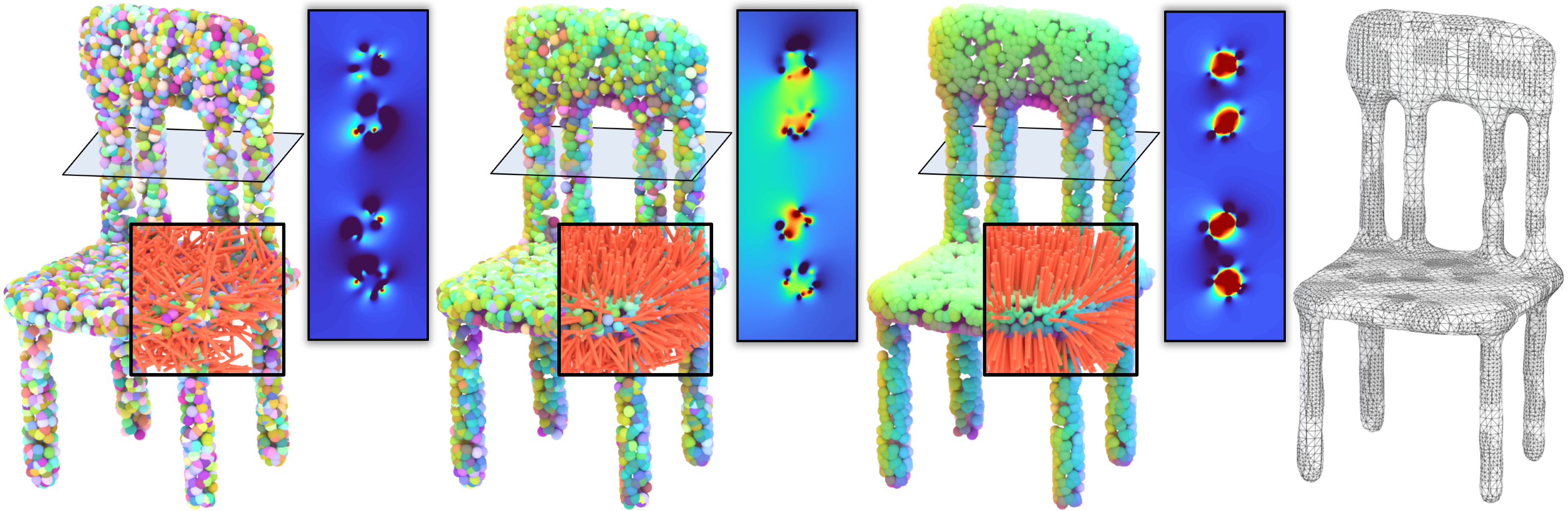
(a) Initial normal vectors                   (b) 20 iterations                        (c) 40 iterations                    (d) Reconstruction

Figure 1. For a closed and orientable surface, the winding number is 0 on the exterior and 1 on the interior. Inspired by this fact, in this paper we consider a reverse problem: given an un-oriented point cloud, is it possible to find the globally consistent normal orientations by regularizing the winding-number distribution? We propose a smooth objective function to characterize the requirements of an acceptable winding-number field. Starting from a set of completely random normals (a), we repeatedly optimize their directions (b,c) until the objective function cannot be reduced. With the computed normals, one can simply call the screened Poisson reconstruction (SPR) solver to produce the final surface (d). Note that we use RGB mapping to visualize the normals and provide a sectional view to visualize the change of the winding-number field, where “blue” and “red” indicate 0 and 1, respectively.

1. Introduction

An unoriented point cloud becomes more informative if it is equipped with a set of normals with globally consistent orientations. Predicting reliable normals serves as a crucial step for many downstream tasks, e.g., surface reconstruction (Kazhdan, 2005; Kazhdan et al., 2006; Kazhdan and Hoppe, 2013; Xu et al., 2022; Wang et al., 2021), shape registration (Pomerleau et al., 2015), determining inside/outside information (Jacobson et al., 2013; Barill et al., 2018), shape analysis (Grilli et al., 2017; Dou et al., 2022; Zapata-Impata et al., 2019). Despite significant progress (Hoppe et al., 1992; Dey and Goswami, 2004; Dey et al., 2005; Alliez et al., 2007; König and Gumhold, 2009; Mérigot et al., 2010; Boltcheva and Lévy, 2017; Guerrero et al., 2018; Li et al., 2022; Hou et al., 2022; Metzer et al., 2021) being made on this problem, it is still a stumbling task of discovering the globally consistent normals for an unoriented point cloud while allowing for various imperfections.

Most of the existing research works (Hoppe et al., 1992; Pauly et al., 2003; Cazals and Pouget, 2005; Alliez et al., 2007; Levin, 1998) first compute a normal tensor for each point, regardless of orientation, followed by spreading the orientation flags through propagation (Metzer et al., 2021). They are not able to deal with various imperfections such as noise, thin structures, nearby surfaces, and sharp features since the normals do not rigorously satisfy the property of spatial coherence. In contrast, the recently proposed iPSR (Hou et al., 2022) and Parametric Gauss Reconstruction (PGR) (Lin et al., 2022) focus more on the global consistency of normal orientations, and achieve better results. However, they still suffer from data sparsity coupled with nearby gaps, thin-walled structures, or highly complex geometry/topology. Fig. 2 demonstrates the results of various approaches, where the red points indicate a false orientation.

\begin{overpic}[width=429.28616pt]{figures/lampall.png} \put(11.0,25.5){{K\"{o}nig} \cite[citeyearpar]{(\@@bibref{Year}{konig2009consistent}{}{})}} \put(43.0,25.5){{PCPNet} \cite[citeyearpar]{(\@@bibref{Year}{guerrero2018pcpnet}{}{})}} \put(77.0,25.5){{Dipole} \cite[citeyearpar]{(\@@bibref{Year}{dipole_propagation}{}{})}} \put(12.0,-3.0){{iPSR} \cite[citeyearpar]{(\@@bibref{Year}{hou2022iterative}{}{})}} \put(45.0,-3.0){{PGR} \cite[citeyearpar]{(\@@bibref{Year}{PGR2022Siyou}{}{})}} \put(83.0,-3.0){{Ours}} \end{overpic}

Figure 2. Existing normal orientation approaches are not able to deal with various imperfections such as noise, thin structures, nearby surfaces and sharp features. Note that the red points indicate a false orientation, i.e., the angle between the ground-truth normal and the predicted normal is larger than $90$ degrees.

In recent years, the winding number, as a powerful tool for inside-outside tests, has gained increasing attention in digital geometry processing, ranging from meshing (Hu et al., 2018) to reconstruction (Barill et al., 2018; Wang et al., 2022b). Despite the ability to distinguish the interior part (the winding number is close to 1) from the exterior part (the winding number is close to 0), it heavily depends on the support of reliable normals. Our hypothesis is that only when the normals are oriented with global consistency, the winding-number field could be approximately binary-valued with $1$ and $0$. This inspires us to optimize the normals such that the winding-number field becomes fully regularized. Based on this hypothesis, we propose an all-in-one functionality to characterize the requirements of a winding-number field from three aspects: (a) the winding number should be close to either $1$ or $0$ at any query point, (b) when the query points are scattered in the neighborhood of input samples $\mathbf{p}_{i}$, the occurrences of $1$ and the occurrences of $0$ should be approximately balanced, and (c) the sample $\mathbf{p}_{i}$’s normal vector should align well with the direction towards the outside Voronoi pole (Amenta and Bern, 1998). Note that the first two requirements are used to regularize the distribution of the winding number while the last requirement enforces the computed normals to be as accurate as the Voronoi-based approaches (Alliez et al., 2007). The three terms can be integrated into a smooth objective function with regard to the normals such that the best configuration of normals can be found by solving an unconstrained optimization.

In the implementation, we use L-BFGS to solve the proposed optimization problem. Starting from a completely random normal setting, it generally requires about $30$-$50$ iterations to arrive at the termination. We use the same set of parameters to test our method on various unoriented point clouds, including synthetic data and real scans. Both quantitative statistics and visual comparison show that our method has the advantage of normal accuracy and consistency. It is not only robust to noise and data sparsity (see Fig. 12 and Fig. 14), but also can handle challenging shapes with complex geometry/topology (see Fig. 19). Furthermore, our method can be even applied to incomplete point clouds that encode an open surface (see Fig. 17). In Fig. 3, we provide a gallery of results produced by our approach.

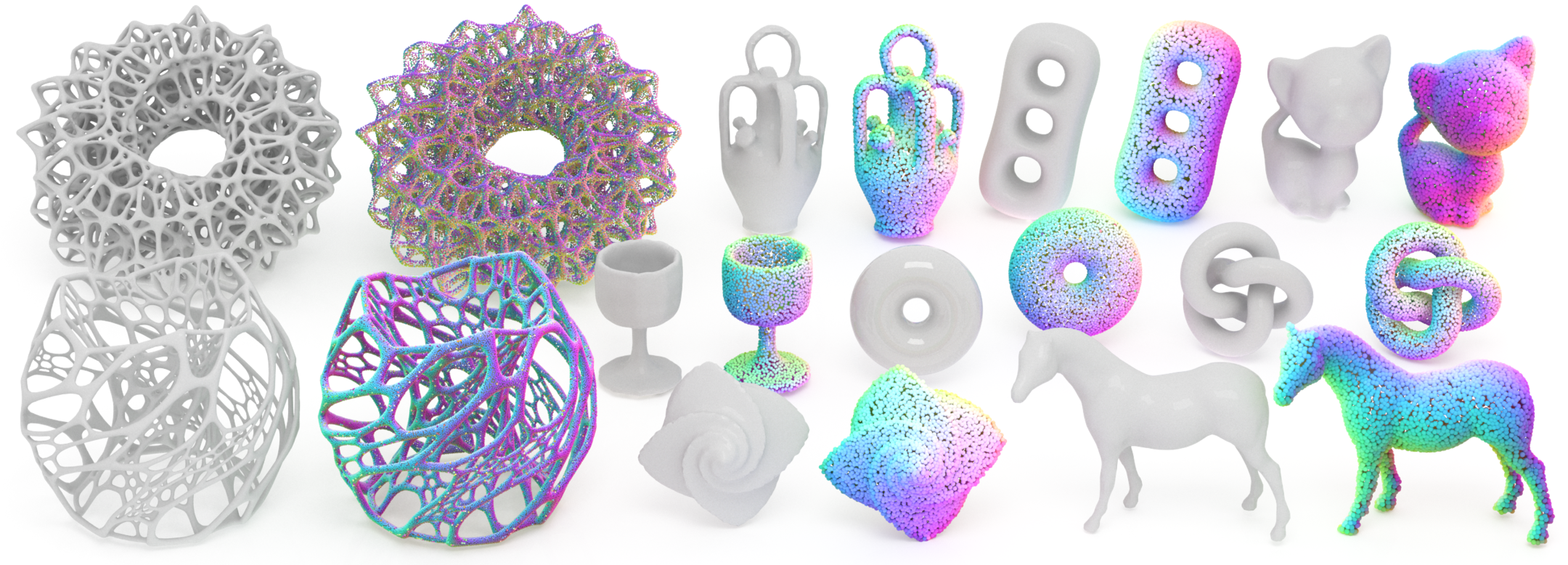
Figure 3. We equip the input unoriented point clouds with our computed normals (rendered with RGB mapping). By feeding the points and the normals together into the screened Poisson reconstruction (SPR) solver, we get high-fidelity reconstruction results (in gray), which exhibit the high quality of the computed normals.

2. Related Work

2.1. Estimating Normal Orientations for Point Clouds

The problem of point cloud orientation has been extensively researched in the past decades. In general, attention must be paid to orientation and accuracy for achieving normal consistency. Existing methods can be divided into two categories: optimization methods and learning techniques. The latter can be further divided into regression-based approaches and surface fitting-based approaches.

Optimization-based Approaches

Hoppe et al. (1992) pioneered on normal orientation. Their approach first uses Principal Component Analysis (PCA) to initialize the normal tensors, and then makes their orientations consistent by a minimum spanning tree (MST) based propagation. Besides the MST-based propagation, more propagation strategies include multi-seed (Xie et al., 2004), Hermite curve (König and Gumhold, 2009), and edge collapse (Jakob et al., 2019). The dipole propagation (Metzer et al., 2021) is also a competing algorithm for propagating the orientation flags. In terms of accuracy improvement, many techniques are proposed, e.g., exponentially decaying function (Levin, 2004), local least square fitting (Mitra and Nguyen, 2003), truncated Taylor expansion (Cazals and Pouget, 2005), moving least squares (Levin, 1998), multi-scale kernel (Aroudj et al., 2017), ensemble framework (Yoon et al., 2007). Wang et al. (2012) proposed to minimize a combination of the Dirichlet energy and the coupled-orthogonality deviation such that the normals are perpendicular to the surface of the underlying shape. In terms of handling sparse data, VIPSS (Huang et al., 2019), as a variational method, reconstructs an implicit surface from an un-oriented point set.

There are also many research works on orienting normal vectors for shapes with corners or geometry edges. For example, L0 norm (Sun et al., 2015) or L1 norm (Sun et al., 2015; Avron et al., 2010) is based on the observation that a general surface is smooth almost everywhere except at some small number of sharp features. As each feature point is allowed to own a range of normal vectors, Zhang et al. (2018) employed the pair consistency voting strategy to compute multiple normals for feature points. Xu et al. (2022) used optimal transport to regularize normal vectors for the points nearby geometry edges. Besides, statistics and subspace segmentation (Li et al., 2010; Zhang et al., 2013; Liu et al., 2015) are used to estimate normals for point clouds with sharp features.

In recent years, much attention has been paid to the global consistency of normal orientations, such as Stochastic Poisson Surface Reconstruction (SPSR) (Sellán and Jacobson, 2022), iterative Poisson Surface Reconstruction (iPSR) (Hou et al., 2022) and Parametric Gauss Reconstruction (PGR) (Lin et al., 2022). For example, iPSR repeatedly refines the surface by feeding the normals computed in the preceding iteration into the Poisson surface reconstruction solver. PGR treats surface normals and surface element areas as unknown parameters, facilitating the Gauss formula to interpret the indicator as a member of some parametric function space. Global methods achieve better results than local methods. However, they still suffer from data sparsity coupled with nearby gaps, thin-walled structures or highly complex geometry/topology. For example, iPSR may disconnect thin structures while PGR may generate bulges for tubular shapes. Furthermore, PGR’s application on large models is constrained by the super-linear growth of GPU memory.

Regression-based Approaches

Regression-based methods model normal estimation as a regression or classification task where the surface normals are directly regressed from the feature extracted from the local patches. Specifically, PCPNet (Guerrero et al., 2018) encodes the multiple-scale features of local patches in a structured manner, which enables one to estimate local shape properties such as normals and curvature. Nesti-Net (Ben-Shabat et al., 2019) estimates the multi-scale property of a point on a local coarse Gaussian grid, which defines a suitable representation for the CNN architecture and enables accurate normal estimation. Zhou et al. (2020) proposed a multi-scale selection strategy to select the most suitable scale for each point through a joint analysis of multiscale features. Hashimoto and Saito (2019) used a point network and a voxel network to estimate normal vectors without sacrificing the inference speed. Although the regression-based methods typically outperform traditional data-independent methods, the regression-based methods rely on a large amount of training data for network training and are limited by the generalization capability because the brute-force training course may cause the network to overfit the normal vectors from the training data.

Surface fitting-based approaches

Different from those regression-based methods, surface fitting-based approaches estimate a fitting surface by taking advantage of its neighboring points. In particular, Lenssen et al. (2020) presented a light-weight graph neural network that parameterizes a local quaternion transformer and a deep kernel function to iteratively re-weight graph edges in a large-scale point neighborhood graph. DeepFit (Ben-Shabat and Gould, 2020) achieves scale-free normal estimation by per-point weight estimation for weighted least squares. Zhu et al. (2021) predicted an additional offset to improve the quality of normal estimation. Recently, the dipole propagation (Metzer et al., 2021) establishes a consistent normal orientation in a local phase and a global phase. However, tests show that dipole cannot deal with the point sparsity or tubular structures.

Although deep learning approaches show great potential in normal estimation, it is still notoriously hard for both point-based regression approaches and surface fitting-based approaches to robustly deal with different noise levels, outliers, thin-plate structures, and varying levels of detail.

2.2. Voronoi-based Normal Orientation

Voronoi diagrams, as a powerful tool to encode spatial proximity, are extensively used to estimate normal vectors (Amenta and Bern, 1998; Dey and Goswami, 2004; Dey et al., 2005; OuYang and Feng, 2005; Alliez et al., 2007; Mérigot et al., 2010; Wang et al., 2012; Boltcheva and Lévy, 2017; Kolluri et al., 2004; Grimm and Smart, 2011). Amenta and Bern (1998) proved that when the point density satisfies the standard of local feature size, one can roughly recover the real normals and even construct a discrete interpolation-type surface that is conformal to the base surface. The central idea is to identify inside poles and outside poles from the Voronoi diagram of the input point cloud, and use the poles to help orient the point cloud and assign their normals. Observing the Voronoi diagram can locally represent the most likely direction of the normal to the surface, Alliez et al. (Alliez et al., 2007) proposed to compute an implicit function by solving a generalized eigenvalue problem. It can be seen from the existing approaches that inside poles and outside poles are robust to noise, which helps find the dominant Delaunay balls in a noise-resistant manner (Dey and Goswami, 2004). Generally speaking, Voronoi diagrams can produce faithful results for dense point clouds but are weak in dealing with thin-plate structures or sharp features. In this paper, we thoroughly investigate the winding number by analyzing all the Voronoi vertices of the input point cloud. Our approach utilizes the winding-number requirements to ensure global normal consistency while relying on the Voronoi diagram to accurately predict the normals.

2.3. Winding Number

The winding number was first introduced by (Meister, 1769). For a smooth manifold surface, it can be computed using a contour integral in complex analysis. As a powerful tool for inside-outside tests, it has been widely used in many higher-level geometry processing operations including tetrahedral meshing (Hu et al., 2020), reconstruction (Barill et al., 2018; Wang et al., 2022b), normal orientation for point clouds (Metzer et al., 2021), shape analysis (Wang et al., 2022a), shape modeling (Sellán et al., 2021), animation (Nuvoli et al., 2022). For example, Jacobson et al. (2013) introduced a winding-number-based function to guide an inside-outside segmentation of a polygonal surface.

Barill et al. (2018) derived a differential form of the winding number function and gave a tree-based fast algorithm to reduce the asymptotic complexity of generalized winding number computation, and also demonstrated a variety of new applications.

It’s known that if the input point cloud is equipped with a meaningful normal setting, the winding number can robustly distinguish the inside from the outside in a global manner and is valued at 1 (inside) and 0 (outside). This observation motivates us to regularize the winding-number field by repeatedly tuning the normals so that they become consistent.

\begin{overpic}[width=429.28616pt]{figures/2_pre/winding2d.png} \put(6.0,-3.5){{(a)~{}Random Normals}} \put(52.0,-3.5){{(b)~{}Ground Truth Normals}} \end{overpic}

Figure 4. (a) If the normals are random, the winding number tends to be $0$ everywhere. (b) If the normals can encode a closed and orientable shape, the winding number is valued at $1$ (interior) and $0$ (exterior).

3. Preliminaries

3.1. Generalized Winding Number

The theory of winding number can be generalized to polygonal meshes (Jacobson et al., 2013), triangle soup and point clouds (Barill et al., 2018). Suppose $\{\mathbf{p}_{i}\}_{i=1}^{N}$ are samples from a continuous surface with normals $\{\mathbf{n}_{i}\}_{i=1}^{N}$. The generalized winding number $w$ at the query point $\mathbf{q}$ can be expressed as an area-weighted sum of the overall contribution of the point set (Barill et al., 2018):

(1) $$w(\mathbf{q})=\sum_{i=1}^{N}a_{i}\frac{(\mathbf{p}_{i}-\mathbf{q})\cdot\mathbf{n}_{i}}{4\pi\left\|(\mathbf{p}_{i}-\mathbf{q})\right\|^{3}},$$

where $a_{i}$ is the dominating area of the point $\mathbf{p}_{i}$. Obviously, the normals are central to the computation of winding numbers. When the normals are random, see Fig. 4 (a), the winding number tends to be $0$ everywhere. If the normals can encode a closed and orientable shape, instead, see Fig. 4 (b), the winding number is about $1$ for the interior points and $0$ for the exterior points.

Remark: How to estimate $a_{i}$ is a problem when the base surface is not available. A commonly used technique (Barill et al., 2018) is to project $\mathbf{p}_{i}$’s $k$-nearest neighbors onto the tangent plane of $\mathbf{p}_{i}$. Thus $a_{i}$ is approximated by the area of the $\mathbf{p}_{i}$’s cell of the 2D Voronoi diagram. However, this strategy depends on the choice of $k$. Since the estimation of $a_{i}$ is essential to the computation of the winding number, we adopt a parameter-free strategy in Sec. 4.4.

3.2. Voronoi Vertices for Examining Winding Number

\begin{overpic}[width=433.62pt]{figures/2_pre/QueryPoints.png} \put(3.0,-3.0){(a)~{}Point cloud} \put(30.0,-3.0){(b)~{}Voronoi vertices} \put(67.0,-3.0){(c)~{}WN distribution} \end{overpic}

Figure 5. Assuming the point cloud is equipped with a ground-truth normal setting, we examine the winding number at the Voronoi vertices of the point cloud. Top row: For a noise-free point cloud, the winding number is close to either $0$ or $1$ for Voronoi vertices. Bottom row: When noises are added to point positions, the histogram of the winding number has a slight change, but still demonstrates two peaks close to 0 and 1. Note that the intersection points between the Voronoi edges and the 1.3x bounding box are also included for the winding number query.

\begin{overpic}[width=433.62pt]{figures/3_method/iter3.png} \vspace{3pt} \put(7.0,0.0){{Random Normals}} \put(33.0,0.0){{4 iterations}} \put(56.0,0.0){{8 iterations}} \put(80.0,0.0){{20 iterations}} \end{overpic}

Figure 6. The optimization progress using our method. The input model is a thin board with randomly initialized normals (in orange) of the point cloud. We cut the board in the middle with a plane to show the sectional view of the winding-number field (visualized in a color-coded style).

The Voronoi diagram (VD) of a set of points $\{\mathbf{p}_{i}\}_{i=1}^{N}$ partitions the entire space into $N$ cells based on spatial proximity. In 3D, it includes Voronoi vertices, Voronoi edges, Voro- noi faces, and Voronoi cells as the atomic elements. Let $\Omega^{vor}_{i}$ be the cell of $\mathbf{p}_{i}$; See the 2D example in the inset figure. The two farthest vertices of $\Omega^{vor}_{i}$, located on both sides of the surface, are defined as poles (Amenta et al., 2001), which are helpful for orienting normals. Note that the inside poles and the outside poles are hard to be distinguished before the normals are determined. Therefore, in this paper, we use all the Voronoi vertices, a superset of the Voronoi poles, for examining the winding number given by a point cloud.

As shown in the top row of Fig. 5(c), the winding number is close to either $0$ or $1$ at the Voronoi vertices for a noise-free point cloud. If we add noises to point positions at a level of 0.5%, the histogram just changes slightly (see the top row of Fig. 5(c)). Note that in Fig. 5 (b), the Voronoi vertices are colored in red (resp. cyan) if the winding number is close to $1$ (resp. $0$). Besides, we use a 1.3x bounding box to enclose the point cloud and add the intersection points between the Voronoi edges and the box as examination points. One may consider a different strategy for generating the examination points, e.g., adding Gaussian noise to the input point cloud. Based on our tests, most of the Voronoi vertices are remote from the surface and noise-insensitive, which accounts for why we take the Voronoi vertices as examination points. We conduct the ablation study in Supplementary Material.

4. Method

The winding number, in its nature, can reflect global inside-outside information, which motivates us to compute the normals by regularizing the winding-number field. In the implementation, we examine the winding number at the Voronoi vertices of the point cloud. We hope that the computed normals can not only lead to a reasonable winding-number field but also accurately align with Voronoi poles. The requirements can be summarized into the following three aspects.

$w(\mathbf{q})$ is valued at 0 or 1.

Although one can construct a surface such that the winding number is valued at any integer, we only consider the common case where the winding number is either $0$ or $1$. We shall include a term $f_{01}(\mathbf{n})$ to characterize the basic requirement of a valid winding-number field.

The winding-number values are balanced for $\mathbf{p}_{i}$’s Voronoi vertices.

Sample $\mathbf{p}_{i}$ dominates a cell in the Voronoi diagram. In general cases, it is unlikely that all the Voronoi vertices of $\mathbf{p}_{i}$’s cell are located inside or outside. Therefore, we hope the number of $1$’s and the number of 0’s are balanced when we consider the winding number of $\mathbf{p}_{i}$’s Voronoi vertices. This observation leads to a balance term $f_{B}(\mathbf{n})$.

Normals align with Voronoi poles.

Like the power crust techniques (Amenta et al., 2001), Voronoi poles are very helpful in predicting the normals. Let $\mathbf{q}_{k}^{i}$ be the $k$-th Voronoi vertex of $\mathbf{p}_{i}$’s Voronoi cell. We hope the vector $\mathbf{q}_{k}^{i}-\mathbf{p}_{i}$ has similar orientation with $\mathbf{n}_{i}$ if $w(\mathbf{q}_{k}^{i})\approx 0$ but reverse orientation with $\mathbf{n}_{i}$ if $w(\mathbf{q}_{k}^{i})\approx 1$. The alignment requirement leads to a term $f_{A}(\mathbf{n})$.

By summarizing them together, we get a functional w.r.t. the normals,

(2) $$f(\mathbf{n})=\frac{f_{01}(\mathbf{n})+\lambda_{B}f_{B}(\mathbf{n})+\lambda_{A}f_{A}(\mathbf{n})}{N},$$

where $\lambda_{B}$ and $\lambda_{A}$ are two parameters to tune the influence of $f_{B}$ and $f_{A}$, respectively. We establish the details of the separate terms in the following subsections, while delaying the ablation study of $\lambda_{B}$ and $\lambda_{A}$ in supplementary material. Fig. 6 gives an example of how the normals change with the decreasing of the value of $f$.

\begin{overpic}[width=433.62pt]{figures/3_method/dw_variance.pdf} \put(5.0,0.0){(a)} \put(59.0,0.0){(b)} \end{overpic}

Figure 7. (a) A standard double well function. (b) A new version with a shear correction for suppressing the randomness of normals.

4.1. The 0-1 Term $f_{01}$

Double well function

In the continuous setting, the winding number is valued at 0 or 1 if the input surface is closed and topologically equivalent to a single-layer orientable surface. Therefore, we need to define an energy function to pull the winding number to the binary states as far as possible. For this purpose, we introduce the double well function inspired by one of the most important functions in the field of quantum mechanics (Jelic and Marsiglio, 2012). A simple form of the double well function can be written as:

(3) $$f_{DW}(x)=4\left(x-0.5\right)^{4}-2\left(x-0.5\right)^{2},$$

with two valleys at $x=0$ and $x=1$, respectively, as Fig. 7(a) shows.

A new double well function with a shear correction

If we equip a point cloud with a set of random normals, the resulting winding number tends to be 0 for an arbitrary query point; See Fig. 4(a). In order to encourage the occurrence of $1$’s for the winding number of examination points, we need to tune the double well function with a shear correction, as Fig. 7(b) shows. In this way, the 0-1 term $f_{01}$ can be defined by the overall contribution of the winding number $w_{j}=w_{j}(\mathbf{n})$ at $\mathbf{q}_{j},j=1,2,\cdots,M.$

(4) $$f_{01}(\mathbf{n})=\sum_{j}^{M}\left(f_{DW}(w_{j})-\frac{w_{j}}{D}\right),$$

where the parameter $D$ is used to tune the degree of shear correction. We make the ablation study about $D$ in the supplementary material and empirically set $D=4$ for all the experiments.

4.2. The Balance Term $f_{B}$

Let $\Omega^{vor}_{i}$ be the Voronoi cell dominated by the point $\mathbf{p}_{i}$ of the point cloud. If the point density meets the local feature size standard (Amenta and Bern, 1998), one half of $\Omega^{vor}_{i}$ is located inside the surface, and the other half is located outside. Therefore, it is reasonable to suppress the occurrence of the situation that all vertices of $\Omega^{vor}_{i}$ are inside the shape or outside the shape. In other words, the winding-number scores at the vertices of $\Omega^{vor}_{i}$ should be balanced, which can be achieved by maximizing the variance of the winding-number scores. Let $\overline{w}^{i}$ be the average score for $\Omega^{vor}_{i}$. The variance can be measured by $\sum_{k}^{M_{i}}(w_{k}^{i}-\overline{w}^{i})^{2}$, where $M_{i}$ is the total number of vertices of $\Omega^{vor}_{i}$, and $w_{k}^{i}=w(\mathbf{q}_{k}^{i})$ is the winding-number score for the $k$-th vertex $\mathbf{q}_{k}^{i}$. The balance term can be defined by the overall winding-number variance.

(5) $$f_{B}(\mathbf{n})=-\sum_{i}^{N}\left(\frac{1}{M_{i}}\sum_{k}^{M_{i}}(w_{k}^{i}-\overline{w}^{i})^{2}\right).$$

4.3. The Alignment Term $f_{A}$

As pointed out in (Amenta and Bern, 1998), Voronoi poles are useful for orienting the normals. Let $\mathbf{p}_{i}$ be a point in the given point cloud, $\mathbf{p}_{i}$’s Voronoi cell $\Omega^{vor}_{i}$ has $M_{i}$ vertices, i.e., $\mathbf{q}_{k}^{i},k=1,2,\cdots,M_{i}$. If $\mathbf{q}_{k}^{i}$ is the inside (resp. outside) pole of $\mathbf{p}_{i}$, $\mathbf{p}_{i}-\mathbf{q}_{k}^{i}$ (resp. $\mathbf{q}_{k}^{i}-\mathbf{p}_{i}$) approximately aligns with the normal vector of $\mathbf{n}_{i}$. In this paper, we turn the observation into an alignment requirement by enforcing the two sequences

$$\mathbf{n}_{i}\cdot(\mathbf{q}_{k}^{i}-\mathbf{p}_{i}),\quad k=1,2,\cdots,M_{i}$$

and

$$w_{k}^{i},\quad k=1,2,\cdots,M_{i}$$

to have exactly the reverse ordering. According to the rearrangement inequality (Hardy et al., 1952), we hope $\sum_{k}^{M_{i}}{w_{k}^{i}}\mathbf{n}_{i}\cdot(\mathbf{q}_{k}^{i}-\mathbf{p}_{i})$ to get minimized. Therefore, we can define the alignment term as follows.

(6) $$f_{A}(\mathbf{n})=\sum_{i}^{N}\left(\frac{1}{M_{i}}\sum_{k}^{M_{i}}{w_{k}^{i}}\mathbf{n}_{i}\cdot(\mathbf{q}_{k}^{i}-\mathbf{p}_{i})\right).$$

\begin{overpic}[width=433.62pt]{figures/3_method/dropline.png} \put(13.0,0.7){$f$} \put(20.0,0.7){$f_{01}$} \put(27.0,0.7){$f_{B}$} \put(35.0,0.7){$f_{A}$} \put(78.0,0.7){$\|g\|$} \end{overpic}

Figure 8. Plot on the decreasing of the functional value and the gradient norm. The experiment is made on the torus model with 4K points.

\begin{overpic}[width=433.62pt]{figures/3_method/distribution.png} \put(21.0,-3.0){(a)~{}Start} \put(72.0,-3.0){(b)~{}End} \end{overpic}

Figure 9. Histograms of winding number distribution for the Voronoi vertices of the torus point clouds, before and after optimization. It can be seen that the distribution of the winding number is regularized by optimization.

Table 1. Statistics on the truth percentages under different sampling conditions and noise levels.

Sampling	White Noise Sampling without noise							White Noise Sampling With 0.25% noise							White Noise Sampling With 0.5% noise
Models	Hoppe	König	PCPNet	Dipole	PGR	iPSR	Ours	Hoppe	König	PCPNet	Dipole	PGR	iPSR	Ours	Hoppe	König	PCPNet	Dipole	PGR	iPSR	Ours
82-block	99.730	99.980	89.300	97.080	99.275	99.175	99.980	84.980	99.900	89.750	98.030	98.800	98.150	99.930	98.950	99.730	89.030	98.230	97.350	98.000	99.880
bunny	99.700	97.080	93.000	94.350	100.000	99.625	99.750	98.550	96.730	92.050	94.930	99.875	99.700	99.980	97.600	96.980	92.630	96.180	99.125	99.375	99.580
chair	69.580	86.730	86.030	80.580	100.000	99.975	100.000	88.030	85.880	86.480	73.550	99.975	100.000	100.000	72.830	65.05	86.430	77.450	99.275	99.400	99.400
cup-22	61.180	60.780	68.450	55.980	99.950	99.400	99.950	93.400	59.380	68.350	56.230	99.925	99.400	99.950	55.930	60.100	67.700	57.900	99.350	98.725	99.850
cup-35	99.800	59.880	83.400	54.400	100.000	100.000	100.000	99.530	60.780	83.00	52.430	99.900	99.950	100.000	99.000	60.830	82.100	53.030	98.725	99.950	100.000
fandisk	98.880	99.850	96.880	86.750	99.725	99.275	100.000	99.480	99.900	96.800	86.700	99.650	99.050	99.950	97.530	99.580	96.850	95.800	98.850	97.325	99.750
holes	100.000	100.000	94.830	90.100	100.000	100.000	100.000	100.000	100.000	94.600	90.900	100.000	100.000	100.000	99.850	100.000	93.750	91.000	99.075	99.975	100.000
horse	95.700	89.700	95.930	90.780	99.425	99.500	99.800	92.680	90.700	95.550	93.080	99.250	99.325	99.750	93.630	89.880	95.530	89.630	96.850	98.425	97.500
kitten	99.680	99.980	94.100	98.230	99.950	99.950	99.980	99.750	100.000	94.050	98.380	99.825	99.950	100.000	99.630	99.980	94.550	97.930	98.150	99.825	99.980
knot	99.850	99.980	80.780	56.230	99.925	100.000	100.000	99.980	99.980	81.380	69.980	98.725	100.000	100.000	99.780	93.730	80.600	70.530	95.300	100.000	99.980
lion	96.380	92.300	94.830	89.980	94.975	97.750	99.700	94.580	93.130	94.880	93.400	93.500	96.325	99.550	88.450	93.330	94.250	88.880	89.325	93.325	94.830
mobius	100.000	55.150	89.800	53.950	100.000	87.250	100.000	68.600	55.130	86.980	54.200	99.175	80.525	99.380	55.980	55.130	82.030	53.650	94.900	68.225	85.780
mug	98.450	66.980	77.350	68.250	99.925	99.875	100.000	98.480	67.480	77.330	67.000	99.925	99.900	100.000	68.230	68.000	76.930	66.150	99.050	99.700	100.000
octa-flower	50.900	88.030	99.280	95.300	98.600	95.350	99.330	53.800	58.180	99.000	95.180	97.725	95.525	98.800	89.330	86.930	98.200	95.500	96.225	93.775	98.550
sheet	51.200	51.130	83.980	52.450	100.000	99.075	100.000	99.480	51.300	83.400	52.700	99.950	98.950	100.000	51.100	51.050	81.130	59.550	99.875	97.225	99.980
torus	100.000	100.000	96.880	99.950	100.000	100.000	100.000	100.000	100.000	96.750	99.980	100.000	100.000	100.000	100.000	100.000	96.780	99.800	99.975	100.000	100.000
trimstar	97.200	100.000	91.050	96.700	98.600	99.650	100.000	99.050	100.000	90.930	94.350	98.150	99.325	100.000	98.880	100.000	91.080	94.830	96.225	98.500	100.000
vase	95.680	90.900	83.330	75.980	99.100	99.825	100.000	94.650	90.130	83.130	82.480	99.000	99.475	100.000	86.430	88.830	82.700	90.700	97.875	98.550	99.650

4.4. Implementation Details

Area weight of $\mathbf{p}_{i}$

Let $\mathbf{p}_{i}$ be a point in the given point cloud. The estimation of the winding number at an arbitrary point has to input the weighting area of $\mathbf{p}_{i}$; See Eq. (1). A typical way for defining the weighting area $a_{i}$ is based on KNN (Barill et al., 2018). However, it has to include a parameter $k$ to resist the irregular distribution of points (typically $k=20$). In this paper, we use a parameter-free strategy for estimating $a_{i}$. As the inset figure shows, $\mathbf{q}_{max}^{i}\in\Omega^{vor}_{i}$ is the farthest Voronoi vertex to $\mathbf{p}_{i}$. We build a plane orthogonal to $\mathbf{q}_{max}^{i}-\mathbf{p}_{i}$ and use it to cut $\Omega^{vor}_{i}$ into two halves, resulting in a convex cut polygon. We use the area of the cut polygon to define $a_{i}$.

Optimization details

The overall objective function takes the normals $\mathbf{n}_{i},i=1,2,\cdots,N,$ as variables. As $\mathbf{n}_{i}$ is required to be a unit vector, we parameterize a normal vector as

(7) $$\mathbf{n}_{i}=\left(\sin(u_{i})\cos(v_{i}),\sin(u_{i})\sin(v_{i}),\cos(u_{i})\right).$$

In this way, we turn the problem of minimizing $f(\mathbf{n})$ into an unconstrained optimization problem.

The function $f=f(\mathbf{n})$ can be viewed as a composite function of

$$f=f(w_{1},w_{2},\cdots,w_{M})$$

and

$$w_{j}=w_{j}(\mathbf{n}_{1},\mathbf{n}_{2},\cdots,\mathbf{n}_{N}).$$

At the same time, $\mathbf{n}_{i}$ is a composite function of $u_{i}$ and $v_{i}$. Therefore, the gradients of the overall function can be quickly computed by the chain rule. We omit the form of the detailed gradients for brevity. Fig. 8 plots how the objective function and the gradient norm are decreased during the optimization. It can be seen from Fig. 9 that the normals become globally consistent upon the regularization of the winding number.

Remark. In order to show that the minimization of $f$ can arrive at the termination, we need to prove the fact that the objective function has a lower bound. Observing that $f_{01}$ is quartic about $w_{j}$ (with a positive leading coefficient) but the other two terms have a lower degree, it is easy to know that $f$ approaches $+\infty$ if one of the winding numbers is sufficiently large, which naturally constrains every $w_{j}$ in a limited range, e.g., $[W_{1},W_{2}]$. Therefore, the boundedness of $f$ follows immediately from the boundedness of $w_{j}$. See more rigorous proof in the supplemental material.

5. Experimental Results

5.1. Experimental Setting

Platform

Our experiments are conducted on a computer with an AMD Ryzen 9 5950X CPU and 32 GB memory. We run the GPU-based approaches (Guerrero et al., 2018; Zhu et al., 2021; Li et al., 2022; Metzer et al., 2021; Lin et al., 2022) on an NVIDIA GeForce RTX 3090 card.

Point clouds and Normalization

We make the tests on a total of 18 models of various shapes (see Table 1). All the point clouds are normalized to a range of $[-0.5,0.5]^{3}$. We use two types of sampling strategies, i.e., white noise sampling and blue noise sampling (Jacobson et al., 2021). Besides the noise-free point clouds, We scale all models to $[-0.5,0.5]^{3}$ so that the longest edge of the bounding box is always 1.0. For noise generation, we use the standard Gaussian distribution with $\mu=0.0$ and $\sigma^{2}=1.0$ to produce noise displacement. Each point is given a random displacement that is added to the original position. The noise level is controlled by a scale factor of $0.25\%$ and $0.5\%$, respectively.

Parameters

In all the experiments, we adopt the same parameter setting: $\lambda_{A}=10.0$, $\lambda_{B}=50.0$, and $D=4.0$. We use the L-BFGS algorithm implemented in C++ for solving the optimization. The termination condition is set by requiring the difference between the objective function values at two consecutive steps not to exceed a threshold of $1.0$.

Approaches

We include five state-of-the-art (SOTA) methods (Hoppe et al., 1992; König and Gumhold, 2009; Metzer et al., 2021; Lin et al., 2022; Guerrero et al., 2018) for comparison. PGR (Lin et al., 2022) receives an un-oriented point cloud as the input and outputs a polygonal surface, but we focus more on the quality of its computed normals. Note that (Hoppe et al., 1992) and (König and Gumhold, 2009) need to pre-compute a Riemannian graph to encode the proximity between points. In our experiments, we take two closely spaced points as neighbors if the distance between them is less than 0.05. Besides, PCPNet (Guerrero et al., 2018) has multiple pre-trained models, we use multi_scale_oriented_normal in all experiments. For PGR (Lin et al., 2022) and Dipole (Metzer et al., 2021), we follow the default setting.

\begin{overpic}[width=429.28616pt]{figures/4_result/normal_comp/normal_comp_ws.png} \put(6.0,-1.5){{Hoppe}} \put(23.0,-1.5){{K{\"{o}}nig}} \put(39.0,-1.5){{PCPNet}} \put(57.0,-1.5){{Dipole}} \put(74.0,-1.5){{PGR}} \put(90.0,-1.5){{Ours}} \end{overpic}

Figure 10. Comparison on the ratio of true normals between our approach and the existing five methods: Hoppe (Hoppe et al., 1992), König (König and Gumhold, 2009), PCPNet (Guerrero et al., 2018), Dipole (Metzer et al., 2021) and PGR (Lin et al., 2022). The true predictions and false predictions are colored in blue and red, respectively. Note that the level of Gaussian noise is $0.5\%$.

\begin{overpic}[width=429.28616pt]{figures/4_result/recon_comp/recon_comp_huapen.png} \put(7.0,-1.0){{Hoppe}} \put(24.0,-1.0){{K{\"{o}}nig}} \put(40.0,-1.0){{PCPNet}} \put(58.0,-1.0){{Dipole}} \put(76.0,-1.0){{PGR}} \put(92.0,-1.0){{Ours}} \put(-1.0,43.0){\rotatebox{90.0}{{BS}}} \put(-1.0,30.0){\rotatebox{90.0}{{WS}}} \put(-1.0,15.0){\rotatebox{90.0}{{WS\_0.25}}} \put(-1.0,3.0){\rotatebox{90.0}{{WS\_0.5}}} \end{overpic}

Figure 11. Visual comparison of the reconstructed surfaces at different sampling conditions and different levels of noise. We show results of four different sampling conditions: BS (blue noise sampling), WS (white noise sampling), WS_0.25 (white noise sampling with 0.25% noise) and WS_0.5 (white noise sampling with 0.5% noise).

5.2. Comparisons

Indicators

We evaluate the performance from two aspects. On the one hand, we keep track of the percentage of correctly oriented normals. For an input point $\mathbf{p}_{i}$, the predicted orientation is true if the angle between the computed normal and the ground-truth normal is less than $90$ degrees. On the other hand, we make statistics about the reconstruction quality by feeding the point clouds and the normals together into the SPR solver (Kazhdan et al., 2006). Specially, we use the Chamfer Distance (CD) to measure the error between the ground-truth surface and the reconstructed surface (with the support of predicted normals).

Quality of predicted normals

In Table 1, we show the statistics of the truth percentages of normals over the $18$ models, under different sampling conditions and noise levels. The statistics show that our approach has a higher truth percentage than the SOTA methods. For example, for the blue noise sampling point clouds, our approach can achieve a percentage of $100\%$ for $88.9\%$ of the tested models, much higher than the SOTA methods. Furthermore, we give a visual comparison in Fig. 10 where the points are colored differently depending on whether the normal orientation is correctly predicted. It can be clearly seen that our approach has an advantage in predicting the normals for points in the tubular regions and thin regions with sharp features and corners; See the highlighted regions.

Besides, we also make statistics about the Root Mean Square Error (RMSE) of angles between the estimated normal and the ground-truth normal, which also shows that our algorithm has advantage in prediction accuracy. The detailed statistics are included in the supplementary material.

Table 2. Reconstruction quality comparison using Poisson surface reconstruction solver (Kazhdan et al., 2006) with predicted normals. The Chamfer Distance between the reconstructed surface and the ground-truth surface is presented scaled by a factor of $100$ for a better presentation.

Sampling	White Noise Sampling without noise							White Noise Sampling With 0.25% noise							White Noise Sampling With 0.5% noise
Models	Hoppe	König	PCPNet	Dipole	PGR	iPSR	Ours	Hoppe	König	PCPNet	Dipole	PGR	iPSR	Ours	Hoppe	König	PCPNet	Dipole	PGR	iPSR	Ours
82-block	0.149	0.149	0.489	0.195	0.158	0.165	0.130	0.593	0.155	0.521	0.184	0.202	0.195	0.134	0.175	0.172	0.578	0.203	0.462	0.244	0.184
bunny	0.143	0.230	0.326	0.358	0.092	0.103	0.112	0.130	0.285	0.355	0.354	0.173	0.156	0.126	0.198	0.285	0.379	0.280	0.322	0.203	0.157
chair	1.758	0.739	0.425	0.583	0.118	0.074	0.076	0.599	0.761	0.461	0.912	0.166	0.116	0.080	1.545	2.311	0.516	0.795	0.397	0.165	0.172
cup-22	1.673	1.631	1.523	1.787	0.121	0.131	0.112	0.338	1.680	1.539	1.778	0.203	0.191	0.139	1.898	1.715	1.568	1.764	0.347	0.267	0.193
cup-35	0.133	1.221	0.903	1.613	0.095	0.115	0.098	0.119	1.215	0.884	1.771	0.171	0.170	0.094	0.147	1.278	0.979	1.721	0.297	0.214	0.134
fandisk	0.128	0.123	0.195	0.637	0.081	0.090	0.073	0.127	0.126	0.211	0.643	0.149	0.120	0.103	0.191	0.171	0.254	0.219	0.307	0.181	0.169
holes	0.036	0.036	0.252	0.286	0.072	0.075	0.073	0.039	0.039	0.267	0.200	0.191	0.144	0.070	0.051	0.051	0.328	0.254	0.576	0.193	0.149
horse	0.291	0.482	0.165	0.307	0.085	0.082	0.075	0.281	0.465	0.192	0.224	0.167	0.088	0.090	0.305	0.522	0.238	0.358	0.454	0.244	0.178
kitten	0.064	0.061	0.268	0.076	0.061	0.099	0.088	0.066	0.065	0.265	0.079	0.177	0.109	0.084	0.073	0.072	0.299	0.092	0.319	0.161	0.144
knot	0.040	0.040	0.817	1.634	0.166	0.105	0.064	0.045	0.046	0.822	0.998	0.338	0.140	0.068	0.063	0.311	0.875	0.931	0.652	0.191	0.123
lion	0.229	0.351	0.211	0.397	0.112	0.117	0.087	0.268	0.349	0.224	0.248	0.268	0.198	0.112	0.388	0.383	0.274	0.365	0.619	0.251	0.228
mobius	0.117	1.551	0.563	1.507	0.126	0.156	0.237	2.161	1.549	0.649	1.529	0.238	0.287	0.417	2.819	1.743	0.755	1.607	0.410	0.435	0.634
mug	0.135	1.228	1.208	1.506	0.135	0.906	0.125	0.146	1.238	1.214	1.514	0.214	0.929	0.118	1.276	1.244	1.253	1.624	0.322	1.240	0.146
octa-flower	2.424	0.601	0.130	0.245	0.093	0.139	0.164	2.445	1.505	0.146	0.232	0.193	0.165	0.177	0.521	0.703	0.181	0.238	0.372	0.293	0.247
sheet	1.607	1.613	3.327	1.563	0.098	0.650	0.091	0.123	1.607	2.909	1.511	0.167	0.717	0.116	1.630	1.635	3.046	1.545	0.380	0.881	0.219
torus	0.019	0.019	0.215	0.019	0.054	0.163	0.043	0.026	0.026	0.232	0.021	0.135	0.190	0.064	0.044	0.044	0.250	0.033	0.264	0.240	0.125
trimstar	0.214	0.137	0.417	0.175	0.158	0.147	0.112	0.154	0.142	0.422	0.208	0.340	0.153	0.110	0.158	0.153	0.454	0.238	0.670	0.225	0.170
vase	0.217	0.440	0.613	0.950	0.094	0.119	0.092	0.243	0.446	0.654	0.611	0.198	0.149	0.107	0.588	0.581	0.727	0.326	0.503	0.194	0.189

\begin{overpic}[width=429.28616pt]{figures/4_result/recon_comp/recon_comp_chair_cup22_lion_vertical.pdf} \put(4.0,-1.0){{Input}} \put(16.0,-1.0){{Hoppe}} \put(28.0,-1.0){{K{\"{o}}nig}} \put(40.0,-1.0){{PCPNet}} \put(53.0,-1.0){{Dipole}} \put(68.0,-1.0){{PGR}} \put(80.0,-1.0){{Ours}} \put(92.0,-1.0){{GT}} \end{overpic}

Figure 12. Comparing the reconstruction quality on point clouds with $0.5\%$ Gaussian noise.

\begin{overpic}[width=424.94574pt]{figures/4_result/varying.png} \put(3.0,-3.0){{(a)~{}Input points}} \put(37.0,-3.0){{(b)~{}Our result}} \put(68.0,-3.0){{(c)~{}Reconstruction}} \end{overpic}

Figure 13. We construct a point cloud of the genus-3 torus with varying point densities (colored in varying darkness). Both the predicted normals and the reconstructed surface show that our approach is robust to the point density.

Quality of reconstructed surfaces

We further take the SPR solver as a blackbox to observe the reconstruction quality. For a fair comparison, we capture the normals of PGR (Lin et al., 2022) and feed the oriented point set into the SPR solver. In fact, the original reconstruction strategy of PGR uses iso-surfacing to extract reconstructed surfaces and tends to produce over-smooth results. By comparison, SPR is better than iso-surfacing in preserving geometric details for normals of the same quality. A basic fact is that better normals lead to better-reconstructed surfaces. We record the statistics about the reconstruction quality in Table 2. Note that the Chamfer Distance between the reconstructed surface and the ground-truth surface is scaled by $100$ times for a better presentation. The statistics show that for most of the 18 models, our predicted normals produce the best reconstruction quality. For example, when the point sets are added by $0.5\%$ Gaussian noise, our method has the best scores on $55\%$ of the models. Based on the scores, the three top-ranked approaches are ours, König (König and Gumhold, 2009) and Hoppe (Hoppe et al., 1992), respectively.

Furthermore, we use Fig. 11 to visually compare reconstruction results on the Vase model at various sampling conditions and noise levels. It can be seen that from the reconstructed surfaces our approach can infer the normals, with the highest fidelity. Especially, even if the noise level amounts to 0.5%, our method can still produce a faithful result; See the handles of the Vase model.

\begin{overpic}[width=429.28616pt]{figures/4_result/lowsampling.png} \put(3.0,-1.0){{Input}} \put(15.0,-1.0){{Hoppe}} \put(29.0,-1.0){{K{\"{o}}nig}} \put(42.0,-1.0){{PCPNet}} \put(56.0,-1.0){{Dipole}} \put(69.0,-1.0){{PGR}} \put(81.0,-1.0){{Ours}} \put(94.0,-1.0){{GT}} \put(-1.5,22.0){\rotatebox{90.0}{{500 points}}} \put(-1.5,12.0){\rotatebox{90.0}{{750 points}}} \put(-1.5,1.5){\rotatebox{90.0}{{1K points}}} \end{overpic}

Figure 14. Tests are made on sparse point clouds: $500$ points, $750$ points and $1$K points. Our results are close to the ground truth for each of the three inputs. The comparison shows that our algorithm has a big advantage on sparse raw data. We also mark clearly the Chamfer Distance (CD) scores between the reconstructed surface and the ground-truth surface for a quantitative comparison. Note each CD score is scaled by a factor of 100.

\begin{overpic}[width=429.28616pt]{figures/4_result/normal_comp/normal_comp.png} \put(5.0,-1.5){{Hoppe}} \put(22.0,-1.5){{K{\"{o}}nig}} \put(39.0,-1.5){{PCPNet}} \put(55.0,-1.5){{Dipole}} \put(72.0,-1.5){{PGR}} \put(89.0,-1.5){{Ours}} \put(-1.5,39.0){\rotatebox{90.0}{{BS}}} \put(-1.5,28.0){\rotatebox{90.0}{{WS}}} \put(-1.5,14.0){\rotatebox{90.0}{{WS\_0.25}}} \put(-1.5,3.0){\rotatebox{90.0}{{WS\_0.5}}} \end{overpic}

Figure 15. The Chair model contains thin-walled tubes and plates, as well as nearby gaps (see the highlighted region). Our approach can yield the highest truth percentage among the five approaches. Note that the false predictions are colored in red.

5.3. Noise, Varying Point Density and Data Sparsity

Noise

In Fig. 12, we add $0.5\%$ Gaussian noise to the point clouds of the Cup model, the Chair model, and the Lion model, to test the noise-resistant ability. It can be clearly seen from the visual comparison that our algorithm has a better noise-resistant ability. Specially, our algorithm can provide faithful normals on the back and the legs of the Chair model, even in presence of serious noise. Two reasons account for the noise-resistant property. First, we examine the winding number at the Voronoi vertices whose positions are robust to small variations of the original point cloud, especially for those Voronoi vertices distant to the surface. Second, the whole optimization framework is built on the regularization of the winding number, and thus can capture the normal consistency from a global perspective.

Varying point density

In Fig. 13, we construct a point cloud with varying point density (colored in varying darkness). We intend to use this example to test if our algorithm can deal with irregular point distributions. Recall that Eq. (1) includes an area weight $a_{i}$, which has a serious influence on the estimation accuracy of the winding number. We give an intuitive technique for estimating $a_{i}$ based on the Voronoi diagram; See Section 4.4. The technique is parameter-free and computationally efficient. It can be seen from Fig. 13 that both the predicted normals and the reconstructed surface have a high quality, which shows that the estimation of $a_{i}$ is independent of the point density.

Data sparsity

In Fig. 14, we have three sparse point clouds, and the numbers of points are respectively 500, 750, and 1K. We intend to use this example to test the performance on sparse inputs , since when there are nearby gaps and thin-walled tubes/plates, data sparsity will inevitably double the difficulty of predicting normals. It can be clearly seen from the visual comparison that our results are close to the ground-truth for each of the three inputs.

5.4. Nearby Gaps, Thin Plates/Tubes, and Sharp Angles

Nearby gaps and thin plates/tubes

For our approach, the strength in dealing with thin tubes has been validated on the Vase model shown in Fig. 11. In Fig. 15, we give four versions of the Chair point cloud to evaluate how well it handles nearby gaps and thin plates/tubes. As can be observed, our approach noticeably outperforms the SOTA methods in addressing these flaws (see the highlighted region), which is due to the global property inherited from the winding number.

\begin{overpic}[width=429.28616pt]{figures/4_result/sharpangles.png} \put(6.0,23.0){{(a)~{}30 degrees}} \put(39.0,23.0){{(b)~{}20 degrees}} \put(73.0,23.0){{(c)~{}15 degrees}} \put(1.0,-3.0){{(d)~{}Random normals}} \put(40.0,-3.0){{(e)~{}Our result}} \put(68.0,-3.0){{(f)~{}Reconstruction}} \end{overpic}

Figure 16. (a-c) Our approach can estimate normals accurately even if the angles are as small as 15 degrees. (d-f) For the Airplane model with sharp angles, we show the initial normals, the optimized normals, and the faithfully reconstructed result.

Sharp angles

The existence of sharp angles is one of the challenges for orienting a raw point cloud. In the top row of Fig. 16, we show three toy models with different dihedral angles. It can be seen that our approach can estimate normals accurately even if the angles are as small as 15 degrees. We also use the Airplane model to test the ability to deal with sharp angles. Both the optimized normals and the faithfully reconstructed result show that our algorithm can produce a desirable result for point clouds with sharp angles. The contrast in the bottom row of Fig. 14 also validates the effectiveness of our approach in coping with sharp angles. It’s worth pointing out that the propagation-based methods (Metzer et al., 2021) rely on the assumption of spatial coherence, which does not hold when sharp angles exist, and thus fail to fully capture the global context of the shape in presence of sharp angles.

\begin{overpic}[width=433.62pt]{figures/4_result/open.png} \put(13.0,-3.0){{(a)~{}PGR}} \put(45.0,-3.0){{(b)~{}iPSR}} \put(78.0,-3.0){{(c)~{}Ours}} \end{overpic}

Figure 17. Comparing PGR, iPSR, and ours on estimating normals for an open-surface point cloud. iPSR does not support open surfaces. PGR fails to report reliable normals for the boundary points. However, our estimated normals comply with the real shape at both the interior points and the boundary points.

\begin{overpic}[width=429.28616pt]{figures/4_result/linetype.png} \put(-2.0,88.0){\rotatebox{90.0}{{Input}}} \put(-2.0,63.0){\rotatebox{90.0}{{PGR Normal}}} \put(-2.0,41.0){\rotatebox{90.0}{{Our Normal}}} \put(-2.0,22.0){\rotatebox{90.0}{{PGR Recon}}} \put(-2.0,3.0){\rotatebox{90.0}{{Our Recon}}} \end{overpic}

Figure 18. Normal estimation for wireframe-type point clouds. All the models are from VIPSS (Huang et al., 2019). PGR may produce bulges around thin tubular structures.

\begin{overpic}[width=429.28616pt]{figures/4_result/diffcultmodels.png} \put(5.0,0.0){{Input}} \put(17.0,0.0){{Hoppe}} \put(30.0,0.0){{K{\"{o}}nig}} \put(42.0,0.0){{PCPNet}} \put(57.0,0.0){{Dipole}} \put(71.0,0.0){{iPSR}} \put(92.0,0.0){{Ours}} \end{overpic}

Figure 19. Tests on point clouds with highly complex topology/geometry. The model in the top row has 80K points while the model in the bottom row has 100K points. Note that PGR runs out of GPU memory on an NVIDIA GeForce RTX 3090 graphics card. Chamfer Distance (CD) between the reconstructed surface and the ground-truth surface is marked for a quantitative comparison. Note each CD value is scaled by a factor of 100.

\begin{overpic}[width=390.25534pt]{figures/4_result/real_scan.png} \put(10.0,-4.0){{Input}} \put(33.0,-4.0){{Normal Encoding}} \put(67.0,-4.0){{Reconstruction}} \end{overpic}

Figure 20. The three raw point clouds are real scans downloaded from (Huang et al., 2022) dataset. Each of them is downsampled to 10K points. From the color-coded visualization of normals, as well as the reconstructed surfaces, we can see that our method can deal with real scans.

5.5. Open Surfaces, Wireframes, Complex Topology and Real Scans

Open-surface Point Cloud

In Fig. 17, we sample a point set from an open surface. We compare PGR, iPSR, and ours on estimating normals on the open-surface point cloud. iPSR does not support open surfaces. PGR fails to report reliable normals for the boundary points since it assumes the closed surface. In contrast, our estimated normals comply with the real shape at both the interior points and the boundary points.

On one hand, the winding number is still indicative for open surfaces (Jacobson et al., 2013; Chi and Song, 2021). On the other hand, the three terms in our objective function do not assume the closedness of the surface. Recall that we include the intersections between the 1.3x bounding box and the Voronoi diagram as examination points. If the input point set encodes a closed surface, it is proper to deem the intersections as outside points and enforce the winding number at the intersections to be 0. But for open surfaces, the constraint cannot be specified. Therefore, in our implementation, we do not specify the requirements in all our experiments.

Wireframes

Wireframes serve as a kind of compact skeletal representation of a real-world object. Due to the extreme data sparsity, the SOTA methods fail to correctly predict the normals. Unlike patch-based normal fitting (Metzer et al., 2021), our approach aims at evaluating the global normal consistency by computing the overall contribution of each point. The experimental results in Fig. 18 show that both our method and PGR are capable of handling the wireframe-type inputs, but PGR may produce bulges around thin tubular structures (see the highlighted window).

Highly complex structures

Fig. 19 shows two nest-like models with complex topology/geometry. The point cloud in the top row has 80K points while the point cloud in the bottom row has 100K points. It can be seen that all five SOTA methods fail on the two highly complex models. iPSR (Hou et al., 2022) depends on the initialization of normals. For a shape with complicated topology/geometry, iPSR cannot reverse the false normals to the correct configuration, and thus easily cause disconnection or adhesion, especially around thin structures. PGR is not GPU-memory friendly (superlinear growth w.r.t. the number of points) and runs out of memory when the input point cloud reaches 80K points (note that we test PGR on an NVIDIA GeForce RTX 3090 graphics card with 24GB of GPU memory). In contrast, our method can deal with complicated geometry/topology and faithfully recover the normal vectors.

Real scans

Fig. 20 shows three raw point clouds, each of which is down-sampled to 10K points. From the color-coded visualization of normals, as well as the reconstructed surfaces, it can be seen that our method can effectively orient the normals for real-life objects, which validates the usefulness of our algorithm in practical scenarios.

\begin{overpic}[width=433.62pt]{figures/4_result/psr.png} \put(8.0,-4.0){{Input}} \put(33.0,-4.0){{PGR\_1}} \put(58.0,-4.0){{PGR\_2}} \put(84.0,-4.0){{Ours}} \end{overpic}

Figure 21. Two parameter settings of PGR (Lin et al., 2022). PGR_1: wmin=0.04, alpha=2.0. PGR_2: wmin=0.0015, alpha=1.05.

5.6. Discussion on Global Methods

In the following, we make a discussion on the global methods including iPSR (Hou et al., 2022), PGR (Lin et al., 2022) and ours.

Ours v.s. iPSR

iPSR, as a global method, is excellent in estimating oriented normals. Benefiting from Poisson surface reconstruction, it has many nice features. In its nature, iPSR gets more and more prior during the iterations of the reconstruction surface. If the given raw data does not have serious imperfections or challenging structures, iPSR can produce desirable normals, as well as a high-quality reconstruction surface. On the flip side, iPSR inherits some disadvantages of Poisson surface reconstruction. For example, iPSR cannot deal with the point clouds of an open surface, as shown in Fig. 17. Additionally, when the point clouds are as complex as Fig. 19, iPSR cannot reverse the false normals to the correct configuration and easily cause disconnection or adhesion, especially around thin structures. To summarize, the biggest weakness of iPSR lies in that if the initial surface is much different from the target surface, the structural/topological issues are hard to be fixed.

Ours v.s. PGR

First, in the original paper of PGR, the authors recommend several groups of parameters, depending on the number of points in the raw data. In contrast, our parameters remain the same for all the experiments, independent of the size of the raw data. Second, the statistics (available in the supplementary material) show that our method has better accuracy in predicting normals due to the alignment term that enforces the normals to point toward outside Voronoi poles, whereas, the inaccurate normals produced by PGR weaken the ability of fidelity preserving. Fig. 21 shows that the inaccurate normals of PGR cause a failure in recovering the center hole of the star shape, and any recommended parameters. Finally, PGR incurs a quadratic complexity of computational time and memory footprint, which limits its practical usage , especially on large models. For example, PGR fails to deal with the complex shapes shown in Fig. 19.

5.7. Run-time Performance

We provide the run-time performance statistics in Table 3. The tests are made on the torus model with different resolutions ranging from $0.5K$ points to $10K$ points. The total running time mainly consists of the construction of the Voronoi diagram and the optimization. It can be seen that optimization is the most time-consuming stage due to (1) the number of variables is twice as large as the number of the points, and (2) the objective function has to be evaluated by a double loop, i.e., over each $\mathbf{p}_{i}$ and each $\mathbf{q}_{j}$, leading to a non-linear climbing in the computational overhead. But we must point out that even for the Torus model with 10K points, generally, 50 iterations, computed in 10 minutes, suffice to arrive at the termination. The overhead is acceptable for many non-real-time geometry processing tasks.

Table 3. Running time (in seconds) of different methods w.r.t. the number of points #V. We test with the Torus model.

#V	0.5K	1K	3K	5K	7K	10K
Hoppe	0.324	0.477	0.625	0.967	1.112	1.569
König	0.306	0.353	0.625	0.815	1.017	1.185
PCPNet	4.226	5.446	6.388	8.753	11.015	12.581
Dipole	3.277	3.565	5.489	8.411	11.602	14.517
PGR	0.228	0.260	0.489	0.612	0.823	1.020
iPSR	2.801	3.535	4.321	4.543	4.476	5.173
Ours	5.240	15.499	72.434	174.541	282.294	559.854

\begin{overpic}[width=433.62pt]{figures/4_result/recon_comp/Comp_ispr.png} \put(2.0,-3.5){{(a)~{}Input}} \put(43.0,-3.5){{(b)~{}iPSR}} \put(84.0,-3.5){{(c)~{}Ours}} \end{overpic}

Figure 22. We sample 3K points from the Lamp model ShapeNet (Chang et al., 2015). Compared with iPSR (Hou et al., 2022), our method produces better reconstruction quality. However, the highlighted part shows that our predicted normals are not very accurate, leading to a conspicuous artifact in the reconstructed surface.

6. Limitations and Future Work

The first limitation lies in the run-time performance. As we have to repeatedly evaluate the winding number for each data point and each query point, the timing cost spent in a single computation of the objective function amounts to $O(NM)$, where $N$ and $M$ are respectively the number of data points and the number of query points. To alleviate this, one could downsample the input point set. After the normals of the subset are estimated, the un-oriented points can get normals by a simple propagation. Another direction of boosting the run-time performance is to develop a GPU version to further improve the parallelism.

The second limitation is that there is room for further improvement in the accuracy of predicted normals. In Fig. 22, we sample 3K points on the Lamp model from ShapeNet (Chang et al., 2015). Our predicted normals are much different from the ground-truth normals, in spite of being better than iPSR (Hou et al., 2022). The inaccurate normals lead to a conspicuous artifact in the reconstructed surface. In the future, we shall further improve the prediction accuracy based on prior knowledge about the geometry/topology.

Finally, our method may fail when there are many points scattered inside the volume, or a high-density point cloud is coupled with high-level noise. Both situations may violate the $0-1$ balance requirement, potentially resulting in a failure case. To address these challenges, it is necessary to develop some pre-processing techniques to filter out those points that do not contribute to the underlying surface at all.

7. Conclusion

This paper presents a globally consistent normal orientation method by regularizing the winding-number field. We formulate the normal orientation problem into an optimization-driven framework that considers three requirements in the objective function, two of which specify requirements on the winding-number field and the other term constraining the alignment with Voronoi poles. We conduct extensive experiments on point clouds with various imperfections and challenges, such as noise, data sparsity, nearby gaps, thin-walled plates, and highly complex geometry/topology. Experimental results exhibit the advantage of the proposed approach.

Appendix

Appendix A $f$ Has a Lower Bound

In order to show that the minimization of $f(\mathbf{n})$ (see Eq. (2) in the paper) can arrive at the termination, we need to prove why the objective function has a lower bound.

Recall that $f(\mathbf{n})$ has three terms $f_{01}$, $f_{A}$ and $f_{B}$. By assuming that the maximum of $\|\mathbf{q}_{k}^{i}-\mathbf{p}_{i}\|$ is $L$, the diagonal length of the enclosing box, we have

(8) $$\begin{split}|f_{A}(\mathbf{n})|&\leq\sum_{i}^{N}\left|\frac{1}{M_{i}}\sum_{k}^{M_{i}}{w_{k}^{i}}\mathbf{n}_{i}\cdot(\mathbf{q}_{k}^{i}-\mathbf{p}_{i})\right|\\ &\leq\sum_{i}^{N}\left(\frac{L}{M_{i}}\sum_{k}^{M_{i}}{|w_{k}^{i}|}\right).\end{split}$$

Therefore, it is easy to show that $f_{01}$ is quartic about $w_{j}$ while $f_{A}$ and $f_{B}$ can be bounded by a lower-degree polynomial function about $w_{j}$. Suppose that $w_{j}$ goes to $+\infty$ or $-\infty$. $f_{01}$ must approach $+\infty$ in either case. Considering that $f_{01}$ has a higher rate of change than $f_{A}$ and $f_{B}$, we can conclude that when $w_{j}$ goes to $+\infty$ or $-\infty$, the overall value of $f(\mathbf{n})$ must approach $+\infty$. As our goal is to minimize $f(\mathbf{n})$, $w_{j}$ must be naturally constrained to a limited range of $[W_{1},W_{2}]$. The boundedness of $f(\mathbf{n})$ can be immediately verified based on the fact that $f(\mathbf{n})$ is a continuous function in the closed interval $[W_{1},W_{2}]$.

Appendix B More Comparison

Table 4. Comparison of the angle RMSE with the SOTA methods at different sampling conditions.

Sampling	Blue Noise Sampling						White Noise Sampling						White Noise Sampling With 0.25% noise						White Noise Sampling With 0.5% noise
Models	Hoppe	König	PCPNet	Dipole	PGR	Ours	Hoppe	König	PCPNet	Dipole	PGR	Ours	Hoppe	König	PCPNet	Dipole	PGR	Ours	Hoppe	König	PCPNet	Dipole	PGR	Ours
82-block	117.870	20.191	52.218	24.837	30.611	18.631	22.972	21.895	57.822	36.191	30.903	19.890	67.967	22.214	58.451	32.666	55.719	22.205	27.425	23.005	60.602	32.170	77.330	27.192
bunny	25.051	33.147	45.505	35.795	19.388	23.581	17.652	30.446	48.111	41.014	21.082	18.473	24.560	33.488	49.925	38.942	51.351	17.334	28.607	32.378	50.139	34.774	73.198	24.735
chair	98.024	96.834	60.557	105.177	18.597	9.324	92.216	60.172	62.560	74.170	20.653	12.178	57.527	60.761	62.651	86.063	65.082	16.434	84.449	96.390	63.778	77.731	86.572	32.448
cup-22	18.583	107.427	88.692	109.907	17.573	9.227	103.229	103.407	89.561	107.211	24.954	13.710	44.816	104.835	90.176	106.561	48.635	14.220	109.334	103.585	90.580	104.788	69.075	20.870
cup-35	10.453	89.978	67.295	120.922	19.711	9.610	15.208	108.913	66.949	112.636	21.614	11.080	17.309	107.568	67.185	114.834	49.497	12.680	21.296	106.810	69.896	113.894	71.405	19.041
fandisk	111.246	19.243	32.898	31.515	24.190	15.095	25.464	21.070	37.061	63.276	24.943	18.852	23.148	21.158	37.920	63.270	53.196	20.392	31.770	27.474	40.835	39.086	76.762	22.594
holes	5.428	5.428	39.000	42.304	21.160	20.879	6.225	6.225	42.841	55.063	21.032	9.730	6.667	6.667	44.039	52.910	59.078	12.778	10.283	7.836	47.739	52.236	83.886	24.310
horse	33.319	47.994	31.786	46.661	24.270	23.428	36.567	51.363	37.052	49.740	22.636	17.222	45.777	50.092	39.566	44.637	66.504	21.637	42.982	51.202	41.717	53.306	88.838	39.494
kitten	16.164	9.882	36.495	28.360	18.149	12.834	13.994	11.001	43.810	25.569	19.388	12.335	13.970	11.249	44.775	24.671	59.984	14.473	14.873	11.980	45.921	27.288	80.554	23.598
knot	4.634	6.012	71.819	87.369	31.773	5.291	8.174	6.838	70.257	116.168	29.990	6.121	7.929	7.773	69.993	95.297	57.246	10.086	10.336	44.105	71.110	93.984	77.715	17.086
lion	39.775	48.542	40.831	55.493	47.223	32.986	42.277	52.103	44.106	55.818	44.638	23.621	46.637	49.633	45.442	48.789	75.879	30.074	59.319	50.398	49.112	59.108	91.063	52.139
mobius	26.234	122.025	53.639	120.832	21.448	29.550	27.995	121.133	55.871	118.247	26.797	28.346	102.424	120.963	61.251	117.930	60.265	49.081	119.506	120.518	71.101	117.068	73.098	88.530
mug	12.380	99.870	78.598	94.666	20.618	9.458	22.274	99.145	77.615	92.522	26.271	11.399	22.743	97.616	77.761	93.732	47.326	12.412	95.910	96.303	77.940	95.133	65.508	17.144
octa-flower	115.579	63.804	21.108	31.533	27.405	30.227	115.992	60.782	27.439	41.275	28.288	42.195	112.586	105.038	30.186	41.486	59.050	88.270	56.832	62.286	35.594	40.633	80.510	39.684
sheet	121.675	121.682	69.920	117.485	29.288	26.978	119.934	119.905	68.632	110.042	19.913	16.290	23.038	119.754	69.260	109.920	61.542	20.229	119.582	119.680	73.599	102.809	87.584	32.310
torus	3.239	3.239	30.858	19.187	13.481	12.493	3.723	3.723	35.484	5.376	14.901	7.455	4.167	4.167	36.483	4.775	48.894	11.288	5.510	5.510	38.420	9.096	72.588	19.166
trim-star	24.069	18.808	48.281	43.216	29.519	17.774	34.325	20.377	51.527	35.829	31.829	17.275	25.209	20.848	52.233	43.734	61.031	19.974	26.540	21.339	53.525	42.390	81.154	27.245
vase	39.500	48.036	66.198	59.083	21.234	13.957	38.677	52.584	66.170	80.204	23.450	14.656	41.840	53.557	66.856	69.580	62.990	18.694	61.422	57.240	68.643	52.113	86.423	29.463

Table 5. Comparison of normal orientation with three normal estimation methods.

Sampling	Blue Noise Sampling				White Noise Sampling				0.25% noise White Noise Sampling				0.5% noise White Noise Sampling
Models	PCA	AdaFit	NeAF	Ours	PCA	AdaFit	NeAF	Ours	PCA	AdaFit	NeAF	Ours	PCA	AdaFit	NeAF	Ours
82-block	75.950	50.150	51.800	100.000	75.675	50.675	51.225	99.980	75.625	51.225	52.250	99.930	75.825	52.050	53.650	99.880
bunny	89.750	51.375	50.375	100.000	89.800	51.375	50.125	99.750	89.725	50.475	50.300	99.980	89.775	50.850	50.800	99.580
chair	62.775	53.125	50.625	100.000	64.250	52.750	50.100	100.000	63.575	52.825	54.000	100.000	64.825	52.125	51.050	99.400
cup-22	58.425	52.225	52.000	100.000	58.175	50.075	51.550	99.950	58.550	50.150	51.325	99.950	58.450	50.550	50.175	99.850
cup-35	66.775	50.775	51.550	100.000	67.725	50.525	50.350	100.000	68.025	50.200	52.250	100.000	67.600	51.450	53.650	100.000
fandisk	90.200	54.950	50.700	100.000	90.000	55.075	50.975	100.000	90.050	54.675	50.675	99.950	89.975	54.775	51.650	99.750
holes	79.275	50.575	51.325	100.000	79.350	51.200	51.175	100.000	79.650	51.575	50.675	100.000	79.075	50.900	51.650	100.000
horse	81.875	50.200	50.600	99.500	80.275	51.050	50.500	99.800	80.800	50.350	51.800	99.750	80.625	51.350	51.025	97.500
kitten	90.977	55.011	51.937	100.000	91.075	57.325	51.750	99.980	90.975	57.625	53.875	100.000	90.950	57.100	51.250	99.980
knot	72.975	50.100	51.050	100.000	72.750	50.825	50.250	100.000	72.875	50.925	52.100	100.000	72.275	50.775	51.850	99.980
lion	85.275	53.025	52.125	99.380	84.900	54.575	50.275	99.700	85.200	54.750	52.625	99.550	85.475	55.775	51.850	93.830
mobius	55.225	53.700	53.050	100.000	55.425	54.575	54.625	100.000	55.500	53.800	52.500	97.380	54.875	53.825	52.650	85.780
mug	64.775	50.575	53.525	100.000	67.250	50.650	50.875	100.000	67.225	50.825	52.125	100.000	66.825	51.000	52.950	100.000
octa-flower	98.800	50.275	51.750	100.000	94.750	51.550	53.050	99.330	94.650	51.525	50.900	98.800	94.775	51.700	51.800	98.550
sheet	83.600	54.425	56.400	100.000	71.575	51.925	51.625	100.000	71.750	51.550	51.775	99.950	71.325	51.775	52.000	98.980
torus	89.225	50.125	53.800	100.000	89.950	50.500	52.100	100.000	89.950	50.350	51.000	100.000	90.125	50.225	50.400	100.000
trimstar	80.975	50.300	52.625	100.000	81.150	50.325	53.475	100.000	81.125	51.250	50.750	100.000	81.250	51.375	51.175	100.000
vase	84.575	53.400	50.375	100.000	86.350	51.825	50.250	100.000	86.725	52.050	51.475	100.000	86.275	52.500	50.450	99.650

Angle RMSE

In the main paper, we give the statistics about the ratio of true normals. Here we further give the statistics about the Root Mean Square Error (RMSE) of the angles between the estimated normals and the ground truth normals.

Normal Evaluation Using Angle RMSE

In Sec. 5.4, we give a visual comparison to exhibit the noise-resistant ability of our approach compared with the SOTA methods (Metzer et al., 2021; Hoppe et al., 1992; König and Gumhold, 2009; Guerrero et al., 2018; Lin et al., 2022). We report the angle RMSE statistics under four different sampling conditions in Table 4. It can be clearly seen that our method surpasses the other methods in terms of normal orientations. Even if the noise level amounts to $0.5\%$, our method can still get the best score for $55\%$ of the models, and a competitive score for another $40\%$. For example, the best score ($10.336$) is given by Hoppe on the Knot model, and ours is the second best ($17.086$), which is much better than the remaining scores $44.105$, $71.110$ and $93.984$.

There are some methods such as PCA (Rusu and Cousins, 2011), AdaFit (Zhu et al., 2021) and NeAF (Li et al., 2022) that focus on normal estimation. We also include them for comparison; See the statistics in Table 5. The statistics show that our algorithm has a big advantage of prediction accuracy over the SOTA methods, on all the $18$ models and under all the $4$ noise sampling conditions.

\begin{overpic}[width=429.28616pt]{figures/4_result/abla_voronoi.png} \put(3.0,-3.0){Random $r=0.1$} \put(37.0,-3.0){Random $r=0.2$} \put(70.0,-3.0){Voronoi vertices} \end{overpic}

Figure 23. In order to test different sampling strategies, we generate Gaussian noise near the point cloud (radius $r=0.1$ or $0.2$) to produce examination points. First column: $r=0.1$ (top: examination points; bottom: normals). Second column: $r=0.2$ (top: examination points; bottom: normals). Last column: Voronoi vertices as examination points. It can be seen that Voronoi vertices are more suitable for serving as the examination points. Note that we iterate $200$ steps for $r=0.1,0.2$ and $40$ steps for the situation of Voronoi vertices as examination points.

Appendix C Strategies for Generating Examination Points

We conduct the ablation study about different strategies for generating examination points. Specially, we compare our Voronoi-based sampling strategy with the off-surface random sampling strategy. As shown in Fig. 23, we randomly sample points around the surface of the shape with two sampling radii $r=0.1$ and $r=0.2$. Note that we iterate $200$ steps for $r=0.1,0.2$ and $40$ steps for the situation of Voronoi vertices as examination points. It can be seen that Voronoi vertices are more suitable for serving as the examination points. The superiority of Voronoi-based sampling is due to the fact that the majority of Voronoi vertices are located either deepest inside the surface, or furthest outside the surface (approximating the inner and outer medial axis (Amenta et al., 2001)). Thus their distribution of winding numbers is more likely to be pushed towards 0 and 1, compared with the random sampling strategy.

\begin{overpic}[width=429.28616pt]{figures/outlier.png} \put(0.0,-3.0){{(a)~{}Input points}} \put(30.0,-3.0){{(b)~{}Voronoi vertices}} \put(68.0,-3.0){{(c)~{}Reconstruction}} \end{overpic}

Figure 24. Our method can handle multiple disconnected components and outliers. In the middle column, the interior Voronoi vertices (whose winding number is close to 1) are colored in red while the exterior Voronoi vertices (whose winding number is close to 0) are colored in blue.

Appendix D Disconnected Components and Outliers

In this section, we show that our method can also handle multiple disconnected components and outliers. In the top row of Fig. 24, our Voronoi-based sampling method can still distinguish the interior Voronoi vertices (whose winding number is close to 1) and the exterior Voronoi vertices (whose winding number is close to 0). At the same time, in the bottom row of Fig. 24, we show an outlier example where the cap is completely away from the main body. It can be clearly seen that our approach can deal with outliers as well. On one hand, the Voronoi diagram can capture the proximity between data points, thus encouraging the outlier points to be oriented independently of the main body. Additionally, the winding number field helps infer normal consistency from a global perspective, thus unlikely to suffer from small imperfections.

Appendix E Wind-Number Field under Different Conditions

We show more winding-number fields in Fig. 25. Despite the varying topologies, all the winding-number fields are approximately binary-valued at $1$ and $0$. Moreover, we visualize how the winding-number field distribution changes with respect to the sampling density in Fig. 26. It can be seen that the winding-number field remains binary-valued with approximate values of $1$ and $0$ as the number of points increases from $1$K to $10$K.

\begin{overpic}[width=429.28616pt]{figures/d1.png} \put(8.0,-3.0){{(a)~{}Holes}} \put(38.0,-3.0){{(b)~{}Thin sheet}} \put(74.0,-3.0){{(c)~{}1.0\% Noise}} \end{overpic}

Figure 25. The winding-number field distributions on three totally different shapes.

\begin{overpic}[width=429.28616pt]{figures/d2.png} \put(6.0,-3.0){{(a)~{}1K points}} \put(39.0,-3.0){{(b)~{}5K points}} \put(74.0,-3.0){{(c)~{}10K points}} \end{overpic}

Figure 26. The winding-number field distributions under different sampling densities.

Appendix F Ablation Study

$\lambda_{A}$ and $\lambda_{B}$

We first investigate the influence of the coefficients $\lambda_{A}$ and $\lambda_{B}$ in Eq. (2). We test different combinations of $\lambda_{A}$ and $\lambda_{B}$ in Fig. 27. The quantitative statistics are summarized in Table 6. We have two observations:

1. If $\lambda_{B}$ is too small, the winding numbers at the vertices of a Voronoi cell may not be balanced, all staying at 0 or 1. But if $\lambda_{B}$ is too large, our algorithm may report a reverse orientation for a small point patch.

2. If $\lambda_{A}$ is too small, the predicted normal orientations are not accurate (see Table 6). Instead, if $\lambda_{A}$ is too large, it may prevent the orientations from evolving to a favorite state.

As $\lambda_{A}=10,\lambda_{B}=50$ gets the best scores in Table 6, we select $\lambda_{A}=10,\lambda_{B}=50$ as the favorite combination, which is used in all the experiments in this paper.

Optimization Terms

We conduct the ablation study about the constituent terms in Eq. (2). From the top row of Fig. 28, we have the following observations:

1. The term $f_{01}$ enforces the winding number to be valued at 0 or 1. Without $f_{01}$, the global normal consistency cannot be guaranteed. Two points on the opposite sides of the thin wall may be different from the ground-truth orientations.

2. The term $f_{A}$ is to enforce the normals to align with Voronoi poles. Without $f_{A}$, the orientations remain nearly unchanged but the accuracy is decreased; See the statistics in Table 7.

3. The term $f_{B}$ is to eliminate the occurrence that all the vertices of a Voronoi cell are inside or outside. Without $f_{B}$, the normals tend to stay at the initial random state; the winding number is 0 almost everywhere.

Furthermore, the double well function is very helpful for regularizing the winding number. If we replace the double well function with a single well function $y=(x-1)^{2}$ (see the left bottom result of Fig. 28), it will confuse 0 and 2 in inferring the winding-number values, as the effects of 0 and 2 are exactly the same; See the inset figure. Besides, the shear correction term $\frac{w_{j}}{D}$ is also helpful for preventing the normal setting from staying in the initial random state and pushing the winding number of some examination points to approach 1.

\begin{overpic}[width=433.62pt]{figures/4_result/parameter.png} \put(13.0,66.0){$\lambda_{A}=1,\lambda_{B}=5$} \put(39.0,66.0){$\lambda_{A}=1,\lambda_{B}=50$} \put(64.0,66.0){$\lambda_{A}=1,\lambda_{B}=500$} \put(13.0,31.5){$\lambda_{A}=10,\lambda_{B}=5$} \put(38.0,31.5){$\lambda_{A}=10,\lambda_{B}=50$} \put(64.0,31.5){$\lambda_{A}=10,\lambda_{B}=500$} \put(11.0,-3.0){$\lambda_{A}=100,\lambda_{B}=5$} \put(37.0,-3.0){$\lambda_{A}=100,\lambda_{B}=50$} \put(64.0,-3.0){$\lambda_{A}=100,\lambda_{B}=500$} \put(2.0,7.0){$w\approx 1.0$} \put(2.0,42.0){$w\approx 0.0$} \end{overpic}

Figure 27. Ablation study about the weighting coefficients $\lambda_{B}$ and $\lambda_{A}$. We select $\lambda_{A}=10,\lambda_{B}=50$ as the favorite combinations, which are used in all the experiments in this paper. If $\lambda_{B}$ is too small (see the left column), the winding numbers at the vertices of a Voronoi cell may all stay at 0 or 1. The predicted orientation is true if the angle between the computed normal and the ground-truth normal is less than 90 degrees. We colored the true predictions and false predictions in blue and red, respectively.

\begin{overpic}[width=433.62pt]{figures/4_result/ablation.png} \put(13.0,26.0){w/o $f_{01}$} \put(47.0,26.0){w/o $f_{A}$} \put(82.0,26.0){w/o $f_{B}$} \put(3.0,-3.0){$f_{01}=\sum_{j}^{M}(w_{j}-1)^{2}$} \put(45.0,-3.0){w/o $w_{j}/D$} \put(85.0,-3.0){All} \end{overpic}

Figure 28. Ablation study about the constituent terms in Eq. (2). Note that the bottom left figure shows the result when we replace the double well function with a single well function $y=(x-1)^{2}$.

Table 6. Quantitative results of normal orientation with different weighting schemes. Indicators are described in Sec. 5.2.

Parameters	RMSE $\downarrow$	$Ratio_{\text{truth}}$ $\uparrow$	$CD_{recon}$ $\downarrow$
$\lambda_{A}=1,\lambda_{B}=5$	95.797	63.600	1.899
$\lambda_{A}=1,\lambda_{B}=50$	21.117	99.875	0.141
$\lambda_{A}=1,\lambda_{B}=500$	26.039	99.050	0.177
$\lambda_{A}=10,\lambda_{B}=5$	95.501	63.925	0.187
$\lambda_{A}=10,\lambda_{B}=50$	19.901	99.975	0.139
$\lambda_{A}=10,\lambda_{B}=500$	29.979	98.225	0.198
$\lambda_{A}=100,\lambda_{B}=5$	73.566	80.600	0.749
$\lambda_{A}=100,\lambda_{B}=50$	23.484	99.450	0.142
$\lambda_{A}=100,\lambda_{B}=500$	24.897	99.275	0.172

Besides, we conduct an ablation study about different strategies for generating examination points. By comparing our Voronoi-based sampling strategy with the off-surface random sampling strategy, we validate the superiority of Voronoi-based sampling. The majority of Voronoi vertices are located either deepest inside the surface or furthest outside the surface (the same reason that power crust (Amenta et al., 2001) used them as candidates for the medial axis). Thus their distribution of winding numbers is more likely to be pushed towards 0 and 1, compared with the random sampling strategy.

Table 7. Quantitative results of normal orientation using different terms in Eq. (2). Indicators are described in Sec. 5.2.

Terms	RMSE $\downarrow$	$Ratio_{\text{truth}}$ $\uparrow$	$CD_{recon}$ $\downarrow$
w/o $f_{01}$	106.162	54.700	1.753
w/o $f_{A}$	13.810	100.000	0.069
w/o $f_{B}$	98.908	57.600	2.160
$f_{01}=\sum_{j}^{M}(w_{j}-1)^{2}$	110.814	59.150	1.920
w/o $w_{j}/D$	17.556	99.850	0.094
All	10.632	100.000	0.067

Appendix G The influence of Initialization Strategies

As shown in Figure 29, our method exhibits high robustness across different initialization strategies, as demonstrated through three strategies: (1) reversed normal initialization, (2) random initialization, and (3) initialization using PCPNet (Guerrero et al., 2018). Our method achieves more accurate normal orientation results for any of the initialization strategies. An interesting observation is that our method requires much less computational cost if initialized by PCPNet (Guerrero et al., 2018). Note that the stop criteria for the three strategies are the same, i.e., when the difference of the objective value between two successive iterations are small enough.

\begin{overpic}[width=429.28616pt]{figures/init.png} \put(2.0,-3.0){{(a)~{}All reversed}} \put(38.0,-3.0){{(b)~{}Random}} \put(74.0,-3.0){{(c)~{}PCPNet}} \put(-2.0,40.0){{415s}} \put(32.0,40.0){{92s}} \put(68.0,40.0){{61s}} \end{overpic}

Figure 29. Normal orientation results using different initialization strategies: (a) all reversed normal initialization, (b) random initialization, and (c) initialization by PCPNet (Guerrero et al., 2018). Their timings are $415$s, $92$s, and $61$s, respectively.

Appendix H Gradient Function

Herein, we provide the gradient of our objective function. Note we parameterize each normal vector $\mathbf{n}_{i}$ with $(u_{i},v_{i})$.

(9) $$\mathbf{n}_{i}=\left(\sin(u_{i})\cos(v_{i}),\sin(u_{i})\sin(v_{i}),\cos(u_{i})\right)$$

We start by deriving the gradient of winding-number field $w(q)$ w.r.t. $u_{i}$ and $v_{i}$. Let $L=(p_{i}-q)$, then we have:

(10) $$\frac{\partial w(q)}{\partial v_{i}} =\frac{a_{i}L\cdot n_{i}}{4\pi\left\|L\right\|^{3}}(-L_{x}sin(u_{i})sin(v_{i})+L_{y}sin(u_{i})cos(v_{i}))$$

$$\frac{\partial w(q)}{\partial u_{i}} =\frac{a_{i}L\cdot n_{i}}{4\pi\left\|L\right\|^{3}}(L_{x}cos(u_{i})cos(v_{i})+L_{y}cos(u_{i})sin(v_{i})-L_{z}sin(u_{i}))$$

Similarly, the gradient of each objective term w.r.t. $u_{i}$ and $v_{i}$ is given as follows

(11) $$f_{01}^{\prime}(u_{i}) =\sum_{j}^{M}(\frac{4}{\sqrt{\sigma}}(\frac{w_{j}-c}{\sqrt{\sigma}})^{3}-\frac{2}{\sqrt{\sigma}}(\frac{w_{j}-c}{\sqrt{\sigma}})-\frac{1}{D})\frac{\partial w_{j}}{\partial u_{i}}$$

(12) $$f_{01}^{\prime}(v_{i}) =\sum_{j}^{M}(\frac{4}{\sqrt{\sigma}}(\frac{w_{j}-c}{\sqrt{\sigma}})^{3}-\frac{2}{\sqrt{\sigma}}(\frac{w_{j}-c}{\sqrt{\sigma}})-\frac{1}{D})\frac{\partial w_{j}}{\partial v_{i}}$$

(13) $$f_{B}^{\prime}(u_{i}) =-\sum_{j}^{N}\sum_{k}^{M_{i}}\frac{2\left\|w_{k}^{j}-\bar{w}^{j}\right\|}{M_{j}}(\frac{\partial w_{k}^{j}}{\partial u_{i}}-\sum_{k}^{M_{j}}\frac{1}{M_{j}}\frac{\partial w_{k}^{j}}{\partial u_{i}})$$

(14) $$f_{B}^{\prime}(v_{i}) =-\sum_{j}^{N}\sum_{k}^{M_{i}}\frac{2\left\|w_{k}^{j}-\bar{w}^{j}\right\|}{M_{j}}(\frac{\partial w_{k}^{j}}{\partial u_{i}}-\sum_{k}^{M_{j}}\frac{1}{M_{j}}\frac{\partial w_{k}^{j}}{\partial v_{i}})$$

(15) $$f_{A}^{\prime}(u_{i}) =\sum_{j}^{N}\sum_{k}^{M_{i}}\frac{-(n_{j}\cdot(q_{k}^{j}-p_{j}))}{M_{j}}\frac{\partial w_{j}}{\partial u_{i}}$$

$$+\sum_{k}^{M_{i}}\frac{-(L_{x}cos(u_{i})cos(v_{i})+L_{y}cos(u_{i})sin(v_{i})-L_{z}sin(u_{i}))w_{k}^{i}}{M_{i}}$$

(16) $$f_{A}^{\prime}(v_{i}) =\sum_{j}^{N}\sum_{k}^{M_{i}}\frac{-(n_{j}\cdot(q_{k}^{j}-p_{j}))}{M_{j}}\frac{\partial w_{j}}{\partial v_{i}}$$

$$+\sum_{k}^{M_{i}}\frac{(L_{x}sin(u_{i})sin(v_{i})-L_{y}sin(u_{i})cos(v_{i}))w_{k}^{i}}{M_{i}}$$

References

- (1)
- Alliez et al. (2007) Pierre Alliez, David Cohen-Steiner, Yiying Tong, and Mathieu Desbrun. 2007. Voronoi-based variational reconstruction of unoriented point sets. In Proc. of Symp. of Geometry Processing, Vol. 7. 39–48.
- Amenta and Bern (1998) Nina Amenta and Marshall Bern. 1998. Surface reconstruction by Voronoi filtering. In Proceedings of the fourteenth annual symposium on Computational geometry. 39–48.
- Amenta et al. (2001) Nina Amenta, Sunghee Choi, and Ravi Krishna Kolluri. 2001. The power crust. In Proceedings of the sixth ACM symposium on Solid modeling and applications. 249–266.
- Aroudj et al. (2017) Samir Aroudj, Patrick Seemann, Fabian Langguth, Stefan Guthe, and Michael Goesele. 2017. Visibility-consistent thin surface reconstruction using multi-scale kernels. ACM Trans. on Graphics 36, 6 (2017), 1–13.
- Avron et al. (2010) Haim Avron, Andrei Sharf, Chen Greif, and Daniel Cohen-Or. 2010. l1-sparse reconstruction of sharp point set surfaces. ACM Trans. on Graphics 29, 5 (2010), 1–12.
- Barill et al. (2018) Gavin Barill, Neil G Dickson, Ryan Schmidt, David IW Levin, and Alec Jacobson. 2018. Fast winding numbers for soups and clouds. ACM Trans. on Graphics 37, 4 (2018), 1–12.
- Ben-Shabat and Gould (2020) Yizhak Ben-Shabat and Stephen Gould. 2020. Deepfit: 3d surface fitting via neural network weighted least squares. In ECCV. Springer, 20–34.
- Ben-Shabat et al. (2019) Yizhak Ben-Shabat, Michael Lindenbaum, and Anath Fischer. 2019. Nesti-net: Normal estimation for unstructured 3d point clouds using convolutional neural networks. In IEEE CVPR. 10112–10120.
- Boltcheva and Lévy (2017) Dobrina Boltcheva and Bruno Lévy. 2017. Surface reconstruction by computing restricted Voronoi cells in parallel. Computer-Aided Design 90 (2017), 123–134.
- Cazals and Pouget (2005) Frédéric Cazals and Marc Pouget. 2005. Estimating differential quantities using polynomial fitting of osculating jets. Comp. Aided Geom. Design 22, 2 (2005), 121–146.
- Chang et al. (2015) Angel X Chang, Thomas Funkhouser, Leonidas Guibas, Pat Hanrahan, Qixing Huang, Zimo Li, Silvio Savarese, Manolis Savva, Shuran Song, Hao Su, et al. 2015. Shapenet: An information-rich 3d model repository. arXiv preprint arXiv:1512.03012 (2015).
- Chi and Song (2021) Cheng Chi and Shuran Song. 2021. GarmentNets: Category-Level Pose Estimation for Garments via Canonical Space Shape Completion. In IEEE ICCV. 3324–3333.
- Dey and Goswami (2004) Tamal K Dey and Samrat Goswami. 2004. Provable surface reconstruction from noisy samples. In Proceedings of the twentieth annual symposium on Computational Geometry. 330–339.
- Dey et al. (2005) Tamal K Dey, Gang Li, and Jian Sun. 2005. Normal estimation for point clouds: A comparison study for a Voronoi based method. In Proceedings Eurographics/IEEE VGTC Symposium Point-Based Graphics, 2005. IEEE, 39–46.
- Dou et al. (2022) Zhiyang Dou, Cheng Lin, Rui Xu, Lei Yang, Shiqing Xin, Taku Komura, and Wenping Wang. 2022. Coverage Axis: Inner Point Selection for 3D Shape Skeletonization. In Computer Graphics Forum, Vol. 41. Wiley Online Library, 419–432.
- Grilli et al. (2017) Eleonora Grilli, Fabio Menna, and Fabio Remondino. 2017. A review of point clouds segmentation and classification algorithms. The International Archives of Photogrammetry, Remote Sensing and Spatial Information Sciences 42 (2017), 339.
- Grimm and Smart (2011) Cindy Grimm and William D Smart. 2011. Shape classification and normal estimation for non-uniformly sampled, noisy point data. Computers & Graphics 35, 4 (2011), 904–915.
- Guerrero et al. (2018) Paul Guerrero, Yanir Kleiman, Maks Ovsjanikov, and Niloy J Mitra. 2018. Pcpnet learning local shape properties from raw point clouds. In Computer Graphics Forum, Vol. 37. Wiley Online Library, 75–85.
- Hardy et al. (1952) Godfrey Harold Hardy, John Edensor Littlewood, George Pólya, György Pólya, et al. 1952. Inequalities. Cambridge university press.
- Hashimoto and Saito (2019) Taisuke Hashimoto and Masaki Saito. 2019. Normal Estimation for Accurate 3D Mesh Reconstruction with Point Cloud Model Incorporating Spatial Structure.. In CVPR workshops, Vol. 1.
- Hoppe et al. (1992) Hugues Hoppe, Tony DeRose, Tom Duchamp, John McDonald, and Werner Stuetzle. 1992. Surface reconstruction from unorganized points. In Proc. ACM SIGGRAPH. 71–78.
- Hou et al. (2022) Fei Hou, Chiyu Wang, Wencheng Wang, Hong Qin, Chen Qian, and Ying He. 2022. Iterative Poisson surface reconstruction (iPSR) for unoriented points. ACM Trans. on Graphics (Proc. SIGGRAPH) (2022).
- Hu et al. (2020) Yixin Hu, Teseo Schneider, Bolun Wang, Denis Zorin, and Daniele Panozzo. 2020. Fast tetrahedral meshing in the wild. ACM Transactions on Graphics (TOG) 39, 4 (2020), 117–1.
- Hu et al. (2018) Yixin Hu, Qingnan Zhou, Xifeng Gao, Alec Jacobson, Denis Zorin, and Daniele Panozzo. 2018. Tetrahedral Meshing in the Wild. ACM Trans. on Graphics (2018).
- Huang et al. (2019) Zhiyang Huang, Nathan Carr, and Tao Ju. 2019. Variational implicit point set surfaces. ACM Transactions on Graphics (TOG) 38, 4 (2019), 1–13.
- Huang et al. (2022) Zhangjin Huang, Yuxin Wen, Zihao Wang, Jinjuan Ren, and Kui Jia. 2022. Surface Reconstruction from Point Clouds: A Survey and a Benchmark. arXiv preprint arXiv:2205.02413 (2022).
- Jacobson et al. (2021) Alec Jacobson et al. 2021. gptoolbox: Geometry Processing Toolbox. http://github.com/alecjacobson/gptoolbox.
- Jacobson et al. (2013) Alec Jacobson, Ladislav Kavan, and Olga Sorkine-Hornung. 2013. Robust inside-outside segmentation using generalized winding numbers. ACM Trans. on Graphics 32, 4 (2013), 1–12.
- Jakob et al. (2019) Johannes Jakob, Christoph Buchenau, and Michael Guthe. 2019. Parallel globally consistent normal orientation of raw unorganized point clouds. In Computer Graphics Forum, Vol. 38. Wiley Online Library, 163–173.
- Jelic and Marsiglio (2012) V Jelic and F Marsiglio. 2012. The double-well potential in quantum mechanics: a simple, numerically exact formulation. European Journal of Physics 33, 6 (2012), 1651.
- Kazhdan (2005) Michael Kazhdan. 2005. Reconstruction of solid models from oriented point sets. In Eurographics Symposium on Geometry Processing. 73–es.
- Kazhdan et al. (2006) Michael Kazhdan, Matthew Bolitho, and Hugues Hoppe. 2006. Poisson surface reconstruction. In Eurographics Symposium on Geometry Processing, Vol. 7.
- Kazhdan and Hoppe (2013) Michael Kazhdan and Hugues Hoppe. 2013. Screened poisson surface reconstruction. ACM Trans. on Graphics 32, 3 (2013), 1–13.
- Kolluri et al. (2004) Ravikrishna Kolluri, Jonathan Richard Shewchuk, and James F O’Brien. 2004. Spectral surface reconstruction from noisy point clouds. In Proceedings of the 2004 Eurographics/ACM SIGGRAPH symposium on Geometry processing. 11–21.
- König and Gumhold (2009) Sören König and Stefan Gumhold. 2009. Consistent Propagation of Normal Orientations in Point Clouds. In VMV. 83–92.
- Lenssen et al. (2020) Jan Eric Lenssen, Christian Osendorfer, and Jonathan Masci. 2020. Deep iterative surface normal estimation. In IEEE CVPR. 11247–11256.
- Levin (1998) David Levin. 1998. The approximation power of moving least-squares. Mathematics of computation 67, 224 (1998), 1517–1531.
- Levin (2004) David Levin. 2004. Mesh-independent surface interpolation. In Geometric modeling for scientific visualization. Springer, 37–49.
- Li et al. (2010) Bao Li, Ruwen Schnabel, Reinhard Klein, Zhiquan Cheng, Gang Dang, and Shiyao Jin. 2010. Robust normal estimation for point clouds with sharp features. Computers & Graphics 34, 2 (2010), 94–106.
- Li et al. (2022) Shujuan Li, Junsheng Zhou, Baorui Ma, Yu-Shen Liu, and Zhizhong Han. 2022. NeAF: Learning Neural Angle Fields for Point Normal Estimation. arXiv preprint arXiv:2211.16869 (2022).
- Lin et al. (2022) Siyou Lin, Dong Xiao, Zuoqiang Shi, and Bin Wang. 2022. Surface Reconstruction from Point Clouds without Normals by Parametrizing the Gauss Formula. ACM Trans. on Graphics 42, 2 (2022), 19 pages. https://doi.org/10.1145/3554730
- Liu et al. (2015) Xiuping Liu, Jie Zhang, Junjie Cao, Bo Li, and Ligang Liu. 2015. Quality point cloud normal estimation by guided least squares representation. Computers & Graphics 51 (2015), 106–116.
- Meister (1769) Albrecht Ludwig Friedrich Meister. 1769. Generalia de genesi figurarum planarum et inde pendentibus earum affectionibus.
- Mérigot et al. (2010) Quentin Mérigot, Maks Ovsjanikov, and Leonidas J Guibas. 2010. Voronoi-based curvature and feature estimation from point clouds. IEEE Trans. on Vis. and Comp. Graphics 17, 6 (2010), 743–756.
- Metzer et al. (2021) Gal Metzer, Rana Hanocka, Denis Zorin, Raja Giryes, Daniele Panozzo, and Daniel Cohen-Or. 2021. Orienting Point Clouds with Dipole Propagation. ACM Trans. on Graphics 40, 4, Article 165 (jul 2021), 14 pages. https://doi.org/10.1145/3450626.3459835
- Mitra and Nguyen (2003) Niloy J Mitra and An Nguyen. 2003. Estimating surface normals in noisy point cloud data. In special issue of International Journal of Computational Geometry and Applications. 322–328.
- Nuvoli et al. (2022) Stefano Nuvoli, Nico Pietroni, Paolo Cignoni, Riccardo Scateni, and Marco Tarini. 2022. SkinMixer: Blending 3D Animated Models. ACM Transactions on Graphics (TOG) 41, 6 (2022), 1–15.
- OuYang and Feng (2005) Daoshan OuYang and Hsi-Yung Feng. 2005. On the normal vector estimation for point cloud data from smooth surfaces. Computer-Aided Design 37, 10 (2005), 1071–1079.
- Pauly et al. (2003) Mark Pauly, Richard Keiser, Leif P Kobbelt, and Markus Gross. 2003. Shape modeling with point-sampled geometry. ACM Trans. on Graphics 22, 3 (2003), 641–650.
- Pomerleau et al. (2015) François Pomerleau, Francis Colas, Roland Siegwart, et al. 2015. A review of point cloud registration algorithms for mobile robotics. Foundations and Trends® in Robotics 4, 1 (2015), 1–104.
- Rusu and Cousins (2011) Radu Bogdan Rusu and Steve Cousins. 2011. 3D is here: Point Cloud Library (PCL). In IEEE International Conference on Robotics and Automation (ICRA). IEEE.
- Sellán et al. (2021) Silvia Sellán, Noam Aigerman, and Alec Jacobson. 2021. Swept volumes via spacetime numerical continuation. ACM Transactions on Graphics (TOG) 40, 4 (2021), 1–11.
- Sellán and Jacobson (2022) Silvia Sellán and Alec Jacobson. 2022. Stochastic Poisson Surface Reconstruction. ACM Transactions on Graphics (TOG) 41, 6 (2022), 1–12.
- Sun et al. (2015) Yujing Sun, Scott Schaefer, and Wenping Wang. 2015. Denoising point sets via L0 minimization. Comp. Aided Geom. Design 35 (2015), 2–15.
- Wang et al. (2012) Jun Wang, Zhouwang Yang, and Falai Chen. 2012. A variational model for normal computation of point clouds. The Visual Computer 28, 2 (2012), 163–174.
- Wang et al. (2022a) Ningna Wang, Bin Wang, Wenping Wang, and Xiaohu Guo. 2022a. Computing Medial Axis Transform with Feature Preservation via Restricted Power Diagram. ACM Transactions on Graphics (TOG) 41, 6 (2022), 1–18.
- Wang et al. (2022b) Pengfei Wang, Zixiong Wang, Shiqing Xin, Xifeng Gao, Wenping Wang, and Changhe Tu. 2022b. Restricted Delaunay Triangulation for Explicit Surface Reconstruction. ACM Transactions on Graphics (TOG) (2022).
- Wang et al. (2021) Zixiong Wang, Pengfei Wang, Qiujie Dong, Junjie Gao, Shuangmin Chen, Shiqing Xin, and Changhe Tu. 2021. Neural-IMLS: Learning Implicit Moving Least-Squares for Surface Reconstruction from Unoriented Point clouds. arXiv preprint arXiv:2109.04398 (2021).
- Xie et al. (2004) Hui Xie, Kevin T McDonnell, and Hong Qin. 2004. Surface reconstruction of noisy and defective data sets. In IEEE visualization 2004. IEEE, 259–266.
- Xu et al. (2022) Rui Xu, Zixiong Wang, Zhiyang Dou, Chen Zong, Shiqing Xin, Mingyan Jiang, Tao Ju, and Changhe Tu. 2022. RFEPS: Reconstructing Feature-Line Equipped Polygonal Surface. ACM Trans. on Graphics (Proc. SIGGRAPH Asia) 41, 6 (2022), 1–15.
- Yoon et al. (2007) Mincheol Yoon, Yunjin Lee, Seungyong Lee, Ioannis Ivrissimtzis, and Hans-Peter Seidel. 2007. Surface and normal ensembles for surface reconstruction. Computer-Aided Design 39, 5 (2007), 408–420.
- Zapata-Impata et al. (2019) Brayan S Zapata-Impata, Pablo Gil, Jorge Pomares, and Fernando Torres. 2019. Fast geometry-based computation of grasping points on three-dimensional point clouds. International Journal of Advanced Robotic Systems 16, 1 (2019), 1729881419831846.
- Zhang et al. (2018) Jie Zhang, Junjie Cao, Xiuping Liu, He Chen, Bo Li, and Ligang Liu. 2018. Multi-normal estimation via pair consistency voting. IEEE Trans. on Vis. and Comp. Graphics 25, 4 (2018), 1693–1706.
- Zhang et al. (2013) Jie Zhang, Junjie Cao, Xiuping Liu, Jun Wang, Jian Liu, and Xiquan Shi. 2013. Point cloud normal estimation via low-rank subspace clustering. Computers & Graphics 37, 6 (2013), 697–706.
- Zhou et al. (2020) Jun Zhou, Hua Huang, Bin Liu, and Xiuping Liu. 2020. Normal estimation for 3d point clouds via local plane constraint and multi-scale selection. Computer-Aided Design 129 (2020), 102916.
- Zhu et al. (2021) Runsong Zhu, Yuan Liu, Zhen Dong, Yuan Wang, Tengping Jiang, Wenping Wang, and Bisheng Yang. 2021. AdaFit: Rethinking Learning-based Normal Estimation on Point Clouds. In IEEE ICCV. 6118–6127.