Deriving positive steady states of chemical reaction networks for classes of non-mass action kinetics

Abstract

Steady states are often used to study long-term behaviors of (bio)chemical systems. Recently, network-based approaches have been given attention to derive para- metrizations of positive steady states of these systems that follow mass-action kinetics. In this work, we consider deriving positive steady states of networks with kinetics that may include polynomials, quotients, and mixed kinetics. For instance, mixed kinetics occurs when some reactions follow the mass-action kinetics while on the other hand, some reactions within the same network follow quotient rate laws. This is the case of a complex mathematical model of insulin signaling pathway in type 2 diabetes. To derive its positive steady states, we modify our previous approach, which employs network decomposition, to handle networks with non-mass-action kinetics. Such an approach breaks a given network into smaller independent subnetworks so that we first derive the positive steady states of these subnetworks individually, and then combine them to get the positive steady states of the whole network. This makes the computation become more manageable for complex and large networks. Importantly, this could separate reactions with purely mass-action into certain subnetworks from those reactions that follow different rate laws. Finally, we also discuss the possibility of considering transformations of networks with non-mass-action kinetics and study their associated (e.g., dynamically equivalent) networks with mass-action kinetics.

1 Introduction

In the past decades, significant attention has been given to chemical reaction networks (CRNs) to study dynamical behaviors of (bio)chemical systems. In particular, steady states are often used to describe long-term behaviors of these systems. To parametrize the positive steady states of mass-action systems in particular, the method of network translation HongSIAM ; Johnston2014 that modifies the structure of the network, is employed MJEB2019 ; JMP2019:parametrization . We call a network obtained after performing the network translation a translated network.

To illustrate the process of network translation, consider a very simple CRN with only two reactions $0\to A$ (production of $A$) and $A+B\to B$ (interaction between $A$ and $B$ results to disappearance of $A$). The reaction $A+B\to B$ can be shifted to $A\to 0$ (i.e., replacing an original reaction with the same stoichiometric vector) but still associating it with the rate law of the original second reaction identified by the complex $A+B$ (i.e., $k_{2}ab$) to maintain the dynamics of the system. Hence, network translation produces two structures. One structure, called stoichiometric network, is a network with nodes that are identified by the new reactions. The other structure, called kinetic-order network, is a network with nodes coming from the old or original source nodes, which impose the original kinetics. A network with these two structures is called a generalized (chemical reaction) network Muller2012 ; Muller2014 .

Specifically, if one finds a translated network of a CRN with the mass-action kinetics where the underlying network possesses the desired structures: weak reversibility and zero deficiency, i.e., both the stoichiometric and kinetic-order networks are weakly reversible and deficiency zero, one could easily derive the parame- trization of positive states using the method introduced by Johnston et al. JMP2019:parametrization . Weak reversibility means that each reaction is in a cycle when regarded the CRN as a directed graph, while the deficiency measures the linear dependency among the reactions when regarded as vectors in the Euclidean space.

Recently, Hernandez et al. Hernandez2023 proposed a significantly efficient way of solving positive steady states for networks with mass-action kinetics that can be decomposed into independent subnetworks. This is done by first decomposing the network into independent subnetworks and then parametrizing the positive steady states of these subnetworks individually using the method of Johnston et al. JMP2019:parametrization rather than parametrizing the positive steady states at once without decomposition. Finally, the positive steady states of the subnetworks are combined to derive parametrized positive steady states of the whole network. The utility of this approach has been illustrated for power-law systems Hernandez2023powerlaw .

In this work, we modify and extend the method of Hernandez et al. Hernandez2023 to accommodate networks that follow non-mass action kinetics, which includes polynomial, Michaelis-Menten, Hill-type, quotient, or mixed kinetics. For subnetworks that follow entirely the mass-action or power-law kinetics, we still apply the method proposed by Johnston et al. JMP2019:parametrization . However, for subnetworks that follow a different kinetics, we either compute manually or apply transformations that could convert the system with the same set of steady states. Importantly, we apply our method to derive the positive steady states of a complex mathematical model of insulin signaling pathway in type 2 diabetes BrannmarkInsulin2013 .

2 Preliminaries

In this section, we discuss basic and important background on chemical reaction networks and chemical reaction systems FeinbergLecture ; FeinbergBook2019 . Furthermore, we present useful concepts and results about decompositions of chemical reaction networks Feinberg1987stability ; FeinbergBook2019 ; Hernandezetal2022 ; Hernandez2023 .

2.1 Notations

Let $\mathbb{R}_{\geq 0}$ denote the set of non-negative real numbers, and $\mathbb{R}_{>0}$ denote the set of positive real numbers. Similarly, let $\mathbb{Z}_{\geq 0}$ denote the set of non-negative integers.

2.2 Chemical reaction networks

Definition 1

A chemical reaction network $\mathcal{N}$ is a triple of nonempty and finite sets $\left(\mathcal{S},\mathcal{C},\mathcal{R}\right)$ where

• $\mathcal{S}$ is the set of species $X_{1},\ldots,X_{m}$,

• $\mathcal{C}$ is the set of complexes of the form $y=\displaystyle\sum_{i=1}^{m}y_{i}X_{i}$ with $y_{i}\in\mathbb{Z}_{\geq 0}$, and

• $\mathcal{R}\subset\mathcal{C}\times\mathcal{C}$ is the set of reactions that satisfies the following properties:

  • $(y,y)\notin\mathcal{R}$ for each $y\in\mathcal{C}$, and

  • for each $y\in\mathcal{C}$, there exists $y^{\prime}\in\mathcal{C}$ such that $(y,y^{\prime})\in\mathcal{R}$ or $(y^{\prime},y)\in\mathcal{R}$.

We often use the notation $y\to y^{\prime}$ to denote the reaction $(y,y^{\prime})$. Here, $m$ is the number of species in the network, while we let $n$ and $r$ be the number of complexes and reactions, respectively.

One can view a CRN as a directed graph with complexes as vertices and reactions as edges. The (strong) linkage classes of the CRN are the (strongly) connected components. A CRN is weakly reversible if each of its linkage classes is a strong linkage class. Equivalently, it is weakly reversible if each of its reactions belongs to a directed cycle.

Example 1

Consider the CRN in Fig. 1, which we denote by $\mathcal{N}$. This network has three species ($A,B,$ and $C$), seven complexes ($B+C$, $A+C$, $A$, $0$, $B$, $2C$, and $C$) and five reactions ($R_{1}$, $R_{2}$, $R_{3}$, $R_{4}$, and $R_{5}$). In particular, for reaction $R_{1}:B+C\to A+C$, the complex $B+C$ is called a reactant or source complex while the complex $A+C$ is called a product complex.

The CRN has three linkage classes because there are three connected components. Furthermore, $\mathcal{N}$ is not weakly reversible because there are reactions that do not belong to a cycle, e.g., $R_{1}:B+C\to A+C$.

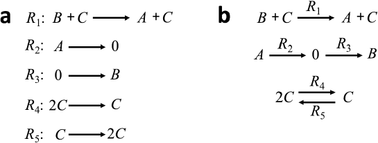
Figure 1: A simple example of a chemical reaction network (CRN). a The CRN has three species ($A,B,$ and $C$), seven complexes ($B+C$, $A+C$, $A$, $0$, $B$, $2C$, and $C$) and five reactions ($R_{1}$, $R_{2}$, $R_{3}$, $R_{4}$, and $R_{5}$). b The representation of the CRN where the reactions are grouped according to respective linkage classes.

From a dynamical perspective of a CRN, the concentrations of the species could vary when a reaction $y\to y^{\prime}$ occurs at a certain time. The change can be quantified by the difference $y^{\prime}-y$, which is called the reaction vector of $y\to y^{\prime}$. All the changes caused by the reactions belong to the subspace of the ambient space $\mathbb{R}^{m}$, known as the stoichiometric subspace of a CRN defined in the following manner

$$S:={\rm span}\left\{{y^{\prime}-y|y\to y^{\prime}\in\mathscr{R}}\right\}.$$

The $m\times r$ matrix where the $i$-th column contains the coefficients of the associated species in the $i$-th reaction vector is called the stoichiometric matrix.

Consequently, we now introduce an important concept in the theory of reaction networks, which measures the amount of linear dependency of the reactions in a CRN:

Definition 2

The deficiency of a CRN is $\delta=n-\ell-s$ where $n$ is the number of complexes, $\ell$ is the number of linkage classes, and $s$ is the dimension of the stoichiometric subspace (or the rank of the stoichiometric matrix).

Example 2

Reconsider the CRN in Example 1. The associated reaction vector to a reaction in the CRN can be obtained by subtracting the product complex by the reactant complex. For instance, associated reaction vector with the first reaction $B+C\to A+C$ can be obtained by subtracting $A+C$ (product complex) by $B+C$ (source complex). Hence, the first reaction vector is $(A+C)-(B+C)=A-B$. By associating species $A$, $B$, and $C$ to the standard basis vectors of the Euclidean space $\mathbb{R}^{3}$ (three corresponds to the number of species), $A-B=1A-1B+0C=1\cdot[1,0,0]^{\top}-1\cdot[0,1,0]^{\top}+0\cdot[0,0,1]^{\top}=[1,-1,0]^{\top}$. This is precisely the first column of the stoichiometric matrix of the CRN. The same procedure is done to obtain all the reaction vectors, and hence, all the columns of the stoichiometric matrix. The rank of this stoichiometric matrix is three ($s=3$) as inspected in Fig. 2 (right). Furthermore, by looking at Fig. 1b, there are seven complexes ($n=7$) and three linkage classes ($\ell=3$). Thus, the deficiency is $\delta=n-\ell-s=7-3-3=1$.

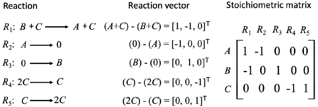
Figure 2: The stoichiometric matrix of the simple CRN in Fig. 1. A reaction vector is obtained by subtracting the product complex by the source complex of a reaction. After getting all the reaction vectors, the stoichiometric matrix is constructed by listing these vectors as columns by following the order of the reactions in the network.

We then associate a kinetics to a CRN to describe the dynamics of a given system. We define kinetics and consequently, a chemical reaction system in the following manner:

Definition 3

A kinetics for a reaction network $\mathcal{N}=(\mathcal{S},\mathcal{C},\mathcal{R})$ is an assignment to each reaction $y\to y^{\prime}\in\mathcal{R}$ of a continuously differentiable rate function $\mathcal{K}_{y\to y^{\prime}}:\mathbb{R}^{\mathcal{S}}_{>0}\to\mathbb{R}_{\geq 0}$ such that the following positivity condition holds: $\mathcal{K}_{y\to y^{\prime}}(c)>0$ if and only if ${\rm{supp\ }}y\subset{\rm{supp\ }}c$, where ${\rm{supp\ }}y$ refers to the support of the vector $y$. The system $\left(\mathcal{N},\mathcal{K}\right)$ is called a chemical kinetic system or a chemical reaction system.

Definition 4

The species formation rate function of a chemical reaction system $(\mathcal{N},\mathcal{K})$ is defined as $f\left(x\right)=\displaystyle\sum\limits_{{y}\to{y^{\prime}}\in\mathcal{R}}{{\mathcal{K}_{{y}\to{y^{\prime}}}}\left(x\right)\left({{y^{\prime}}-{y}}\right)}.$

The system of ordinary differential equations (ODEs) of a chemical reaction system is given by $\dfrac{{dx}}{{dt}}=f\left(x\right)$. In addition, a steady state or an equilibrium of the system is a vector of concentration of species that makes $f$ the zero vector. The set of positive steady states of the network $\mathcal{N}$ with specified kinetics $\mathcal{K}$ is denoted by $E_{+}:=E_{+}(\mathcal{N},\mathcal{K}).$

Definition 5

A kinetics for a CRN $(\mathcal{S},\mathcal{C},\mathcal{R})$ is mass-action if for each reaction $y\to y^{\prime}$ (i.e., $[y_{1},y_{2},\ldots,y_{m}]^{\top}\to[y_{1}^{\prime},y_{2}^{\prime},\ldots,y_{m}^{\prime}]^{\top}$),

$$\mathcal{K}_{y\to y^{\prime}}(x)=k_{y\to y^{\prime}}\prod_{i\in\mathcal{S}}x_{i}^{y_{i}}$$

for some $k_{y\to y^{\prime}}>0$.

For instance, suppose a CRN that follows the mass-action kinetics has a reaction $A+B\to B$. Then, the associated kinetics (or rate law) for the reaction is $kab$, i.e., a product of the concentrations $a$ and $b$ of species $A$ and $B$, respectively (determined by the source complex $A+B$) multiplied by the rate constant $k$.

A mass-action system is a CRN endowed with mass-action kinetics. If at least one reaction does not follow the mass-action rate function, then the system is non-mass-action. For instance, if the rate function of a certain reaction in a network follows a quotient rate law, then the corresponding system is not a mass-action system.

Example 3

Reconsider the CRN presented in Examples 1 and 2. Fig. 3 shows how to get the ODEs of a simple CRN under the mass-action kinetics. The concentrations of the species $A$, $B$, and $C$ are denoted by $a$, $b$, and $c$, respectively. To get the rate function for reaction $R_{1}:B+C\to A+C$, we multiply the concentrations of the species present in the source complex, i.e., $bc$. We then multiply it to the rate constant $k_{1}$ that we associate to reaction $R_{1}$. Thus, the rate function for the first reaction is $k_{1}bc$. A similar procedure can be followed to get the rate functions of the remaining reactions (i.e., $R_{2},\ldots,R_{5}$).

To get the ODEs associated to the CRN under the mass-action kinetics, we multiply the reaction rate with the reaction vector, e.g., $k_{1}bc\cdot[1,-1,0]^{\top}$. We do this for each reaction and get the sum over all these reactions. We then equate the result to the vector of time derivatives of the concentrations of the species (Fig. 3 bottom). Simplifying the system gives

$$\dfrac{da}{dt}= k_{1}bc-k_{2}a$$

$$\dfrac{db}{dt}= -k_{1}bc+k_{3}$$

$$\dfrac{dc}{dt}= -k_{4}c^{2}+k_{5}c.$$

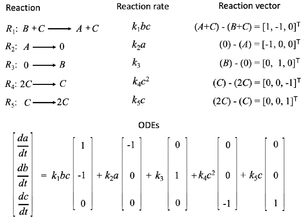
Figure 3: The ODEs of a CRN (in Fig. 1) with mass-action kinetics. Assume that the CRN follows the mass-action kinetics. To obtain the ODEs, we need to compute the reaction rate and the reaction vector for each reaction. The left-hand side of the ODEs is composed of the time derivatives of the concentration of the species. On the other hand, to get the right-hand side of the ODEs, multiply the reaction vector by the associated reaction rate of each reaction. Then, get the sum of all these products over all the reactions.

2.3 Decomposition of chemical reaction networks

We start this section with our formal definitions of a general decomposition for reaction networks (Appendix 6.A FeinbergBook2019 , Section 5.4 Feinberg1987stability ).

Definition 6

Let $\mathcal{N}$ be a reaction network and $\mathcal{R}$ be its reaction set. A decomposition of the reaction network into $\mathcal{N}_{1}$, $\mathcal{N}_{2}$, …, $\mathcal{N}_{\alpha}$ is induced by a partition of $\mathcal{R}$ into $\mathcal{R}_{1},\mathcal{R}_{2},\ldots,\mathcal{R}_{\alpha}$, respectively. The resulting networks $\mathcal{N}_{1}$, $\mathcal{N}_{2}$, …, $\mathcal{N}_{\alpha}$ are called subnetworks of $\mathcal{N}$.

Technically, we consider each $\mathcal{N}_{i}$ to have the same set of species as $\mathcal{N}$ although some of the species seem to have no role or absent in this particular subnetwork. In addition, we regard $\mathcal{N}_{i}=(\mathcal{S},\mathcal{C}_{i},\mathcal{R}_{i})$ where $\mathcal{C}_{i}$ is the set of all complexes that appear as a product or a reactant of a reaction in subnetwork $i$ FeinbergBook2019 . If $\mathcal{N}$ has only one subnetwork under the decomposition, we say that it has the trivial decomposition. This means that in this case, $\alpha=1$ and the whole network itself is the only subnetwork.

We note that each subnetwork $\mathcal{N}_{i}$ has its own stoichiometric subspace $S_{i}\subseteq S$. We are then ready to define the following concept of independent decomposition:

Definition 7

A network decomposition is said to be independent if the stoichiometric subspace of the whole network is equal to the direct sum of the stoichiometric subspaces of the subnetworks.

An equivalent way of showing independence of a CRN decomposition is to show that the rank of the stoichiometric matrix is equal to the sum of the ranks of the stoichiometric matrices of the subnetworks. In this work, we focus on the independent decomposition because of the following result by Martin Feinberg Feinberg1987stability ; FeinbergBook2019 :

Theorem 2.1

Let $\mathcal{N}$ be a CRN (with kinetics $\mathcal{K}$) decomposed into subnetworks $\mathcal{N}_{1},\mathcal{N}_{2},$ $\ldots,\mathcal{N}_{\alpha}$. Furthermore, let $\mathcal{K}_{1},\mathcal{K}_{2},\ldots,\mathcal{K}_{\alpha}$ be the restriction of $\mathcal{K}$ to reactions in $\mathcal{N}_{1},\mathcal{N}_{2},\ldots,\mathcal{N}_{\alpha}$, respectively. Then

$$E_{+}^{1}\cap E_{+}^{2}\ldots\cap E_{+}^{\alpha}\subseteq E_{+}$$

where $E_{+}^{i}$ is the set of positive steady states of subnetwork $i$. If the network decomposition is independent, then equality holds, i.e.,

$$E_{+}^{1}\cap E_{+}^{2}\ldots\cap E_{+}^{\alpha}=E_{+}.$$

Hernandez et al. Hernandezetal2022 ; HDLC2021 developed an efficient method of finding the finest independent decomposition, i.e., independent decomposition with the highest number of subnetworks. Additionally, programs built in Octave and MATLAB were created by P. Lubenia so that one can easily get the finest independent decomposition by providing the reactions of the given network LubeniaINDECS .

2.4 Generalized chemical reaction networks

We discuss the notion of generalized chemical reaction networks (GCRNs) developed by Stefan Müller and Georg Regensburger Muller2012 ; Muller2014 . Suppose that $G$ is a directed graph with vertex set $V$ and edge set $E\subseteq V\times V$. In an edge $i\to j:=(i,j)$, $i$ is called the source vertex. Denote by $V_{s}$ the set of all the source vertices in $V$. We formally define a GCRN as a directed graph $G$, with vertex set $V$, together with two maps: (i.) $y:V\to\mathbb{R}^{m}_{\geq 0}$ that assigns to each vertex a stoichiometric complex, and (ii.) $\widetilde{y}:V_{s}\to\mathbb{R}^{m}_{\geq 0}$ that assigns to each vertex a kinetic complex.

We also introduce the concept of network translation by Matthew Johnston Johnston2014 . A GCRN $\mathcal{N}^{\prime}$ is said to be a network translation of a CRN $\mathcal{N}$ if the reaction vectors of the original reactions are preserved, and the original source complexes of $\mathcal{N}$ are transferred as the kinetic complexes in $\mathcal{N}^{\prime}$ Johnston2014 ; JMP2019:parametrization . The generalized network $\mathcal{N}^{\prime}$ is also called a translated network. Hence, the original CRN $\mathcal{N}$ and the translated network $\mathcal{N}^{\prime}$ have the set of same ODEs, i.e., they are dynamically equivalent.

For instance, suppose a network $\mathcal{N}_{E}$ has only one reaction $A\to 2A$. We form $\mathcal{N}_{E}^{\prime}$ by replacing the original reaction by $0\to A$ with the same reaction vector as the original one, i.e., $A-0=2A-A$. In addition, we consider the original source complex ($A$) of the original reaction $A\to 2A$ to dictate the rate function ($ka$) to maintain the dynamics. Thus, the translated network $\mathcal{N}_{E}$ is dynamically equivalent to $\mathcal{N}_{E}^{\prime}$.

As a result, a translated network is a GCRN with two associated structures: the stoichiometric CRN and the kinetic-order CRN. The deficiencies of the stoichiometric and kinetic-order CRNs are called effective deficiency and kinetic deficiency, respectively.

In a GCRN, phantom edges are those that connect the same stoichiometric complexes. On the other hand, effective edges are those that connect different stoichiometric complexes. We denote by $E^{0}$ and $E^{*}$ the sets of phantom edges and effective edges in the GCRN, respectively. The reaction vector associated to a phantom edge is zero since this edge connects the same stoichiometric complexes. Thus, phantom edges do not contribute to the ODEs of the system. The associated dummy rate constants to these edges are considered free parameters and form a vector denoted by $\sigma$. Furthermore, we denote by $k^{*}$ the vector of rate constants associated to the effective edges.

We need one more concept to state the theorem of parametrization of positive steady states JMP2019:parametrization . This concept is the “$V^{\star}$-directed networks.” Here, we form equivalence classes such that each class contains the vertices with identical stoichiometric complex. Then, a representative is chosen for each class. In a “$V^{\star}$-directed network”, each effective edge $i\to j$ enters at a representative. In other words, the product node $j$ is associated to a representative vertex. In addition, a phantom edge starts from a representative vertex and then enter other vertex within the class. The reader can check JMP2019:parametrization for more details.

We now introduce the following main result in the paper JMP2019:parametrization of Johnston et al.

Theorem 2.2

Consider a translated network that is weakly reversible and $V^{\star}$-directed. Let $\mathcal{F}$ be any spanning forest that containing all the nodes of its kinetic-order CRN. Moreover, let $M$ be the matrix containing all the kinetic differences as rows where the entries per row are arranged according to the order of the species. Furthermore, let $H$ be a matrix such that $MHM=M$, i.e., a generalized inverse of $M$. Finally, define $B$ such that ${\rm im\ }B=\ker M$ and $\ker B=\{\mathbf{0}\}$.Then, if both the effective deficiency and the kinetic deficiency are zero, it follows that the set of positive steady states of the original network is equal to:

$${\left\{\kappa(k^{*},\sigma)^{H^{\top}}\circ\tau^{B^{\top}}|\sigma\in\mathbb{R}^{E^{0}}_{>0},\,\tau\in\mathbb{R}^{m-\tilde{s}}_{>0}\right\}\neq\varnothing}$$

where $\kappa(k^{*},\sigma)^{H^{\top}}\circ\tau^{B^{\top}}$ is the Hadamard product with the component of $\kappa$ associated with the edge $i\to i^{\prime}$ as $\kappa_{i\to i^{\prime}}=\dfrac{K_{i^{\prime}}}{K_{i}}$ and tree constant $K_{i}$ as the sum (over all the spanning trees of the kinetic-order CRN towards node $i$) of the products of the rate constants associated with the edges of each spanning tree.

2.5 Previous works and relation to the current work

Recently, Hernandez et al. Hernandez2023 proposed a framework to efficiently parametrize positive steady states of chemical reaction networks, with mass-action kinetics, that has a non-trivial independent decomposition. This approach was illustrated to be useful for power-law systems Hernandez2023powerlaw , a larger class of kinetic systems containing the mass-action.

In particular, from Theorem 2.1, the positive steady states of a given network is the intersection of the sets of positive steady states of its subnetworks when the underlying decomposition is independent. This result allowed Hernandez et al. Hernandez2023 and Hernandez and Buendicho Hernandez2023powerlaw to perform the parametrization of positive steady states of Johnston et al. JMP2019:parametrization for each of the subnetworks (endowed with mass-action kinetics and power-law kinetics, respectively) and then combining all the results to obtain the positive steady states of the original network.

Here in our current work, we consider networks that follow kinetics outside the previously considered kinetics (i.e., mass-action and power-law). For instance, we consider the case when reactions have different kinetics, e.g., some reactions follow the mass-action rate law while others follow a certain quotient rate law.

3 Results

Specifically, we propose the following general step-by-step procedure as follows:

1. Decompose the given CRN into independent subnetworks.

2. For each subnetwork, either

   1. use the method of Johnston et al. (Theorem 2.2) if it follows mass-action kinetics or power-law, or

   2. compute the positive steady states directly from the ODEs or find a transformation to mass-action system (if it exists), otherwise.

3. Combine the positive steady states of the subnetworks to get the positive steady states of the whole network.

The difference of our current approach from the previous works Hernandez2023 ; Hernandez2023powerlaw is the second step. The previous approach uses the method of Johnston et al. to all subnetworks because each subnetwork follows the mass-action or power-law kinetics. Here, we use the method of Johnston et al. for subnetworks with mass-action (or power-law) but for those that follow non-mass action (or non-power-law) kinetics such as quotient kinetics, we either compute the steady states directly from the ODEs or find a transformation to mass-action system, if it exists. We illustrate the former using a complex mathematical network of an insulin signaling pathway that involves reactions with non-mass action rate laws.

3.1 Computation of positive steady states of a complex insulin signaling pathway network with mixed kinetics via network decomposition

We illustrate our proposed method by solving the positive steady state parametrization of a complex mathematical model of insulin signaling pathway in type 2 diabetes BrannmarkInsulin2013 . The CRN of model has 36 reactions and 27 species. We let $k_{i}$ be the rate constant of reaction $R_{i}$. Furthermore, let $x_{j}$ be the concentration of species $X_{j}$. The list of reactions (left) with the associated rate laws (right) are given as follows:

$$R_{1} :X_{2}\to X_{3} k_{1}x_{2}$$

$$R_{2} :X_{2}\to X_{4} k_{2}x_{2}$$

$$R_{3} :X_{3}\to X_{4} k_{3}x_{3}$$

$$R_{4} :X_{4}\to X_{7} k_{4}x_{4}$$

$$R_{5} :X_{7}+X_{25}\to X_{6}+X_{25} k_{5}x_{7}x_{25}$$

$$R_{6} :X_{4}\to X_{2} k_{6}x_{4}$$

$$R_{7} :X_{6}\to X_{2} k_{7}x_{6}$$

$$R_{8} :X_{7}+X_{9}\to X_{7}+X_{10} k_{8}x_{7}x_{9}$$

$$R_{9} :X_{10}\to X_{9} k_{9}x_{10}$$

$$R_{10} :X_{10}+X_{31}\to X_{22}+X_{31} k_{10}x_{10}x_{31}$$

$$R_{11} :X_{22}\to X_{10} k_{11}x_{22}$$

$$R_{12} :X_{22}\to X_{33} k_{12}x_{22}$$

$$R_{13} :X_{9}\to X_{23} k_{13}x_{9}$$

$$R_{14} :X_{23}\to X_{9} k_{14}x_{23}$$

$$R_{15} :X_{10}+X_{24}\to X_{10}+X_{25} k_{15}x_{10}x_{24}$$

$$R_{16} :X_{25}\to X_{24} k_{16}x_{25}$$

$$R_{17} :X_{10}+X_{26}\to X_{10}+X_{27} k_{17}x_{10}x_{26}$$

$$R_{18} :X_{27}\to X_{26} k_{18}x_{27}$$

$$R_{19} :X_{27}+X_{33}\to X_{29}+X_{33} k_{19}x_{27}x_{33}$$

$$R_{20} :X_{22}+X_{28}\to X_{22}+X_{29} k_{20}x_{22}x_{28}$$

$$R_{21} :X_{29}\to X_{28} k_{21}x_{29}$$

$$R_{22} :X_{28}\to X_{26} k_{22}x_{28}$$

$$R_{23} :X_{29}+X_{30}\to X_{29}+X_{31} k_{23}x_{29}x_{30}$$

$$R_{24} :X_{27}+X_{30}\to X_{27}+X_{31} k_{24}x_{27}x_{30}$$

$$R_{25} :X_{31}\to X_{30} k_{25}x_{31}$$

$$R_{26} :X_{7}+X_{32}\to X_{7}+X_{33} k_{26}x_{7}x_{32}$$

$$R_{27} :X_{33}\to X_{32} k_{27}x_{33}$$

$$R_{28} :X_{29}+X_{34}\to X_{29}+X_{35} k_{28}k_{29}x_{34}$$

$$R_{29} :X_{28}+X_{34}\to X_{28}+X_{35} k_{29}\dfrac{x_{28}^{\alpha}}{\bar{k}^{\alpha}+x_{28}^{\alpha}}x_{34}$$

$$R_{30} :X_{35}\to X_{34} k_{30}x_{35}$$

$$R_{31} :X_{35}+X_{20}\to X_{35}+X_{21} k_{31}x_{35}x_{20}$$

$$R_{32} :X_{21}\to X_{20} k_{32}x_{21}$$

$$R_{33} :X_{31}+X_{36}\to X_{31}+X_{37} k_{33}\dfrac{x_{31}^{\beta}}{\tilde{k}^{\beta}+x_{31}^{\alpha}}x_{36}$$

$$R_{34} :X_{37}\to X_{36} k_{34}x_{37}$$

$$R_{35} :X_{39}\to X_{38} k_{35}x_{39}$$

$$R_{36} :X_{37}+X_{38}\to X_{37}+X_{39} k_{36}x_{37}x_{38}$$

Among the reactions in the network, only two of them (i.e., $R_{29}$ and $R_{33}$) follow non-mass-action kinetics (i.e., quotient kinetics), while the rest follow mass-action kinetics. Hence, the network follows mixed kinetics, which is a combination of mass-action and quotient rate laws.

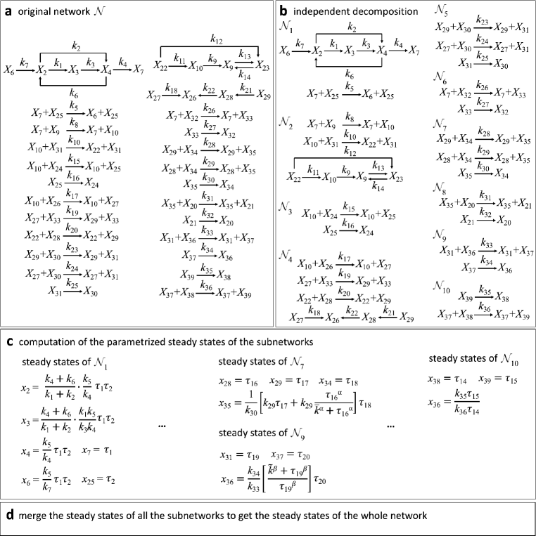
Figure 4: Parametrization of positive steady states of chemical reaction networks with mixed kinetics. a A CRN $\mathcal{N}$ of positive steady states of a complex mathematical model of insulin signaling pathway in type 2 diabetes. b $\mathcal{N}$ is decomposed into 10 independent subnetworks $\mathcal{N}_{1}\ldots\mathcal{N}_{10}$. Here, all the subnetworks except $\mathcal{N}_{7}$ and $\mathcal{N}_{9}$ follow the mass-action kinetics. On the other hand, subnetworks $\mathcal{N}_{7}$ and $\mathcal{N}_{9}$ involve reactions that follow a quotient rate function. c The steady state parametrization is computed for each subnetwork. For subnetworks $\mathcal{N}_{1}\ldots\mathcal{N}_{6},\mathcal{N}_{8},\mathcal{N}_{10}$, the parametrization process for mass-action is employed. In particular, we illustrate this process via subnetwork $\mathcal{N}_{4}$ in Fig. 5. For subnetworks $\mathcal{N}_{7}$ and $\mathcal{N}_{9}$ with just three and two reactions, respectively, the steady states are computed using elementary way of solving equations. d The steady states of the all subnetworks are merged to get the steady states of the whole network.

We solve the positive steady states of the network by following the step-by-step procedure that we have introduced in the beginning of Section 3. By applying Step S1, we decompose the network into independent subnetworks (Figure 4b). To easily get the finest independent decomposition (i.e., independent decomposition with the maximum number of subnetworks), we use the MATLAB program in LubeniaINDECS . In particular, we enter all the reactions in the network (i.e., $R_{1}$ to $R_{36}$) and run the program to output the independent decomposition.

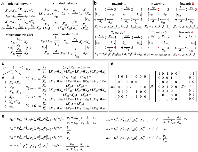
Figure 5: Parametrization of positive steady states via network translation. a The original CRN (upper left) is translated to a dynamically equivalent weakly reversible generalized network (upper right). The translated network has two substructures: the stoichiometric CRN (lower left) and the kinetic-order CRN (lower right). If the deficiencies of the stoichiometric and kinetic-order CRNs are both zero, proceed with parametrization of steady states. b Get all the spanning trees towards each node of the kinetic-order CRN where the kinetic complexes $X_{10}+X_{26}$, $X_{27}$, $X_{27}+X_{33}$, $X_{29}$, $X_{22}+X_{28}$ and $X_{28}$ are labeled by 1, 2, 3, 4, 5, and 6, respectively. Compute the tree constant $K_{i}$ by multiplying the rate constants associated to the edges of a spanning tree. Then, get the sum of the products over all the spanning trees towards complex node $i$. c Choose an arbitrary tree containing all the nodes of the kinetic-order CRN (left). Compute $\kappa_{i\to i^{\prime}}=\dfrac{K_{i^{\prime}}}{K_{i}}$, i.e., the quotient between the tree constants directed towards $i^{\prime}$ and $i$ (middle). Additionally, get the difference between the kinetic nodes associated to each edge (right). d Construct matrix $M$ such that the rows are the coefficients in the kinetic differences, $H$ is a generalized inverse of $M$ ($MHM=M$) and the ${\rm ker\ }M=B$. e Compute the parametrized steady states using the ratio of tree constants, and matrices $H$ and $B$. Here, two parameters $\tau_{1}$ and $\tau_{2}$ are introduced because there are two columns of $B$.

Then, we compute the positive steady states of each subnetwork (Step S2). Among the 10 subnetworks, eight of them ($\mathcal{N}_{1}\ldots\mathcal{N}_{6},\mathcal{N}_{8}$, and $\mathcal{N}_{10}$) follow entirely the mas-action law. Hence, the parametrization method for mass-action is employed (Step S2a). Specifically, we illustrate the method for subnetwork $\mathcal{N}_{4}$ (Figure 5).

From Theorem 2.2, we determine a translated network that is both weakly reversible and $V^{\star}$-directed (Figure 5a upper right). The translated network has effective and kinetic deficiency of zero, and hence the positive steady state can be easily parametrized (see Theorem 2.2) as described in Figure 5.

On the other hand, the remaining two subnetworks ($\mathcal{N}_{7}$ and $\mathcal{N}_{9}$) follow mixed kinetics. In particular the reactions $R_{29}$ and $R_{33}$ that follow quotient kinetics belong to subnetworks $\mathcal{N}_{7}$ and $\mathcal{N}_{9}$, respectively. In this case, the positive steady states are computed manually (Step S2b). Finally, the positive steady states of the whole network is derived by merging the positive steady states of the subnetworks (Step S3). In particular, if two subnetworks have the same species then there are two expressions for the steady state formula of such species. We equate these expressions so that we may reduce parameters and for the steady state formula to agree with both the two subnetworks.

The steady state parametrization is given as follows:

$$x_{2} =\dfrac{k_{4}+k_{6}}{k_{1}+k_{2}}\cdot\dfrac{k_{5}k_{13}}{k_{4}}\cdot\frac{\tau_{2}}{\sigma_{2}}$$

$$x_{3} =\dfrac{k_{4}+k_{6}}{k_{1}+k_{2}}\cdot\dfrac{k_{1}k_{5}k_{13}}{k_{3}k_{4}}\cdot\frac{\tau_{2}}{\sigma_{2}}$$

$$x_{4} =\dfrac{k_{5}k_{13}}{k_{4}}\cdot\dfrac{\tau_{2}}{\sigma_{2}}$$

$$x_{6} =\dfrac{k_{5}k_{13}}{k_{7}}\cdot\dfrac{\tau_{2}}{\sigma_{2}}$$

$$x_{7} =\dfrac{k_{13}}{\sigma_{2}}$$

$$x_{9} =(\sigma_{1}+k_{9})\cdot\dfrac{k_{12}k_{22}}{k_{8}k_{13}}\cdot\dfrac{\sigma_{2}}{\sigma_{1}\sigma_{4}}$$

$$x_{10} =\dfrac{k_{12}k_{22}}{\sigma_{1}\sigma_{4}}$$

$$x_{20} =\dfrac{k_{32}}{k_{31}}\cdot\dfrac{\tau_{12}}{\tau_{13}}$$

$$x_{21} =\tau_{12}$$

$$x_{22} =\dfrac{k_{22}}{\sigma_{4}}$$

$$x_{23} =\dfrac{k_{12}k_{22}}{k_{8}k_{14}}\cdot\dfrac{\sigma_{1}\sigma_{2}+\sigma_{1}k_{8}+\sigma_{2}k_{9}}{\sigma_{1}\sigma_{4}}$$

$$x_{24} =\dfrac{k_{16}}{k_{15}}\cdot\dfrac{\tau_{2}}{x_{10}}$$

$$x_{25} =\tau_{2}$$

$$x_{26} =\dfrac{\sigma_{3}+k_{18}}{(\sigma_{4}+k_{20})(\sigma_{5}+k_{23})}\cdot\dfrac{k_{21}k_{25}}{k_{12}k_{17}k_{22}}\cdot\dfrac{\sigma_{1}\sigma_{4}^{2}}{\sigma_{3}}\cdot\dfrac{\tau_{9}}{\tau_{8}}$$

$$x_{27} =\dfrac{\sigma_{5}}{k_{23}+\sigma_{5}}\cdot\dfrac{k_{25}}{k_{24}}\cdot\dfrac{\tau_{9}}{\tau_{8}}$$

$$x_{28} =\dfrac{\sigma_{4}}{(\sigma_{4}+k_{20})(\sigma_{5}+k_{23})}\cdot\dfrac{k_{21}k_{25}}{k_{22}}\cdot\dfrac{\tau_{9}}{\tau_{8}}$$

$$x_{29} =\dfrac{k_{25}}{\sigma_{5}+k_{23}}\cdot\dfrac{\tau_{9}}{\tau_{8}}$$

$$x_{30} =\tau_{8}$$

$$x_{31} =\tau_{9}$$

$$x_{32} =\dfrac{k_{27}\sigma_{2}\sigma_{3}}{k_{13}k_{19}k_{26}}$$

$$x_{33} =\dfrac{\sigma_{3}}{k_{19}}$$

$$x_{34} =\tau_{18}$$

$$x_{35} =\dfrac{\tau_{18}}{k_{30}}\left[k_{28}\tau_{7}+k_{29}\cdot\dfrac{x_{28}^{\alpha}}{\bar{k}^{\alpha}+x_{28}^{\alpha}}\right]$$

$$x_{36} =\dfrac{k_{34}k_{35}}{k_{33}k_{36}}\cdot\dfrac{\tilde{k}^{\beta}+x_{31}^{\beta}}{x_{31}^{\beta}}\cdot\dfrac{\tau_{15}}{\tau_{14}}$$

$$x_{37} =\dfrac{k_{35}}{k_{36}}\cdot\dfrac{\tau_{15}}{\tau_{14}}$$

$$x_{38} =\tau_{14}$$

$$x_{39} =\tau_{15}$$

where

$$\sigma_{5} =\dfrac{\sigma_{4}k_{21}k_{24}}{(\sigma_{4}+k_{20})\sigma_{3}}$$

$$\tau_{9} =\dfrac{k_{11}+k_{12}}{k_{10}k_{12}}\cdot\sigma_{1}$$

$$\tau_{7} =\dfrac{k_{25}}{\sigma_{5}+k_{23}}\cdot\dfrac{\tau_{9}}{\tau_{8}}$$

$$\tau_{16} =\dfrac{\sigma_{4}k_{21}k_{25}}{\sigma_{3}(\sigma_{3}+k_{20})(\sigma_{5}+k_{23})}\cdot\dfrac{\tau_{7}\tau_{9}}{\tau_{8}}$$

$$\tau_{13} =\dfrac{\tau_{18}}{k_{30}}\cdot\left[k_{28}\tau_{7}+k_{29}\cdot\dfrac{\tau_{16}^{\alpha}}{\bar{k}^{\alpha}+\tau_{16}^{\alpha}}\right]$$

and $\tau_{2},\tau_{8},\tau_{9},\tau_{12},\tau_{14},\tau_{15},\tau_{18},\sigma_{1},\sigma_{2},\sigma_{3},\sigma_{4}>0$.

Using the obtained parametrization, we can easily identify if the given system has absolute concentration robustness (ACR) in a particular species. The ACR is a concept introduced by Guy Shinar and Martin Feinberg ShinarFeinberg2010 in the journal Science in 2010. A system with ACR at a particular species maintains the steady state concentration of the species at a constant level despite environmental fluctuations.

As we can inspect from the steady state formulas $x_{i}$ of species $X_{i}$, the system has no ACR in all the species because each steady state value depends on some free parameters. For instance, $x_{2}$ depends on both $\tau_{2}$ and $\sigma_{2}$. Similarly, $x_{31}$ depends on $\tau_{9}$ while $\tau_{9}$ depends on $\sigma_{1}>0$. Note that specific values for the free parameters can be solved by using the conservation laws.

4 Computation of positive steady states via a transformation of an associated system to mass-action

This section was motivated by the following interesting example from Yu and Craciun Yu2018 . The CRN $\mathcal{N}$ with two reactions together with their associated rate functions:

$$R_{1}:X_{1}+X_{2}\to 2X_{1} \dfrac{k_{1}x_{1}x_{2}}{k_{2}+x_{1}}$$ (1)

$$R_{2}:2X_{2}\to X_{1}+X_{2} k_{3}x_{1}^{2}.$$ (2)

The first reaction $R_{1}$ follows a rational reaction rate function (i.e., Michaelis-Menten rate function) while the second one follows $R_{2}$ the standard mass-action rate function. Because $R_{1}$ and $R_{2}$ have different reaction rate functions, i.e., Michaelis-Menten and mass-action, we say that the CRN follows mixed kinetics. The associated system of ordinary differential equations (ODEs) for the CRN under the specified mixed kinetics is

$$\dfrac{dx_{1}}{dt} =\dfrac{k_{1}x_{1}x_{2}}{k_{2}+x_{1}}-k_{3}x_{1}^{2}$$ (3)

$$\dfrac{dx_{2}}{dt} =-\dfrac{k_{1}x_{1}x_{2}}{k_{2}+x_{1}}+k_{3}x_{1}^{2}.$$ (4)

According to Yu and Craciun Yu2018 , may can study the following system of ODEs:

$$\dfrac{dx_{1}}{dt} =k_{1}x_{1}x_{2}-k_{2}k_{3}x_{1}^{2}-k_{3}x_{1}^{3}$$ (5)

$$\dfrac{dx_{2}}{dt} =-k_{1}x_{1}x_{2}+k_{2}k_{3}x_{1}^{2}+k_{3}x_{1}^{3}$$ (6)

instead of the system of ODEs composed of Equations 3 and 4. The associated CRN $\mathcal{N}^{\prime}$, identified by its reactions and their rate functions, to the system of ODEs are given as follows:

$$R_{1}:X_{1}+X_{2}\to 2X_{1} k_{1}x_{1}x_{2}$$ (7)

$$R_{2}:2X_{1}\to X_{1}+X_{2} k_{2}^{\prime}x_{1}^{2}$$ (8)

$$R_{3}:3X_{1}\to 2X_{1}+X_{2} k_{3}x_{1}^{3}$$ (9)

Note that when we multiply the ODEs associated to the mixed kinetics, by $k_{2}+x_{1}$, we precisely get the ODEs associated to the mass-action kinetics where $k_{2}^{\prime}=k_{2}k_{3}$.

COMPILES (COMPutIng anaLytic stEady States) is a computational package Hernandez2023 built in MATLAB to compute analytic positive steady states of a mass-action system and is available at https://github.com/Mathbiomed/COMPILES. A user inputs all the reactions in a given network and outputs the positive steady state parametrization of the network under mass-action kinetics. By entering Equations 7, 8, and 9, we obtain the following parametrization:

$$x_{1}=\dfrac{\sigma}{k_{3}}\text{ and }x_{2}=\dfrac{\sigma(k_{2}^{\prime}+\sigma)}{k_{1}k_{3}}=\dfrac{\sigma(k_{2}k_{3}+\sigma)}{k_{1}k_{3}}.$$

One can easily check that the parametrization satisfies the original ODEs with Equations 3 and 4.

On the other hand, consider the following CRN with polynomial kinetics

$$R_{1}:X_{1}\to X_{2} k_{1}x_{1}$$ (10)

$$R_{2}:X_{1}+X_{2}\to 2X_{1}+2X_{2} k_{2}+k_{3}x_{2}.$$ (11)

The system given by Equations 10 and 11 has a dynamically equivalent mass-action system with the following ODEs:

$$R_{1}:X_{1}\to X_{2} k_{1}x_{1}$$

$$R_{2}:0\to X_{1}+X_{2} k_{2}$$

$$R_{3}:X_{2}\to X_{1}+2X_{2} k_{3}x_{2}.$$

This work can open a direction of studying associated ODEs in the format of mass-action. In particular, one may explore the conditions on when a given system has an associated or dynamically equivalent mass-action system. We also note that for complex networks, decomposition of the network into independent subnetworks could also be employed.

5 Summary and Outlook

We proposed a framework to derive positive steady states of chemical reaction networks with nontrivial independent decomposition that follow non-mass action kinetics, which may include polynomials, quotients, and mixed kinetics. This is done by modifying the algorithm in our previous works that focus on mass-action kinetics and power-laws Hernandez2023 ; Hernandez2023powerlaw . In particular, after decomposing a given CRN into independent subnetworks, we compute the positive steady states of subnetworks that follow purely mass-action (or power-law), while on the other hand, we manually compute the positive steady states of subnetworks that follow other types of kinetics. We illustrated this approach via a complex mathematical model of insulin signaling pathway in type 2 diabetes BrannmarkInsulin2013 . Using the obtained steady state parametrization, we were able to check the so-called absolute concentration robustness property for each species in the given network. It would be very exciting to study chemical and biological properties of important systems existing in literature using our approach. Furthermore, we have initiated to look into transformations of non-mass-action systems to mass-action. It is interesting to explore research in this direction.

Declarations

Ethical Approval. This declaration is not applicable.

Competing interests. The authors declare no competing interests.

Authors’ contributions. All authors wrote the main manuscript text. BSH prepared all the figures. All authors reviewed the manuscript.

Availability of data and materials. This declaration is not applicable.

References

- (1) Brännmark, C., Nyman, E., Fagerholm, S., Bergenholm, L., Ekstrand, E., Cedersund, G., Strålfors, P.: Insulin signaling in type 2 diabetes: experimental and modeling analyses reveal mechanisms of insulin resistance in human adipocytes. J Biol Chem 288, 9867–9880 (2013). DOI 10.1074/jbc.m112.432062
- (2) Feinberg, M.: Lectures on chemical reaction networks (1979). URL https://crnt.osu.edu/LecturesOnReactionNetworks. Written version of lectures given at the Mathematical Research Center, University of Wisconsin, Madison
- (3) Feinberg, M.: Chemical reaction network structure and the stability of complex isothermal reactors I: The deficiency zero and deficiency one theorems. Chem. Eng. Sci. 42, 2229–2268 (1987)
- (4) Feinberg, M.: Foundations of Chemical Reaction Network Theory. Springer International Publishing (2019)
- (5) Hernandez, B., Amistas, D., De la Cruz, R., Fontanil, L., de los Reyes, A., Mendoza, E.: Independent, incidence independent and weakly reversible decompositions of chemical reaction networks. MATCH Commun. Math. Comput. Chem. 87(2), 367–396 (2022)
- (6) Hernandez, B., Buendicho, K.: A network-based parametrization of positive steady states of power-law kinetic systems (2023). Submitted
- (7) Hernandez, B., De la Cruz, R.: Independent decompositions of chemical reaction networks. Bull. Math. Biol. 83(7), 76 (2021)
- (8) Hernandez, B., Lubenia, P., Johnston, M., Kim, J.K.: A framework for deriving analytic long-term behavior of biochemical reaction networks (2023). PLOS Computational Biology
- (9) Hong, H., Hernandez, B., Kim, J., Kim, J.K.: Computational translation framework identifies biochemical reaction networks with special topologies and their long-term dynamics (2023). SIAM Journal on Applied Mathematics
- (10) Johnston, M., Burton, E.: Computing weakly reversible deficiency zero network translations using elementary flux modes. Bull. Math. Biol. 81, 1613–1644 (2019)
- (11) Johnston, M.D.: Translated chemical reaction networks. Bull. Math. Biol. 76, 1081–1116 (2014)
- (12) Johnston, M.D., Müller, S., Pantea, C.: A deficiency-based approach to parametrizing positive equilibria of biochemical reaction systems. Bull. Math. Biol. 81, 1143–1172 (2019)
- (13) Lubenia, P.: INDECS: INdependent DEComposition of networkS, Available online:. https://github.com/pvnlubenia/INDECS
- (14) Müller, S., Regensburger, G.: Generalized mass action systems: Complex balancing equilibria and sign vectors of the stoichiometric and kinetic-order subspaces. SIAM J. Appl. Math. 72, 1926–1947 (2012)
- (15) Müller, S., Regensburger, G.: Generalized mass-action systems and positive solutions of polynomial equations with real and symbolic exponents (invited talk). In: V.P. Gerdt, W. Koepf, W.M. Seiler, E.V. Vorozhtsov (eds.) Computer Algebra in Scientific Computing. CASC 2014. Lecture Notes in Computer Science, vol. 8660, p. 302–323. Springer (2014)
- (16) Shinar, G., Feinberg, M.: Structural sources of robustness in biochemical reaction networks. Science 327, 1389–1391 (2010). DOI 10.1126/science.1183372
- (17) Yu, P., Craciun, G.: Mathematical analysis of chemical reaction systems. Israel Journal of Chemistry 58, 733–741 (2018)