F-12 density matrices and cumulants from the explicitly connected coupled-cluster theory

Abstract

We present the expansion to the expectation value coupled cluster theory (XCC) to the wavefunctions that include the inter electronic distances $r_{12}$ explicitly. We have extended our algebraic manipulation code Paldusto deal with the rems arising in the CC-F12 theory. We present the full working expressions for the one-electron density matrix (1RDM) and cumulant of the two-electron density matrix ($\lambda$-2RDM) in the framework of XCC-F12 theory. We analyze the computational cost and discuss the possible approximations the expressions.

1   Introduction

For the computation of the molecular properties of small- and medium-sized systems the coupled cluster (CC) theory^{1, 2, 3} is the leading ab initio approach. CC method is size extensive and allows for systematic approximation by including selected excitations. Currently CC is routinely used for the computation of ground-state energies, molecular properties, excited states, etc.

Still, to obtain chemical accuracy ($<1$ kcal mol^-1) without including costly, higher excitations, one needs to address the incompleteness of the basis set that causes the well-known basis set error. It originates from the fact that one-electron orbitals are used to construct two-electron basis sets. It was known since 1957 Kato’s discovery of the cusp condition⁴ that the inclusion of the inter electronic distance $r_{12}$ explicitly in the wave function might lead to the construction of an efficient wavefunction.

The main obstacle of using such methods are the high-dimension integrals arising in the theory. So far numerous approaches to deal with this problem have been proposed, form the direct evaluation of the high-dimension integrals^{5, 6}, through expanding the correlation factor in terms of Gaussian Geminals^{7, 8}, to the well known R12/F12 methods proposed by Kutzelnig^{9, 10} where through the insertion of the resolution of identity (RI) only two-electron integrals remain. Numerous approaches have been developed to deal with this problem. Among them the standard approximation idea (SA), proposed by Kutzelnig and Klopper, to introduce the resolution of identity (RI) to the integrals which allows for a reduction of the three- and four-electron integrals to two-electron terms.

Although the SA simplified the integrals, the $r_{12}$ methods still required to use large basis sets.^{10, 11, 12} This problem was addressed be Klopper and Samson¹³ by the introduction of ABS basis - additional basis set for the RI. Valeev¹⁴ proposed a robust modification to this approach called the complementary auxiliary basis set - CABS method which involves expansion in the orthogonal complement to the span of orbital basis set (OBS). which will be utilized in this work. The large CABS basis is used only for the RI terms and the normal orbital basis set is retained for the rest of the terms, making the $r_{12}$ methods feasible.

Within the standard approximation the CC-F12 theory was first presented by Noga and collaborators.¹⁵ The exponential form generates highly nonlinear, complicated expressions, therefore it is a common practice to further approximate the expressions for the amplitude, e.g. Fliegl^{16, 17}, Tew¹⁸ or Ten-no.¹⁹ Shiozaki²⁰ presented the full form of the CC method up to the quadruple exctitaions for ground state (CC-R12), excited states (EOM-CC-R12) and for the $\Lambda$ equation ($\Lambda$-CC-R12) of the CC analytical gradient theory.

In this work we propose introducing the explicitly correlated wavefunction to the computation of the one electron density matrix (1RDM) and the cumulant of the two-electron density matrix ($\Lambda$-2RDM) in the framework of the expectation value coupled cluster theory (XCC)^{21, 22, 23}. In this way we propose more accurate method to the computation of one- and two-electron properties of the ground state, while making use of the XCC ability of highly controllable approximations, at relatively low cost.

2   The CC-F12 theory

In the CC-F12 theory the wavefunction $\Psi_{0}$ is represented by the usual coupled cluster expansion

$$\Psi_{0}=e^{T}\Phi_{0}$$ (1)

where $\Phi_{0}$ is the reference determinant usually Hartree-Fock determinant, and the cluster operator $T$ is a sum of $n$-tuple excitation operators

$$T=\sum_{n=1}^{N}T_{n}$$ (2)

where $N$ is the number of electrons. Each of the cluster operators can be represented by the product of singlet excitation operators $E_{ai}$²⁴

$$T_{n}=\frac{1}{n!}\sum_{\mu_{n}}^{N}t_{\mu_{n}}\mu_{n}=\frac{1}{n!}\sum_{\mu_{n}}^{N}t_{\mu_{n}}E_{ai}E_{bj}\ldots E_{fm},$$ (3)

where $\mu_{n}$ denotes $n$-th excitation level. The indices $a,b,c\ldots$, $i,j,k\ldots$ and $p,q,r\ldots$ denote virtual, occupied and general orbitals, respectively,see Table LABEL:. When we restrict the excitations to single and double the cluster operator is composed of the standard part supplemented by the explicitly correlated component,

$$\begin{split}&T=T_{1}+T_{2}+T_{2}^{\prime},\\ &T_{2}^{\prime}=\frac{1}{2}\sum_{ijkl}(t_{2}^{\prime})^{kl}_{ij}\left[\sum_{\alpha\beta}\left\langle\alpha\beta\middle|\right.f_{12}\left.\middle|kl\right\rangle E_{\alpha i}E_{\beta j}\right.\\ &\left.-\sum_{ab}\left\langle ab\middle|\right.f_{12}\left.\middle|kl\right\rangle E_{ai}E_{bj}\right]\end{split}$$ (4)

where $\alpha,\beta\ldots$ denote the complete set of orbitals, $f_{12}$ is the $r_{12}$-dependent correlation factor. The new operator $T_{2}^{\prime}$ should satisfy the condition

$$T_{2}^{\prime}=\hat{Q}_{12}T_{2}^{\prime}$$ (5)

in order to assure that $T_{2}^{\prime}$ is strongly orthogonal to products of occupied orbitals. This ensures that $T_{2}$ produces only two-electron correlation effect. The $\hat{Q}_{12}$ can take several forms, among which is the so-called ansatz-3 proposed by Veleev¹⁴

$$\hat{Q}_{12}=(1-\hat{O}_{1})(1-\hat{O}_{2})-\hat{V}_{1}\hat{V}_{2}\\ =\hat{V}_{1}(1-\hat{P}_{2})+(1-\hat{P}_{1})\hat{V}_{2}+(1-\hat{P}_{1})(1-\hat{P}_{2})$$ (6)

where $\hat{O}_{i}$, $\hat{V}_{i}$ and $\hat{P}_{i}$ are the projections onto the occupied, virtual, and all orbital basis orbitals respectively, and $(1-\hat{P}_{i})$ projects on the set of virtual orbitals of the complete basis that does not include virtual orbitals from orbital basis, see Table 1 and Fig. 1. This particular form of the $\hat{Q}_{12}$ operator allows us to approximate the $(\hat{1}-\hat{P})$ subspace instead of approximating the whole space $\hat{1}$.

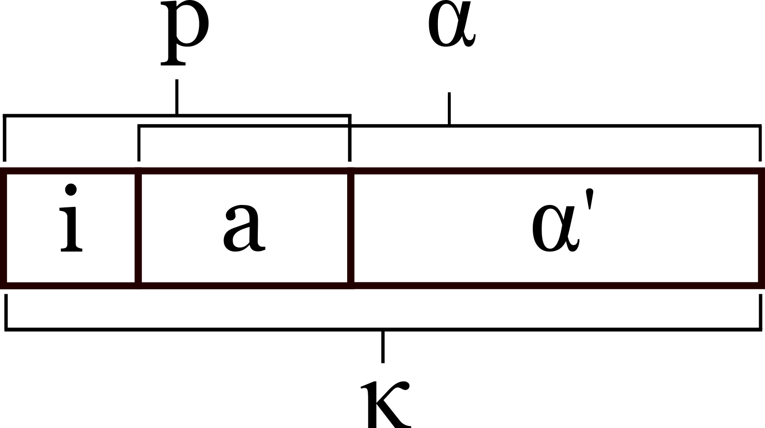
Figure 1: Partition of orbital space in CABS R12 with corresponding indices

$\hat{O}_{i}$	$i,j,k,l\ldots$	occupied
$\hat{V}_{i}$	$a,b,c,d\ldots$	virtual in OBS
$\hat{P}_{i}$	$p,q,r,s\ldots$	general in OBS
$\hat{1}$	$\kappa,\lambda,\mu,\nu\ldots$	general in complete
$\hat{1}-\hat{O}$	$\alpha,\beta,\gamma,\delta\ldots$	virtual in complete
$\hat{1}-\hat{P}$	$\alpha^{\prime},\beta^{\prime},\gamma^{\prime},\delta^{\prime}\ldots$	virtual in complete - OBS
$\hat{P}_{i}^{{}^{\prime}}$	$a^{\prime},b^{\prime},c^{\prime},d^{\prime}\ldots$	virtual in CABS

Table 1: Projectors on spaces and corresponding indices

The operator $T_{2}^{\prime}$ is a product of the geminal amplitudes $(t_{2}^{\prime})^{kl}_{ij}$ and molecular integrals $F^{\alpha\beta}_{kl}$ involving an explicit $r_{12}$ dependent factor.

$$F^{\alpha\beta}_{kl}=\int\int d\mathbf{r}_{1}d\mathbf{r}_{1}\phi_{\alpha}(\mathbf{r}_{1})^{*}$$ (7)

$$\phi_{\beta}(\mathbf{r}_{2})^{*}f_{12}(\phi_{k}(\mathbf{r}_{1})\phi_{l}(\mathbf{r}_{1})-\phi_{l}(\mathbf{r}_{1})\phi_{k}(\mathbf{r}_{1}))$$ (8)

with $\hat{P}_{1}\phi_{\alpha}=0$ or $\hat{P}_{2}\phi_{\beta}=0$, and $F^{\alpha\beta}_{kl}=0$ otherwise. For the $f_{12}$ correlation factor we used the Slater-type function of $r_{12}$

$$f_{12}=(-\gamma r_{12}).$$ (9)

The Ansatz Eq. (1), with thus defined $T$ amplitudes, Eq. (LABEL:rownanie-t), is incorporated into the Schrodinger equation

$$\hat{H}\Psi_{0}=E\Psi_{0}$$ (10)

with Hamiltonian $\hat{H}$ defined as

$$\hat{H}=\sum_{\kappa\lambda}h_{\kappa\lambda}E_{\kappa\lambda}+\frac{1}{2}\sum_{\kappa\lambda\zeta\tau}g_{\kappa\lambda\zeta\tau}E^{\kappa\lambda}_{\zeta\tau},$$ (11)

where $\kappa,\lambda,\zeta\ldots$ denote general indices in a complete basis, Table 1. The equation is then multiplied from the left by $e^{-T}$ and projected into the excited manifold producing the full CCSD-F12 expression for the energy, and CC-F12 amplitudes

$$\left\langle\Phi_{0}\middle|\right.\bar{H}\left.\middle|\Phi_{0}\right\rangle$$ (12)

$$\left\langle\Phi^{a}_{i}\middle|\right.\bar{H}\left.\middle|\Phi_{0}\right\rangle$$ (13)

$$\left\langle\Phi^{ab}_{ij}\middle|\right.\bar{H}\left.\middle|\Phi_{0}\right\rangle$$ (14)

$$\left\langle\Phi^{kl}_{ij}\middle|\right.\bar{H}\left.\middle|\Phi_{0}\right\rangle.$$ (15)

$\bar{H}$ denotes the similarity transformed Hamiltonian $e^{-T}\hat{H}e^{T}$.

3   Elimination of the complete basis set

In the CC-F12 theory, the elimination of indices $\kappa,\lambda\ldots$ which run through the complete basis set is necessary in order to obtain expressions that are computationally manageable. Table 1 and Fig. 1 summarize how the space is divided in the CABS approach, and associates the specified indices with the corresponding subspace. The choice of the operator $\hat{Q}_{12}$ allows for an efficient approximation of the special intermediates of the F12 theory

$$\begin{split}&\mathcal{V}^{pq}_{ij}=\frac{1}{2}g_{pq\alpha\beta}F^{\alpha\beta}_{ij}\\ &\mathcal{X}^{kl}_{ij}=\frac{1}{2}F_{\alpha\beta}^{kl}F^{\alpha\beta}_{ij}\\ &\mathcal{B}^{kl}_{ij}=\frac{1}{2}F_{\alpha\beta}^{kl}f_{\alpha\gamma}F^{\beta\gamma}_{ij}\\ &\mathcal{P}^{kl}_{ij}=\frac{1}{2}F_{\alpha\beta}^{kl}f_{\alpha\beta\gamma\delta}F^{\gamma\delta}_{ij}\end{split}$$ (16)

which are rewritten in terms of the products of two-electron integrals expressed in either the OBS basis or the complete basis belonging to the $\hat{1}-\hat{P}$ subspace. The complete basis is further approximated by the finite CABS basis belonging to the $\hat{P}^{{}^{\prime}}$ subspace

$$\phi_{\alpha^{\prime}}\approx\phi_{a^{\prime}}.$$ (17)

The special intermediates are identified in the orbital expressions, before any approximations take place, and are marked for an evaluation of an external integral engine during the computation stage. All other terms involving the summation over the complete basis are approximated by replacing $\alpha^{\prime}$ by $a^{\prime}$.

4   XCC approach to the computation of properties

In the literature, there are several rigorous approaches that can be extended to calculate the molecular properties of the CC-F12 theory. The first approach base on the differentiation of CC energy expressions was introduced by Monkhorst^{25, 26} in 1997 and later extended by Bartlett^{27, 28, 29} et. al. and is known as the $\Lambda$ vector technique. Koch and Jørgensen^{30, 31, 32} proposed the time-averaged quasi-energy Lagrangian technique TD-CC. In these approaches a set of linear response equations must be solved to obtain the $\Lambda$ vector. With this quantity at hand the CC expectation value can be calculated from a non-symmetric expression alike

$$\bar{X}=\braket{(1+\Lambda)e^{(-T)}Xe^{T}},$$ (18)

where $\braket{A}$ denotes the expectation value of an operator A with a reference wavefunction, $\Phi_{0}$.

The second approach called XCC theory is based on the computation of molecular properties directly from the average value of an operator^{21, 22}

$$\bar{X}=\frac{\left\langle\Psi_{0}\middle|\right.X\left.\middle|\Psi_{0}\right\rangle}{\left\langle\Psi_{0}\middle|\Psi_{0}\right\rangle}.$$ (19)

The wavefunction $\Psi_{0}$ is parameterized by the CC ansatz, and an auxiliary operator S is introduced by means of the following formula

$$e^{S}\Phi_{0}=\frac{e^{T^{\dagger}}e^{T}\Phi_{0}}{\left\langle e^{T}\middle|e^{T}\right\rangle}\qquad S=S_{1}+S_{2}+\ldots S_{N}$$ (20)

where N is the number of electrons in the system. With help of this auxiliary operator the CC expectation value is rewritten as

$$\bar{X}=\braket{e^{S^{\dagger}}e^{-T}Xe^{T}e^{-S^{\dagger}}}.$$ (21)

The average value of X can then be expressed as a finite series of commutators in this approach.

It is important to differentiate the XCC method discussed in this work from the approach developed by Bartlett and Noga with the same name.³³ Also the operator $S$ was introduced by Arponen and coworkers in the context of the extended coupled cluster theory (ECC).^{34, 35, 36} However, the $S$ operator was defined in their work by a set of nonlinear equations for which no systematic approximation scheme existed. Later, Jeziorski and Moszynski²¹ proposed an expression for $S$ that could be systematically approximated by satisfying a set of linear equations. The main finding of their work describing the $S$ operator technique is that the operator $S$ is related to the operator $T$ by means of a relatively simple linear equation. Moreover, this equation does not need to be solved in practice. In fact, the operator $S$ can be expanded in a combined power series of the cluster operators $T$ and $T^{\dagger}$,

$$S_{n}=T_{n}-\frac{1}{n}\mathcal{P}_{n}[\sum_{k=1}\sum_{p=1}\frac{1}{k!}p[T_{p}^{\dagger},T]_{k}\\ +\sum_{k=1}\sum_{m=0}\sum_{p=1}\frac{1}{k!}\frac{1}{m!}p[[S_{p},T^{\dagger}]_{k},T]_{m}]$$ (22)

and $[A,B]_{k}$ is a shorthand for a $k$-times nested commutator. The superoperator $\hat{\mathcal{P}}_{n}(X)$ yields the excitation part of $X$

$$\hat{\mathcal{P}}_{n}(X)=\frac{1}{n!}\sum_{\mu_{n}}\braket{\mu_{n}}{X}\mu_{n}.$$ (23)

where for simplicity we introduce the following notation $\braket{A}{B}=\braket{A\Phi_{0}}{B\Phi_{0}}$. It is clear from the expressions above that it can be truncated, e.g. on the basis of the perturbation theory arguments. This also constitutes the biggest advantage of the $S$ operator technique over the $\Lambda$ method. The task of solving the response equations to obtain $\Lambda$ is almost as expensive as the original CC iterations themselves. Computation of the operator $S$, on the other hand, is a relatively simple one-step (non-iterative) procedure which can be accomplished very efficiently. Since its introduction, the $S$ operator technique has been applied to calculation of the molecular properties at the conventional CCSD and CC3 levels³⁷, CC3 transition moments between the ground and excited states³⁷ and excited to excited states³⁸, electrostatic and exchange contributions to the interaction energies of closed-shell systems^{39, 22, 40} and others. The $S$ operator technique has, not yet been utilized in the context of explicitly correlated wavefunctions.

5   F-12 expressions for the Operator $\mathbf{S}$

In the explicitly correlated version of CC, the $T_{2}$ amplitudes are supplemented by the explicitly correlated component from Eq. (LABEL:rownanie-t). For the purpose of deriving expressions for the $S$ amplitudes, we rewrite the T amplitudes in a more compact form

$$\begin{split}&T_{1}=\sum_{\alpha i}t^{\alpha}_{i}h(\alpha)E_{\alpha i}\\ &T_{2}=\frac{1}{2}\sum_{\alpha\beta ij}\left(\bar{\bar{t}}^{\alpha\beta}_{ij}p(\alpha)p(\beta)+t^{\alpha\beta}_{ij}h(\alpha)h(\beta)\right)E_{\alpha i}E_{\beta j}\\ \end{split}$$ (24)

where

$$\bar{\bar{t}}^{\alpha\beta}_{ij}=\sum_{kl}(t_{2}^{{}^{\prime}})^{kl}_{ij}F^{\alpha\beta}_{kl}$$ (25)

and $h(\alpha)$ and $p(\alpha)$ are defined as

$$\begin{split}&h(\alpha)=0\quad\mbox{if}\quad\alpha\in(1-\hat{P})\\ &h(\alpha)=1\quad\mbox{if}\quad\alpha\in\hat{V}\\ &p(\alpha)=1\quad\mbox{if}\quad\alpha\in(1-\hat{P})\\ &p(\alpha)=0\quad\mbox{if}\quad\alpha\in\hat{V}.\end{split}$$ (26)

Expressing the $T$ amplitudes in a complete basis allows us to re-derive the expressions for the $S$ amplitudes starting from Eq. (20)

$$e^{T^{\dagger}}e^{T}\Phi_{0}=\left\langle e^{T}\middle|e^{T}\right\rangle\Phi_{0}.$$ (27)

We will not follow the full derivation as it can be found in the original work ²¹, instead we only note changes necessary to obtain the $S$-F12 amplitudes.

We act on both sides of Eq. (27) with the $Q$ operator expressed in the complete basis

$$Q=\alpha^{\dagger}\alpha$$ (28)

to ensure it satisfies $[Q,T_{n}]=nT_{n}$ and $[Q,S_{n}]=nS_{n}$ with the F12 amplitudes. Next we multiply both sides by $e^{-T}e^{-T^{\dagger}}e^{S}$

$$e^{-T}e^{-T^{\dagger}}e^{S}Qe^{-S}e^{T^{\dagger}}e^{T}=0.$$ (29)

In order to obtain the $S$-F12 version of the set of linear equations from Eq. (22), we project Eq. (29) onto the $n$-tuply excited states in a complete basis, to retain information on $T_{2}^{{}^{\prime}}$. Only in this way we are able to recover the first approximation to the $S$ amplitudes, which should be equal to $T_{2}+T_{2}^{{}^{\prime}}$. This implicates the form of the projection operator $\hat{\mathcal{P}}_{n}$ which spans over the complete basis, i.e.

$$\hat{\mathcal{P}}_{n}(X)=\frac{1}{n!}\sum_{\begin{subarray}{c}i_{1}\ldots i_{n}\\ \alpha_{i}\ldots\alpha_{n}\end{subarray}}\braket{\mu_{\begin{subarray}{c}i_{1}\ldots i_{n}\\ \alpha_{i}\ldots\alpha_{n}\end{subarray}}}{X}\mu_{\begin{subarray}{c}i_{1}\ldots i_{n}\\ \alpha_{i}\ldots\alpha_{n}\end{subarray}}.$$ (30)

Eq. (22) is a linear equation that can be solved iteratively but it was proven more practical to expand $S_{n}$ by either MBPT expansion or expansion in powers of $T$. In this work we obtain the $T$ amplitudes from CC-F12 theory, where we in fact perform a summation to an infinite MBPT order. However, to facilitate discussion and formula verification, one should keep in mind that the $T$ amplitudes can be expanded into MBPT orders as follows:^{41, 21}

$$\begin{split}&T_{1}^{(2)}=T_{1}^{\{2\}}+T_{1}^{\{3\}}+\ldots\\ &T_{2}^{(1)}=T_{2}^{\{1\}}+T_{2}^{\{2\}}+\ldots\end{split}$$ (31)

where the superscript in curly braces indicates the pure MBPT order and the superscript in round parentheses denotes the lowest MBPT order in which the term appears for the first time. When the $T$ amplitudes are acquired from CCSD-F12 approximation, $T=T_{1}+T_{2}+T_{2}^{\prime}$ the leading terms for the operators $S_{n}^{(m)}$ are

$$\begin{split}S_{1}^{(2)}&=T_{1}^{(2)}=T_{1}^{\{2\}}+T_{1}^{\{3\}}+\ldots\\ S_{2}^{(1)}&=T_{2}+T_{2}^{{}^{\prime}}\\ S_{1}^{(3)}&=\hat{\mathcal{P}}_{1}\left([T_{1}^{\dagger},T_{2}+T_{2}^{\prime}]\right)\\ S_{2}^{(3)}&=\frac{1}{2}\hat{\mathcal{P}}_{2}\left([[T_{2}^{\dagger}+(T_{2}^{\dagger})^{\prime},T_{2}+T_{2}^{\prime}],T_{2}+T_{2}^{\prime}]\right).\end{split}$$

We stress that because of the CCSD approximation we are not including some of the low order terms, that are expressed through $T_{3}$ or higher amplitudes, e.g. $S_{3}^{(2)}=T_{3}$.

The orbital expressions for the $S$ amplitudes are derived automatically by the code Paldus, developed by one of us (AT). At this point we do not introduce any intermediates, as the operators $S$ contain the integrals $F^{\alpha\beta}_{ij}$ expressed in a complete basis. Upon using the $S$ operator in computation of the properties one should first analyze the integrals and possible singularities, and only then introduce new special intermediates and later on the CABS basis.

Table 2: Orbital expressions for the explicitly correlated $\hat{S}$ operators. Expressions for $(W1)_{aibj},(W2)_{\alpha ibj}$ and $(W3)_{\alpha\beta ij}$ can be found in supplementary material.

 

$$\hat{S}_{1}^{(2)}=\sum_{ai}(s^{a}_{i})^{(2)}\hat{E}_{ai} =\sum_{ai}(t^{a}_{i})^{(2)}\hat{E}_{ai}$$ (32)

$$\hat{S}_{1}^{(3)}=\sum_{\alpha i}(s^{\alpha}_{i})^{(3)}\hat{E}_{\alpha i} =-\sum_{abij}(t_{ji}^{ab})^{(1)}(t_{j}^{b})^{(2)}\hat{E}_{ai}+2\sum_{abij}(t_{ij}^{ab})^{(1)}(t_{j}^{b})^{(2)}\hat{E}_{ai}$$ (33)

$$-\sum_{\alpha aijkl}(t_{il}^{jk}F_{jk}^{a\alpha})^{(1)}(t_{l}^{a})^{(2)}\hat{E}_{\alpha i}+2\sum_{\alpha aijkl}(t_{il}^{jk}F_{kj}^{a\alpha})^{(1)}(t_{l}^{a})^{(2)}\hat{E}_{\alpha i}$$ (34)

$$\hat{S}_{2}^{(1)}=\frac{1}{2}\sum_{\alpha\beta ij}(s^{\alpha\beta}_{ij})^{(1)}\hat{E}_{\alpha i}\hat{E}_{\beta j} =\frac{1}{2}\sum_{abij}(t^{ab}_{ij})^{(1)}\hat{E}_{ai}\hat{E}_{bj}+\frac{1}{2}\sum_{\alpha\beta ijkl}(t^{kl}_{ij}F^{\alpha\beta}_{kl})^{(1)}\hat{E}_{\alpha i}\hat{E}_{\beta i}$$ (35)

$$\hat{S}_{2}^{(3)}=\frac{1}{2}\sum_{\alpha\beta ij}(s^{\alpha\beta}_{ij})^{(3)}\hat{E}_{\alpha i}\hat{E}_{\beta j} =\frac{1}{2}\sum_{abij}(W1)_{aibj}\hat{E}_{ai}\hat{E}_{bj}+\frac{1}{2}\sum_{\alpha bijkl}(W2)_{\alpha ibj}\hat{E}_{\alpha i}\hat{E}_{bj}$$ (36)

$$+\frac{1}{2}\sum_{\alpha\beta ijkl}(W3)_{\alpha\beta ij}\hat{E}_{\alpha i}\hat{E}_{\beta j}$$ (37)

 

6   Density matrix in the XCC-f12 theory

One-electron reduced density matrix (1-RDM) of an $N$-electron wavefunction $\psi$ in configuration space is defined as

$$\rho_{1}\left(x_{1}\right) =N\int\psi^{\ast}\left(x_{1},x_{2}\ldots x_{n}\right)$$ (38)

$$\times\psi\left(x_{1}\ldots x_{N}\right)dx_{2}\ldots dx_{N},$$ (39)

and the average value of an arbitrary operator $\hat{X}$ can be obtained as

$$\langle\hat{X}\rangle=\int[\hat{X}\rho_{1}(x;x^{\prime})]_{x^{\prime}=x}dx=\int\hat{X}\rho(x)dx,$$ (40)

where the last equality holds for multiplicative operators. In second quantization 1-RDM is usually denoted as $\gamma_{\kappa\lambda}$ and in a spin-adapted form is defined through singlet excitation operators $E_{\kappa\lambda}$ as

$$\gamma_{\kappa\lambda}=\left\langle\Psi_{0}\middle|\right.E_{\kappa\lambda}\left.\middle|\Psi_{0}\right\rangle.$$ (41)

In the case of XCC theory the density matrix is expressed with the use of the operators $S$, Eq. (22).

$$\gamma_{\kappa\lambda}=\braket{e^{S^{\dagger}}e^{-T}E_{\kappa\lambda}e^{T}e^{-S^{\dagger}}}.$$ (42)

Because the expression for the expectation value is in a form of $e^{-Y}Xe^{Y}$ it is easily seen from the Baker-Campbell-Hausdorff expansion formula that it is in fact a sum of multiple commutators of connected quantities, and is therefore explicitly connected.

For the XCCSD-F12 approximation the explicit form of this equation is

$$\begin{split}\gamma_{\kappa\lambda}&=\braket{E_{\kappa\lambda}}\\ &+\left\langle S_{1}\middle|E_{\kappa\lambda}\right\rangle+\braket{[E_{\kappa\lambda},T_{1}]}+\left\langle S_{2}\middle|[E_{\kappa\lambda},T_{2}+T_{2}^{\prime}]\right\rangle\\ &+\left\langle S_{1}\middle|[E_{\kappa\lambda},T_{2}+T_{2}^{\prime}]\right\rangle\\ &+\left\langle S_{1}\middle|[E_{\kappa\lambda},T_{1}]\right\rangle+\left\langle S_{2}\middle|[[E_{\kappa\lambda},T_{1}],T_{2}+T_{2}^{\prime}]\right\rangle\\ &+\frac{1}{2}\left\langle S_{1}^{2}\middle|[E_{\kappa\lambda},T_{2}+T_{2}^{\prime}]\right\rangle\\ &+\frac{1}{2}\left\langle S_{1}S_{2}\middle|[[E_{\kappa\lambda},T_{2}+T_{2}^{\prime}],T_{2}+T_{2}^{\prime}]\right\rangle\\ &+\frac{1}{2}\left\langle S_{1}\middle|[[E_{\kappa\lambda},T_{1}],T_{1}]\right\rangle\\ &+\frac{1}{2}\left\langle S_{3}\middle|[[E_{\kappa\lambda},T_{2}+T_{2}^{\prime}],T_{2}+T_{2}^{\prime}]\right\rangle\\ &+\frac{1}{2}\left\langle S_{1}^{2}\middle|[[E_{\kappa\lambda},T_{1}],T_{2}+T_{2}^{\prime}]\right\rangle\\ &+\frac{1}{12}\left\langle S_{1}^{3}\middle|[[E_{\kappa\lambda},T_{2}+T_{2}^{\prime}],T_{2}+T_{2}^{\prime}]\right\rangle.\end{split}$$ (43)

This is a complete expression within the CCSD-F12 approximation. The term $S_{3}$ appearing in one of the terms refers to the $S_{3}^{(4)}=\hat{\mathcal{P}}_{3}\left([[T_{1}^{\dagger},T_{2}+T_{2}^{\prime}],T_{2}+T_{2}^{\prime}]\right)$ which is of leading 4th MBPT order. We do not consider the $S_{3}^{(4)}$ in this work. The overall leading order of this term is 5.

Because of the absence of $T_{3}$ amplitudes, some of the low MBPT order terms are not included in the $\gamma_{\kappa\lambda}$. Specifically the term $\left\langle S_{2}\middle|[X,T_{3}]\right\rangle$ of leading $3$rd order is absent. Therefore, overall the XCCSD-F12 expression for 1-RDM is correct through the $2$nd MBPT order.

The expression for the expectation value is dependent on the operator used and the characteristics of the special intermediates $\mathcal{Z}_{ijkl}=F^{ij}_{\gamma\alpha}x_{\alpha\beta}F_{kl}^{\beta\gamma}$ that arise in the calculation of the average value of an operator due to the presence of the $F^{\alpha\beta}_{kl}$ integrals.

In the subsequent sections, we will derive the expectation value of a general operator $\hat{X}$ in the complete basis, section 6.1, without making any assumptions about the nature of the special intermediates. In section 6.2 we assume that the CABS basis can be introduced prior to performing the multiplication of the special intermediates, and derive the corresponding expressions for the density matrix.

6.1 Expression for the expectation value with complete indices

The expression for the average value of an operator in the complete basis can be rewritten as

$$\begin{split}&\hat{X}=\sum_{\kappa\lambda}x_{\kappa\lambda}\hat{E}_{\kappa\lambda}\\ &=\sum_{\alpha i}x_{\alpha i}\hat{E}_{\alpha i}+\sum_{\alpha i}x_{i\alpha}\hat{E}_{i\alpha}\\ &+\sum_{\alpha\beta}x_{\alpha\beta}\hat{E}_{\alpha\beta}+\sum_{ij}x_{ij}\hat{E}_{ij}\end{split}$$ (44)

From Eq. (43) we take only terms that are quadratic in $T$ and within we write only nonzero contributions All of the terms are summarized in Table 3. In this expression we identify the special intermediate defined in the preceding sections $\mathcal{X}^{kl}_{ij}$ and $\mathcal{Z}_{ijkl}$.

Table 3: XCCSD-F12 expression for the expectation value of an operator. Only terms up to quadratic in $T$ are taken.

 

$$\sum_{ij}x_{ij}\braket{\hat{E}}_{ij} =2\sum_{i}x_{ii}$$ (45)

$$\sum_{ij}x_{ij}\left\langle S_{1}^{(2)}\middle|[\hat{E}_{ij},T_{1}]\right\rangle =-2\sum_{aij}x_{ij}t_{i}^{a}t_{j}^{a}$$ (46)

$$\sum_{ij}x_{ij}\left\langle S_{2}^{(1)}\middle|[\hat{E}_{ij},T_{2}+T_{2}^{\prime}]\right\rangle =2\sum_{abkij}x_{ij}t_{ik}^{ab}t_{jk}^{ba}-4\sum_{abkij}x_{ij}t_{ik}^{ab}t_{jk}^{ab}$$ (47)

$$+\sum_{\begin{subarray}{c}ijokl\\ mn\alpha\beta\end{subarray}}x_{ij}t_{jl}^{mn}\mathcal{X}^{mn}_{ko}(2t_{il}^{ok}-4t_{il}^{ko})$$ (48)

$$\sum_{i\alpha}x_{i\alpha}\braket{[\hat{E}_{i\alpha},T_{1}]} =2\sum_{ai}x_{ia}t_{i}^{a}$$ (49)

$$\sum_{i\alpha}x_{i\alpha}\left\langle S_{1}^{(2)}\middle|[\hat{E}_{i\alpha},T_{2}+T_{2}^{\prime}]\right\rangle =-2\sum_{abj}x_{ia}t_{ji}^{ab}t_{j}^{b}+4\sum_{abj}x_{ia}t_{ij}^{ab}t_{j}^{b}$$ (50)

$$+\sum_{ajkl}x_{i\alpha}F_{jk}^{a\alpha}t_{l}^{a}(4t_{il}^{kj}-2t_{il}^{jk})$$ (51)

$$\sum_{\alpha i}x_{\alpha i}\left\langle S_{1}^{(2)}+S_{1}^{(3)}\middle|\hat{E}_{\alpha i}\right\rangle =2\sum_{ai}x_{ai}t_{i}^{a}-2\sum_{abij}x_{ai}t_{ji}^{ab}t_{j}^{b}+4\sum_{abij}x_{ai}t_{ij}^{ab}t_{j}^{b}$$ (52)

$$+\sum_{ajkl}x_{\alpha i}F_{jk}^{a\alpha}t_{l}^{a}(4t_{il}^{kj}-2t_{il}^{jk})$$ (53)

$$\sum_{\alpha\beta}x_{\alpha\beta}\left\langle S_{2}^{(1)}\middle|[\hat{E}_{\alpha\beta},T_{2}+T_{2}^{\prime}]\right\rangle =-2\sum_{abcij}x_{ab}t_{ij}^{ac}t_{ji}^{bc}+4\sum_{abcij}x_{ab}t_{ij}^{ac}t_{ij}^{bc}$$ (54)

$$+4\sum_{abijkl}x_{\alpha b}F_{ji}^{a\alpha}t_{lk}^{ab}(2t_{kl}^{ij}-t_{lk}^{ij})$$ (55)

$$+\sum_{abijkl}\mathcal{Z}^{ij}_{kl}(4t_{nm}^{ij}t_{nm}^{kl}-2t_{nm}^{ij}t_{mn}^{kl})$$ (56)

$$\sum_{\alpha\beta}x_{\alpha\beta}\left\langle S_{1}^{(2)}\middle|[\hat{E}_{\alpha\beta},T_{1}]\right\rangle =2\sum_{abi}x_{ab}t_{i}^{a}t_{i}^{b}$$ (57)

6.2 Expression for the density matrix in CABS basis

For the operators that does not require special treatment of the integrals $\mathcal{Z}_{ijkl}$ it is possible to define the density matrix $\gamma_{\kappa\lambda}$.

Because $\kappa,\lambda$ are general indices, we distinguish nine separate blocks of the density matrix

$$\gamma_{ij},\gamma_{ai},\gamma_{ia},\gamma_{ab},\gamma_{iA},\gamma_{Ai},\gamma_{Aa},\gamma_{aA},\gamma_{AB}.$$ (58)

The expression from Eq. (43) is finite, therefore it is theoretically possible to include all of the terms in calculations. In Table X in the supplementary material we present all of the contributions to the XCCSD-F12 1-RDM. For each contribution we write the leading MBPT order and the cost of the most expensive term.

As a practical approximation we propose to take only the terms that are quadratic in $T$. This implicates, that we only include $S_{1}^{(2)},S_{1}^{(3)}$ and $S_{2}^{(1)}$. All of the contributions for thus approximated 1-RDM are presented in Table 4.

Table 4: XCCSD-F12 expression for 1-RDM. Only terms up to quadratic in $T$ are taken. Einstein convention.

 

$$\gamma_{ij}= 2$$

$$\gamma_{ij}= 2t_{ik}^{ab}t_{kj}^{ab}-4t_{ik}^{ab}t_{jk}^{ab}+4\tilde{\bar{t}}_{ik}^{Aa}\bar{\bar{t}}_{jk}^{Aa}-8\tilde{\bar{t}}_{ik}^{Aa}\bar{\bar{t}}_{kj}^{Aa}+4\tilde{t}_{ik}^{Aa}\bar{\bar{t}}_{kj}^{Aa}-8\tilde{t}_{ik}^{Aa}\bar{\bar{t}}_{jk}^{Aa}+2\tilde{\bar{t}}_{ik}^{AB}\bar{\bar{t}}_{jk}^{AB}$$ (59)

$$-4\tilde{\bar{t}}_{ik}^{AB}\bar{\bar{t}}_{kj}^{AB}+2\tilde{t}_{ik}^{AB}\bar{\bar{t}}_{kj}^{AB}-4\tilde{t}_{ik}^{AB}\bar{\bar{t}}_{jk}^{AB}-2t_{i}^{a}t_{j}^{a}$$

$$\gamma_{ia}= 2t^{a}_{i}-2t_{ji}^{ab}t_{j}^{b}+4t_{ij}^{ab}t_{j}^{b}$$ (60)

$$\gamma_{ai}= 2(t_{i}^{a}-t_{ji}^{ab}t_{j}^{b}+2t_{ij}^{ab}t_{j}^{b})$$ (61)

$$\gamma_{iA}= -4\tilde{\bar{t}}_{ij}^{Aa}t_{j}^{a}+8\tilde{t}_{ij}^{Aa}t_{j}^{a}$$ (62)

$$\gamma_{Ai}= 2(-2\tilde{t}_{ij}^{aA}t_{j}^{a}+4\tilde{\bar{t}}_{ij}^{aA}t_{j}^{a})$$ (63)

$$\gamma_{aA}= -4\tilde{t}_{ij}^{Ab}t_{ji}^{ab}+8\tilde{t}_{ij}^{Ab}t_{ij}^{ab}-4\tilde{t}_{ij}^{AB}\bar{\bar{t}}_{ij}^{Ba}+8\tilde{t}_{ij}^{AB}\bar{\bar{t}}_{ji}^{Ba}$$ (64)

$$\gamma_{Aa}= -2\bar{\bar{t}}_{ij}^{Ab}t_{ji}^{ab}+4s_{ij}^{Ab}t_{ij}^{ab}-4\bar{\bar{t}}_{ij}^{AB}\tilde{t}_{ij}^{Ba}+8\bar{\bar{t}}_{ij}^{AB}\tilde{\bar{t}}_{ij}^{Ba}$$ (65)

$$\gamma_{ab}= -2t_{ij}^{ac}t_{ji}^{bc}+4t_{ij}^{ac}t_{ij}^{bc}-4\bar{\bar{t}}_{ji}^{Aa}\tilde{t}_{ij}^{Ab}+8\bar{\bar{t}}_{ji}^{Aa}\tilde{\bar{t}}_{ij}^{Ab}+2t_{i}^{a}t_{i}^{b}$$ (66)

$$\gamma_{AB}= -4\bar{\bar{t}}_{ij}^{Aa}\tilde{\bar{t}}_{ij}^{Ba}+8\bar{\bar{t}}_{ij}^{Aa}\tilde{t}_{ij}^{Ba}-4\bar{\bar{t}}_{ij}^{AC}\tilde{\bar{t}}_{ij}^{BC}+8\bar{\bar{t}}_{ij}^{AC}\tilde{t}_{ij}^{BC}$$ (67)

 

The following symmetry should be satisfied

$$\gamma_{\kappa\lambda}^{\{m\}}=\gamma_{\lambda\kappa}^{\{m\}}$$ (68)

where $\{m\}$ is the pure MBPT order. As an example we show $\gamma_{Aa}^{\{2\}}=\gamma_{aA}^{\{2\}}$. From Table 4 we take all of the terms of $\gamma_{Ai}^{\{2\}}$ and $\gamma_{iA}^{\{2\}}$ that are of $2$ leading order in MBPT, and for the $T$ amplitudes we only take their pure MBPT order according to Eq. (LABEL:pure).

$$\begin{split}&\gamma_{aA}^{\{2\}}=-4\cdot\frac{1}{2}(F^{Ab}_{kl}t^{kl}_{ij})^{\{1\}}(t_{ji}^{ab})^{\{1\}}\\ &+8\cdot\frac{1}{2}(F^{Ab}_{kl}t^{kl}_{ij})^{\{1\}}(t_{ij}^{ab})^{\{1\}}\\ &-4\cdot\frac{1}{2}(F^{AB}_{kl}t^{kl}_{ij})^{\{1\}}(F^{Ba}_{mn}t^{mn}_{ij})^{\{1\}}\\ &+8\cdot\frac{1}{2}(F^{AB}_{kl}t^{kl}_{ij})^{\{1\}}(F^{Ba}_{mn}t^{mn}_{ji})^{\{1\}}\end{split}$$ (69)

$$\begin{split}&\gamma_{Aa}^{\{2\}}=-2(F^{Ab}_{kl}t^{kl}_{ij})^{\{1\}}(t_{ji}^{ab})^{\{1\}}\\ &+4(F^{Ab}_{kl}t^{kl}_{ij})^{\{1\}}(t_{ij}^{ab})^{\{1\}}\\ &-4\cdot\frac{1}{2}(F^{AB}_{kl}t^{kl}_{ij})^{\{1\}}(F^{Ba}_{mn}t^{mn}_{ij})^{\{1\}}\\ &+8\cdot\frac{1}{2}(F^{AB}_{kl}t^{kl}_{ij})^{\{1\}}(F^{Ba}_{mn}t^{mn}_{ji})^{\{1\}}\end{split}$$ (70)

7   Cumulants in the XCC theory with f12

Cumulants originate from quantum field theory, and they are the analogs of the connected, size extensive part of the Green’s functions.^{42, 43} In quantum chemistry they are formulated as the irreducible part of the density matrices. The n-RDM (where n$>$1) can be divided into the nth order cumulant which is non separable, products of 1-RDMs and lower order cumulants. Cumulants are size extensive in contrast to the density matrices and can be consistently truncated which is especially important for 3-RDMs and higher.

The cumulants in the coupled cluster framework were extensively studied by Korona^{23, 44}. Recently this approach gathered an interest and the XCC cumulant was used in the computations of the corrections to the correlation energy in adiabatic connections approach. ⁴⁵ In this paper we present the 2-RDM cumulant in th XCC-f12 theory.

In second quantization in the spin-free formalism, cumulant can be written as

$$\Lambda^{pr}_{qs}=\Gamma^{pr}_{qs}-\gamma_{pq}\gamma_{rs}+\frac{1}{2}\gamma_{rq}\gamma_{ps}$$ (71)

where $\Gamma^{pr}_{qs}$ is the two-electron reduced density matrix and can be expressed using the singlet excitation operators $E_{pq}$ as

$$\Gamma^{pr}_{qs}=\left\langle 0\middle|\right.E_{pq}E_{rs}-\delta_{rq}E_{ps}\left.\middle|0\right\rangle.$$ (72)

Therefore the cumulant in this formalism is

$$\Lambda^{pr}_{qs}=\left\langle 0\middle|\right.E_{pq}E_{rs}\left.\middle|0\right\rangle-\delta_{rq}\left\langle 0\middle|\right.E_{ps}\left.\middle|0\right\rangle$$ (73)

$$-\left\langle 0\middle|\right.E_{pq}\left.\middle|0\right\rangle\left\langle 0\middle|\right.E_{rs}\left.\middle|0\right\rangle+\frac{1}{2}\left\langle 0\middle|\right.E_{rq}\left.\middle|0\right\rangle\left\langle 0\middle|\right.E_{ps}\left.\middle|0\right\rangle$$

Introducing the XCC parametrization we arrive at the following expression

$$\begin{split}\Lambda^{\kappa\zeta}_{\lambda\tau}&=\braket{e^{S^{\dagger}}e^{-T}E_{\kappa\lambda}E_{\zeta\tau}e^{T}e^{-S^{\dagger}}}\\ &-\delta_{\lambda\zeta}\braket{e^{S^{\dagger}}e^{-T}E_{\kappa\tau}e^{T}e^{-S^{\dagger}}}\\ &-\braket{e^{S^{\dagger}}e^{-T}E_{\kappa\lambda}e^{T}e^{-S^{\dagger}}}\braket{e^{S^{\dagger}}e^{-T}E_{\zeta\tau}e^{T}e^{-S^{\dagger}}}\\ &+\frac{1}{2}\braket{e^{S^{\dagger}}e^{-T}E_{\zeta\lambda}e^{T}e^{-S^{\dagger}}}\braket{e^{S^{\dagger}}e^{-T}E_{\kappa\tau}e^{T}e^{-S^{\dagger}}}\\ &=\braket{e^{S^{\dagger}}e^{-T}E_{\kappa\lambda}e^{T}e^{-S^{\dagger}}e^{S^{\dagger}}e^{T}E_{\zeta\tau}e^{T}e^{-S^{\dagger}}}\\ &-\delta_{\lambda\zeta}\braket{e^{S^{\dagger}}e^{-T}E_{\kappa\tau}e^{T}e^{-S^{\dagger}}}\\ &-\braket{e^{S^{\dagger}}e^{-T}E_{\kappa\lambda}e^{T}e^{-S^{\dagger}}}\braket{e^{S^{\dagger}}e^{-T}E_{\zeta\tau}e^{T}e^{-S^{\dagger}}}\\ &+\frac{1}{2}\braket{e^{S^{\dagger}}e^{-T}E_{\zeta\lambda}e^{T}e^{-S^{\dagger}}}\braket{e^{S^{\dagger}}e^{-T}E_{\kappa\tau}e^{T}e^{-S^{\dagger}}}\\ &=\braket{e^{S^{\dagger}}e^{-T}E_{\kappa\lambda}e^{T}e^{-S^{\dagger}}}\braket{e^{S^{\dagger}}e^{T}E_{\zeta\tau}e^{T}e^{-S^{\dagger}}}\\ &+\braket{e^{S^{\dagger}}e^{-T}E_{\kappa\lambda}e^{T}e^{-S^{\dagger}}\mathcal{P}(e^{S^{\dagger}}e^{T}E_{\zeta\tau}e^{T}e^{-S^{\dagger}})}\\ &-\delta_{\lambda\zeta}\braket{e^{S^{\dagger}}e^{-T}E_{\kappa\tau}e^{T}e^{-S^{\dagger}}}\\ &-\braket{e^{S^{\dagger}}e^{-T}E_{\kappa\lambda}e^{T}e^{-S^{\dagger}}}\braket{e^{S^{\dagger}}e^{-T}E_{\zeta\tau}e^{T}e^{-S^{\dagger}}}\\ &+\frac{1}{2}\braket{e^{S^{\dagger}}e^{-T}E_{\zeta\lambda}e^{T}e^{-S^{\dagger}}}\braket{e^{S^{\dagger}}e^{-T}E_{\kappa\tau}e^{T}e^{-S^{\dagger}}}\\ \end{split}$$

$$\begin{split}&=\braket{e^{S^{\dagger}}e^{-T}E_{\kappa\lambda}e^{T}e^{-S^{\dagger}}\mathcal{P}(e^{S^{\dagger}}e^{T}E_{\zeta\tau}e^{T}e^{-S^{\dagger}})}\\ &-\delta_{\lambda\zeta}\braket{e^{S^{\dagger}}e^{-T}E_{\kappa\tau}e^{T}e^{-S^{\dagger}}}\\ &+\frac{1}{2}\braket{e^{S^{\dagger}}e^{-T}E_{\zeta\lambda}e^{T}e^{-S^{\dagger}}}\braket{e^{S^{\dagger}}e^{-T}E_{\kappa\tau}e^{T}e^{-S^{\dagger}}}\end{split}$$

Since the cumulant represents the connected part of the reduced density matrix, the aforementioned equation should also be connected. The last two terms are disconnected but they cancel out with all the disconnected terms that arise from evaluation of the first term. Therefore we can write

$$\Lambda^{\kappa\zeta}_{\lambda\tau}$$ (74)

$$=(\braket{e^{S^{\dagger}}e^{-T}E_{\kappa\lambda}e^{T}e^{-S^{\dagger}}\mathcal{P}(e^{S^{\dagger}}e^{T}E_{\zeta\tau}e^{T}e^{-S^{\dagger}})})_{C}$$

where the subscript $C$ means taking only connected terms and keeping in mind that $T$ and $S$ operators are connected. The following symmetries hold for the cumulant of 2-RDM

$$\Lambda^{\kappa\zeta}_{\lambda\tau}=\Lambda_{\kappa\zeta}^{\lambda\tau}=\Lambda^{\zeta\kappa}_{\tau\lambda}$$ (75)

In Table 5 we present the commutator expression for the XCCSD-F12 cumulant, terms up to quadratic in $T$. In Table 6 we present the orbital expressions for the XCCSD-F12 cumulant in complete basis. The function $\tilde{\delta}_{a\alpha}$ gives $0$ if $\alpha\in(1-\hat{P})$ and $1$ if $\alpha\in\hat{V}$.

Table 5: XCCSD-F12 expression for 2-RDM Cumulant. Only terms up to quadratic in $T$ are taken.

 

$$\begin{split}\Lambda^{\kappa\zeta}_{\lambda\tau}=&\langle E_{\kappa\lambda}\hat{\mathcal{P}}_{1}\left(E_{\zeta\tau}\right)\rangle+\langle E_{\kappa\lambda}\hat{\mathcal{P}}_{1}\left([E_{\zeta\tau},T_{2}]\right)\rangle+\langle E_{\kappa\lambda}\hat{\mathcal{P}}_{1}\left([E_{\zeta\tau},T^{{}^{\prime}}_{2}]\right)\rangle+\langle[S^{\dagger}_{2},E_{\kappa\lambda}]\hat{\mathcal{P}}_{1}\left(E_{\zeta\tau}\right)\rangle\\ &+\langle E_{\kappa\lambda}\hat{\mathcal{P}}_{1}\left([E_{\zeta\tau},T_{1}]\right)\rangle+\langle[S^{\dagger}_{1},E_{\kappa\lambda}]\hat{\mathcal{P}}_{1}\left(E_{\zeta\tau}\right)\rangle+\langle[S^{\dagger}_{2},E_{\kappa\lambda}]\hat{\mathcal{P}}_{2}\left([E_{\zeta\tau},T_{2}]\right)\rangle\\ &+\langle[S^{\dagger}_{2},E_{\kappa\lambda}]\hat{\mathcal{P}}_{2}\left([E_{\zeta\tau},T^{{}^{\prime}}_{2}]\right)\rangle+\langle[S^{\dagger}_{2},E_{\kappa\lambda}]\hat{\mathcal{P}}_{1}\left([E_{\zeta\tau},T_{2}]\right)\rangle+\langle[S^{\dagger}_{2},E_{\kappa\lambda}]\hat{\mathcal{P}}_{1}\left([E_{\zeta\tau},T^{{}^{\prime}}_{2}]\right)\rangle\\ &+\langle[S^{\dagger}_{2},[E_{\kappa\lambda},T_{2}]]\hat{\mathcal{P}}_{1}\left(E_{\zeta\tau}\right)\rangle+\langle[S^{\dagger}_{2},[E_{\kappa\lambda},T^{{}^{\prime}}_{2}]]\hat{\mathcal{P}}_{1}\left(E_{\zeta\tau}\right)\rangle+\langle E_{\kappa\lambda}\hat{\mathcal{P}}_{1}\left([S^{\dagger}_{1},[E_{\zeta\tau},T_{2}]]\right)\rangle\\ &+\langle E_{\kappa\lambda}\hat{\mathcal{P}}_{1}\left([S^{\dagger}_{1},[E_{\zeta\tau},T^{{}^{\prime}}_{2}]]\right)\rangle+\langle[S^{\dagger}_{1},E_{\kappa\lambda}]\hat{\mathcal{P}}_{1}\left([E_{\zeta\tau},T_{2}]\right)\rangle+\langle[S^{\dagger}_{1},E_{\kappa\lambda}]\hat{\mathcal{P}}_{1}\left([E_{\zeta\tau},T^{{}^{\prime}}_{2}]\right)\rangle\\ &+\langle[S^{\dagger}_{2},E_{\kappa\lambda}]\hat{\mathcal{P}}_{1}\left([E_{\zeta\tau},T_{1}]\right)\rangle+\langle[S^{\dagger}_{2},[E_{\kappa\lambda},T_{1}]]\hat{\mathcal{P}}_{1}\left(E_{\zeta\tau}\right)\rangle\end{split}$$ (76)

 

Table 6: XCCSD-F12 expression for 2-RDM Cumulant. Only terms up to quadratic in $T$ are taken.

 

$$\Lambda^{\alpha\gamma}_{\beta\delta}= -\frac{1}{2}t_{ij}^{ab}t_{ji}^{cd}\tilde{\delta}_{a\gamma}\tilde{\delta}_{b\alpha}\tilde{\delta}_{c\delta}\tilde{\delta}_{d\beta}+t_{ij}^{ab}t_{ij}^{cd}\tilde{\delta}_{a\gamma}\tilde{\delta}_{b\alpha}\tilde{\delta}_{c\delta}\tilde{\delta}_{d\beta}-\frac{1}{2}t_{ij}^{ab}t_{ij}^{cd}\tilde{\delta}_{a\gamma}\tilde{\delta}_{b\alpha}\tilde{\delta}_{c\beta}\tilde{\delta}_{d\delta}+t_{ij}^{ab}t_{ji}^{cd}\tilde{\delta}_{a\gamma}\tilde{\delta}_{b\alpha}\tilde{\delta}_{c\beta}\tilde{\delta}_{d\delta}$$ (77)

$$-\frac{1}{2}t_{ij}^{ab}t_{ij}^{cd}\tilde{\delta}_{a\alpha}\tilde{\delta}_{b\gamma}\tilde{\delta}_{c\delta}\tilde{\delta}_{d\beta}+t_{ij}^{ab}t_{ji}^{cd}\tilde{\delta}_{a\alpha}\tilde{\delta}_{b\gamma}\tilde{\delta}_{c\delta}\tilde{\delta}_{d\beta}-\frac{1}{2}t_{ij}^{ab}t_{ji}^{cd}\tilde{\delta}_{a\alpha}\tilde{\delta}_{b\gamma}\tilde{\delta}_{c\beta}\tilde{\delta}_{d\delta}+t_{ij}^{ab}t_{ij}^{cd}\tilde{\delta}_{a\alpha}\tilde{\delta}_{b\gamma}\tilde{\delta}_{c\beta}\tilde{\delta}_{d\delta}$$

$$-\frac{1}{2}t_{kl}^{ab}\tilde{t}_{lk}^{\gamma\alpha}\tilde{\delta}_{a\delta}\tilde{\delta}_{b\beta}+t_{kl}^{ab}\tilde{t}_{kl}^{\gamma\alpha}\tilde{\delta}_{a\delta}\tilde{\delta}_{b\beta}-\frac{1}{2}t_{kl}^{ab}\tilde{t}_{kl}^{\gamma\alpha}\tilde{\delta}_{a\beta}\tilde{\delta}_{b\delta}+t_{kl}^{ab}\tilde{t}_{lk}^{\gamma\alpha}\tilde{\delta}_{a\beta}\tilde{\delta}_{b\delta}-\frac{1}{2}t_{kl}^{ab}\tilde{t}_{kl}^{\alpha\gamma}\tilde{\delta}_{a\delta}\tilde{\delta}_{b\beta}+t_{kl}^{ab}\tilde{t}_{lk}^{\alpha\gamma}\tilde{\delta}_{a\delta}\tilde{\delta}_{b\beta}$$

$$-\frac{1}{2}t_{kl}^{ab}\tilde{t}_{lk}^{\alpha\gamma}\tilde{\delta}_{a\beta}\tilde{\delta}_{b\delta}+t_{kl}^{ab}\tilde{t}_{kl}^{\alpha\gamma}\tilde{\delta}_{a\beta}\tilde{\delta}_{b\delta}-\frac{1}{2}t_{kl}^{ab}\tilde{t}_{lk}^{\delta\beta}\tilde{\delta}_{a\gamma}\tilde{\delta}_{b\alpha}+t_{kl}^{ab}\tilde{t}_{kl}^{\delta\beta}\tilde{\delta}_{a\gamma}\tilde{\delta}_{b\alpha}-\frac{1}{2}t_{kl}^{ab}\tilde{t}_{kl}^{\beta\delta}\tilde{\delta}_{a\gamma}\tilde{\delta}_{b\alpha}+t_{kl}^{ab}\tilde{t}_{lk}^{\beta\delta}\tilde{\delta}_{a\gamma}\tilde{\delta}_{b\alpha}$$

$$-\frac{1}{2}t_{kl}^{ab}\tilde{t}_{kl}^{\delta\beta}\tilde{\delta}_{a\alpha}\tilde{\delta}_{b\gamma}+t_{kl}^{ab}\tilde{t}_{lk}^{\delta\beta}\tilde{\delta}_{a\alpha}\tilde{\delta}_{b\gamma}-\frac{1}{2}t_{kl}^{ab}\tilde{t}_{lk}^{\beta\delta}\tilde{\delta}_{a\alpha}\tilde{\delta}_{b\gamma}+t_{kl}^{ab}\tilde{t}_{kl}^{\beta\delta}\tilde{\delta}_{a\alpha}\tilde{\delta}_{b\gamma}-\frac{1}{2}\tilde{t}_{mn}^{\beta\delta}\tilde{t}_{mn}^{\gamma\alpha}+\tilde{t}_{mn}^{\beta\delta}\tilde{t}_{nm}^{\gamma\alpha}$$

$$-\frac{1}{2}\tilde{t}_{mn}^{\gamma\alpha}\tilde{t}_{nm}^{\delta\beta}+\tilde{t}_{mn}^{\gamma\alpha}\tilde{t}_{mn}^{\delta\beta}-\frac{1}{2}\tilde{t}_{mn}^{\alpha\gamma}\tilde{t}_{nm}^{\beta\delta}+\tilde{t}_{mn}^{\alpha\gamma}\tilde{t}_{mn}^{\beta\delta}-\frac{1}{2}\tilde{t}_{mn}^{\alpha\gamma}\tilde{t}_{mn}^{\delta\beta}+\tilde{t}_{mn}^{\alpha\gamma}\tilde{t}_{nm}^{\delta\beta}$$

$$\Lambda^{\alpha\beta}_{ij}= -2t_{ij}^{ab}\tilde{\delta}_{a\beta}\tilde{\delta}_{b\alpha}+4t_{ij}^{ab}\tilde{\delta}_{a\alpha}\tilde{\delta}_{b\beta}-2\tilde{t}_{ij}^{\beta\alpha}+4\tilde{t}_{ij}^{\alpha\beta}$$ (78)

$$\Lambda^{\alpha i}_{\beta j}= 2t_{ik}^{ab}t_{jk}^{bc}\tilde{\delta}_{a\beta}\tilde{\delta}_{c\alpha}-4t_{ik}^{ab}t_{jk}^{cb}\tilde{\delta}_{a\beta}\tilde{\delta}_{c\alpha}+2t_{ik}^{ab}t_{jk}^{ca}\tilde{\delta}_{b\beta}\tilde{\delta}_{c\alpha}-4t_{ik}^{ab}t_{jk}^{ac}\tilde{\delta}_{b\beta}\tilde{\delta}_{c\alpha}+2t_{ik}^{ab}\tilde{t}_{jk}^{b\alpha}\tilde{\delta}_{a\beta}$$ (79)

$$-4t_{ik}^{ab}\tilde{\bar{t}}_{kj}^{b\alpha}\tilde{\delta}_{a\beta}+2t_{ik}^{ab}\tilde{\bar{t}}_{kj}^{a\alpha}\tilde{\delta}_{b\beta}-4t_{ik}^{ab}\tilde{t}_{jk}^{a\alpha}\tilde{\delta}_{b\beta}+2t_{jm}^{ab}\tilde{\bar{t}}_{mi}^{a\beta}\tilde{\delta}_{b\alpha}-4t_{jm}^{ab}\tilde{\bar{t}}_{mi}^{b\beta}\tilde{\delta}_{a\alpha}$$

$$+2t_{jm}^{ab}\tilde{t}_{im}^{b\beta}\tilde{\delta}_{a\alpha}-4t_{jm}^{ab}\tilde{t}_{im}^{a\beta}\tilde{\delta}_{b\alpha}+2\tilde{t}_{mj}^{\alpha\gamma}\tilde{t}_{im}^{\beta\gamma}-4\tilde{t}_{mj}^{\gamma\alpha}\tilde{t}_{im}^{\beta\gamma}+2\tilde{t}_{mj}^{\gamma\alpha}\tilde{t}_{im}^{\gamma\beta}-4\tilde{t}_{mj}^{\alpha\gamma}\tilde{t}_{im}^{\gamma\beta}$$ (80)

$$\Lambda^{\alpha i}_{j\beta}= +2t_{ik}^{ab}t_{jk}^{ac}\tilde{\delta}_{b\alpha}\tilde{\delta}_{c\beta}-4t_{ik}^{ab}t_{jk}^{ca}\tilde{\delta}_{b\alpha}\tilde{\delta}_{c\beta}-4t_{ik}^{ab}t_{jk}^{bc}\tilde{\delta}_{a\alpha}\tilde{\delta}_{c\beta}+8t_{ik}^{ab}t_{jk}^{cb}\tilde{\delta}_{a\alpha}\tilde{\delta}_{c\beta}$$ (81)

$$+2t_{jm}^{ab}\tilde{t}_{im}^{a\alpha}\tilde{\delta}_{b\beta}-4t_{jm}^{ab}\tilde{t}_{im}^{b\alpha}\tilde{\delta}_{a\beta}-4t_{jm}^{ab}\tilde{\bar{t}}_{mi}^{a\alpha}\tilde{\delta}_{b\beta}+8t_{jm}^{ab}\tilde{\bar{t}}_{mi}^{b\alpha}\tilde{\delta}_{a\beta}$$

$$+2t_{ik}^{ab}\tilde{t}_{jk}^{a\beta}\tilde{\delta}_{b\alpha}-4t_{ik}^{ab}\tilde{\bar{t}}_{kj}^{a\beta}\tilde{\delta}_{b\alpha}-4t_{ik}^{ab}\tilde{t}_{jk}^{b\beta}\tilde{\delta}_{a\alpha}+8t_{ik}^{ab}\tilde{\bar{t}}_{kj}^{b\beta}\tilde{\delta}_{a\alpha}$$

$$+2\tilde{t}_{im}^{\gamma\alpha}\tilde{t}_{mj}^{\beta\gamma}-4\tilde{t}_{im}^{\gamma\alpha}\tilde{t}_{mj}^{\gamma\beta}-4\tilde{t}_{im}^{\alpha\gamma}\tilde{t}_{mj}^{\beta\gamma}+8\tilde{t}_{im}^{\alpha\gamma}\tilde{t}_{mj}^{\gamma\beta}$$ (82)

$$\Lambda^{i\alpha}_{\beta j}= -4t_{ik}^{ab}t_{jk}^{ca}\tilde{\delta}_{b\alpha}\tilde{\delta}_{c\beta}+2t_{ik}^{ab}t_{jk}^{ac}\tilde{\delta}_{b\alpha}\tilde{\delta}_{c\beta}-4t_{ik}^{ab}t_{jk}^{bc}\tilde{\delta}_{a\alpha}\tilde{\delta}_{c\beta}+8t_{ik}^{ab}t_{jk}^{cb}\tilde{\delta}_{a\alpha}\tilde{\delta}_{c\beta}$$ (83)

$$-4t_{ik}^{ab}\tilde{\bar{t}}_{kj}^{a\beta}\tilde{\delta}_{b\alpha}+2t_{ik}^{ab}\tilde{t}_{jk}^{a\beta}\tilde{\delta}_{b\alpha}-4t_{ik}^{ab}\tilde{t}_{jk}^{b\beta}\tilde{\delta}_{a\alpha}+8t_{ik}^{ab}\tilde{\bar{t}}_{kj}^{b\beta}\tilde{\delta}_{a\alpha}$$

$$-4t_{jm}^{ab}\tilde{t}_{im}^{b\alpha}\tilde{\delta}_{a\beta}+2t_{jm}^{ab}\tilde{t}_{im}^{a\alpha}\tilde{\delta}_{b\beta}-4t_{jm}^{ab}\tilde{\bar{t}}_{mi}^{a\alpha}\tilde{\delta}_{b\beta}+8t_{jm}^{ab}\tilde{\bar{t}}_{mi}^{b\alpha}\tilde{\delta}_{a\beta}$$

$$+\frac{1}{2}\tilde{\bar{t}}_{lk}^{\gamma\alpha}\tilde{\bar{t}}_{lk}^{\beta\gamma}\tilde{\delta}_{ij}-\tilde{\bar{t}}_{lk}^{\gamma\alpha}\tilde{\bar{t}}_{lk}^{\gamma\beta}\tilde{\delta}_{ij}+\frac{1}{2}\tilde{t}_{lk}^{\alpha\gamma}\tilde{t}_{kl}^{\beta\gamma}\tilde{\delta}_{ij}-\tilde{\bar{t}}_{lk}^{\alpha\gamma}\tilde{\bar{t}}_{lk}^{\beta\gamma}\tilde{\delta}_{ij}$$

$$+\frac{1}{2}\tilde{\bar{t}}_{lk}^{\alpha\gamma}\tilde{\bar{t}}_{lk}^{\gamma\beta}\tilde{\delta}_{ij}-\tilde{t}_{lk}^{\alpha\gamma}\tilde{t}_{kl}^{\gamma\beta}\tilde{\delta}_{ij}+\tilde{t}_{kl}^{\gamma\alpha}\tilde{t}_{kl}^{\gamma\beta}\tilde{\delta}_{ij}-\frac{1}{2}\tilde{t}_{kl}^{\gamma\alpha}\tilde{t}_{kl}^{\beta\gamma}\tilde{\delta}_{ij}$$

$$-\frac{1}{2}\tilde{t}_{kl}^{\alpha\gamma}\tilde{t}_{lk}^{\beta\gamma}\tilde{\delta}_{ij}+\tilde{t}_{kl}^{\alpha\gamma}\tilde{t}_{kl}^{\beta\gamma}\tilde{\delta}_{ij}-\frac{1}{2}\tilde{t}_{kl}^{\alpha\gamma}\tilde{t}_{kl}^{\gamma\beta}\tilde{\delta}_{ij}+\tilde{t}_{kl}^{\alpha\gamma}\tilde{t}_{lk}^{\gamma\beta}\tilde{\delta}_{ij}$$

$$-4\tilde{t}_{im}^{\gamma\alpha}\tilde{t}_{mj}^{\gamma\beta}+2\tilde{t}_{im}^{\gamma\alpha}\tilde{t}_{mj}^{\beta\gamma}-4\tilde{t}_{im}^{\alpha\gamma}\tilde{t}_{mj}^{\beta\gamma}+8\tilde{t}_{im}^{\alpha\gamma}\tilde{t}_{mj}^{\gamma\beta}$$

$$\Lambda^{i\alpha}_{\beta j}= +2t_{ik}^{ab}t_{jk}^{ca}\tilde{\delta}_{b\beta}\tilde{\delta}_{c\alpha}-4t_{ik}^{ab}t_{jk}^{cb}\tilde{\delta}_{a\beta}\tilde{\delta}_{c\alpha}+2t_{ik}^{ab}t_{jk}^{bc}\tilde{\delta}_{a\beta}\tilde{\delta}_{c\alpha}-4t_{ik}^{ab}t_{jk}^{ac}\tilde{\delta}_{b\beta}\tilde{\delta}_{c\alpha}$$ (84)

$$+2t_{ik}^{ab}\tilde{\bar{t}}_{kj}^{a\alpha}\tilde{\delta}_{b\beta}-4t_{ik}^{ab}\tilde{\bar{t}}_{kj}^{b\alpha}\tilde{\delta}_{a\beta}+2t_{ik}^{ab}\tilde{t}_{jk}^{b\alpha}\tilde{\delta}_{a\beta}-4t_{ik}^{ab}\tilde{t}_{jk}^{a\alpha}\tilde{\delta}_{b\beta}$$

$$+2t_{jm}^{ab}\tilde{t}_{im}^{b\beta}\tilde{\delta}_{a\alpha}-4t_{jm}^{ab}\tilde{\bar{t}}_{mi}^{b\beta}\tilde{\delta}_{a\alpha}+2t_{jm}^{ab}\tilde{\bar{t}}_{mi}^{a\beta}\tilde{\delta}_{b\alpha}-4t_{jm}^{ab}\tilde{t}_{im}^{a\beta}\tilde{\delta}_{b\alpha}$$

$$+2\tilde{t}_{mj}^{\gamma\alpha}\tilde{t}_{im}^{\gamma\beta}-4\tilde{t}_{mj}^{\gamma\alpha}\tilde{t}_{im}^{\beta\gamma}+2\tilde{t}_{mj}^{\alpha\gamma}\tilde{t}_{im}^{\beta\gamma}-4\tilde{t}_{mj}^{\alpha\gamma}\tilde{t}_{im}^{\gamma\beta}$$

 

Table 7: XCCSD-F12 expression for 2-RDM Cumulant continued.

 

$$\Lambda^{ij}_{kl}= -2t_{ik}^{ab}t_{jl}^{ba}+4t_{ik}^{ab}t_{jl}^{ab}-2t_{ik}^{ab}\tilde{\bar{t}}_{lj}^{ab}+4t_{ik}^{ab}\tilde{t}_{jl}^{ab}-2t_{jl}^{ab}\tilde{\bar{t}}_{ki}^{ab}+4t_{jl}^{ab}\tilde{t}_{ik}^{ab}-4t_{ik}^{mn}t_{jl}^{op}X_{opnm}+8t_{ik}^{mn}t_{jl}^{op}X_{opmn}$$ (85)

$$+8t_{jo}^{mn}t_{ko}^{pq}X_{pqmn}\tilde{\delta}_{il}-4t_{jo}^{mn}t_{ko}^{pq}X_{pqnm}\tilde{\delta}_{il}+4t_{jo}^{mn}t_{ko}^{pq}X_{qpmn}\tilde{\delta}_{il}-8t_{jo}^{mn}t_{ko}^{pq}X_{pqmn}\tilde{\delta}_{il}$$

$$\Lambda^{\alpha\gamma}_{\beta i}= -2t_{ij}^{ab}t_{j}^{c}\tilde{\delta}_{a\alpha}\tilde{\delta}_{b\gamma}\tilde{\delta}_{c\beta}+4t_{ij}^{ab}t_{j}^{c}\tilde{\delta}_{a\gamma}\tilde{\delta}_{b\alpha}\tilde{\delta}_{c\beta}-t_{l}^{a}\tilde{\bar{t}}_{li}^{\gamma\alpha}\tilde{\delta}_{a\beta}+2t_{l}^{a}\tilde{t}_{il}^{\gamma\alpha}\tilde{\delta}_{a\beta}-t_{l}^{a}\tilde{t}_{il}^{\alpha\gamma}\tilde{\delta}_{a\beta}+2t_{l}^{a}\tilde{\bar{t}}_{li}^{\alpha\gamma}\tilde{\delta}_{a\beta}$$ (86)

$$\Lambda^{\alpha\beta}_{i\gamma}= -2t_{ij}^{ab}t_{j}^{c}\tilde{\delta}_{a\beta}\tilde{\delta}_{b\alpha}\tilde{\delta}_{c\gamma}+4t_{ij}^{ab}t_{j}^{c}\tilde{\delta}_{a\alpha}\tilde{\delta}_{b\beta}\tilde{\delta}_{c\gamma}-t_{l}^{a}\tilde{t}_{il}^{\beta\alpha}\tilde{\delta}_{a\gamma}+2t_{l}^{a}\tilde{\bar{t}}_{li}^{\beta\alpha}\tilde{\delta}_{a\gamma}-t_{l}^{a}\tilde{\bar{t}}_{li}^{\alpha\beta}\tilde{\delta}_{a\gamma}+2t_{l}^{a}\tilde{t}_{il}^{\alpha\beta}\tilde{\delta}_{a\gamma}$$ (87)

$$\Lambda^{\alpha j}_{ik}= +2t_{ik}^{ab}t_{j}^{a}\tilde{\delta}_{b\alpha}-4t_{ik}^{ab}t_{j}^{b}\tilde{\delta}_{a\alpha}+2t_{j}^{a}\tilde{t}_{ik}^{a\alpha}-4t_{j}^{a}\tilde{\bar{t}}_{ki}^{a\alpha}$$ (88)

$$\Lambda^{\alpha\beta}_{i\gamma}= -2t_{ij}^{ab}t_{j}^{c}\tilde{\delta}_{a\beta}\tilde{\delta}_{b\gamma}\tilde{\delta}_{c\alpha}+4t_{ij}^{ab}t_{j}^{c}\tilde{\delta}_{a\gamma}\tilde{\delta}_{b\beta}\tilde{\delta}_{c\alpha}-t_{l}^{a}\tilde{t}_{il}^{\beta\gamma}\tilde{\delta}_{a\alpha}+2t_{l}^{a}\tilde{\bar{t}}_{li}^{\beta\gamma}\tilde{\delta}_{a\alpha}-t_{l}^{a}\tilde{\bar{t}}_{li}^{\gamma\beta}\tilde{\delta}_{a\alpha}+2t_{l}^{a}\tilde{t}_{il}^{\gamma\beta}\tilde{\delta}_{a\alpha}$$ (89)

$$\Lambda^{i\beta}_{\alpha\gamma}= -2t_{ij}^{ab}t_{j}^{c}\tilde{\delta}_{a\gamma}\tilde{\delta}_{b\alpha}\tilde{\delta}_{c\beta}+4t_{ij}^{ab}t_{j}^{c}\tilde{\delta}_{a\alpha}\tilde{\delta}_{b\gamma}\tilde{\delta}_{c\beta}-t_{l}^{a}\tilde{t}_{il}^{\gamma\alpha}\tilde{\delta}_{a\beta}+2t_{l}^{a}\tilde{\bar{t}}_{li}^{\gamma\alpha}\tilde{\delta}_{a\beta}-t_{l}^{a}\tilde{\bar{t}}_{li}^{\alpha\gamma}\tilde{\delta}_{a\beta}+2t_{l}^{a}\tilde{t}_{il}^{\alpha\gamma}\tilde{\delta}_{a\beta}$$ (90)

$$\Lambda^{i\alpha}_{jk}= -4t_{ij}^{ab}t_{k}^{b}\tilde{\delta}_{a\alpha}+2t_{ij}^{ab}t_{k}^{a}\tilde{\delta}_{b\alpha}-4t_{k}^{a}\tilde{\bar{t}}_{ji}^{a\alpha}+2t_{k}^{a}\tilde{t}_{ij}^{a\alpha}$$ (91)

$$\Lambda^{ij}_{\alpha k}= +2t_{jk}^{ab}t_{i}^{b}\tilde{\delta}_{a\alpha}-4t_{jk}^{ab}t_{i}^{a}\tilde{\delta}_{b\alpha}+2t_{i}^{a}\tilde{\bar{t}}_{kj}^{a\alpha}-4t_{i}^{a}\tilde{t}_{jk}^{a\alpha}$$ (92)

$$\Lambda^{ik}_{j\alpha}= +2t_{ik}^{ab}t_{j}^{b}\tilde{\delta}_{a\alpha}-4t_{ik}^{ab}t_{j}^{a}\tilde{\delta}_{b\alpha}+2t_{j}^{a}\tilde{\bar{t}}_{ki}^{a\alpha}-4t_{j}^{a}\tilde{t}_{ik}^{a\alpha}$$ (93)

 

8   Computational details

The derivation of the orbital-level expressions in this work extremely error-prone. We automated this process with the Paldus code, which is designed to derive, simplify, and automatically implement expressions of the type

$$\braket{[V_{1},\mu_{n}]_{k_{1}}}{[V_{2},V_{3}]_{k_{2}}}{[V_{4},\nu_{m}]_{k_{3}}},$$ (94)

where $k_{1},k_{2},k_{3}$ denote $k$-tuply nested commutators. The operators $V_{1}-V_{4}$ could be any excitation, deexcitation, or general operators that are represented by the products of the $E_{pq}$ operators. Each of the integrals is approximated within the requested level of theory and integrated using the Wick’s theorem,⁴⁶ generalized to the form of contracting and ordering $E_{pq}$ strings. This process can be a limiting step for a long $E_{pq}$ strings, especially in the F12 case, therefore the integration is carried out into a parallel mode.

The result of the integration usually contain tens of thousands of terms that need to be compared efficiently. This is done by the standardization of each term to an unambiguous form according to index names and their permutations. Subsequently, each term is translated to a compiled-language representation and the simplification is carried out in this form, which drastically speed up the process.

The next step after the simplification is the identification of the special intermediates $V$, $X$, $B$, $P$, $Z$. Finally, the result is translated back and a parallel Fortran ready to attach module is produced.

The implementation is optimized in the sense that Paldus automatically computes and selects the best intermediates for each term, considering memory usage to computational time ratio.

9   Summary

In this work we have presented the expressions for the 1-RDM and the 2-RDM cumulant in the framework of the XCC-F12 theory. The reduced density matrices are quantities that are widely used in quantum chemistry. They pose an alternative to the wavefunction approach. As the density matrices similarly to wavefunctions are not extensive and can be further separated it is useful to work with the irreducible parts of the density matrices - cumulants. Cumulants are not only connected (and thus extensive) but can also be systematically approximated making them a desirable tool for demanding computations.

In order to obtain chemical accuracy in the computations that are making use of the cumulants (e.g. properties) we proposed to express them in the framework of the expectation value coupled cluster theory together with the explicitly correlated wavefunction. In this way we obtained the expressions for 1- and 2-RMD cumulants that are based on the coupled cluster theory, are connected and can be systematically approximated. On top of that by using the explicitly correlated wavefunction we are able to obtain expressions that would generate more accurate results at the CCSD level without introducing the costly triples amplitudes.

We have presented the ready-to-implement expressions for the F12 $S$ amplitudes, 1-RDM and 2-RDM cumulant. We have described the technical details needed to obtain the intermediates needed to lower the computational cost.

10   Acknowledgment

This research was supported by the National Science Center (NCN) under Grant No. 2017/25/B/ST4/02698.

References

- Scuseria et al. 1987 Scuseria, G. E.; Scheiner, A. C.; Lee, T. J.; Rice, J. E.; Schaefer III, H. F. The closed-shell coupled cluster single and double excitation (CCSD) model for the description of electron correlation. A comparison with configuration interaction (CISD) results. J. Chem. Phys. 1987, 86, 2881–2890
- Bartlett and Purvis 1978 Bartlett, R. J.; Purvis, G. D. Many-body perturbation theory, coupled-pair many-electron theory, and the importance of quadruple excitations for the correlation problem. Int. J. Quant. Chem. 1978, 14, 561–581
- Bartlett and Musiał 2007 Bartlett, R. J.; Musiał, M. Coupled-cluster theory in quantum chemistry. Rev. Mod. Phys. 2007, 79, 291
- Kato 1957 Kato, T. On the eigenfunctions of many-particle systems in quantum mechanics. Communications on Pure and Applied Mathematics 1957, 10, 151–177
- Wind et al. 2001 Wind, P.; Helgaker, T.; Klopper, W. Efficient evaluation of one-center three-electron Gaussian integrals. Theoretical Chemistry Accounts 2001, 106, 280–286
- Wind et al. 2002 Wind, P.; Klopper, W.; Helgaker, T. Second-order Møller–Plesset perturbation theory with terms linear in the interelectronic coordinates and exact evaluation of three-electron integrals. Theoretical Chemistry Accounts 2002, 107, 173–179
- Persson and Taylor 1996 Persson, B. J.; Taylor, P. R. Accurate quantum-chemical calculations: The use of Gaussian-type geminal functions in the treatment of electron correlation. The Journal of chemical physics 1996, 105, 5915–5926
- May and Manby 2004 May, A. J.; Manby, F. R. An explicitly correlated second order Møller-Plesset theory using a frozen Gaussian geminal. The Journal of chemical physics 2004, 121, 4479–4485
- Kutzelnigg 1985 Kutzelnigg, W. r 12-Dependent terms in the wave function as closed sums of partial wave amplitudes for large l. Theoretica chimica acta 1985, 68, 445–469
- Kutzelnigg and Klopper 1991 Kutzelnigg, W.; Klopper, W. Wave functions with terms linear in the interelectronic coordinates to take care of the correlation cusp. I. General theory. The Journal of chemical physics 1991, 94, 1985–2001
- Noga et al. 1997 Noga, J.; Klopper, W.; Kutzelnigg, W. Recent Advances in Coupled-Cluster Methods; World Scientific, 1997; pp 1–48
- Röhse et al. 1993 Röhse, R.; Klopper, W.; Kutzelnigg, W. Configuration interaction calculations with terms linear in the interelectronic coordinate for the ground state of H+ 3. A benchmark study. The Journal of chemical physics 1993, 99, 8830–8839
- Klopper and Samson 2002 Klopper, W.; Samson, C. C. Explicitly correlated second-order Møller–Plesset methods with auxiliary basis sets. The Journal of chemical physics 2002, 116, 6397–6410
- Valeev 2004 Valeev, E. F. Improving on the resolution of the identity in linear R12 ab initio theories. Chemical physics letters 2004, 395, 190–195
- Noga and Kutzelnigg 1994 Noga, J.; Kutzelnigg, W. Coupled cluster theory that takes care of the correlation cusp by inclusion of linear terms in the interelectronic coordinates. The Journal of chemical physics 1994, 101, 7738–7762
- Fliegl et al. 2005 Fliegl, H.; Klopper, W.; Hättig, C. Coupled-cluster theory with simplified linear-r 12 corrections: The CCSD (R12) model. The Journal of chemical physics 2005, 122, 084107
- Fliegl et al. 2006 Fliegl, H.; Hättig, C.; Klopper, W. Inclusion of the (T) triples correction into the linear-r12 corrected coupled-cluster model CCSD (R12). International journal of quantum chemistry 2006, 106, 2306–2317
- Tew et al. 2007 Tew, D. P.; Klopper, W.; Neiss, C.; Hättig, C. Quintuple- quality coupled-cluster correlation energies with triple- basis sets. Physical Chemistry Chemical Physics 2007, 9, 1921–1930
- Ten-no 2004 Ten-no, S. Explicitly correlated second order perturbation theory: Introduction of a rational generator and numerical quadratures. The Journal of chemical physics 2004, 121, 117–129
- Shiozaki et al. 2008 Shiozaki, T.; Kamiya, M.; Hirata, S.; Valeev, E. F. Explicitly correlated coupled-cluster singles and doubles method based on complete diagrammatic equations. The Journal of chemical physics 2008, 129, 071101
- Jeziorski and Moszynski 1993 Jeziorski, B.; Moszynski, R. Explicitly connected expansion for the average value of an observable in the coupled-cluster theory. Int. J. Quant. Chem. 1993, 48, 161–183
- Korona and Jeziorski 2006 Korona, T.; Jeziorski, B. One-electron properties and electrostatic interaction energies from the expectation value expression and wave function of singles and doubles coupled cluster theory. J. Chem. Phys. 2006, 125, 184109
- Korona 2008 Korona, T. Two-particle density matrix cumulant of coupled cluster theory. Phys. Chem. Chem. Phys. 2008, 10, 5698–5705
- Paldus and Jeziorski 1988 Paldus, J.; Jeziorski, B. Clifford algebra and unitary group formulations of the many-electron problem. Theor. Chim. Acta 1988, 73, 81–103
- Monkhorst 1977 Monkhorst, H. J. Calculation of properties with the coupled-cluster method. Int. J. Quant. Chem. 1977, 12, 421–432
- Dalgaard and Monkhorst 1983 Dalgaard, E.; Monkhorst, H. J. Some aspects of the time-dependent coupled-cluster approach to dynamic response functions. Phys. Rev. A 1983, 28, 1217
- Bartlett 2012 Bartlett, R. J. Geometrical derivatives of energy surfaces and molecular properties; Springer Science & Business Media, 2012; Vol. 166
- Fitzgerald et al. 1986 Fitzgerald, G.; Harrison, R. J.; Bartlett, R. J. Analytic energy gradients for general coupled-cluster methods and fourth-order many-body perturbation theory. J. Chem. Phys. 1986, 85, 5143–5150
- Salter et al. 1987 Salter, E.; Sekino, H.; Bartlett, R. J. Property evaluation and orbital relaxation in coupled cluster methods. J. Chem. Phys. 1987, 87, 502–509
- Jørgensen and Helgaker 1988 Jørgensen, P.; Helgaker, T. Møller–Plesset energy derivatives. J. Chem. Phys. 1988, 89, 1560–1570
- Helgaker and Jørgensen 1989 Helgaker, T.; Jørgensen, P. Configuration-interaction energy derivatives in a fully variational formulation. Theor. Chim. Acta 1989, 75, 111–127
- Koch and Jørgensen 1990 Koch, H.; Jørgensen, P. Coupled cluster response functions. J. Chem. Phys. 1990, 93, 3333–3344
- Bartlett and Noga 1988 Bartlett, R. J.; Noga, J. The expectation value coupled-cluster method and analytical energy derivatives. Chem. Phys. Lett. 1988, 150, 29–36
- Arponen 1983 Arponen, J. Variational principles and linked-cluster exp S expansions for static and dynamic many-body problems. Ann. Phys. 1983, 151, 311–382
- Arponen and Pajanne 1984 Arponen, J.; Pajanne, E. Recent Progress in Many-Body Theories; Springer, 1984; pp 319–325
- Arponen et al. 1987 Arponen, J.; Bishop, R.; Pajanne, E. Extended coupled-cluster method. I. Generalized coherent bosonization as a mapping of quantum theory into classical Hamiltonian mechanics. Phys. Rev. A 1987, 36, 2519
- Tucholska et al. 2014 Tucholska, A. M.; Modrzejewski, M.; Moszynski, R. Transition properties from the Hermitian formulation of the coupled cluster polarization propagator. J. Chem. Phys. 2014, 141, 124109
- Tucholska et al. 2017 Tucholska, A. M.; Lesiuk, M.; Moszynski, R. Transition moments between excited electronic states from the Hermitian formulation of the coupled cluster quadratic response function. J. Chem. Phys. 2017, 146, 034108
- Moszynski et al. 1994 Moszynski, R.; Jeziorski, B.; Rybak, S.; Szalewicz, K.; Williams, H. L. Many-body theory of exchange effects in intermolecular interactions. Density matrix approach and applications to He–F-, He–HF, H2–HF, and Ar–H2 dimers. J. Chem. Phys. 1994, 100, 5080–5092
- Korona et al. 2006 Korona, T.; Przybytek, M.; Jeziorski, B. Time-Independent Coupled-Cluster Theory of the Polarization Propagator. Implementation and application of the singles and doubles model to dynamic polarizabilities and van der Waals constants. Mol. Phys. 2006, 104, 2303–2316
- Monkhorst et al. 1981 Monkhorst, H. J.; Jeziorski, B.; Harris, F. E. Recursive scheme for order-by-order many-body perturbation theory. Phys. Rev. A 1981, 23, 1639–1644
- Weinberg 1995 Weinberg, S. The quantum theory of fields; Cambridge university press, 1995; Vol. 2
- Kutzelnigg and Mukherjee 1999 Kutzelnigg, W.; Mukherjee, D. Cumulant expansion of the reduced density matrices. J. Chem. Phys. 1999, 110, 2800–2809
- Korona 2008 Korona, T. First-order exchange energy of intermolecular interactions from coupled cluster density matrices and their cumulants. J. Chem. Phys. 2008, 128, 224104
- Cieslinksi et al. 2022 Cieslinksi, D.; Tucholska, A. M.; Modrzejewski, M. Corrections to the random-phase approximation energy in the coupled-cluster expectation value formulation. In publish 2022, 000, 00
- Wick 1950 Wick, G.-C. The evaluation of the collision matrix. Phys. Rev. 1950, 80, 268