Lightweight Machine Learning for Digital Cross-Link Interference Cancellation with RF Chain Characteristics in Flexible Duplex MIMO Systems

Abstract

The flexible duplex (FD) technique, including dynamic time-division duplex (D-TDD) and dynamic frequency-division duplex (D-FDD), is regarded as a promising solution to achieving a more flexible uplink/downlink transmission in 5G-Advanced or 6G mobile communication systems. However, it may introduce serious cross-link interference (CLI). For better mitigating the impact of CLI, we first present a more realistic base station (BS)-to-BS channel model incorporating the radio frequency (RF) chain characteristics, which exhibit a hardware-dependent nonlinear property, and hence the accuracy of conventional channel modelling is inadequate for CLI cancellation. Then, we propose a channel parameter estimation based polynomial CLI canceller and two machine learning (ML) based CLI cancellers that use the lightweight feedforward neural network (FNN). Our simulation results and analysis show that the ML based CLI cancellers achieve notable performance improvement and dramatic reduction of computational complexity, in comparison with the polynomial CLI canceller.

I Introduction

The 5G-Advanced and 6G mobile communication systems still have a strong demand for constantly improving the data transmission rate and spectral efficiency, not only on the downlink (DL), which is conventional, but more importantly also on the uplink (UL). This trend is consolidated by the development of UL-centric broadband communication (UCBC), which is an essential paradigm shift for enabling the vertical-industry-oriented wideband Internet of Things (WB-IoT) and is actively advocated by the 5G-Advanced standardization, as part of the 3GPP Release 18 planned for 2024. The flexible duplex (FD) technique, including the dynamic time-division duplex (D-TDD) and dynamic frequency-division duplex (D-FDD), is regarded as a promising solution to achieving a more flexible UL/DL transmission, since it allows the UL/DL transmission direction to be changed dynamically for adapting to the instantaneous traffic variation.

More specifically, FD allows each cell to have different subframe configurations based on its own service conditions without synchronization, so as to achieve service adaptation. FD is also capable of reducing the outage latency caused by the mismatch between the expected DL-to-UL traffic ratio and the actual DL-to-UL traffic ratio. However, there is still a serious challenge that may prevent the realization of potential benefits of FD systems, namely the cross-link interference (CLI).

Since the introduction of the enhanced interference mitigation and traffic adaptation features into 3GPP Release 12 (LTE-Advanced), a variety of approaches have been proposed regarding CLI mitigation, e.g., cell clustering schemes [1], scheduling and resource allocation schemes [2], power control schemes [3], and beamforming schemes [4]. In addition, there are schemes based on adjustment of UL and DL configurations [5] and joint optimization schemes based on the integration of multiple above-mentioned techniques [6]. However, these schemes can only decrease the probability of causing CLI, but cannot enable the interfered base station (BS) to eliminate the impact of CLI when it has occurred. In contrast, the interference cancellation (IC) technique aims to cancel the CLI or reduce its negative impact and is fundamentally different from the above schemes. The existing CLI cancellation methods depend on channel state information (CSI) [5, 7, 8], whose accuracy, however, has not been given adequate attention in reconstructing the channel, especially when the modelling of the BS-to-BS equivalent channel is concerned.

Against the above background, in this paper we first propose a more realistic BS-to-BS multi-input multi-output (MIMO) channel model incorporating the hardware-dependent nonlinearity characteristics of radio frequency (RF) chain. Then, based on this channel model, a polynomial channel parameter estimation aided digital CLI canceller and two machine learning (ML) based CLI cancellers that use the lightweight feedforward neural network (FNN) are proposed. Our simulation results and analysis demonstrate that the ML based CLI cancellers are more advantageous than the polynomial CLI canceller in terms of the computational complexity and the CLI cancellation performance.

II System Model and Problem Formulation

II-A System Model

We consider a multi-cell MIMO system operating in the FD (e.g., the D-TDD) mode, as depicted in Fig. 1. The interfered BS (denoted as BS₀) serves $K$ user equipments (UEs), and the sets of neighboring

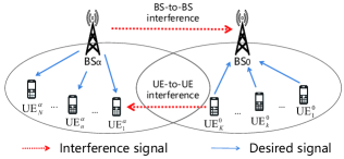
Figure 1: Illustration of CLI in a multi-cell D-TDD MIMO system.

BSs operating in the UL and DL states are $\mathbb{B}_{\text{U}}$ and $\mathbb{B}_{\text{D}}$, respectively. There are two types of CLI. On the UL, the BS₀ receives interference from the neighboring BS${}_{\alpha}\in\mathbb{B}_{\text{D}}$ that is performing DL transmission, and this type of interference is called DL-to-UL interference or BS-to-BS interference. On the DL, in addition to receiving the signal from BS_α, UE${}^{\alpha}_{1}$ also receives the UL signal of UE${}^{0}_{K}$ as interference, which is called UL-to-DL interference or UE-to-UE interference. Due to the low transmission power of UE and the high path-loss between UEs, the UL-to-DL interference is usually much weaker than the DL-to-UL interference. Therefore, in this paper, we focus on the DL-to-UL interference cancellation at the BS side. Suppose the numbers of antenna elements of UE${}^{0}_{k}$ and BS₀ are $M_{0,k}$ and $N_{0}$, respectively. The signal ${r}_{0,k}^{n_{0}}[n]$ received on the $n_{0}$th antenna element of BS₀ from UE${}^{0}_{k}$ at the $n$th sampling instant is expressed as

$${r}_{0,k}^{n_{0}}[n]=s^{n_{0}}_{0,k}[n]\!+\!{s}_{\text{D}}^{n_{0}}[n]\!+\!{s}_{\text{U}}^{n_{0}}[n]\!+\!{n}_{0,k}^{n_{0}}[n],$$ (1)

where $s^{n_{0}}_{0,k}[n]$ is the UL received signal associated with UE${}^{0}_{k}$ that is served by BS₀, ${s}_{\text{D}}^{n_{0}}[n]$ is the overall DL-to-UL interference caused by the BSs in $\mathbb{B}_{\text{D}}$ (e.g. BS_α), and ${s}^{n_{0}}_{\text{U}}[n]$ is the overall inter-user interference caused by UEs (e.g. UE${}^{\beta}_{i}$) that are served by the BSs in $\mathbb{B}_{\text{U}^{\prime}}$ (e.g. BS_β). Here we have $\mathbb{B}_{\text{U}^{\prime}}=\mathbb{B}_{\text{U}}\cup${BS₀}. In addition, ${n}^{n_{0}}_{0,k}[n]$ is the additive white Gaussian noise (AWGN). We model the link between any pair of transmit-receive antennas as a linear finite impulse response (FIR) dispersive channel, and $s^{n_{0}}_{0,k}[n]$ is expressed as

$$s^{n_{0}}_{0,k}[n]=\sum_{m_{0,k}=1}^{M_{0,k}}\sum_{l=0}^{L-1}h^{n_{0}}_{m_{0,k}}[l]u_{m_{0,k}}[n\!-\!l],$$ (2)

where $u_{m_{0,k}}[n]$ is the signal transmitted by the $m_{0,k}$th transmit antenna of UE${}^{0}_{k}$, $h^{n_{0}}_{m_{0,k}}[l]$ is the channel impulse response of the $l$th path from the $m_{0,k}$th transmit antenna of UE${}^{0}_{k}$ to the $n_{0}$th receive antenna of BS₀, and $L$ is the maximum number of multi-path components of all links[9]. For a given link, $h^{n_{0}}_{m_{0,k}}[l]$ is set to $0$ when $l$ exceeds its actual number of paths. We assume $h^{n_{0}}_{m_{0,k}}[l]\!\!=\!\!r^{-\frac{\gamma}{2}}_{0,k,l}\dot{h}^{n_{0}}_{m_{0,k}}[l]$, where $r^{-\frac{\gamma}{2}}_{0,k,l}$ characterizes the path-loss of the $l$th path from the $m_{0,k}$th antenna of UE${}^{0}_{k}$ to the $n_{0}$th antenna of BS₀, with $r_{0,k,l}$ denoting the distance between them and $\gamma$ representing the path-loss exponent, and $\dot{h}^{n_{0}}_{m_{0,k}}[l]\!\!\sim\!\!\mathcal{CN}(0,1)$ denotes the small-scale fading of the channel. Note that the impulse response of the other channels considered in this paper obeys the same model defined here. Similarly, we have

$${s}_{\text{D}}^{n_{0}}[n]\!=\!\!\sum_{\text{BS}_{\alpha}}s_{\text{D},\alpha}^{n_{0}}[n]=\!\!\sum_{\text{BS}_{\alpha}}\sum_{n_{\alpha}=1}^{N_{\alpha}}\sum_{l=0}^{L-1}h^{n_{0}}_{n_{\alpha}}[l]d_{n_{\alpha}}[n-l],$$ (3)

where ${s}_{\text{D},\alpha}^{n_{0}}[n]$ represents the DL interference imposed by BS_α on BS₀, $h^{n_{0}}_{n_{\alpha}}[l]$ is the channel impulse response of the $l$th path from the $n_{\alpha}$th transmit antenna of BS_α to the $n_{0}$th receive antenna of BS₀, and $d_{n_{\alpha}}[n]$ denotes the signal sent by the $n_{\alpha}$th antenna of BS_α. Here $N_{\alpha}$ is the number of antenna elements of BS_α. The UL interference received at BS₀ is given by

$${s}_{\text{U}}^{n_{0}}[n]\!\!=\!\!\sum_{\text{BS}_{\beta}}\sum_{\text{UE}^{\beta}_{i}}\mathbf{s}_{\text{U},\beta,i}^{n_{0}}[n]\!\!=\!\!\sum_{\text{BS}_{\beta}}\sum_{\text{UE}^{\beta}_{i}}\sum_{m_{\beta,i}}^{M_{\beta,i}}\sum_{l=0}^{L-1}h^{n_{0}}_{m_{\beta,i}}[l]u_{m_{\beta,i}}[n-l],$$ (4)

where $h^{n_{0}}_{m_{\beta,i}}[l]$ is the channel impulse response of the $l$th path from the $m_{\beta,i}$th transmit antenna of UE${}^{\beta}_{i}$ to the $n_{0}$th receive antenna of BS₀, and $u_{m_{\beta,i}}[n]$ denotes the signal sent by the $m_{\beta,i}$th antenna of UE${}^{\beta}_{i}$ that uses the same frequency band as UE${}^{0}_{k}$. Obviously, when we have $\beta=0$, ${s}^{n_{0}}_{\text{U},\beta,i}[n]$ represents intra-cell inter-user interference, and when we have $\beta\neq 0$, ${s}^{n_{0}}_{\text{U},\beta,i}[n]$ represents inter-cell inter-user interference.

The inter-cell/intra-cell inter-user interference received on the UL at BS₀ can be avoided by the inter-cell interference coordination technique of LTE/NR and eliminated by multiuser joint detection, respectively. Even if the inter-cell uplink interference could not be avoided in particular circumstances, it can still be mitigated by the multiuser joint detection based coordinated multi-point (CoMP) UL receiver [10]. Hence, ${s}_{\text{U}}^{n_{0}}[n]$ is ignored in the proposed IC scheme focusing on mitigating the BS-to-BS interference, and (1) is simplified as

$${r}_{0,k}^{n_{0}}[n]\!=\!s^{n_{0}}_{0,k}[n]\!+\!{s}_{\text{D}}^{n_{0}}[n]\!+\!{n}_{0,k}^{n_{0}}[n].$$ (5)

II-B CLI Cancellation Problem Formulation

Suppose that there is a high-capacity backhaul connection (i.e. X2-like interface) between BS₀ and BS_α to enable the exchange of inter-cell information associated with the DL transmission of BS_α [7, 8]. Then, the DL packet, the modulation and coding, the demodulation reference signals, and so forth, can be known at the BS₀. Referring to (5), typically the CSI-based traditional cancellation (TC) schemes of CLI first obtain the estimate of the channel impulse response $h^{n_{0}}_{n_{\alpha}}[l]$ [5, 8], without considering the RF chain characteristics, then reconstruct the BS-to-BS interference $\hat{s}^{n_{0}}_{\text{D},\alpha}$, $\forall\ \textrm{BS}_{\alpha}\in\mathbb{B}_{\text{D}}$, and finally subtract $\hat{s}^{n_{0}}_{\text{D}}$ from the received signal ${r}^{n_{0}}_{0,k}$ to obtain the interference-free signal ${\hat{f}}^{n_{0}}_{0,k}$, which is composed of the UL received signal associated with UE${}^{0}_{k}$ and the noise, namely

$${\hat{f}}_{0,k}^{n_{0}}={s}_{0,k}^{n_{0}}+{\bar{n}}_{0,k}^{n_{0}}={r}_{0,k}^{n_{0}}-\hat{s}^{n_{0}}_{\text{D}}={r}_{0,k}^{n_{0}}-\sum_{\text{BS}_{\alpha}}\hat{s}_{\text{D},\alpha}^{n_{0}},$$ (6)

where ${\bar{n}}_{0,k}^{n_{0}}$ consists of ${n}_{0,k}^{n_{0}}$ and the residual CLI. We note that $\hat{x}$ represents the estimate of $x$ throughout the paper. For more accurately modelling the DL-to-UL interference, a more realistic BS-to-BS channel model incorporating the RF chain characteristics is described below.

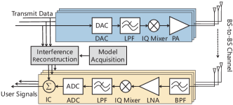
Figure 2: Block diagram of the signal reception and transmission over the BS-to-BS channel. The model acquisition module represents the acquisition of the BS-to-BS channel parameters or the training of the neural networks.

II-C BS-to-BS Interference Modelling with RF Chain Characteristics

Different from the existing contributions on CLI mitigation [5, 7, 8], where the BS-to-BS CSI matrix only comprises the path-loss and fast fading, in this paper we establish a more realistic BS-to-BS MIMO channel model that considers the major characteristics of the RF chain to perform the BS-to-BS interference modelling, as shown in Fig. 2. This approach accounts for the effects of both the channel linearity and the nonlinearity associated with the RF chain. For simplifying the analysis, we consider the impacts of the in-phase and quadrature (IQ) mixer and the power amplifier (PA), while assuming ideal digital-to-analog converter (DAC), low pass filter (LPF), band pass filter (BPF), low noise amplifier (LNA) and analog-to-digital converter (ADC).

With respect to $d_{n_{\alpha}}[n]$ in Eq. (3) and the MIMO transceiver illustrated in Fig. 2, the digital baseband signal passed through the DAC, LPF and IQ mixer is modelled as

$$d_{n_{\alpha}}^{\mathrm{IQ}}[n]=K_{1,n_{\alpha}}d_{n_{\alpha}}[n]+K_{2,n_{\alpha}}d_{n_{\alpha}}^{*}[n],$$ (7)

where we have $\left|K_{1,n_{\alpha}}\right|>>\left|K_{2,n_{\alpha}}\right|$, $K_{1,n_{\alpha}}\!=\!1/2(1+g_{n_{\alpha}}e^{j\varphi_{n_{\alpha}}})$, and $K_{2,n_{\alpha}}\!=\!1/2\left(1-g_{n_{\alpha}}e^{j\varphi_{n_{\alpha}}}\right)$, whilst $g_{n_{\alpha}}$ and $\varphi_{n_{\alpha}}$ are the gain and phase imbalance parameters of the $n_{\alpha}$th transmit antenna element, respectively. The symbol “*” denotes complex conjugate. The output signal of the IQ mixer is amplified by the PA, and the response of the PA is approximated by using the parallel Hammerstein (PH) model [11] and given as

$$d_{n_{\alpha}}^{\mathrm{PA}}[n]\!\!=\!\!\!\sum_{p=1\atop p\text{ odd }}^{P}\!\!\sum_{m=0}^{M}\!v_{n_{\alpha},p}^{\mathrm{PA}}[m]d_{n_{\alpha}}^{\mathrm{IQ}}[n\!\!-\!\!m]\left|d_{n_{\alpha}}^{\mathrm{IQ}}[n\!\!-\!\!m]\right|^{p\!-\!1}\!,$$ (8)

where $M$ is the memory length of the PA, $P$ is the order of nonlinearity considered in the PH model, and $v_{n_{\alpha},p}^{\mathrm{PA}}$ is the impulse response of the $p$th-order nonlinearity. The baseband signal received by the $n_{0}$th receive antenna of BS₀ at the $n$th sampling instant from the $n_{\alpha}$th antenna of BS_α is given by

$$s^{n_{0}}_{\text{D},\alpha}[n]=\sum_{n_{\alpha}=1}^{N_{\alpha}}\sum_{l=0}^{L-1}h^{n_{0}}_{n_{\alpha}}[l]d_{n_{\alpha}}^{\mathrm{PA}}[n-l].$$ (9)

By substituting (7) and (8) into (9), we have

$$\begin{split}s_{\text{D},\alpha}^{n_{0}}[n]=\sum_{n_{\alpha}=1}^{N_{\alpha}}\sum_{p=1\atop p\text{ odd }}^{P}&\sum_{q=0}^{p}\sum_{m=0}^{M+L-1}\omega^{n_{0}}_{n_{\alpha},p,q}[m]\\ &\times\Phi(d_{n_{\alpha}}[n-m],p,q),\end{split}$$ (10)

where $\omega^{n_{0}}_{n_{\alpha},p,q}[m]$ characterizes the overall effect of the corresponding coefficients in (7), (8) and (9), and $\Phi(x,p,q)$ equals $x^{q}(x^{*})^{p-q}$. Therefore, at the $n$th sampling instant, the CLI $\mathbf{s}_{\text{D},\alpha}$ from BS_α to BS₀ can be expressed as

$$\mathbf{s}_{\text{D},\alpha}[n]=\left[s^{1}_{\text{D},\alpha}[n],\cdots,s^{n_{0}}_{\text{D},\alpha}[n],\cdots,s^{N_{0}}_{\text{D},\alpha}[n]\right].$$ (11)

III Digital CLI Canceller

In this section, we propose three types of digital-domain CLI cancellers based on the channel model described by (10), namely the polynomial canceller (PC), the neural network canceller (NNC) and the hybrid canceller (HC). Note that both the NNC and the HC are based on ML. The metric we use to measure the performance of these CLI cancellers is $C_{\mathrm{dB}}$ (expressed in dB), which is defined over the time-window with length $N$ as

$$C_{\mathrm{dB}}\!\!=\!\!10{\color[rgb]{0,0,0}\log_{10}}\left(\frac{\sum_{n_{0}=1}^{N_{0}}\sum_{n=0}^{N-1}|s^{n_{0}}_{\text{D},\alpha}[n]|^{2}}{\sum_{n_{0}=1}^{N_{0}}\sum_{n=0}^{N-1}|s^{n_{0}}_{\text{D},\alpha}[n]-\hat{s}^{n_{0}}_{\text{D},\alpha}[n]|^{2}}\right).$$ (12)

III-A PC

When the BS-to-BS MIMO channel with the RF chain characteristics is combined with the interference cancellation philosophy, a CLI canceller that deals with the estimation of the coefficients of a polynomial, as seen in (10), is conceived. We call it the PC scheme, where the reconstructed interference $\hat{s}^{n_{0}}_{\text{D},\alpha}$ is obtained by using the data $d_{n_{\alpha}}$ of BS_α and estimating the channel parameters $\hat{\omega}^{n_{0}}_{n_{\alpha},p,q}$. We note that reliable backhaul connections are assumed between BSs, and through BS coordination a “clean” period exists, during which there is only a single interfering BS and no uplink transmission for the BS₀. Hence BS₀ is able to obtain $d_{n_{\alpha}}[n]$ and $s^{n_{0}}_{\text{D},\alpha}[n]$ for estimating $\hat{\omega}^{n_{0}}_{n_{\alpha},p,q}$ with the least squares (LS) method, before the normal data transmission takes place. Note that the NNC and the HC can also obtain the training data through this method.

For a CLI canceller both the number of real-value parameters to be estimated and the computational complexity are important metrics. Floating-point multiplication is faster than floating-point addition, while integer addition is faster than integer multiplication[12]. How much faster depends on the computer architecture, as confirmed by our extensive tests. We simply define the computational complexity as the sum of the real-value addition and multiplication operations required to reconstruct the interference signals. Since the estimation of the parameters $\hat{\omega}^{n_{0}}_{n_{\alpha},p,q}$ can be done offline before the normal data transmission takes place, we ignore the computational complexity of estimating $\hat{\omega}^{n_{0}}_{n_{\alpha},p,q}$. Since the receiver of BS₀ has $N_{0}$ antenna elements, the number of real-value parameters to be estimated in the PC approach is given as

$$n_{\text{PC}}=0.5N_{0}N_{\alpha}(M+L)\left({P+1}\right)\left({P+3}\right).$$ (13)

Addition of two complex numbers requires two real-value additions, and multiplication of two complex numbers requires four real-value multiplications, as well as one addition and one subtraction. Since modern computers use the same circuits and instructions to handle addition and subtraction, the computational complexities of addition and subtraction are regarded the same. We ignore the computational complexity of complex conjugation, hence in total we need $6^{p}$ operations for calculating $\omega^{n_{0}}_{n_{\alpha},p,q}[m]\!\!\times\!\!\Phi(x,p,q)$. As seen from (10) and (11), the computational complexity of PC is then expressed as

$$c_{\text{PC}}\!\!=\!\!N_{0}N_{\alpha}(M\!\!+\!\!L)(\frac{(35P\!\!+\!\!33)6^{P\!+\!2}\!\!+\!\!12}{35^{2}}\!+\!\frac{(P\!\!+\!\!1)(P\!\!+\!\!3)}{2})\!\!-\!\!{\color[rgb]{0,0,0}2N_{0}}.$$ (14)

A larger $P$ represents a better fit to the channel nonlinearity, but the computational complexity grows quickly with $P$, which is unbearable on a BS with limited computation resources. We can utilize ML to solve this contradiction, as presented below. Note that since different interference cancellers with different parameters can be trained by the interfered BS₀ in the multi-interfering-BS scenario independently and used in parallel, $n_{\text{PC}}$ and $c_{\text{PC}}$ of PC grow linearly with the number of BS_α. This conclusion also holds for the NNC and the HC, and our scheme can remain lightweight in more-complex scenarios.

III-B NNC

Feedforward neural network (FNN) is a multi-layer neural network, and it can be trained by splitting the data into mini-batches and executing a gradient descent update after processing each mini-batch. One pass through the entire training data set is called a training epoch.

The input ${\color[rgb]{0,0,0}\mathbf{x}[n]}\in\mathbb{R}^{2N_{\alpha}(M_{\alpha}+1)}$ of NNC is given by $[\Re{(d_{1}[n])},\Im{(d_{1}[n])},\cdots,\Re{(d_{n_{\alpha}}[n\!-\!m])},\Im{(d_{n_{\alpha}}[n\!-\!m])},\cdots,\\ \Re{(d_{N_{\alpha}}[n\!-\!M_{\alpha}])},\Im{(d_{N_{\alpha}}[n\!-\!M_{\alpha}])}]$, and the corresponding ideal output $\mathbf{y}_{\text{NNC}}[n]\in\mathbb{R}^{2N_{0}}$ is expressed as $[\Re{(s^{1}_{\text{D},\alpha}[n])},\\ \Im{(s^{1}_{\text{D},\alpha}[n])},\cdots,\Re{(s^{N_{0}}_{\text{D},\alpha}[n])},\Im{(s^{N_{0}}_{\text{D},\alpha}[n])}]$. To improve the performance and training stability of the FNN, $\mathbf{x}[n]$ is normalized to $\mathbf{x}^{\prime}=\mathbf{x}[n]^{\prime}\!\!=\!\!{\mathbf{x}[n]}/{m_{1}}$ and then fed into FNN, as shown in Fig. 3. Since FNN is trained with the label data $\mathbf{y}_{\text{NNC}}[n]^{\prime}=\mathbf{y}_{\text{NNC}}[n]/{m_{2}^{\text{NNC}}}$, the output $\mathbf{\hat{y}}_{\text{NNC}}[n]^{\prime}$ of FNN corresponding to $\mathbf{x}[n]^{\prime}$ needs to be denormalized to $\mathbf{\hat{y}}_{\text{NNC}}[n]=m_{2}^{\text{NNC}}\mathbf{\hat{y}}_{\text{NNC}}[n]^{\prime}$ before interference cancellation. Note that $m_{1}$ and $m_{2}^{\text{NNC}}$ are the maximum values of $|d_{n_{\alpha}}[n]|$ and $|s^{n_{0}}_{\text{D},\alpha}[n]|$, respectively.

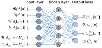
Figure 3: An FNN with $2N_{\alpha}(M_{\alpha}+1)$ input nodes, $N_{h}$ hidden nodes, and $2N_{0}$ output nodes, where we have $M_{\alpha}=M+L-1$.

The parameters of the FNN considered are all real-valued. In the three-layer FNN shown in Fig. 3, we suppose the numbers of nodes on the input layer, hidden layer and output layer are $N_{\text{in}}$, $N_{\text{h}}$ and $N_{\text{out}}$, respectively. The function from the input layer to the hidden layer can be expressed as $\mathbf{x}_{\text{h}}\!\!=\!\!\sigma(\mathbf{W}_{\text{h}}{\color[rgb]{0,0,0}\mathbf{x}^{\prime}}+\mathbf{b}_{\text{h}})$, where $\mathbf{W}_{\text{h}}\in\mathbb{R}^{N_{\text{h}}\times N_{\text{in}}}$ is the parameter matrix, $\mathbf{b}_{\text{h}}\in\mathbb{R}^{N_{\text{h}}}$ is the bias, and $\sigma(x)$ represents the nonlinear activation function, which enables the FNN to well fit the nonlinear relationship between the inputs and the outputs. Therefore, there are totally $(N_{\text{in}}+1)N_{\text{h}}$ parameters in $\mathbf{W}_{\text{h}}$ and $\mathbf{b}_{\text{h}}$. In addition, $N_{\text{in}}N_{\text{h}}$ multiplications, $N_{\text{in}}N_{\text{h}}$ additions and $c_{\sigma}N_{\text{h}}$ comparison operations in $\mathbb{R}$ are required for calculating $\sigma(\mathbf{W}_{\text{h}}{\color[rgb]{0,0,0}\mathbf{x}^{\prime}}+\mathbf{b}_{\text{h}})$, where ${\color[rgb]{0,0,0}c_{\sigma}}$ represents the complexity of calculating $\sigma(x)$. In this paper, we choose $\sigma(x)=\max(0,x)$, which is a numeric comparison operation, so we set ${\color[rgb]{0,0,0}c_{\sigma}}=1$. Similarly, without considering the activation function, the number of parameters and the computational complexity of calculation from the hidden layer to the output layer are $(N_{\text{h}}+1)N_{\text{out}}$ and $2N_{\text{h}}N_{\text{out}}$, respectively. Besides, $N_{\text{in}}$ and $N_{\text{out}}$ multiplications, as well as two parameters $1/m_{1}$ and $m_{2}^{\text{NNC}}$, are needed for normalization and denormalization, respectively.

Based on (10) and (11), we have $N_{\text{in}}=2N_{\alpha}(M+L)$ and $N_{\text{out}}=2N_{0}$. Moreover, $N_{\text{in}}$ belongs to hyperparameters that are tunable. Therefore, the number of parameters $n_{\text{NNC}}$ and the computational complexity $c_{\text{NNC}}$ of NNC are given by

$$n_{\text{NNC}}=N_{\text{h}}[2(M+L)N_{\alpha}+2N_{0}+1]+2N_{0}+2,$$ (15)

$$c_{\text{NNC}}=2(2N_{\text{h}}+1)[N_{\alpha}(M+L)+N_{0}]+{\color[rgb]{0,0,0}c_{\sigma}}N_{\text{h}},\vspace{-5pt}$$ (16)

respectively, while $n_{\text{NNC}}$ and $c_{\text{NNC}}$ are independent of the nonlinearity order $P$.

III-C HC

The CLI signal of (10) can be decomposed as

$$s_{\text{D},\alpha}^{n_{0}}[n]=s^{n_{0},\text{lin}}_{\text{D},\alpha}[n]+s^{n_{0},\text{nl}}_{\text{D},\alpha}[n],$$ (17)

where $s^{n_{0},\text{lin}}_{\text{D},\alpha}[n]$ and $s^{n_{0},\text{nl}}_{\text{D},\alpha}[n]$ represent the linear part and nonlinear part of $s_{\text{D},\alpha}^{n_{0}}[n]$, respectively. The linear part corresponds to the terms when we have $P=1$ and $q=1$ in Eq. (10), and the nonlinear part corresponds to the rest. If the linear part is eliminated and the nonlinear part is ignored, HC degenerates into TC. The HC approach can be divided into two steps. First, the TC is invoked to estimate the linear part as $\hat{s}^{n_{0},\text{lin}}_{\text{D},\alpha}[n]$. Second, the NNC is used to estimate the remaining nonlinear part as $\hat{s}^{n_{0},\text{nl}}_{\text{D},\alpha}[n]\!\!=\!\!s^{n_{0}}_{\text{D},\alpha}[n]\!-\!\hat{s}^{n_{0},\text{lin}}_{\text{D},\alpha}[n]$. In other words, FNN is trained with the input data $\mathbf{x}[n]^{\prime}\!\!=\!\!{\mathbf{x}[n]}/{m_{1}}$ and the label data $\mathbf{y}_{\text{HC}}[n]^{\prime}\!=\!\mathbf{y}_{\text{HC}}[n]/{m_{2}^{\text{HC}}}$, where $\mathbf{y}_{\text{HC}}[n]$ is expressed as $[\Re{(\hat{s}^{1,\textrm{nl}}_{\text{D},\alpha}[n])},\Im{(\hat{s}^{1,\textrm{nl}}_{\text{D},\alpha}[n])},\cdots,\Re{(\hat{s}^{N_{0},\textrm{nl}}_{\text{D},\alpha}[n])},\Im{(\hat{s}^{N_{0},\textrm{nl}}_{\text{D},\alpha}[n])}]$ and $m_{2}^{\text{HC}}$ is the maximum value of $|\hat{s}^{n_{0},\textrm{nl}}_{\text{D},\alpha}[n]|$. We note that, because of the low power of the nonlinear part, reconstructing CLI signals by only using ML may cause the nonlinear part to be ignored. Similarly, the number of parameters and the computational complexity of the HC can be expressed respectively as

$$n_{\text{HC}}=2N_{0}N_{\alpha}(M+L)+n_{\text{NNC}},$$ (18)

$$c_{\text{HC}}=8N_{0}N_{\alpha}(M+L)-{\color[rgb]{0,0,0}2N_{0}}+c_{\text{NNC}}.$$ (19)

IV Experimental Results

In this section, we present the numerical results to compare the performance of the PC, the NNC and the HC methods.

TABLE I: Relevant Parameters of BS-to-BS Transmission

Parameters	Values
Received CLI power	-52.1 dBm
Transmitting power of the interfering BS	47 dBm
AWGN power	-90 dBm
Waveform	OFDM
Bandwidth	13MHz
Sampling frequency	120MHz
ADC resolution	12
Number of TX/RX antennas	4/4
Fading distribution	Rayleigh
Memory length of the PA ($M$)	2
Maximum number of multi-path components ($L$)	7
Nonlinearity order of the interference canceller ($P$)	3
Batch size of the FNN	32
Learning rate of the FNN	$2\times 10^{-4}$
Loss function of the FNN	Mean squared error
Optimization algorithm of the FNN	Adam

IV-A Data Set

We study the performance of the PC, the NNC and the HC methods through system level simulations of a D-TDD MIMO system, and the main simulation parameters are shown in Table I. For the sake of simplicity, the number of BSs is set to 2. The interfered BS obtains 50000 baseband samples $d_{n_{\alpha}}$ from the interfering BS per transmit antenna via the backhaul connection, and obtains the corresponding CLI $s^{n_{0}}_{\text{D},\alpha}$ per receive antenna relying on its own ADC. We note that 80% data are used for training and 20% data for testing.

IV-B Numerical Results

In Fig. 4, on the one hand, it is observed that the number of parameters of the PC increases linearly with the order of nonlinearity $P$ assumed, while its computational complexity grows exponentially with $P$. Moreover, the number of parameters and the computational complexity of both the ML based cancellers increase linearly with the number of hidden nodes $N_{h}$. On the other hand, we characterize how the IC performance of different CLI cancellers changes with $P$ and $N_{h}$. For the PC, $P\!=\!3$ is used, since a larger $P$ leads to excessive computational complexity and slightly improved IC performance. For the NNC and HC, we set $N_{\text{h}}=300$ and $N_{\text{h}}=200$, respectively, to achieve high IC performance, small number of parameters to be estimated and low computational complexity. Therefore, the numbers of parameters of the CLI cancellers are $n_{\text{PC}}\!=\!1728$, $n_{\text{NNC}}\!=\!24310$ and $n_{\text{HC}}\!=\!16498$, respectively, while their computational complexities are $c_{\text{PC}}\!=\!{\color[rgb]{0,0,0}127864}$, $c_{\text{NNC}}\!=\!48380$ and $c_{\text{HC}}\!=\!{\color[rgb]{0,0,0}33424}$, respectively.

In Fig. 5 we compare the IC performance in terms of the residual CLI power upon using different CLI cancellers. The noise floor power is $-90$dBm, which is the lower limit of the residual CLI power. The power of CLI received by the interfered BS₀ is $-52.1$dBm, which is the upper limit of the residual CLI power. A residual CLI of $-73.3$dBm remains upon using the TC, thus the CLI cancellation performance of $C_{\mathrm{dB}}\!\!=\!\!21.2\text{dB}$ is achieved by the TC. In contrast, the CLI cancellation performances of the PC, the NNC and the HC are $C_{\mathrm{dB}}\!\!=\!\!32.7\text{dB}$, $C_{\mathrm{dB}}\!\!=\!\!30.4\text{dB}$ and $C_{\mathrm{dB}}\!\!=\!\!35.9\text{dB}$, respectively.

In Fig. 6, we observe that the NNC and the HC converge and reach the peak of the IC performance after training a small number of epochs, which facilitates the deployment of the NNC and HC methods in realistic networks.

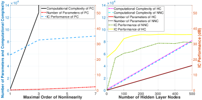
Figure 4: The number of parameters, the computational complexity, the IC performance of the PC as a function of the order of nonlinearity (left), and those of the NNC and HC as a function of the number of hidden nodes (right).

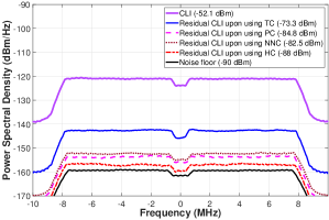
Figure 5: Comparison of the IC performance in terms of the residual CLI power upon using different CLI cancellers, against the power of the received CLI and of the noise floor, which is the variance of ${n}^{n_{0}}_{0,k}$ in (1).

V Conclusion

We first propose a more realistic BS-to-BS channel model accounting for the effects of both the channel linearity and nonlinearity associated with the RF chain. Based on this model we propose three digital-domain CLI cancellers, namely the PC, NNC and HC. We demonstrate through analysis and numerical simulations that the three cancellers are able to achieve at least 43.4% CLI cancellation performance improvement compared with the traditional CSI-based interference canceller. Among them, the PC has the least number of parameters. Compared with that of the PC, the computational complexities of both lightweight-ML based cancellers are reduced by more than 62.2%, and the HC, which deals with the linear and nonlinear CLI components differentially, has the highest CLI cancellation performance ($C_{\mathrm{dB}}=35.9\text{dB}$) and the lowest computational complexity.

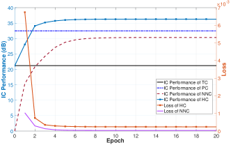
Figure 6: The achievable IC performance ($C_{\mathrm{dB}}$) (left axis), and the loss of the NNC and the HC (right axis), as a function of the number of epochs. The $\mathsf{loss}$ functions of NNC and HC are expressed as $\frac{1}{N}\sum_{n=1}^{N}\left\|{\mathbf{y}_{\text{NNC}}[n]}/{m_{2}^{\text{NNC}}}-\mathbf{\hat{y}}_{\text{NNC}}[n]^{\prime}\right\|_{2}^{2}$ and $\frac{1}{N}\sum_{n=1}^{N}\left\|{\mathbf{y}_{\text{HC}}[n]}/{m_{2}^{\text{HC}}}-\mathbf{\hat{y}}_{\text{HC}}[n]^{\prime}\right\|_{2}^{2}$, respectively.

References

- [1] Z. Shen, A. Khoryaev, E. Eriksson, and X. Pan, “Dynamic uplink-downlink configuration and interference management in TD-LTE,” IEEE Communications Magazine, vol. 50, no. 11, pp. 51–59, Nov. 2012.
- [2] Z. Huo, N. Ma, and B. Liu, “Joint user scheduling and transceiver design for cross-link interference suppression in MU-MIMO dynamic TDD systems,” in Proc. 3rd IEEE/CIC International Conference on Computer and Communications (ICCC), Chengdu, China, Dec. 2017, pp. 962–967.
- [3] Q. Chen, H. Zhao, L. Li, H. Long, J. Wang, and X. Hou, “A closed-loop UL power control scheme for interference mitigation in dynamic TD-LTE systems,” in Proc. 81st IEEE Vehicular Technology Conference (VTC Spring), Glasgow, UK, Jul. 2015, pp. 1–5.
- [4] E. de Olivindo Cavalcante, G. Fodor, Y. C. B. Silva, and W. C. Freitas, “Distributed beamforming in dynamic TDD MIMO networks with BS to BS interference constraints,” IEEE Wireless Communications Letters, vol. 7, no. 5, pp. 788–791, Oct. 2018.
- [5] K. Lee, Y. Park, M. Na, H. Wang, and D. Hong, “Aligned reverse frame structure for interference mitigation in dynamic TDD systems,” IEEE Transactions on Wireless Communications, vol. 16, no. 10, pp. 6967–6978, Oct. 2017.
- [6] S. Lagen, A. Agustin, and J. Vidal, “Joint user scheduling, precoder design, and transmit direction selection in MIMO TDD small cell networks,” IEEE Transactions on Wireless Communications, vol. 16, no. 4, pp. 2434–2449, Apr. 2017.
- [7] M. Ding, D. L. Pcoqrez, A. V. Vasilakos, and W. Chen, “Dynamic TDD transmissions in homogeneous small cell networks,” in Proc. IEEE International Conference on Communications (ICC) Workshops, Sydney, Australia, Jun. 2014, pp. 616–621.
- [8] Dynamic TDD Interference Mitigation Concepts in NR, document R1-1703110, TSG RAN WG1 Meeting #88, 3GPP, Sophia Antipolis, France, Feb. 2017.
- [9] S. Yang and L. Hanzo, “Fifty years of MIMO detection: The road to large-scale MIMOs,” IEEE Communications Surveys & Tutorials, vol. 17, no. 4, pp. 1941–1988, Fourth Quarter 2015.
- [10] S. Yang, T. Lv, R. G. Maunder, and L. Hanzo, “Distributed probabilistic-data-association-based soft reception employing base station cooperation in mimo-aided multiuser multicell systems,” IEEE Transactions on Vehicular Technology, vol. 60, no. 7, pp. 3532–3538, Sep. 2011.
- [11] M. Isaksson, D. Wisell, and D. Ronnow, “A comparative analysis of behavioral models for RF power amplifiers,” IEEE Transactions on Microwave Theory and Techniques, vol. 54, no. 1, pp. 348–359, Jan. 2006.
- [12] IEEE Standard for Floating-Point Arithmetic, Std. IEEE Std 754-2019 (Revision of IEEE 754-2008), Jul. 2019.