Rationally Extended Harmonic Oscillator potential, Isospectral Family and the Uncertainity Relations

Abstract

We consider the rationally extended harmonic oscillator potential which is isospectral to the conventional one and whose solutions are associated with the exceptional, $X_{m}$- Hermite polynomials and discuss its various important properties for different even codimension of $m$. The uncertainty relations are obtained for different $m$ and it is shown that for the ground state, the uncertainity increases as $m$ increases. A one parameter $(\lambda)$ family of exactly solvable isospectral potential corresponding to this extended harmonic oscillator potential is obtained. Special cases corresponding to the $\lambda=0$ and $\lambda=-1$, which give the Pursey and the Abhram-Moses potentials respectively, are discussed. The uncertainty relations for the entire isospectral family of potentials for different $m$ and $\lambda$ are also calculated.

$~{}^{a}$Department of Physics, Model College, Dumka-814101, India.
$~{}^{b}$Department of Physics, S. K. M. University, Dumka-814110, India.
$~{}^{c}$Department of Physics, Savitribai Phule Pune University, Pune-411007, India.

1 Introduction

The idea of Supersymmetric Quantum Mechanics(SQM) [1] is not only useful in solving the quantum mechanical potential problems but has also opened the scope for discovering new exactly solvable potentials. These potentials have applications in diverse areas like inverse scattering [2, 3], soliton theory [4, 5], etc. This sparked a race among researchers to search for a family of isospectral potentials [6, 7, 8, 9]. To accomplish this purpose, several methods were developed like Darboux transformation [10], Darboux Crum Krein Adler Transformation [11], SQM [12, 13], etc. Popular among them was the SQM approach due to its simplicity and it was shown using this approach that for any 1-D potential with atleast one bound state, one can always construct one continuous parameter family of strictly isospectral potentials.

The discovery of the $X_{m}$-exceptional orthogonal polynomials (EOPs) [14, 15, 16] paved the path for discovering new rationally extended shape invariant potentials whose eigenfunctions are in terms of these EOPs. Various properties of these potentials have been studied in detail in [17, 18, 19, 20, 21, 22, 23, 24, 25, 26, 27, 28, 29] and the references therein. After the discovery of the exceptional Hermite polynomials [30], Fellows and Smith [31] discovered rationally extended one dimensional harmonic oscillator potentials. Their work has been further extended using the SQM approach [32].

The one dimensional harmonic oscillator potential is one of the most important potential having numerous applications. However, so far as we are aware off, there has not been much progress in studying the various properties of the rationally extended family of harmonic oscillator (REHO) potentials. The purpose of this paper is to take a step in that direction. Firstly, we calculate the Heisenberg uncertainty relation $\Delta x\Delta p$ for the REHO potentials. Further, we follow the idea of SQM [1], and generate a one parameter $(\lambda)$ family of rationally extended strictly isospectral potentials including the corresponding Pursey and the Abrahm-Mosses potentials and obtain their eigenfunctions explicitly in terms of the $X_{m}$-Hermite EOPs. We calculate the Heisenberg uncertainty relations for the one parameter family of rationally extended isospectral potentials (including the corresponding Pursey and the Abrahm-Mosses potentials) for different $m$ and $\lambda$.

The plan of the paper is as follows: In Sec. $2$, we briefly discuss the formulation of SQM. In Sec. $3$, we summarise the known important results related to the rationally extended harmonic oscillator potentials. A one parameter $\lambda$ family of isospectral potentials (including the corresponding Pursey and Abrahm-Mosses potentials) are obtained in Sec. $4$ for any even integral $m$. In Sec. $5$, we follow the results discussed in Sec. $3$ and Sec. $4$ and calculate the Heisenberg uncertainty relations for REHO and their isospectral family of potentials (including the corresponding Pursey and Abrahm-Mosses potentials). Finally, we summarize our results and mention some open possible problems in Sec. $6$.

2 SQM Formalism

In SQM approach, one considers the Hamiltonian (in the units $\hbar=2m=1$)

$$H^{-}=-\frac{d^{2}}{dx^{2}}+V^{-}(x)-\epsilon\;$$ (1)

where $\epsilon$ is the factorization energy. By assuming the ground state energy of this Hamiltonian $E^{-}_{0}=0$, we factorize $H^{-}$ in terms of $A$ and $A^{\dagger}$ as

$$H^{-}=A^{\dagger}A\;$$ (2)

with

$$A=\frac{d}{dx}+W(x),\qquad A^{\dagger}=-\frac{d}{dx}+W(x).$$ (3)

Here $W(x)$ is known as superpotential which is expressed in term of the ground state eigenfunction as $W(x)=-\ln[\psi^{-}_{0}(x)]^{\prime}$. In this way, another set of Hamiltonian can easily be constructed by reversing the order of the operators $A$ and $A^{\dagger}$ i.e.,

$$H^{+}=AA^{\dagger}=-\frac{d^{2}}{dx^{2}}+V^{+}(x)-\epsilon\;.$$ (4)

Thus, the partner potentials $V^{\mp}(x)$ in term of superpotential are given by

$$V^{\mp}(x)=W(x)^{2}\mp W(x)^{\prime}+\epsilon\;.$$ (5)

Here a prime denotes a derivative with respect to $x$. The precise relationship between the energies and the eigenfunctions of the partner Hamiltonians are

$$E^{-}_{n+1}=E^{+}_{n}\;>0,\qquad n=0,1,2,\cdots,$$ (6)

$$\psi^{-}_{n+1}(x)=\sqrt{\frac{1}{E^{+}_{n}}}A^{\dagger}\psi^{+}_{n}(x),\qquad\psi^{+}_{n}(x)=\sqrt{\frac{1}{E^{-}_{n+1}}}A\psi^{-}_{n+1}(x).$$ (7)

The ground state eigenfunction $\psi^{-}_{0}(x)$ is obtained by solving the differential equation,

$$A\psi^{-}_{0}(x)=0.$$ (8)

One parameter family of isospectral potentials are obtained by redefining the form of the superpotential

$$\hat{W}=W(x)+\phi(x),$$ (9)

and by assuming the uniqueness of the partner potential $V^{+}(x)$ i.e.,

$$V^{+}(x)=\hat{W}(x)^{2}+\hat{W}(x)^{\prime}+\epsilon=W(x)^{2}+W(x)^{\prime}+\epsilon,$$

which gives

$$\phi^{2}(x)+2W\phi+\phi^{\prime}(x)=0.$$

We then find that on substituting $\phi(x)=y^{-1}(x)$, the above equation satisfies the Bernoulli equation

$$y^{\prime}(x)=1+2W(x)y(x),$$

whose solution is

$$\phi(x)=\frac{d}{dx}\ln\left[\mathcal{I}(x)+\lambda\right].$$

Here $\mathcal{I}(x)=\int^{x}_{\infty}\psi^{-}_{0}(x^{\prime})^{2}\;dx^{\prime}$ and $\lambda$ is an integration constant.

Therefore, the potential which is strictly isospectral to $V^{-}(x)$ is given by

$$\hat{V}^{-}(\lambda,x) =\hat{W}(x)^{2}-\hat{W}(x)^{\prime}+\epsilon$$

$$=V^{-}(x)-2\frac{d^{2}}{dx^{2}}\ln\left[\mathcal{I}(x)+\lambda\right]\,,$$ (10)

where either $\lambda>0$ or $\lambda<-1$ so as to avoid singularity (For details, see[1, 33]). The normalized ground state eigenfunction for the entire family of potentials is given by

$$\hat{\psi}^{-}_{0}(\lambda,x)=\sqrt{\lambda(1+\lambda)}\;\frac{\psi^{-}_{0}(x)}{\mathcal{I}(x)+\lambda}\,.$$ (11)

The normalized excited states eigenfunctions can be easily calculated similar to (7) as

$$\hat{\psi}^{-}_{n+1}(\lambda,\;x) =\sqrt{\frac{1}{E^{+}_{n}}}\hat{A}^{\dagger}\psi^{+}_{n}(x)=\frac{1}{E^{-}_{n+1}}\hat{A}^{\dagger}A\psi^{-}_{n+1}(x),\qquad n=0,1,2,\cdots,$$ (12)

$$\hat{A}^{\dagger} =-\frac{d}{dx}-\frac{d}{dx}\ln\left[\frac{\psi^{-}_{0}(x)}{\mathcal{I}(x)+\lambda}\right],\qquad A=\frac{d}{dx}-\frac{d}{dx}\ln\left[\psi^{-}_{0}(x)\right]$$

and the Hamiltonian is defined similar to (1) as

$$\hat{H}^{-} =\hat{A}^{\dagger}\hat{A}=-\frac{d^{2}}{dx^{2}}+\hat{V}^{-}(x)-\epsilon$$ (13)

$$\hat{A} =\frac{d}{dx}-\frac{d}{dx}\ln\left[\frac{\psi^{-}_{0}(x)}{\mathcal{I}(x)+\lambda}\right]$$

It is worth reminding that all these strictly isospectral family of potentials have same partner potential $V^{+}(x)$.

In the limit $\lambda=0$ there is a loss of a bound state and the corresponding potential is called the Pursey potential $\hat{V}^{P}(x)$. An analogous situation occurs in the limit $\lambda=-1$ and the potential is called the Abraham-Moses potential $\hat{V}^{AM}(x)$. The normalized eigenfunctions of $\hat{V}^{P}(x)$ are given by

$$\hat{\psi}^{P}_{n}(x)=\frac{1}{E^{-}_{n+1}}\left(-\frac{d}{dx}-\frac{d}{dx}\ln\left[\frac{\psi^{-}_{0}(x)}{\mathcal{I}(x)}\right]\right)A\psi^{-}_{n+1}(x),\qquad n=0,1,2,\cdots,.$$ (14)

Similarly, the normalized eigenfunctions of $\hat{V}^{AM}(x)$ are given by

$$\hat{\psi}^{AM}_{n}(x)=\frac{1}{E^{-}_{n+1}}\left(-\frac{d}{dx}-\frac{d}{dx}\ln\left[\frac{\psi^{-}_{0}(x)}{\mathcal{I}(x)-1}\right]\right)A\psi^{-}_{n+1}(x),\qquad n=0,1,2,\cdots,.$$ (15)

The energy eigenvalues of the Pursey and the Abraham-Moses Hamiltonians obtained by substituting $\lambda$ equal to $0$ and $-1$ respectively in (13) has the same expressions as that of $H^{+}(x)$, i.e.

$$\hat{E}^{P}_{n}=\hat{E}^{AM}_{n}=E^{+}_{n},\qquad n=0,1,2,3,\cdots$$ (16)

3 REHO Potential

In this section, we briefly review the results obtained in [31, 32] about the REHO potentials. These authors extended the conventional one-dimensional harmonic oscillator potential ($V(x)=x^{2}$) using the idea of SQM and obtained the REHO potentials valid for even co-dimension of $m=0,2,4,....$ and are given by

$$V^{-}_{m}(x)=V(x)-2\left[\frac{\mathcal{H}_{m}^{\prime\prime}}{\mathcal{H}_{m}}-\left(\frac{\mathcal{H}_{m}^{\prime}}{\mathcal{H}_{m}}\right)^{2}+1\right],$$ (17)

where $\mathcal{H}_{m}(x)=(-1)^{m}H_{m}(ix)$ is pseudo-hermite polynomials and factorization energy used in the calculation was $\epsilon=-2m-1$. The normalized ground state eigenfunction $\psi^{-}_{0,m}(x)$ having zero eigenvalue and the excited states eigenfunction$\psi^{-}_{n+1,m}(x)$ for different $m$ are

$$\psi^{-}_{0,m}(x)=\left(\frac{2^{m}m!}{\sqrt{\pi}}\right)^{\frac{1}{2}}\frac{e^{-\frac{x^{2}}{2}}}{\mathcal{H}_{m}(x)},$$ (18)

and

$$\psi^{-}_{n+1,m}(x)=\frac{1}{\sqrt{E^{+}_{n,m}\;2^{n}n!\sqrt{\pi}}}\;\frac{e^{-\frac{x^{2}}{2}}}{\mathcal{H}_{m}(x)}y^{m}_{n+1}(x)\;,\qquad n=0,1,2...,$$ (19)

respectively. Here $y^{m}_{n+1}(x)=\left[\mathcal{H}_{m}(x)H_{n+1}(x)+\mathcal{H}_{m}(x)^{\prime}H_{n}(x)\right]$ and $n=-1,\;0,\;1,\;2,\dots$ is the Exceptional Hermite Polynomial. Note that $y^{m}_{0}(x)=1$. The whole system $\{y^{m}_{n+1}(x)\}$ is the exceptional orthogonal polynomial system, $X_{m}$, of co-dimension $m$ and is orthogonal and complete with respect to the positive-definite measure $\frac{e^{-x^{2}}}{\mathcal{H}_{m}(x)^{2}}$. The Hamiltonian $H^{-}_{m}$ defined similar to (1) has the energy eigenvalues $E^{-}_{n,m}$ given by

$$E^{-}_{n+1,m}=2(n+m+1),\quad n=0,1,2,\cdots,\quad\text{and }E^{-}_{0,m}=0.$$ (20)

It is seen that the difference in energy eigenvalues is $2(m+1)$ units between ground state and first excited state and 2 units between any successive excited states. Therefore energy spectra is equidistant only for $m=0$. Note that $V^{-}_{m}(x)$ is singular at $x=0$ for odd $m$ and therefore $m$ is restricted to positive even integers only.

It is worth noting that the complete set of eigenfunctions for the $m=0$ case, i.e. the one dimensional harmonic oscillator, can be reduced to a single formula containing ground state eigenfunction and excited state eigenfunction given by

$$\Psi_{\nu}(x)=\frac{1}{\sqrt{2^{\nu}\nu!\sqrt{\pi}}}e^{-\frac{x^{2}}{2}}H_{\nu}(x),\qquad\nu=0,\;1,\;2,\cdots\,.$$

The plot of the ground, first and the second excited state eigenfunctions as well as the potential versus position for $m=0,\;m=2\text{ and }m=4$ are given in Fig-1.a ,Fig-1.b and Fig-1.c respectively. It is interesting to note from these figures that as $m$ increases, the eigenfunctions and the potential well becomes sharper. In Table $1$ we have given expressions for the potential $V^{-}_{m}(x)$ as well as the ground and the excited state eigenfunctions in case $m=0,2,4$. Expressions for exceptional Hermite polynomials $y^{m}_{n+1}$ are given in Table $2$ in case $n=0,1,2$ and $m=0,2,4$.

The superpotential $W(x)$ corresponding to the REHO potential is easily obtained from the ground state eigenfunctions $\psi^{-}_{0,m}(x)$ of $V^{-}_{m}(x)$ as

$$W(x) = -\ln[\psi^{-}_{0,m}(x)]^{\prime}$$ (21)

$$= x+\frac{\mathcal{H}_{m}(x)^{\prime}}{\mathcal{H}_{m}(x)}.$$

The energy eigenvalues of the partner Hamiltonians $H^{\mp}(x)$, defined using (1) and (4), are given by

$$E^{-}_{n+1,m} =2(n+m+1),\quad n=0,1,2,\cdots,\quad\text{with}\quad E^{-}_{0,m}=0.$$ (22)

$$E^{+}_{n,m} =2(n+m+1),\quad n=0,1,2,\cdots$$ (23)

m	$V^{-}_{m}(x)$	$\psi^{-}_{0,m}(x)$	$\psi^{-}_{n+1,m}(x),\quad n=0,1,2\cdots\quad$
0	$x^{2}-2$	$\frac{1}{\sqrt[4]{\pi}}e^{-\frac{x^{2}}{2}}$	$\frac{1}{\sqrt{2(n+1)2^{n}n!\sqrt{\pi}}}e^{-\frac{x^{2}}{2}}y^{0}_{n+1}(x)$
2	$x^{2}-2+\frac{8\left(2x^{2}-1\right)}{\left(2x^{2}+1\right)^{2}}$	$\frac{2\sqrt{2}}{\sqrt[4]{\pi}}\frac{e^{-\frac{x^{2}}{2}}}{4x^{2}+2}$	$\frac{1}{\sqrt{2(n+3)2^{n}n!\sqrt{\pi}}}\frac{e^{-\frac{x^{2}}{2}}}{4x^{2}+2}y^{2}_{n+1}(x)$
4	$x^{2}-2+\frac{16\left(8x^{6}+12x^{4}+18x^{2}-9\right)}{\left(4\left(x^{2}+3\right)x^{2}+3\right)^{2}}$	$\frac{8\sqrt{6}}{\sqrt[4]{\pi}}\frac{e^{-\frac{x^{2}}{2}}}{16x^{4}+48x^{2}+12}$	$\frac{1}{\sqrt{2(n+5)2^{n}n!\sqrt{\pi}}}\frac{e^{-\frac{x^{2}}{2}}}{16x^{4}+48x^{2}+12}y^{4}_{n+1}(x)$

Table 1: Rationally extended harmonic oscillator potential $V^{-}_{m}(x)$, its ground and excited state wavefunctions for $m=0,2$ and $4$.

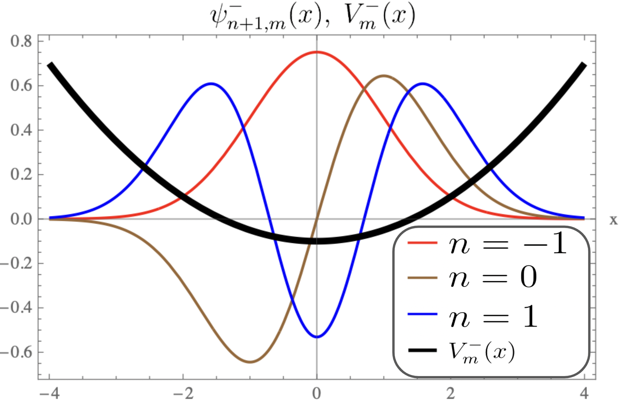
(a) m=0

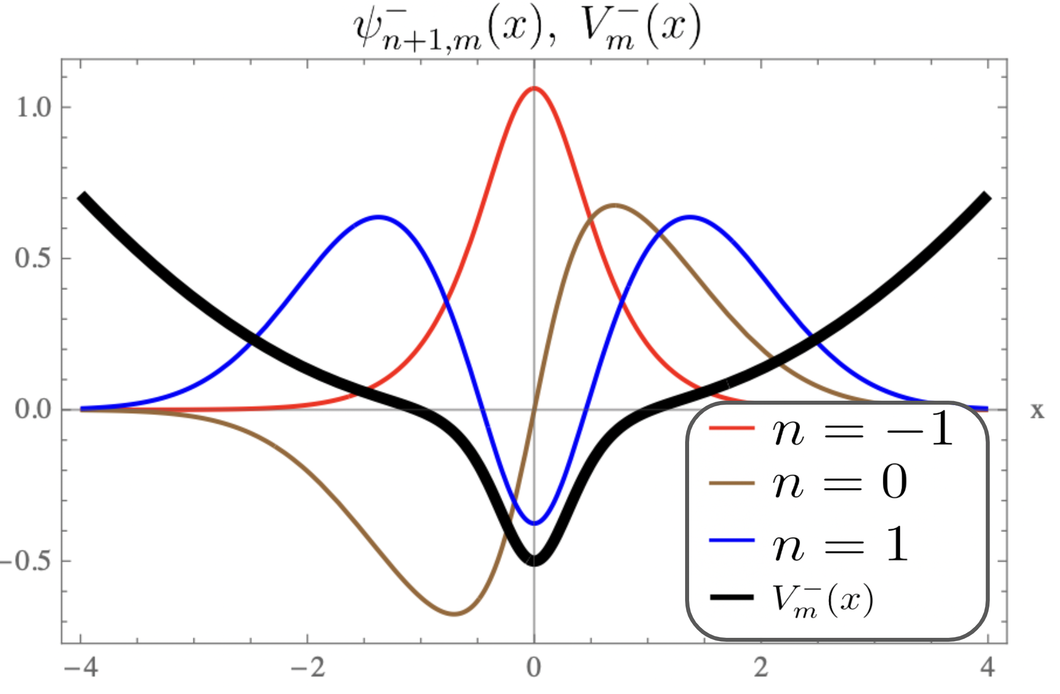
(b) m=2

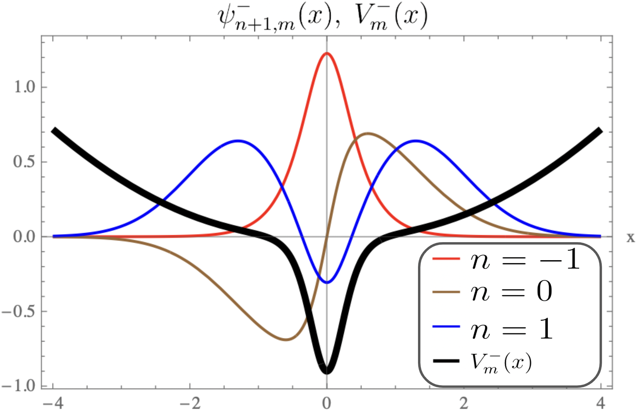
(c) m=4

Figure 1: Plots of potentials $V^{-}_{m}(x)$ and eigenfunction $\psi^{-}_{n+1,m}(x)$ as a function of $x$ for $m=0,\;2\text{ and }4$. Potentials are shown in black color.

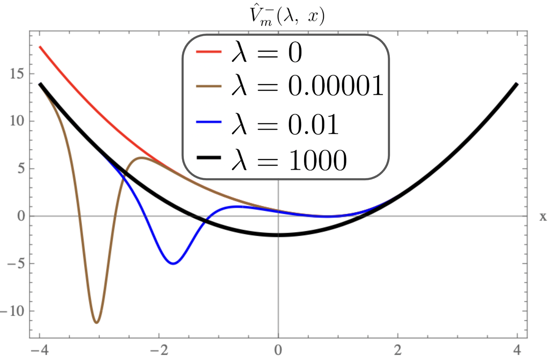
(a) Plot of $\hat{V}^{-}_{0}(\lambda,x)$ as a function of $x$ for positive $\lambda$.

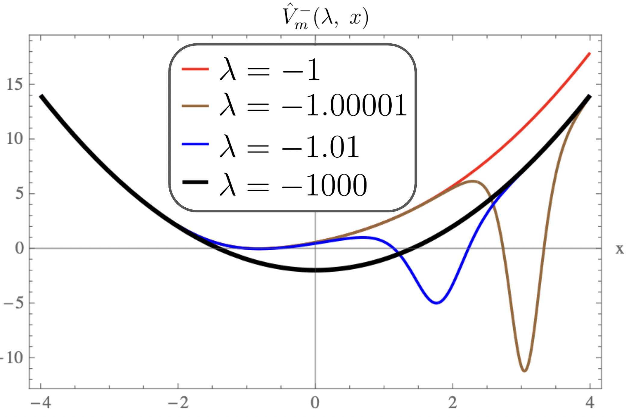
(b) Plot of $\hat{V}^{-}_{0}(\lambda,x)$ as a function of $x$ for negative $\lambda$.

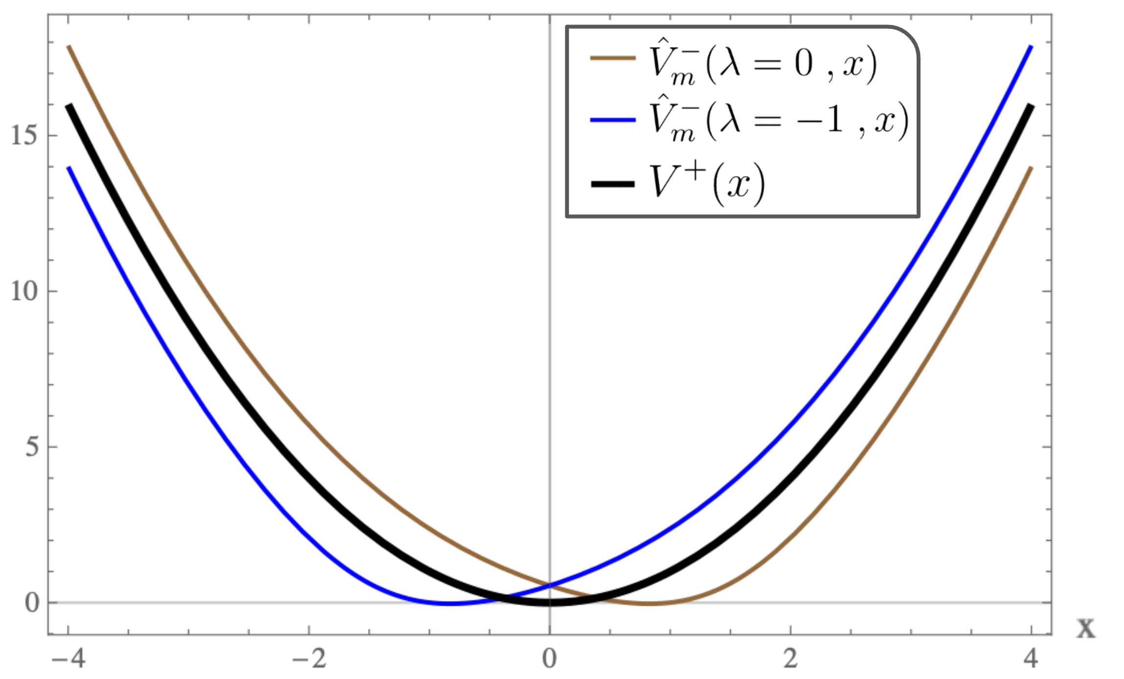
(c) Plot of Pursey $\hat{V}^{-}_{0}(0,x)$, AM $\hat{V}^{-}_{0}(-1,x)$ and $V^{+}(x)$ potential as a function of $x$

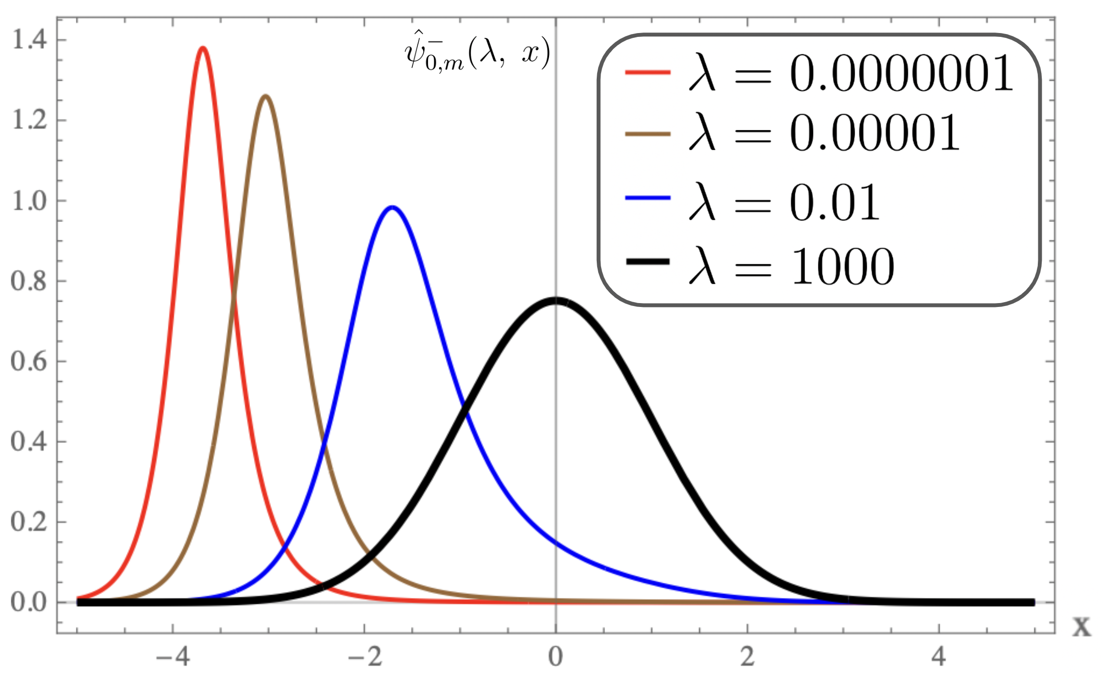
(d) Plot of Ground-state wavefunction $\hat{\psi}^{-}_{0,0}(\lambda,x)$ as a function of $x$ for various positive $\lambda$.

Figure 2: Plot of isospectral potential $\hat{V}^{-}_{0}(\lambda,x)$ and its ground state eigenfunction $\hat{\psi}^{-}_{0,0}(\lambda,x)$ as a function of $x$ for various $\lambda$ when $m=0$.

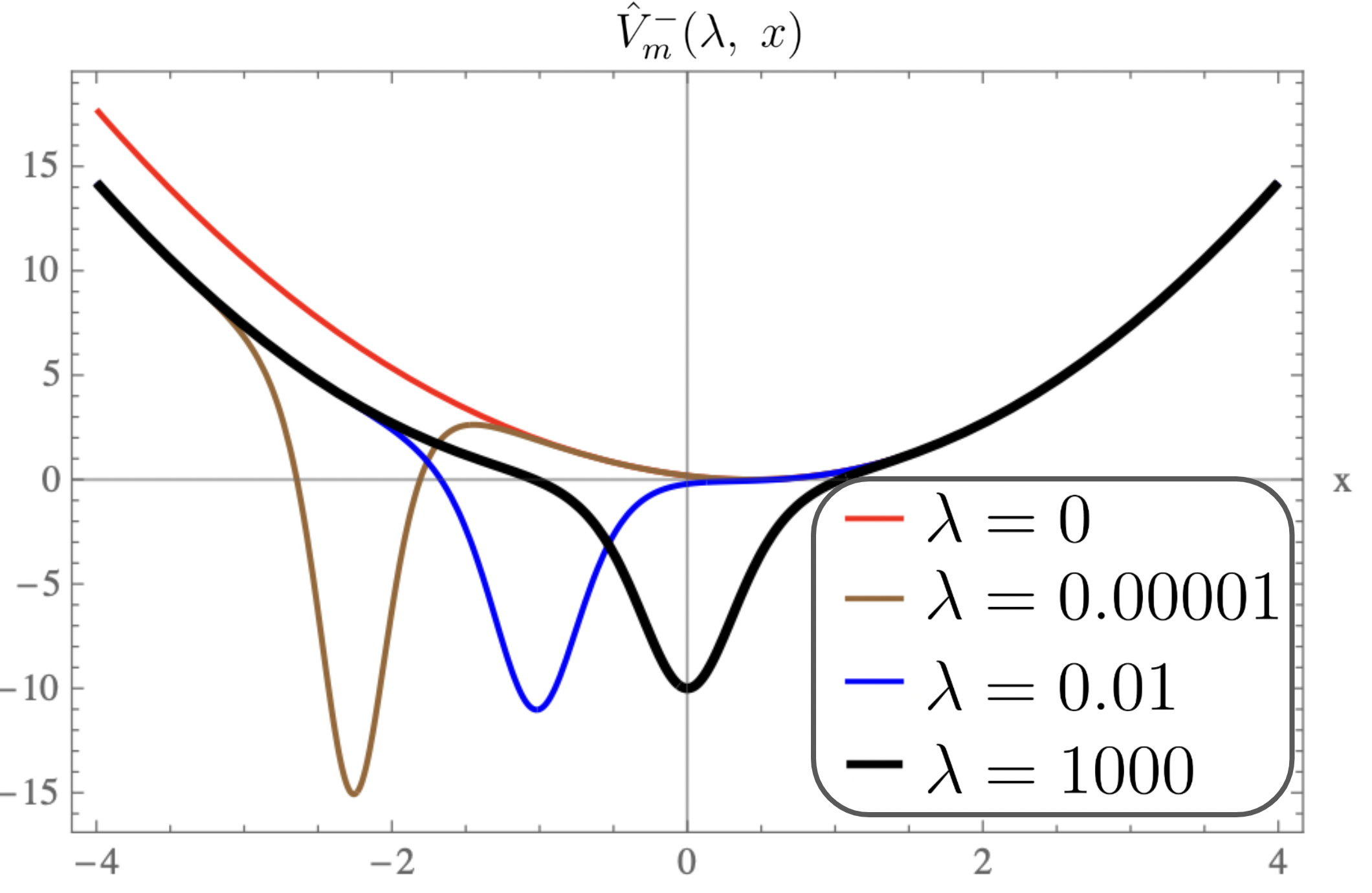
(a) Plot of $\hat{V}^{-}_{2}(\lambda,x)$ as a function of $x$ for positive $\lambda$.

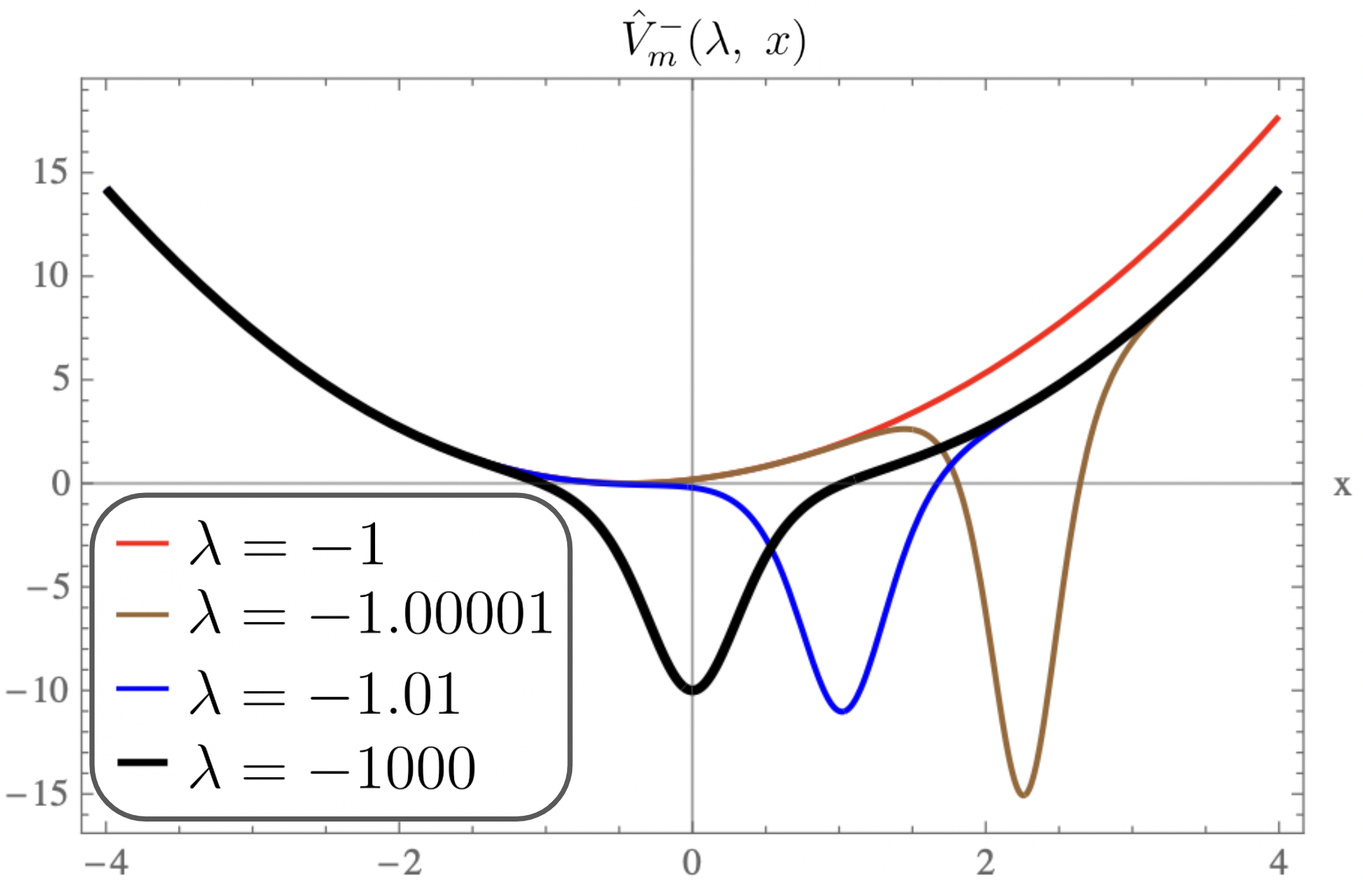
(b) Plot of $\hat{V}^{-}_{2}(\lambda,x)$ as a function of $x$ for negative $\lambda$.

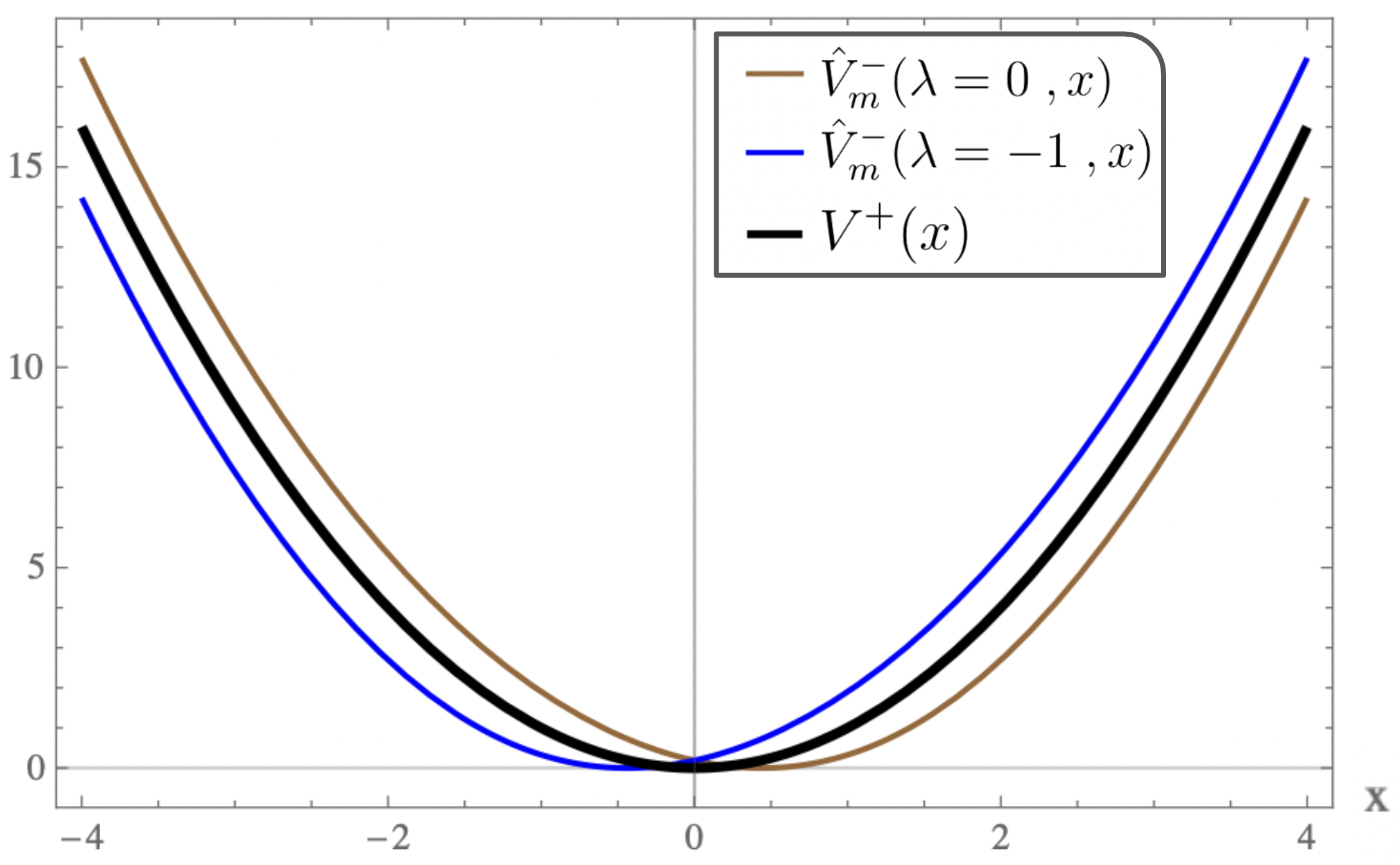
(c) Plot of Pursey $\hat{V}^{-}_{2}(0,x)$, AM $\hat{V}^{-}_{2}(-1,x)$ and $V^{+}(x)$ potential as a function of $x$

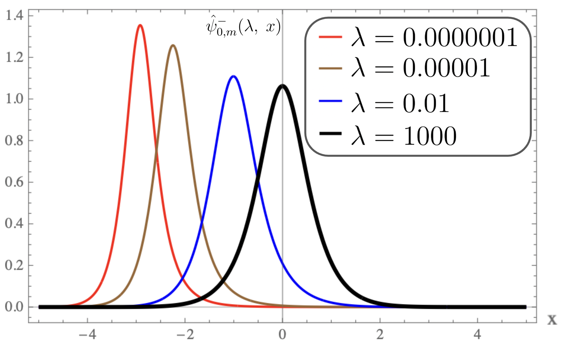
(d) Plot of Ground-state wavefunction $\hat{\psi}^{-}_{0,2}(\lambda,x)$ as a function of $x$ for various positive $\lambda$.

Figure 3: Plot of isospectral potential $\hat{V}^{-}_{2}(\lambda,x)$ and its ground state eigenfunction $\hat{\psi}^{-}_{0,2}(\lambda,x)$ as a function of $x$ for various $\lambda$ when $m=2$.

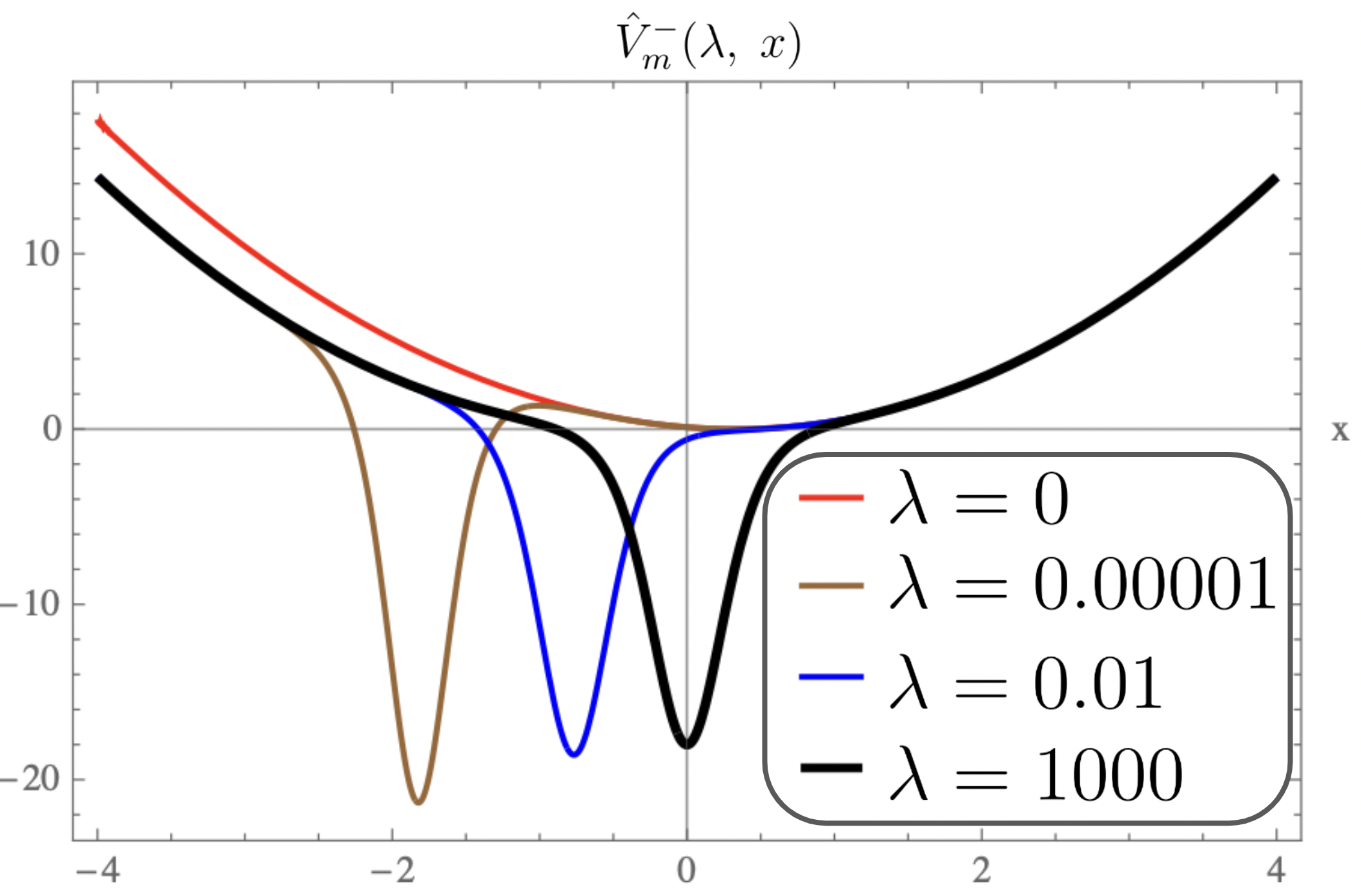
(a) Plot of $\hat{V}^{-}_{4}(\lambda,x)$ as a function of $x$ for positive $\lambda$.

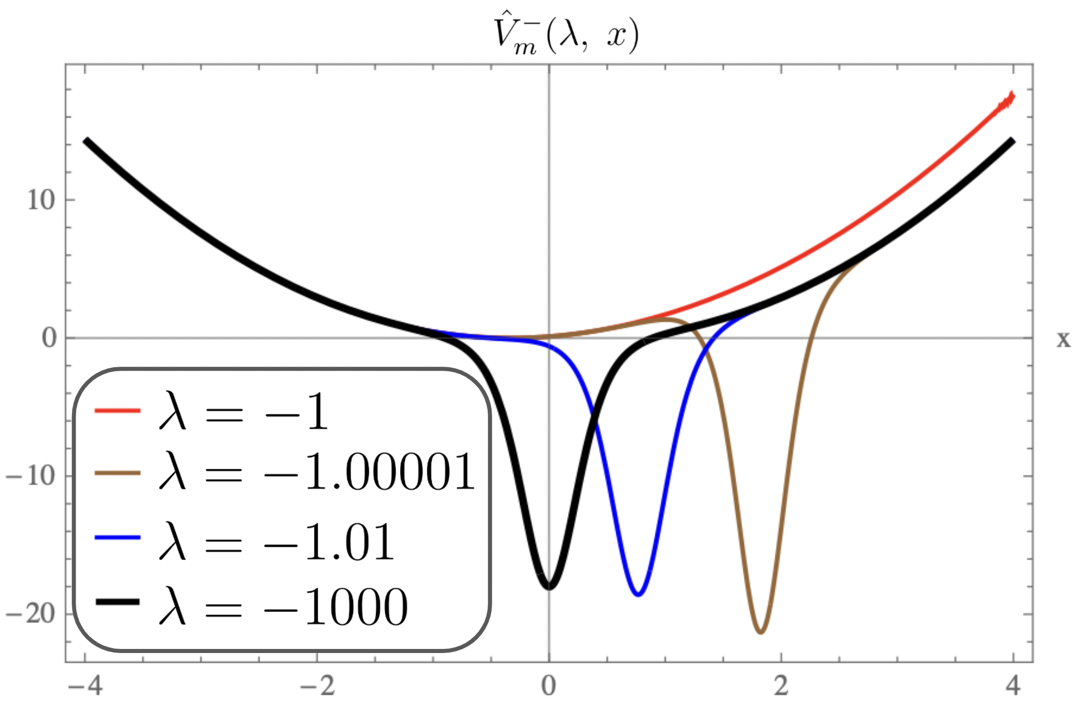
(b) Plot of $\hat{V}^{-}_{4}(\lambda,x)$ as a function of $x$ for negative $\lambda$.

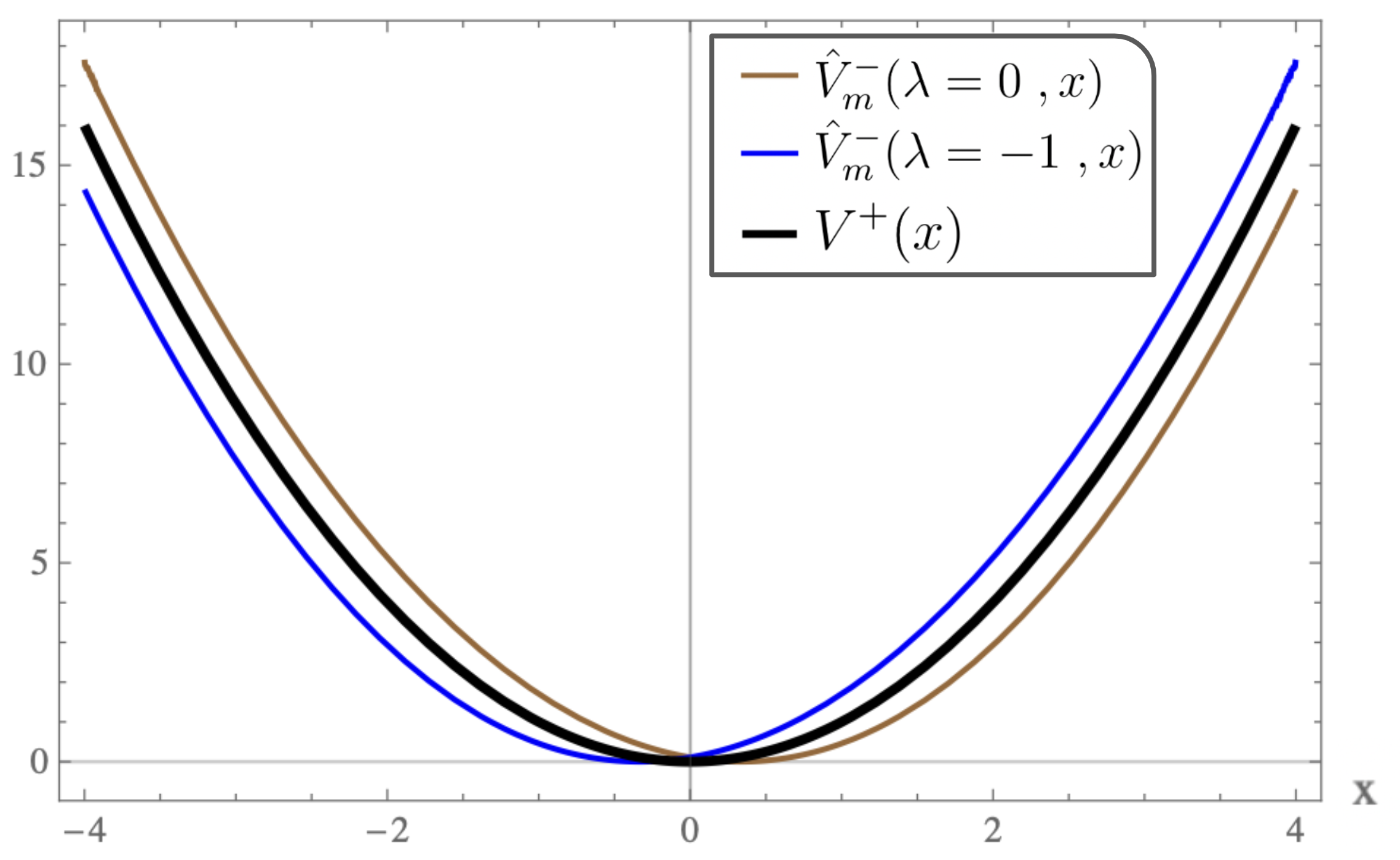
(c) Plot of Pursey $\hat{V}^{-}_{4}(0,x)$, AM $\hat{V}^{-}_{4}(-1,x)$ and $V^{+}(x)$ potential as a function of $x$

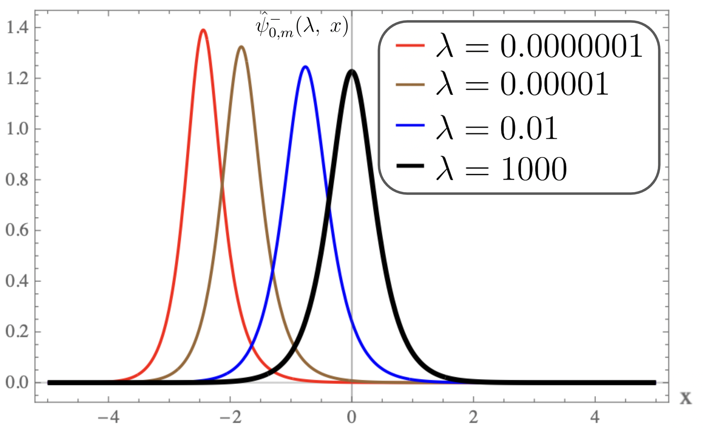
(d) Plot of Ground-state wavefunction $\hat{\psi}^{-}_{0,4}(\lambda,x)$ as a function of $x$ for various positive $\lambda$.

Figure 4: Plot of isospectral potential $\hat{V}^{-}_{4}(\lambda,x)$ and its ground state eigenfunction $\hat{\psi}^{-}_{0,4}(\lambda,x)$ as a function of $x$ for various $\lambda$ when $m=4$.

4 One parameter family of REHO potentials

The One parameter ($\lambda$) family of strictly isospectral potentials corresponding to $V^{-}_{m}(x)$ are easily obtained using (11-12) as

$$\hat{V}^{-}_{m}(\lambda,x)=V^{-}_{m}(x)-2\frac{d^{2}}{dx^{2}}\ln\left[\mathcal{I}_{m}(x)+\lambda\right],$$ (24)

where the integral $\mathcal{I}_{m}(x)$ is calculated using (18) as

$$\mathcal{I}_{m}(x)=\left(\frac{2^{m}m!}{\sqrt{\pi}}\right)\int^{x}_{-\infty}\left[\frac{e^{-\frac{{x^{\prime}}^{2}}{2}}}{\mathcal{H}_{m}(x^{\prime})}\right]^{2}dx^{\prime}.$$ (25)

The expressions for $\mathcal{I}_{m}(x)$ and $\hat{V}^{-}_{m}(\lambda,x)$ for $m$ equal to $0,\;2\text{ and }4$ are given in table-2 and table-3 respectively in terms of the error function $\text{erf}(x)$ defined as

$$\text{erf}(x)=1-\text{erfc}(x),\qquad\text{erfc}(x)=\frac{2}{\sqrt{\pi}}\int^{\infty}_{x}e^{-t^{2}}dt\,.$$

The normalized ground state wave function $\hat{\psi}^{-}_{0,m}(\lambda,x)$ is obtained using (11), (18) and (25) as

$$\hat{\psi}^{-}_{0,m}(\lambda,x)=\sqrt{\lambda(1+\lambda)}\;\frac{\psi^{-}_{0,m}(x)}{\mathcal{I}_{m}(x)+\lambda}\,.$$ (26)

m	$y^{m}_{n+1}(x),\qquad n=0,1,2\cdots$	$\mathcal{I}_{m}(x)$
0	$H_{n+1}(x)$	$\frac{1}{2}(\text{erf}(x)+1)$
2	$2\left(2x^{2}+1\right)H_{n+1}(x)+8xH_{n}(x)$	$\frac{1}{2}\left(\text{erf}(x)+\frac{2e^{-x^{2}}x}{\sqrt{\pi}\left(2x^{2}+1\right)}+1\right)$
4	$4\left(4x^{4}+12x^{2}+3\right)H_{n+1}(x)+\left(64x^{3}+96x\right)H_{n}(x)$	$\frac{1}{2}\left(\text{erf}(x)+\frac{2e^{-x^{2}}x\left(2x^{2}+5\right)}{\sqrt{\pi}\left(4\left(x^{2}+3\right)x^{2}+3\right)}+1\right)$

Table 2: Exceptional Hermite polynomials $y^{m}_{n+1}$ and $\mathcal{I}_{m}(x)$ for different $m$.

m	$\hat{V}^{-}_{m}(\lambda,x)$
0	$x^{2}-2+\frac{e^{-2x^{2}}\left(8\sqrt{\pi}e^{x^{2}}x(\text{erf}(x)+2\lambda+1)+8\right)}{\pi(\text{erf}(x)+2\lambda+1)^{2}}$
2	$x^{2}-2+\frac{8\left(\pi e^{2x^{2}}\left(2x^{2}-1\right)(\text{erf}(x)+2\lambda+1)^{2}+6\sqrt{\pi}e^{x^{2}}x(\text{erf}(x)+2\lambda+1)+4\right)}{\pi e^{2x^{2}}\left(2x^{2}+1\right)^{2}(\text{erf}(x)+2\lambda+1)^{2}+4\sqrt{\pi}e^{x^{2}}\left(2x^{3}+x\right)(\text{erf}(x)+2\lambda+1)+4x^{2}}$
4	$x^{2}-2+\frac{16\left(\pi e^{2x^{2}}\left(8x^{6}+12x^{4}+18x^{2}-9\right)(\text{erf}(x)+2\lambda+1)^{2}+16\sqrt{\pi}e^{x^{2}}x\left(x^{4}+x^{2}+3\right)(\text{erf}(x)+2\lambda+1)+4\left(2x^{4}+x^{2}+8\right)\right)}{\left(\sqrt{\pi}e^{x^{2}}\left(4\left(x^{2}+3\right)x^{2}+3\right)(\text{erf}(x)+2\lambda+1)+2x\left(2x^{2}+5\right)\right)^{2}}$

Table 3: Expression of isospectral potential $\hat{V}^{-}_{m}(x)$ for different $m$.

The normalized excited states eigenfunction of $\hat{V}^{-}_{m}(\lambda,x)$, using (12) are given by

$$\hat{\psi}^{-}_{n+1,m}(\lambda,x) =\frac{1}{E^{-}_{n+1,m}}\hat{A}^{\dagger}A\psi^{-}_{n+1,m}(x),\qquad n=0,1,2,\cdots,$$ (27)

$$=\frac{e^{-\frac{x^{2}}{2}}}{\sqrt{2(n+m+1)2^{n}n!\sqrt{\pi}}}\left(\frac{y^{m}_{n+1}(x)}{\mathcal{H}_{m}(x)}+H_{n}(x)\frac{d}{dx}\ln\left[\mathcal{I}_{m}(x)+\lambda\right]\right)$$

and

$$\hat{A}^{\dagger}=-\frac{d}{dx}-\frac{d}{dx}\ln\left[\frac{\psi^{-}_{0,m}(x)}{\mathcal{I}_{m}(x)+\lambda}\right],\qquad A=\frac{d}{dx}-\frac{d}{dx}\ln[\psi^{-}_{0,m}(x)].$$

The expression of $\hat{\psi}^{-}_{n+1,m}(x)$ for $m$ equal to $0,\;2\text{ and }4$ are tabulated in table-4 . As mentioned above, the spectra of $\hat{H}^{-}_{m}$, defined using (13), is strictly isospectral to $H^{-}_{m}$ spectra and is given by Eq. (20).

m	$\hat{\psi}^{-}_{n+1,m}(\lambda,x),\qquad n=0,1,2,\cdots$
0	$\frac{e^{-\frac{x^{2}}{2}}}{\sqrt{2(n+1)2^{n}n!\sqrt{\pi}}}\left(\frac{y^{0}_{n+1}(x)}{1}+\frac{2H_{n}(x)}{e^{x^{2}}\sqrt{\pi}(\text{erf}(x)+2\lambda+1)}\right)$
2	$\frac{e^{-\frac{x^{2}}{2}}}{\sqrt{2(n+3)2^{n}n!\sqrt{\pi}}}\left(\frac{y^{2}_{n+1}(x)}{4x^{2}+2}+\frac{4H_{n}(x)}{\left(2x^{2}+1\right)\left(\sqrt{\pi}e^{x^{2}}\left(2x^{2}+1\right)(\text{erf}(x)+2\lambda+1)+2x\right)}\right)$
4	$\frac{e^{-\frac{x^{2}}{2}}}{\sqrt{2(n+5)2^{n}n!\sqrt{\pi}}}\left(\frac{y^{4}_{n+1}(x)}{16x^{4}+48x^{2}+12}+\frac{48H_{n}(x)}{\sqrt{\pi}e^{x^{2}}\left(4\left(x^{2}+3\right)x^{2}+3\right)^{2}(\text{erf}(x)+2\lambda+1)+2x\left(8x^{6}+44x^{4}+66x^{2}+15\right)}\right)$

Table 4: Expression of excited state wavefunction $\hat{\psi}^{-}_{n+1,m}(x)$ for different $m$.

For $m$ equal to $0,\;2\text{ and }4$, the plots of the strictly isospectral potentials for positive and negative $\lambda$ as a function of $x$ are shown in Fig-(2.a, 3.a, 4.a) and Fig-(2.b, 3.b, 4.b) respectively. Pursey and Abraham-Moses potential plots as a function of $x$ are shown in Fig-(2.c, 3.c, 4.c). The ground-state wavefunction plots as a function of $x$ for various $\lambda$ are shown in Fig-(2.d, 3.d, 4.d). From the figures one observes that the eigen functions and the strictly isospectral potentials become sharper with increasing $m$. In the limit $\lambda$ approaching to $\pm\infty$ the potential $\hat{V}^{-}_{m}(\lambda,\;x)$ approaches to $V^{-}_{m}(x)$. Also notice that the potential starts developing a minimum when $\lambda$ decreases from $\infty$ to zero and the attractive potential well shifts towards $-\infty$ and finally vanishes when $\lambda$ equals zero. There is a loss of bound state and the corresponding potential is called the Pursey potential $V^{P}_{m}(x)$. An analogous situation occurs in the limit $\lambda=-1$ and the potential is called the Abraham-Moses potential $V^{AM}_{m}(x)$.

4.1 The Pursey and The Abraham-Moses Potentials

The Pursey and The Abraham-Moses Potentials are obtained from (27) by substituting $\lambda=0$ and $\lambda=-1$ respectively. In this case as mentioned above, one looses a bound state and the spectrum is identical to that of $H^{+}$, i.e.

$$\hat{E}^{P}_{n,m}=\hat{E}^{AM}_{n,m}=E^{+}_{n,m}\,,$$

where

$$E^{+}_{n,m}=2(n+m+1),\qquad n=0,1,2,3,\cdots$$

The normalized eigenfunctions of $\hat{V}^{P}_{m}(x)$ are given by

$$\hat{\psi}^{P}_{n,m}(x) =\frac{1}{E^{-}_{n+1,m}}\left(-\frac{d}{dx}-\frac{d}{dx}\ln\left[\frac{\psi^{-}_{0,m}(x)}{\mathcal{I}_{m}(x)}\right]\right)A\psi^{-}_{n+1,m}(x),\qquad n=0,1,2,\cdots,.$$ (28)

Similarly, the normalized eigenfunctions of $\hat{V}^{AM}_{m}(x)$ is given by

$$\hat{\psi}^{AM}_{n,m}(x) =\frac{1}{E^{-}_{n+1,m}}\left(-\frac{d}{dx}-\frac{d}{dx}\ln\left[\frac{\psi^{-}_{0,m}(x)}{\mathcal{I}_{m}(x)-1}\right]\right)A\psi^{-}_{n+1,m}(x),\qquad n=0,1,2,\cdots,.$$ (29)

The expression of $\hat{\psi}^{P}_{n,m}(x)$ and $\hat{\psi}^{AM}_{n,m}(x)$ for $m$ equal to $0,\;2\text{ and }4$ are obtained from table-4 by substituting $\lambda$ equal to $0$ and $-1$ respectively.
The ground state wavefunction plot for Pursey and AM potentials for various $m$ are shown in figure-5.b and transition in wavefunction shape as $\lambda$ approaches zero is shown in figure-5.a.

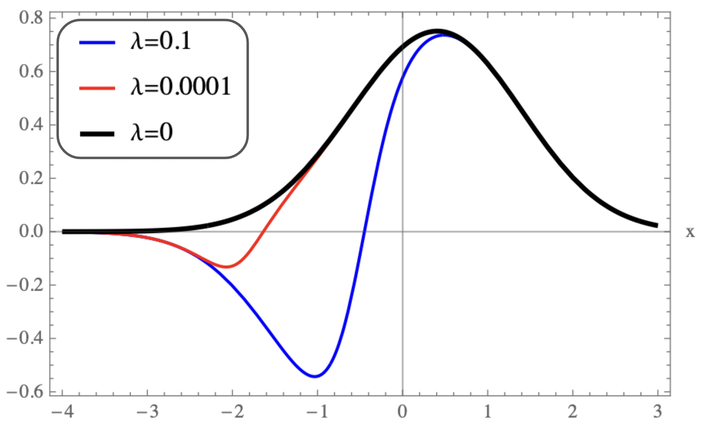
(a) Plot of first excited state eigenfunction $\hat{\psi}^{-}_{1,2}(\lambda,\;x)$ corresponding to potential $\hat{V}^{-}_{2}(\lambda,x)$ as a function of $x$ when $\lambda$ approaches 0.

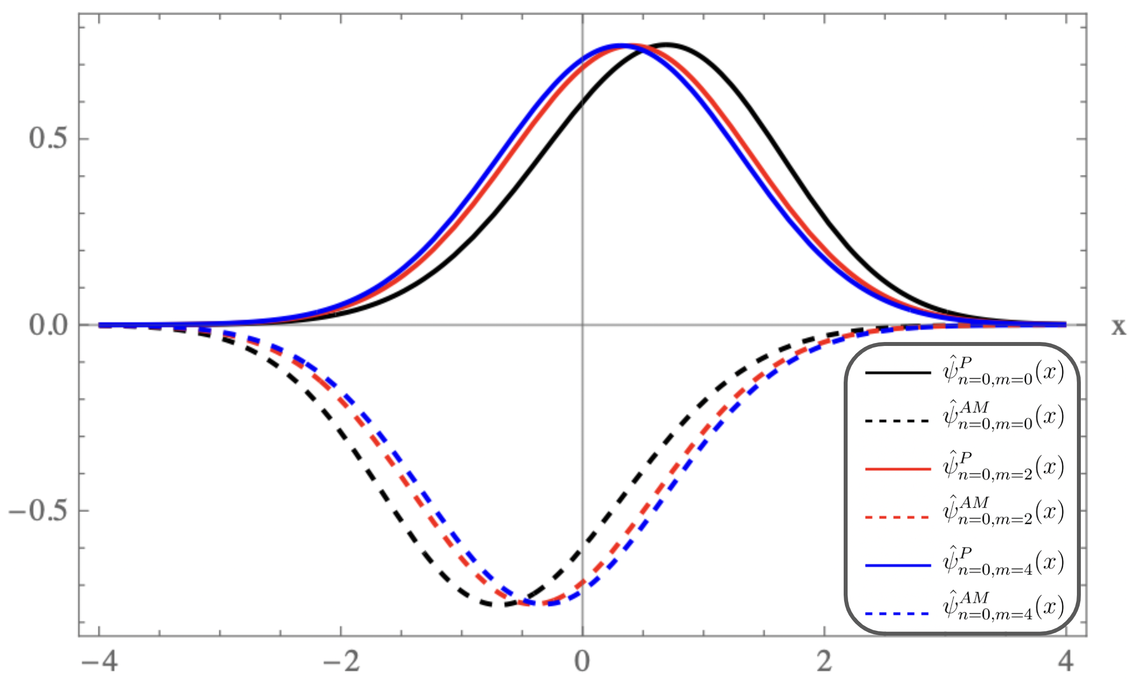
(b) Plot of ground state wavefunction of Pursey and AM potentials as a function of $x$ when $m=0$ (Black curve), $m=2$(Red curve) and $m=4$(Blue curve).

Figure 5: Dashing curve represents Pursey eigenfunction and dashed curve represents the AM eigenfunction.

5 Calculation of Uncertainty $\Delta x\Delta p$

The Heisenberg Uncertainty relation for position, $x$, and momentum, $p$, is defined as

$$\Delta x\Delta p=\sqrt{\left(<x^{2}>\;-\;<x>^{2}\right)\;\left(<p^{2}>\;-\;<p>^{2}\right)},$$ (30)

where, the angle bracket, $<>$, represents expectation value in a given wavefunction basis.

5.1 Uncertainty relation for REHO potential

For the REHO potentials the expectation value of the position, $x$, and the momentum, $p$, in the ground as well as the excited states is zero as the integrand is an odd function in the calculation of $<x>$ while the expectation value of $<p>$ is zero since the eigenfunctions are real. The uncertainty relation therefore takes the simpler form $\Delta x\Delta p=\sqrt{<x^{2}><p^{2}>}$

The expectation values and hence the uncertainty values can be calculated by using Eqs. (18). It is observed that $\Delta x=\Delta p$ for $m=0$ but the same is not true for $m\neq 0$. The uncertainty values for $m=0,1,2$ and $n=-1,0,1$ (i.e. ground, first and second excited states) are shown in table-5.

m	$n=-1$	$n=0$	$n=1$
0	$0.5$	$1.5$	$2.5$
2	$\approx 0.5172$	$\approx 1.554$	$\approx 2.3412$
4	$\approx 0.5212$	$\approx 1.6152$	$\approx 2.2102$

Table 5: Uncertainty relation $\Delta x\Delta p$ for potential $V^{-}_{m}(x)$ in ground state, first excited state and second excited state for $m$ equal to $0,\;2,\text{ and }4$.

It can be seen from figure-6.a that for the ground state, the uncertainty value increases as $m$ increases from $0$ and then flattens out around $m=10$. On the other hand, in the different excited states the Uncertainty values show peculair behaviour. In particular, while it decreases with increasing $m$ for any given even excited states but it increases with increasing $m$ for any given odd excited states. This peculiar behaviour in the uncertainty may be attributed to the even and odd degree of exceptional Hermite polynomials for a given $n$. The figure-6.b shows the variation of uncertainty with different excite states for $m$ equal to 0, 8 and 52.

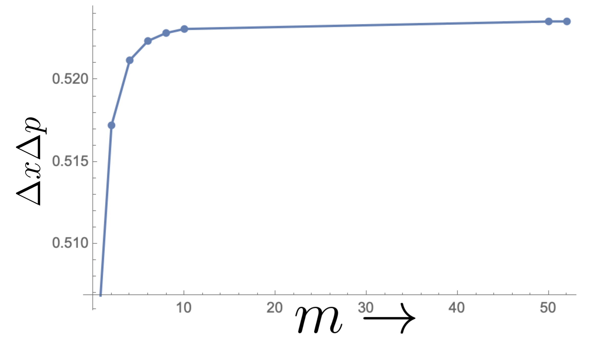
(a) Uncertainty at ground state for versus $m$.

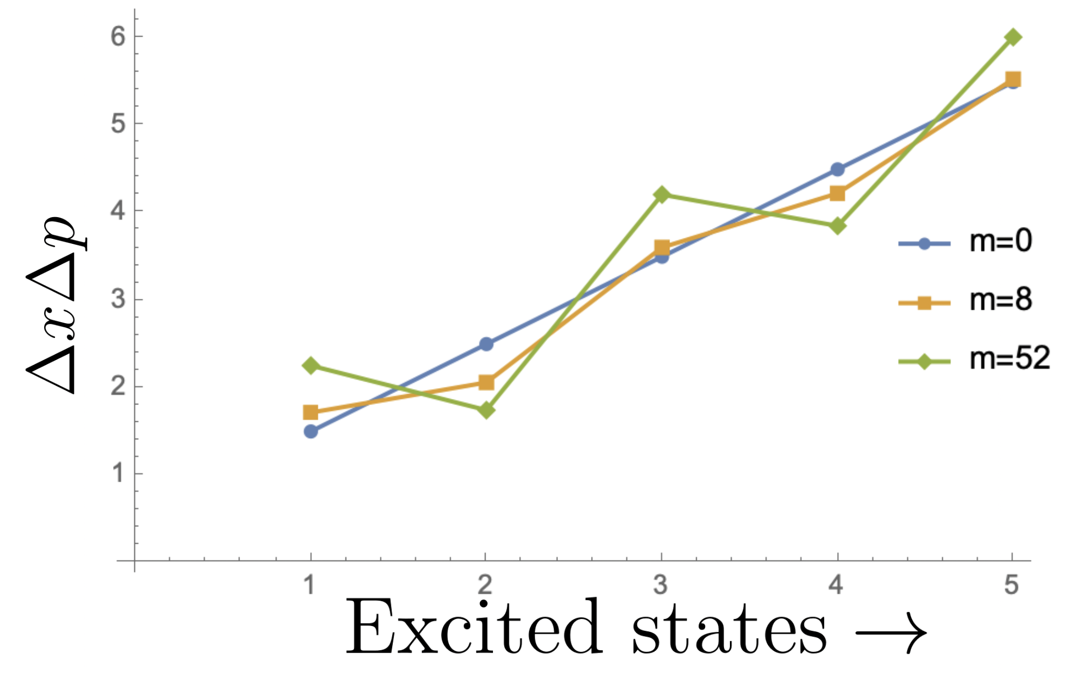
(b) Uncertainty at different excited state for $m$ equal to 0, 8 and 52.

Figure 6: Uncertainty trends with increasing $m$ and $n$.

5.2 Uncertainty relation for one parameter family of REHO potential

The expectation value of momentum, $<p>$, is again zero as the eigenfunctions are real. The uncertainty in $\Delta p$ is, therefore, $\sqrt{<p^{2}>}$. The expectation values of $x$, $x^{2}$ for various values of $m$ and $\lambda$ are given in Appendix A. The uncertainty relation at ground-state for various values of $m$ and $\lambda$ is given in table-6.

m/ $\lambda=$	$1\times 10^{-12}$	$1\times 10^{-8}$	$1\times 10^{-5}$	$1\times 10^{-3}$	$1\times 10^{-1}$	$1\times 10^{2}$
0	$\approx 0.5202$	$\approx 0.5281$	$\approx 0.5367$	$\approx 0.5590$	$\approx 0.5455$	$\approx 0.5000$
2	$\approx 0.5223$	$\approx 0.5270$	$\approx 0.5285$	$\approx 0.5266$	$\approx 0.5193$	$\approx 0.5172$
4	$\approx 0.5228$	$\approx 0.5252$	$\approx 0.5246$	$\approx 0.5232$	$\approx 0.5215$	$\approx 0.5212$

Table 6: Uncertainty relation $\Delta x\Delta p$ for potential $\hat{V}^{-}_{m}(\lambda,x)$ in ground state for $m$ equal to $0,\;2,\text{ and }4$.

When the values of $\lambda(>0)$ in the table-6 are replaced by $-|\lambda+1|$ the uncertainty relation $\Delta x\Delta p$ remains unchanged and it corresponds to the Abraham Moses potential. The plot of uncertainty versus $\lambda$ for $m=0$ and $m=2$ is shown in figure-7.a and 7.b respectively. The peak of uncertainty curve rapidly moves towards origin with increasing $m$.

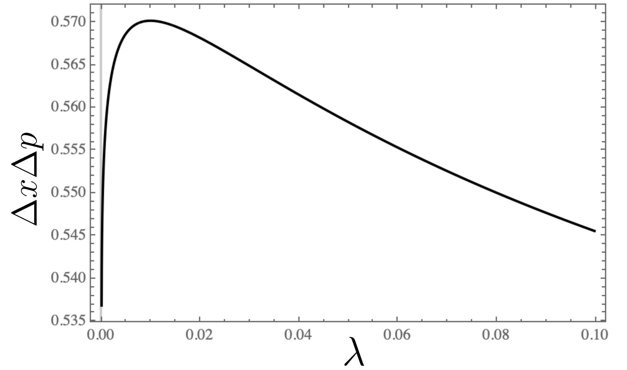
(a) m=0 case.

(b) m=2 case.

Figure 7: Uncertainty versus positive $\lambda$ graph for $m=0$ and $m=2$.

5.2.1 Uncertainty relations for Pursey and Abraham Moses Potentials

The expectation value of $x$ and $x^{2}$ are calculated in Appendix C for various values of $m$. It is interesting to note that the expectation value of $x$ is equal and opposite in the case of the Pursey and the AM Potentials while the expectation value of $x^{2}$ and $p^{2}$ is the same in both the cases.

m/n	0	1	2	3	10
0	$\approx 0.50184$	$\approx 1.4879$	$\approx 2.4894$	$\approx 3.4905$	$\approx 10.4947$
2	$\approx 0.50015$	$\approx 1.4990$	$\approx 2.4984$	$\approx 3.4980$	$\approx 10.4977$
4	$\approx 0.50004$	$\approx 1.4997$	$\approx 2.4994$	$\approx 3.4992$	$\approx 10.4987$

Table 7: Uncertainty relation $\Delta x\Delta p$ for potential $\hat{V}^{P}_{m}(x)$ or $\hat{V}^{AM}_{m}(x)$ for various $n$ and for $m$ equal to $0,\;2,\text{ and }4$.

As a result the uncertainty value corresponding to a given $m$ is the same for the Pursey and the AM potentials. The uncertainty value for the Pursey and the AM potentials at the ground and the different excited-states is given in table-7. The uncertainty decreases at ground state with increasing $m$ and becomes asymptotic to $0.5$. On contrast it is seen that uncertainty is lesser than QHO ($m=0$) uncertainty for excited states.

6 Summary and discussion

In this manuscript, we consider the rationally extended one dimensional harmonic oscillator potential associated with exceptional $X_{m}$-Hermite polynomials. Unlike the one dimensional oscillator, for nonzero $m$, while the energy gap between the excited states is $2$ units, the energy gap between the groundstate and first excited state is $m+1$. Using the idea of SQM, we obtained one parameter ($\lambda$) family of strictly isospectral potentials corresponding to the REHO potential as well as the corresponding eigenfunctions. As a special case, as $\lambda$ approaches $0$ or $-1$, we obtained the rationally extended Pursey and the AM potentials respectively as well as their eigenfunctions. Further, we calculated the Heisenberg uncertainty relations $\Delta x\Delta p$ for the REHO and as well as the corresponding strictly isopectral one parameter ($\lambda$) family of potentials. In addition, we also calculated the uncertainity relation for the corresponding Pursey and AM potentials. In the case of the REHO, we showed that the ground state uncertainity increases as $m$ increases. In the case of the strictly isospectral one parameter family of potentials, one finds that the uncertainty relation depends on $m$ as well as $\lambda$. Remarkably, we find that for any $m$, the uncertainty relation is the same for the Pursey and the AM potentials.

There are several open problems. For example, In this paper we have only studied the potentials with even codimension $m$ and obtained the corresponding strictly isospectral one parameter family. Can one similarly obtain the corresponding one parameter family of potentials in case the codimension $m$ is odd. Further, apart from the one dimensional oscillator, are there other rationally extended potentials for which the eigenfunctions can be expressed in terms of exceptional Hermite polynomials? Another obvious question is whether there are exceptional Legendre polynomials and if yes can one discover new potentials whose eigenfunctions can be expressed in terms of exceptional Legendre polynomials? We hope to study some of these problems in coming days.

Acknowledgements
AK is gratefel to Indian National Science Academy (INSA) for awarding INSA Honarary Scientist position at Savitribai Phule Pune University. One of us (RK) is grateful to Ian Marquette for useful comments.

Appendix A. Expectation value of $x$ and $x^{2}$ for one parameter family of REHO
The expectation value of $x$ and $x^{2}$ for various values of positive $\lambda$ are calculated using (26) as:

$$<x>=\begin{cases}\approx-3.0028\|_{m=0}\;\approx-2.2259\|_{m=2}\;\approx-1.8057\|_{m=4}&\text{, when $\lambda=0.00001$}\\ \approx-2.1553\|_{m=0}\;\approx-1.4304\|_{m=2}\;\approx-1.1187\|_{m=4}&\text{, when $\lambda=0.001$}\\ \approx-0.9133\|_{m=0}\;\approx-0.5202\|_{m=2}\;\approx-0.3955\|_{m=4}&\text{, when $\lambda=0.1$}\\ \approx-0.0039\|_{m=0}\;\approx-0.0022\|_{m=2}\;\approx-0.0016\|_{m=4}&\text{, when $\lambda=100$}\\ \approx-0.0004\|_{m=0}\;\approx-0.0002\|_{m=2}\;\approx-0.0002\|_{m=4}&\text{, when $\lambda=1000$}\\ \end{cases}$$

When the values of $\lambda(>0)$ in the above table are replaced by $-|\lambda+1|$ the magnitude of the values of $x$ remain unchanged but the sign reverses.

$$<x^{2}>=\begin{cases}\approx 9.1024\|_{m=0}\;\approx 5.0384\|_{m=2}\;\approx 3.3276\|_{m=4}&\text{, when $\lambda=0.00001$}\\ \approx 4.8071\|_{m=0}\;\approx 2.1621\|_{m=2}\;\approx 1.3309\|_{m=4}&\text{, when $\lambda=0.001$}\\ \approx 1.2338\|_{m=0}\;\approx 0.4198\|_{m=2}\;\approx 0.2446\|_{m=4}&\text{, when $\lambda=0.1$}\\ \approx 0.5000\|_{m=0}\;\approx 0.1556\|_{m=2}\;\approx 0.0896\|_{m=4}&\text{, when $\lambda=100$}\\ \approx 0.5\|_{m=0}\;\approx 0.1556\|_{m=2}\;\approx 0.0896\|_{m=4}&\text{, when $\lambda=1000$}\\ \end{cases}$$

When the values of $\lambda(>0)$ in the above table are replaced by $-|\lambda+1|$ the expectation values of $x^{2}$ remains unchanged. Similarly, the expectation value of $p^{2}$ can be calculated.

Appendix B. Expectation value of $x$ and $x^{2}$ for Puresey and Abraham Moses Potentials
The expectation value and uncertainty relation can be calculated from (28) and (29).

The expectation value of $x$ and $x^{2}$ for various values of $m$ are as follows:

$$<x>=\begin{cases}\approx 0.6386\|_{\text{Pursey}}\;\approx-0.6386\|_{\text{AM}}&\text{, when $m=0$}\\ \approx 0.3928\|_{\text{Pursey}}\;\approx-0.3928\|_{\text{AM}}&\text{, when $m=2$}\\ \approx 0.3087\|_{\text{Pursey}}\;\approx-0.3087\|_{\text{AM}}&\text{, when $m=4$}\\ \end{cases}$$

$$<x^{2}>=\begin{cases}\approx 0.9043\|_{\text{Pursey}}\;\approx 0.9043\|_{\text{AM}}&\text{, when $m=0$}\\ \approx 0.6539\|_{\text{Pursey}}\;\approx 0.6539\|_{\text{AM}}&\text{, when $m=2$}\\ \approx 0.5952\|_{\text{Pursey}}\;\approx 0.5952\|_{\text{AM}}&\text{, when $m=4$}\\ \end{cases}$$

References

- [1] Fred Cooper, Avinash Khare, and Uday Sukhatme. Supersymmetry and quantum mechanics. Physics Reports, 251(5-6):267–385, 1995.
- [2] ZS Agranovich and Vladimir Aleksandrovich Marchenko. The inverse problem of scattering theory. Courier Dover Publications, 2020.
- [3] Khosrow Chadan and Pierre C Sabatier. Inverse problems in quantum scattering theory. Springer Science & Business Media, 2012.
- [4] George L Lamb Jr. Elements of soliton theory. New York, page 29, 1980.
- [5] Philip G Drazin and Robin Stanley Johnson. Solitons: an introduction, volume 2. Cambridge university press, 1989.
- [6] Michael Martin Nieto. Relationship between supersymmetry and the inverse method in quantum mechanics. Physics Letters B, 145(3-4):208–210, 1984.
- [7] RD Amado. Phase-equivalent supersymmetric quantum-mechanical partners of the coulomb potential. Physical Review A, 37(7):2277, 1988.
- [8] DL Pursey. Isometric operators, isospectral hamiltonians, and supersymmetric quantum mechanics. Physical Review D, 33(8):2267, 1986.
- [9] PB Abraham and HE Moses. Changes in potentials due to changes in the point spectrum: anharmonic oscillators with exact solutions. Physical Review A, 22(4):1333, 1980.
- [10] G Darboux. On a proposition relative to linear equations. arXiv preprint physics/9908003, 1999.
- [11] Satoru Odake and Ryu Sasaki. Krein–adler transformations for shape-invariant potentials and pseudo virtual states. Journal of Physics A: Mathematical and Theoretical, 46(24):245201, 2013.
- [12] Avinash Khare and Uday Sukhatme. Phase-equivalent potentials obtained from supersymmetry. Journal of Physics A: Mathematical and General, 22(14):2847, 1989.
- [13] Wai-Yee Keung, Uday P Sukhatme, Qinmou Wang, and Tom D Imbo. Families of strictly isospectral potentials. Journal of Physics A: Mathematical and General, 22(21):L987, 1989.
- [14] David Gómez-Ullate, Niky Kamran, and Robert Milson. An extended class of orthogonal polynomials defined by a sturm–liouville problem. Journal of Mathematical Analysis and Applications, 359(1):352–367, 2009.
- [15] David Gomez-Ullate, Niky Kamran, and Robert Milson. Exceptional orthogonal polynomials and the darboux transformation. Journal of Physics A: Mathematical and Theoretical, 43(43):434016, 2010.
- [16] David Gomez-Ullate, Niky Kamran, and Robert Milson. On orthogonal polynomials spanning a non-standard flag. Contemp. Math, 563:51–71, 2012.
- [17] Bikashkali Midya and Barnana Roy. Exceptional orthogonal polynomials and exactly solvable potentials in position dependent mass schrödinger hamiltonians. Physics Letters A, 373(45):4117–4122, 2009.
- [18] Choon-Lin Ho. Dirac (-pauli), fokker–planck equations and exceptional laguerre polynomials. Annals of Physics, 326(4):797–807, 2011.
- [19] Rajesh Kumar Yadav, Avinash Khare, and Bhabani Prasad Mandal. The scattering amplitude for a newly found exactly solvable potential. Annals of Physics, 331:313–316, 2013.
- [20] Rajesh Kumar Yadav, Avinash Khare, and Bhabani Prasad Mandal. The scattering amplitude for rationally extended shape invariant eckart potentials. Physics Letters A, 379(3):67–70, 2015.
- [21] C-L Ho, J-C Lee, and R Sasaki. Scattering amplitudes for multi-indexed extensions of solvable potentials. Annals of Physics, 343:115–131, 2014.
- [22] Rajesh Kumar Yadav, Nisha Kumari, Avinash Khare, and Bhabani Prasad Mandal. Group theoretic approach to rationally extended shape invariant potentials. Annals of Physics, 359:46–54, 2015.
- [23] Nisha Kumari, Rajesh Kumar Yadav, Avinash Khare, Bijan Bagchi, and Bhabani Prasad Mandal. Scattering amplitudes for the rationally extended pt symmetric complex potentials. Annals of Physics, 373:163–177, 2016.
- [24] Rajesh Kumar Yadav, Avinash Khare, Bijan Bagchi, Nisha Kumari, and Bhabani Prasad Mandal. Parametric symmetries in exactly solvable real and pt symmetric complex potentials. Journal of Mathematical Physics, 57(6):062106, 2016.
- [25] Nisha Kumari, Rajesh Kumar Yadav, Avinash Khare, and Bhabani Prasad Mandal. A class of exactly solvable rationally extended calogero–wolfes type 3-body problems. Annals of Physics, 385:57–69, 2017.
- [26] Rajesh Kumar Yadav, Avinash Khare, Nisha Kumari, and Bhabani Prasad Mandal. Rationally extended many-body truncated calogero–sutherland model. Annals of Physics, 400:189–197, 2019.
- [27] B Basu-Mallick, Bhabani Prasad Mandal, and Pinaki Roy. Quasi exactly solvable extension of calogero model associated with exceptional orthogonal polynomials. Annals of Physics, 380:206–212, 2017.
- [28] Suman Banerjee, Rajesh Kumar Yadav, Avinash Khare, Nisha Kumari, and Bhabani Prasad Mandal. Solutions of (1+ 1)-dimensional dirac equation associated with exceptional orthogonal polynomials and the parametric symmetry. arXiv preprint arXiv:2211.02557, 2022.
- [29] Arturo Ramos, Bijan Bagchi, Avinash Khare, Nisha Kumari, Bhabani Prasad Mandal, and Rajesh Kumar Yadav. A short note on “group theoretic approach to rationally extended shape invariant potentials”[ann. phys. 359 (2015) 46–54]. Annals of Physics, 382:143–149, 2017.
- [30] David Gómez-Ullate, Yves Grandati, and Robert Milson. Rational extensions of the quantum harmonic oscillator and exceptional hermite polynomials. Journal of Physics A: Mathematical and Theoretical, 47(1):015203, 2013.
- [31] Jonathan M Fellows and Robert A Smith. Factorization solution of a family of quantum nonlinear oscillators. Journal of Physics A: Mathematical and Theoretical, 42(33):335303, 2009.
- [32] Ian Marquette and Christiane Quesne. Two-step rational extensions of the harmonic oscillator: exceptional orthogonal polynomials and ladder operators. Journal of Physics A: Mathematical and Theoretical, 46(15):155201, 2013.
- [33] Rajesh Kumar Yadav, Suman Banerjee, Nisha Kumari, Avinash Khare, and Bhabani Prasad Mandal. One parameter family of rationally extended isospectral potentials. Annals of Physics, 436:168679, 2022.