Understanding the householder solar panel consumer: a Markovian Model and its Societal implications

Abstract

We propose a Markovian model to understand how Italy’s public sphere behaves on the green energy transition theme. The paper uses the example of solar photovoltaics as a point of reference. The adoption decision is assumed to be sequentially influenced by the network communication of each person or family and the payback period of the investment. We apply the model for a case study based on the evolution of residential PV systems in Italy over the 2006–2026 period. The baseline configuration of the model is calibrated based on the actual diffusion of residential PV in Italy from 2006 to 2020. The comprehensive analysis leads to a discussion of two interesting societal implications. (1) Cognitive biases such as hyperbolic discounting of individual future utility crucially influence inter-temporal green choices. (2) Individual green choices count for the effect that it has on the chances that other individuals will also make a choice, in turn abating other greenhouse gas emissions.

Keywords: green energy transition, solar photovoltaic, individual based modeling, ethics and mathematics, procrastination, Markovian model.
2020 Mathematics Subject Classification: 60K35, 91A16, 60J27.

1 Introduction

1.1 Motivation of the work and modelling framework

An original and exciting aspect of the present work is that it originates from the common desire of a group of Mathematicians and Philosophers to understand how Italy’s public sphere behaves on the theme of the Green Energy Transition (GET, henceforth). For the public sphere, here we mean individual people or families, simply agents hereafter. It is important to point out that in many areas of research with the term agents, one refers exclusively to individuals whose actions (also named controls) are the result of an optimization process. However, in [14], authors show that a Markovian-type modeling framework, i.e., a framework in which agents do not make rational decisions based on optimization rules, is more suitable to describe the public sphere’s behavior on the GET, where people occasionally question their-selves about the GET problem. This is also confirmed by the extensive literature on opinion dynamics in which the evolution of opinions in society is modeled through Markov chains; see, e.g., [37, 38, 38, 39, 40].
There is a growing acknowledgment in the literature and practice that, despite energy technology being available, and in many cases economically beneficial, other barriers prevent households’ widespread adoption of new green technologies (see, e.g., [28]). In particular, our discussions have mainly been focused on the following two elements: (1) the tendency of humans to mimic the behavior of other people; (2) the natural tendency of humans to procrastinate. Among the GET examples, we focus on the case of photovoltaic systems (PVs, henceforth), the primary motivation being the availability of a relatively significant sample of data; see Subsection 3.1. The present article provides conceptual and empirical results to better understand agent behavior in the solar photovoltaic market. It aims at answering the following research question: What does it play an essential role in the decision process for PVs?
The generation of electricity from PVs has played an essential role in the transition towards an energy system based on renewable energy ([19]). It thereby contributes to meeting the climate change mitigation scenario in which global temperature rise is kept within 1.5 degrees Celsius ([20]). Figure 1 displays Italy’s renewable electricity production by sources over 2006–2020. Several non-trivial elements are worth noting in the “Solar” time series. First, a change of regime around 2012. Second, an approximate exponential growth in each of the two periods. Figure 2, instead, displays the “Solar” decomposition among the following four categories: “Agriculture,” “Domestic,” “Services,” and “Industry,” with the “Domestic” one being our main focus (see the discussion above).

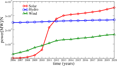
Figure 1: Evolution of Italy’s renewable electricity production by sources: “Solar” (red line), “Hydro” (blue line), “Wind” (green line) over 2006–2020. Data Source :  Terna Spa (https://www.terna.it).

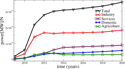
Figure 2: Evolution of Italy’s electricity production, source “Solar”, by categories: “Agriculture” (blue line), “Domestic” (black line), “Services” (red line), “Industry” (green line) over 2006–2020. Data Source :  GSE (https://www.gse.it/dati-e-scenari/statistiche).

In the present work, we consider two Markovian models; in particular, the second model is a refinement of the first one. In both models, a variable $X_{t}^{i}$ characterizes the state of each agent i, i$\in\{1,\ldots,N\}$, being $N$ the number of agents. A value of $X_{t}^{i}=C$ stands for “Carbon” and indicates that the individual has not decided on the theme of GET yet. She/he can be either agnostic to such a theme or prone to change her/his mind. For instance, she/he can be prone to mimicry, easily swayed by the behaviors of others in her/his social group, and attentive to social power and hierarchy. A value of $X_{t}^{i}=I$ stands for “Informed” and characterizes an agent that is fully informed on the benefits of PVs or that has developed a certain level of sensitivity to climate change and environmental issues. Finally, $X_{t}^{i}=G$ stands for “Green” and denotes the state of the individual that has installed the PVs. In the first model, we assume that each agent $i$ can only pass from the state “Carbon” to “Informed”, and from the state “Informed” to “Green”; the precise mechanism under which the transition takes place is described in Section 2. In the second model, more structure is added to the transition from the state “Informed” to the state “Green.” This additional structure hinges on the concept of procrastination, which means postponing into the future something that, from a subjective perspective, it would be rational to do earlier ([1]). We will remind some aspects relevant to the present work of GET and procrastination in Subsection 1.2, and refer to [14], Section 2, for a detailed presentation about the procrastination concept. More precisely, we add a state to the variable $X_{t}^{i}$ to capture such a behavior. The value $X_{t}^{i}=PL$ stands for “Planner”. It indicates an agent that plans to install the PVs soon because she/he has sufficient information on the benefits of PVs or has developed a certain level of sensitivity to climate change and environmental issues. When this happens, agent $i$ can only pass from “Informed” to “Planner” and then, as before, from “Planner” to “Green.” Again, the precise mechanism under which the transition occurs is described in Section 2. It is important to note that in both models, we assume, as predominantly done in behavioral economics, that the final transition from “Informed” to “Green” or from “Planner” to “Green” happens in response to a cost-benefit ratio. We assume that each agent makes the final choice of installing PVs based on benefits outweighing costs. More precisely, we assume that our agents first become an homo sustinens agents ([17]), and then (necessarily) homo economicus agents before making the transition to the state “Green”; see Table 3 in [17] for a nice overview of these two types of agents. Admittedly, one can construct a refinement of the second model in which some agents can pass from “Informed” to “Green,” but we leave this extension for future research (we will return to this point later). We also mention two other possible refinements that we would like to consider in the future. First, we desire to include the possibility that the transition from $I$ to $C$ occurs. In other words, we desire to include the mechanisms that cause an agent’s opinion to revert to the initial one. Another significant point would be the inclusion of bureaucratic obstacles to installations, such as slow installation and difficulty finding technical information. In the following subsection, we explain why GET can be considered an inter-temporal choice, in addition to the procrastination phenomena.

1.2 GET as an inter-temporal choice and the procrastination phenomena

Almost all energy transition decisions have an inter-temporal structure, in the sense that they imply an initial investment cost, both economic and bureaucratic, to reap benefits in the feature, in terms of lower energy consumption, through energy efficiency or the use of renewable energy sources (economically cheaper than fossil fuels). In particular, the choice about the adoption of the PV is a clear inter-temporal choice. Usually, the investment pays for itself over the years because the electricity produced with the PV has no variable costs, only fixed costs due to the maintenance of the facility. Not all individuals who have not adopted PV can be defined as procrastinators. Several factors may, in fact, explain the non-choice as rational: e.g., lack of capital and/or difficulties in accessing credit, epistemic obstacles (many people find it difficult to compare the different options available on the market), relational and/or administrative problems (not everyone lives in a semi-detached house, or in houses they own), miss-perception of risk, and so on. However, all those who have overcome these decision-making barriers and formed a clear preference for the PV purchase may end up trapped in a procrastination loop due to the inter-temporal structure of the green choice. In other words, it is not enough for an individual to develop a preference for a solar panel, as this decision may irrationally reverse itself as the time of purchase approaches. That is, when the discount rate of future utility changes from exponential to hyperbolic, and the value of the initial investment costs, previously judged lower than the value of the energy benefits to be reaped in the future, suddenly becomes higher. This reversal of preferences is obviously temporary and is normally accompanied by remorse, as in all cases of procrastination. There is a quite large understanding/acknowledgment that inducing people to form a green preference is the key to the energy transition (see [26]). We claim that this is insufficient, both to explain the data on PV adoption and to induce increases in green technology adoption rates because it does not take into account the traps of irrationality that accompany the implementation phase of green preferences.

1.3 The development of the PVs in Italy (see [14], Section 2)

This subsection briefly reviews the initiatives implemented by the Italian government to encourage the diffusion of PVs, henceforth) from 2005 until today. These initiatives are called “Conto Energia” (CE); each CE guarantees contracts with fixed conditions for 20 years for grid-connected PVs with at least 1kW of peak power. Local electricity providers are required by law to buy the electricity that is generated by PVs. The first CE started in 2005, and it was a net metering plan (“scambio sul posto”) designed for small PVs. The plan was meant to favor the direct use of self-produced electricity. Besides payment for each produced kWh of electricity, the consumer received additional rewards for directly consuming the self-generated energy. The CE2 was available to all PVs, but it was designed for larger plants with no or limited direct electricity self-consumption. The electricity produced was sold to the local energy supplier, for which the CE guarantees an additional Feed in Tariff (FiT, henceforth). It is important to mention that in each new version of the CE, the FiT was decreased (from 0.36 €/kWh in 2006 to 0.20 €/kWh in 2012). With the introduction of CE4 (2011) direct consumption was rewarded financially. The CE5, unlike the CE4, provided incentives based on the energy fed into the grid and a premium rate for self-consumed energy.

After the end of the fifth CE program, FiT and premium schemes were dropped, and a tax credit program was implemented in 2013. After six years, in 2019, a new incentive decree for photovoltaic systems (RES1) was reintroduced, reserved for systems with a capacity of more than 20 kW but not more than 1 MW. Subsidies are paid on the basis of net electricity produced and fed into the grid. The unit incentive varies according to the size of the plant. An incentive is provided for plants that replace asbestos or eternity roofing, and a bonus on self-consumption of energy (provided it is greater than 40% and the building is on a roof) is issued. For residential customers, a subsidized tax deduction is set at 50% instead of 36%.

However, in May 2020, the Italian government issued the “Revival Decree” (Decree Law 34/2020) in which a further increase to 110% was introduced. Depending on whether the installation is connected to energy-saving measures or not, the 110% tax deduction can be applied to the entire investment (max 2400 €/kW) or otherwise only to a part of it (max 1600 €/kW). In addition, the energy not consumed directly is transferred free of charge to the grid. In addition, the Revival Decree provides for the subsidized tax at 110% and also for the implementation of battery energy storage systems up to an amount of 1000 €/kWh. In addition, the Relaunch Decree provides for the subsidized tax at 110% also for the implementation of storage systems up to an amount of 1000 €/kWh.

Finally, an additional policy measure was introduced by the Ministerial Decree of September 16, 2020 which provides incentives for the configuration of collective self-consumption and renewable energy communities equal to 100 €/MWh and 110 €/MWh, respectively. The incentive lasts for 20 years, does not apply to plants exceeding a power of 200 kW, and has a duration of 60 days from the entry into force of the decree.

1.4 Related literature and our contribution

In his article, Gifford ([16]) proposes a framework to describe why humans are not taking action to prevent or ameliorate climate change. Energy inefficiency is a similarly complex and abstract problem to climate change. In particular, Gifford postulates the following seven “dragons” of inaction with regard to climate change: (1) “limited cognition,” (2) “ideologies,” (3) “dis-credence,” (4) “perceived risk,” (5) “sunk costs,” (6) “comparison with others,” (7) “limited behaviors”. So far, different authors have tried to analyze or incorporate (some of) these dragons into mathematical models through the lenses of different approaches in order to fit PVs data. We here mention the following works, which do not represent, however, a comprehensive list. (a) Survey-based analyses; see, e.g., [9]. (b) Finite element methods to account for spatial heterogeneity; see, e.g., [22]. (c) Variants of the popular Bass’ model ([5]); see [11] which state that the diffusion of solar photovoltaic systems in Brazil is highly influenced by the knowledge about such systems. (d) The agent-based modelling approach of, e.g., [36], [34], and [32]. The Agent-based approach offers a framework to explicitly model the adoption decision process of the agent of a heterogeneous social system based on their individual preferences, behavioral rules, and interaction/communication within a social network. In particular, in the previous works, it is assumed that each agent decides to install a PVs at a certain time $t$ when his/her total utility at that time is greater than a certain threshold, usually calibrated on data. For instance, in the very nice work of [34], the total utility equals the sum of four weighted partial utilities accounting respectively for the payback period of the investment, the environmental benefit of investing in a PV system, the household’s income, and the influence of communication with other agents. Therefore, these utilities concur at the same time to determine whether or not an agent adopts a PV system.
In our modelling framework, instead, we allow for a sequential description of the process that leads an agent to adopt a PVs, trying to explain the human psychology on the theme of GET. Notice that this sequential description catches the actual behaviour declared from adopters in response to surveys; see, e.g., [25]. The present paper is a follow-up of our previous work [14]. The main difference with the latter is that we explicitly characterize the transition rate from one state to another; we will return on this point in Appendix B, Remark B.1. The transition from the state “Carbon” to the state “Informed” is assumed to depend mainly on the influence of communication with other agents and the advertising and/or public education campaigns. Instead, the transition from the state “Informed” to the planner is assumed to depend on evaluating a future economic utility in which the investment’s Net Present Value (NPV, henceforth) is discounted via a hyperbolic discount to capture procrastination. To estimate the NPV, we consider investment costs, FiT, earnings from using self-generated electricity versus buying electricity from the grid, and various administrative fees and maintenance costs. We show that the proposed model fits the actual data well. Also, we discuss some possible policy scenarios, such as a scenario in which we modify investment costs, a scenario in which the government support for photovoltaics, a scenario in which a nudging strategy is implemented, and a scenario in which social interaction is strengthened.

1.5 Organization of the paper

In Section 2, we describe the two Markovian models for the GET. Section 3 describes the model’s calibration, whereas the policy scenarios are discussed in Section 4. Finally, Section 5 presents the article’s conclusions and highlights the strengths and weaknesses of our analysis. Appendix A describes how to compute the NPV, Appendix B delivers a macroscopic view of the two Markovian models, and Appendix C present the so-called Sinus-Milieus${}^{\tiny{\text{\textregistered}}}$ characterization.

2 Markovian models for the Green Energy Transition

This section details the two Markovian models we have briefly described in the Introduction. In Section 3, we will use only the second model, but since one model is a refinement of the other, we find it pedagogical to present both the models here.
In the first model, we consider a world in which $N$ agents are characterized by a state variable at time $t$, say $X_{t}^{i}$, $i\in\{1,\ldots,N\}$, which can take one of the following three qualitative values: $X_{t}^{i}\in\{C,I,G\}$ and by a vector of random weights that characterizes the individual in several aspects

$$(w^{i}_{ec},w^{i}_{soc},w^{i}_{irr})$$

where $w^{i}_{ec},w^{i}_{soc},w^{i}_{irr}$ are random variables distributed according to a triangular distribution. For simplicity, we also assume that these weights are independent. The state $C$ means agent $i$ is “Carbon”. This expression is (admittedly) very vague. It indicates agents that can be ignorant, with a lack of awareness and limited thinking about the problem of GET. However, otherwise, they are prone to change their mind by gathering information from different external resources.

We here count on three different resources: (I) We count on the neighbors, relatives, friends, and co-workers to pass information via “word of mouth” to help spread energy efficiency, interest, and advantages. (II) We count on advertising and/or public education campaigns. (III) We count on a social utility, representing the comfort given by the impact of the agent’s action on society. The model assumes that once the agent has been acquainted with (I), (II), and (III), she/he will make the transition from the state “Carbon” to the state $I$, which stands for “Informed.” We assume that the rate of transition, denoted by $\lambda_{N}^{\textit{C}\rightarrow\textit{I}}$, depends on a quantity related to (I), a quantity related to (II) and a quantity related to (III). The former is given by a function of the fraction of “Greens” at time $t$. The second one, if we consider a feedback development in communication, is also a function of the fraction of “Greens” at time $t$. The latter is also a function of the fraction of “Greens” at time $t$ according to the following reasoning. If $\frac{N_{G}(t)}{N}$ is small, then the impact of the individual i is almost irrelevant since she/he feels that her/his choice is not a social phenomenon. On the other hand, the impact of the individual increases with $\frac{N_{G}(t)}{N}$ since she/he feels that her/his choice is beneficial for society. In conclusion, the dependence on these three factors can be summarised as the dependence on the ratio $\frac{N_{G}(t)}{N}$ and the number of green agents in agent $i$’s network. Assuming that the influence occurring locally is somewhat representative of that occurring globally, we conclude that the dependence on these three factors can be summarised as the dependence on the ratio $\frac{N_{G}(t)}{N}$. This makes our model a mean-field model. Formally, let $\mathcal{S}=\{C,I,G\}$ and $X_{t}=(X^{1}_{t},\ldots,X^{N}_{t})\in\mathcal{S}^{N}$ a generic configuration. We denote by $\frac{N_{G}(X_{t})}{N}$ the fraction of “Greens” at time $t$, where $N_{G}(X_{t}):=\sum_{j=1}^{N}\mathds{1}_{\{X_{t}^{j}=G\}}$ is the number of “Greens” at time $t$. The probability to pass from $C$ to $I$ in a time interval $\Delta t\rightarrow 0$ is therefore defined in the following way:

$$\begin{split}&\text{Prob}(X_{t+\Delta t}^{i}=I|X_{t}^{i}=C):=\lambda_{N}^{C\rightarrow I}\left(w_{\text{soc}}^{i},\frac{N_{G}(X_{t})}{N}\right)\cdot\Delta t\\ &\quad\quad\quad\text{where}\,\,\lambda_{N}^{C\rightarrow I}\left(w_{\text{soc}}^{i},\frac{N_{G}(X_{t})}{N}\right):=w_{\text{soc}}^{i}\cdot F\left(\frac{N_{G}(X_{t})}{N}\right).\end{split}$$ (1)

where $w_{\text{soc}}^{i}$ is a positive parameter taking values in the unit interval and indicating how much the agent is influenced by the three factors described above.

In the previous equation, the symbol $``:="$ means “defined as” and the function $F:\,[0,1]\rightarrow[0,1]$ is, e.g., the identity function; see Section 3. At this point, the model assumes that a barrier that prevents the agent from implementing the energy efficiency project (i.e., installing the PVs) is costs/uncertainty about payback. In particular, we assume that the probability of passing from $I$ to “Greens”, denoted by $G$, in a time interval $\Delta t\rightarrow 0$ is defined in the following way:

$$\begin{split}&\text{Prob}(X_{t+\Delta t}^{i}=G|X_{t}^{i}=I):=\lambda_{N}^{I\rightarrow G}\left(w_{\text{ec}}^{i},w_{\text{irr}}^{i},\frac{N_{G}(X_{t})}{N}\right)\cdot\Delta t\\ &\quad\quad\quad\text{where}\,\,\lambda_{N}^{I\rightarrow G}\left(w_{\text{ec}}^{i},w_{\text{irr}}^{i},\frac{N_{G}(X_{t})}{N}\right)=w_{\text{ec}}^{i}\cdot U_{\text{ec}}\left(w_{\text{irr}}^{i},\frac{N_{G}(X_{t})}{N}\right).\end{split}$$ (2)

In the previous equation, $w_{\text{ec}}^{i}$ denotes the importance that agent i gives to the economic utility $U_{\text{ec}}$; the latter depends upon $w_{\text{irr}}^{i}$ which captures the bounded rationality of the agent and on $\frac{N_{G}(X_{t})}{N}$, i.e., the fraction of “Greens” at time $t$. For the computation of the economic utility, we take inspiration from [34]. We define it in the following way (the explicit dependence on $w_{\text{irr}}^{i}$ and $\frac{N_{G}(X_{t})}{N}$ will be detailed below):

$$U_{\text{ec}}\left(w_{\text{irr}}^{i},\frac{N_{G}(X_{t})}{N}\right)=\frac{\max(pp)-pp(i)}{\max(pp)-\min(pp)}=\frac{21-pp(i)}{20},$$ (3)

where $pp(i)$ is the payback period (or payback time) of a specific PV system for agent i. The payback period is determined by the year in which the NPV of the PV system turns from negative to positive. More in detail, the NPV at time $t$ is defined as:

$$\text{NPV}(t,n_{G}(t),\tau)=-I_{\text{econ}}(t)+\sum_{s=t+1}^{\tau}\frac{R(t-s)}{1+g^{i}(t,s,n_{G}(t)))},\quad t\leq\tau\leq t+20,$$ (4)

and it depends on the fraction of “Greens” at time $t$, $n_{G}(t):=\frac{N_{G}(X_{t})}{N}$ via the discount factor $g^{i}(t,s,n_{G}(t)))$. The discount factor is agent-specific, and it is defined as:

$$g^{i}(t,s,n_{G}(t))):=w^{i}_{\text{irr}}\cdot(1-n_{G}(t))\cdot(s-t).$$ (5)

We now describe the quantities in Equation (4) and discuss later the discount factor in Equation (5). $I_{\text{econ}}(t)$ are the investment costs. Instead, the cash flow $R(s)$ comprises five factors. The term $R_{\text{Save}}(s,\text{CE})$ includes all earnings that are generated by directly using the produced electricity instead of buying it from or selling it to the grid operator. The terms $R_{\text{Gov}}(s,\text{CE})$, $R_{\text{Adm}}(s)$, $R_{\text{Main}}(t)$, $R_{\text{Deprec}}(s)$ and $R_{\text{time}}(s)$ indicate cash flows due to governmental support, administrative fees, maintenance and upfront costs, depreciation allowance payments, and the cash equivalent of the time spent for the administrative consultancy.

$$R(s)=R_{\text{Save}}(s,\text{CE})+R_{\text{Gov}}(s,\text{CE})-R_{\text{Adm}}(s,\text{CE})-R_{\text{Main}}(s)-R_{\text{Deprec}}(s)-R_{\text{time}}(s),$$ (6)

where CE stands for Conto Energia. Since the computation of the cash flow is not our contribution, we confine its description in Appendix A. Notice that the state $G$ is absorbing, in the sense that an agent may jump from the state $I$ to the state $G$ but cannot jump back from $G$ to $I$, or $C$.
In the model we have just presented, once the agent is informed, she/he evaluates the economic utility and passes from $I$ to $G$ with a rate that is proportional to the latter. In the second model, we propose a more detailed description of the procrastination loop in which an agent may end up trapped due to the inter-temporal structure of the green choice; see Introduction. In order to gain this aspect, we propose to extend the number of qualitative values that the variable $X_{t}^{i}$ can assume. In this second model, indeed, $X_{t}^{i}\in\{C,I,PL,G\}$. The states $\{C,I,G\}$ have the same meaning as before. The state $PL$ stands for “Planner”; it indicates an agent that has acquired sufficient information on the benefits of PVs, or has developed a certain level of sensitivity on climate change and environmental issues, and plans to install the PVs. In particular, she/he evaluates a “projected in the future” economic utility and passes from $I$ to $PL$ in a time interval $\Delta t\rightarrow 0$ according to the following probability

$$\begin{split}&\text{Prob}(X_{t+\Delta t}^{i}=PL|X_{t}^{i}=I):=\lambda_{N}^{I\rightarrow PL}\left(w_{\text{ec}}^{i},w_{\text{irr}}^{i},T,\frac{N_{G}(X_{t})}{N}\right)\cdot\Delta t\\ &\quad\quad\quad\text{where}\,\,\lambda_{N}^{I\rightarrow PL}\left(w_{\text{ec}}^{i},w_{\text{irr}}^{i},T,\frac{N_{G}(X_{t})}{N}\right)=w_{\text{ec}}^{i}\cdot U_{\text{ec}}^{proj}\left(w_{\text{irr}}^{i},T,\frac{N_{G}(X_{t})}{N}\right).\end{split}$$ (7)

In the previous equation, $U_{\text{ec}}^{proj}$ is defined as in Equation (3) in which the NPV at time $t$ is given by:

$$\text{NPV}(t,t+T,n_{G}(t),\tau)=-\frac{I_{\text{econ}}(t+T)}{1+g^{i}(t,t+T,n_{G}(t))}+\sum_{s=t+T}^{\tau}\frac{R(s-(t+T-1))}{1+g^{i}(t,s,n_{G}(t))}$$ (8)

Finally, the probability of passing from $PL$ to $G$ coincides with the probability in Equation (2), with $I\equiv PL$.

At this point, the following observations are in order. Figure 3 displays the economic utility in Equation (3) as a function of $n_{G}(t)=\frac{N_{G}(X_{t})}{N}$ for a fixed $t$ when using four different discount factors. Each discount factor can be thought to correspond to four different types of agents. The economic utility in black corresponds to a NPV in Equation (4) where $g^{i}(t,s,n_{G}(t))$ is equal to zero. It does not depend, as expected, on $n_{G}(t)$: this matches a discount factor of an agent that does behave neither like a homo economicus nor like an agent that is bounded rational. Indeed, agents that think and behave like homo economicus would discount each addend in Equation (4) by $(1+r)^{t-s}$, where $r$ is the interest rate; the economic utility for such agents is displayed in blue. Again, the latter does not depend, as expected, on $n_{G}(t)$. Instead, agents that are bounded rational would discount each addend in Equation (4) by $1+g^{i}(t,s,n_{G}(t))$, where $g^{i}(t,s,n_{G}(t))$ is defined as in Equation (5). The corresponding utility function is displayed in red. First, we observe that this utility is increasing with respect to the ratio of green agents. This fact represents the fact that when the number of green agents increases, the social pressure is higher and the effect of the hyperbolic discount factor is softened. Finally, notice that $U_{\text{ec}}^{proj}\left(w_{\text{irr}}^{i},T,\frac{N_{G}(X_{t})}{N}\right)$ is higher that the corresponding $U_{\text{ec}}\left(w_{\text{irr}}^{i},\frac{N_{G}(X_{t})}{N}\right)$, a fact that reflects the procrastination phenomena. In conclusion, we highlight that increasing the value of $w_{irr}$ would decrease the economic utilities. Indeed, the higher $w_{irr}$, the bigger the misperception of such a utility function.

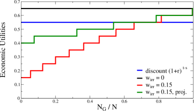
Figure 3: Pictorial representation of the economic utility in Equation (3) as a function of $n_{G}(t):=\frac{N_{G}(X_{t})}{N}$ for a fixed $t$ for different discount factors $g^{i}(t,s,n_{G}(t))$ as defined in Equation (5).

Before passing on the data description and the numerical experiments, we point out that we also write a macroscopic version of the two models introduced so far. We use this macroscopic version in some numerical experiments mainly for computational reasons. For ease of reading, we will confine its derivation in Appendix B, although it has an interest on its own.

3 Numerical experiments

In this section, we first described the data we will use in our analysis (Subsection 3.1), then we will present the model’s calibration (Subsection 3.2) and present the simulation results (Subsection 3.3).

3.1 Data description

In this subsection, we briefly describe the data used to fit the model; more details will be given in the next subsection.
As we are interested in the fraction of householder adopters of PV systems, in our numerical simulations, we focus on the number of installed PV systems between 2006 and 2020 (from GSE report [18]). In particular, the “Domestic” time series requires the following specification. In 2010-2020 we have explicit values of the “Domestic” data; the total national data is divided into the four categories described in the Introduction. In 2009 there was a different subdivision in categories from which we deduce that “Domestic” is approximately given by a certain percentage of the total; we have used this datum in the plots. Concerning 2006-2008 we do not even have the percentage. Specifically, we are considering the total number of PV systems installed, as PV systems are between 1 and 20 kW (the range of choice for householder adopters). The total number of PV systems is then normalized with the number of inhabited residential buildings, from ISTAT reports, 2011 (Data Source :  https://dati-censimentopopolazione.istat.it/).

3.2 Model’s calibration and inputs

Our models depend upon some parameters that must be calibrated to real data. The model’s calibration is inspired by what is usually done in the agent-based modeling literature (see, e.g., [13]) and named the indirect calibration approach. Several model runs are simulated, and the model’s results are compared with empirical data. The model parametrization that produces the best results is then chosen.
In more detail, the resulting values for the weights $w_{\text{ec}}$, $w_{\text{soc}}$ and $w_{\text{irr}}$ determine the average of a triangular distribution with support over $[0,1]$; notice that one of the most common distributions adopted in this type of literature is the triangular one. In principle, we can also consider time-varying weights and draw a different realization of the weights at each time step. However, since we will consider a “sufficiently” large number of agents in our numerical experiments, random weights $w_{soc},w_{ec}$ will be replaced by their average (cfr. also Appendix B). The same simplification cannot be applied for the weight $w_{irr}$ because it appears hidden in a non-linear function.

Alternatively, an interesting methodology is the one proposed in [36] for the diffusion of PV systems in the Netherlands. They identify four factors ((a) Advertising; (b) Neighborhood; (c) household income; (d) payback period of a PV system) and related to some aspects ((1) The contribution to a better natural environment; (2) The grant on offer; (3) The central organization of the request for a grant; (4) Independence from electricity supplier; (5) Discussion with other owners convinced me to adopt; (6) The buying of PV systems by neighbors/acquaintances; (7) The technical support offered by the municipality. To the latter, they assigned a score between 1 and 5 as in [35]. Then, the resulting triangular distribution’s support is $[1,5]$, and the mean is obtained from the average of the score of the pair factors-aspects. Although very interesting, we will leave this type of approach for further research.
We have decided to calibrate the model w.r.t the total number of PV systems that have been installed and not with respect the installed PV power. This choice is conductive to the interpretation of our models as models for describing the “Domestic” data’s PVs diffusion. We claim that the installed PV power is more suitable for the description of the “Agriculture”, “Industry” and “Service” data. Besides, we will consider PV systems between 1 and 20 kW, which is the usual range of choice for householder adopters. Also, we need to choose those Italian regions in which the percentage of “Domestic” installation is “sufficiently” large. This constraint justifies the choice of Liguria, Friuli Venezia Giulia, and Veneto for our analysis; the average percentage of “Domestic” installation with respect to the total power (Avg. $\%$) in such regions over 2010-2020 is reported in Table 1.

Region	Avg. $\%$ 2010-2020 PVs “Domestic”
Liguria	$23,48$
F. V. Giulia	$23,29$
Veneto	$19,05$

Table 1: Avg. $\%$ of “Domestic” PVs installation with respect the power over the period 2010-2020. Data Source :  GSE (https://www.gse.it/dati-e-scenari/statistiche).

Region	Ratio
Liguria	$0,61$
F. V. Giulia	$0,88$
Veneto	$3,80$

Table 2: Ratio between the number of inhabited buildings and the number or families. Data Source :  https://dati-censimentopopolazione.istat.it/.

Another variable choice is $N$, i.e., the number of agents in the system whose calibration is not straightforward. Indeed, the agents in our model are not single individuals but representative individuals of small communities, either a family or a condominium. For this reason, we will consider $N$ as the number of inhabited buildings. In order to understand if this datum is representative or not, we compute the ratio between the number of inhabited buildings and the number of families (Data Source :  https://dati-censimentopopolazione.istat.it/). Intuitively, this ratio indicates the reliability of the number of inhabited buildings as a representative datum for the number of individuals that decide to adopt PVs. Table 2 reports this ratio. An observation is in order. Veneto has a ratio greater than one. The reason can be the desertification of the center of Venice. In particular, if Ratio is less than one, the number of inhabited buildings is less than the number of families; in this case, we fix $N$ as the number of inhabited buildings. Instead, if the Ratio is greater than one, the number of inhabited buildings is greater than the number of families; in this case, for $N$, we will take a percentage of the number of inhabited buildings. In detail, as the total number of inhabited buildings represents an overestimate of our normalization factor $N$, we chose to consider the total number of PVs and not the precise percentage of residential PVs; this is a viable approach, as the number of residential PVs represents the more significant share. For folklore, one can think of this percentage as composed by the Italian SinusMilieus${}^{\tiny{\text{\textregistered}}}$ categories mentioned in [34], which we report in Appendix C for the sake of clarity.
At this point, we describe our model inputs. First, we need to compute the cash-flows in Equation (6). We start from the term $I_{\text{econ}}(t)$ in Equation (9); see Appendix A. The authors in [31] indicate the numerical values for the latter quantity. The index “Plant Cost compared to Modules Cost” (for the crystalline silicon) can be considered equal to a value between 1.5 and 1.9, the plant size is 3 kW. The previous computation gives a result comparable with the ”Turnkey PV system” (residential) average prices obtained from the National Survey Report of PV Power Applications in Italy. The evolution of the price per installed W of a PV system over the period 2007-2020 is displayed in Figure 4. Second, we need to recover the value for $E_{\text{PV}}(s)=E_{\text{Sun}}\cdot P_{\text{MPP}}\cdot(1-\xi_{\text{Abrasion}})^{s-t-1}$. Admittedly, we were not able to find in [34] and references therein a value for the coefficient of abrasion $\xi_{\text{Abrasion}}$. Therefore, we propose to use the following procedure. We define the value $E_{\text{PV}}(t)$ as the average of the amount of electricity generated by a household PV system located in Milano, Pisa, and Palermo, respectively (Data Source :  https://re.jrc.ec.europa.eu/pvg_tools/en/#api_5.1):

$$E_{\text{PV}}(t)=3\cdot\frac{(1310.32+1397.34+1523.02)}{3}\quad\textrm{kWh},$$

where the 3 in front of the equation indicates that we are considering PV system with a size of 3 kW. Then we assume that $E_{\text{PV}}(t)$ decreases of $3\%$ every year. With this datum we can then compute $R_{\text{Save}}(s,\text{CE5})$ by choosing $\chi_{DC}=0.85$, $p_{\text{elec,buy}}=0.18475$ Euro/kWh, $p_{\text{elec,sell}}=0.06101$ Euro/kWh, $\tau_{\text{elec,buy}}=0.04302$, $\tau_{\text{elec,sell}}=0.03211$. As we are not interested in an exact computation, we take the electricity prices as constant in the simulation. However, we checked that our model can still fit the data, with slightly different parameter values, if we consider electricity yearly medium prices. As regards as, instead, $R_{\text{Gov}}(s,\text{CE})$ it depends on the year at which the simulation start because of the difference in the values of the FiT (see Section 1.3). At this point, we need to specify the negative cash flows. As regards $R_{\text{Adm}}(s,\text{CE})$, we follow [34] and we set it equal to $3\frac{\text{Euro}}{\text{kW}\cdot\text{year}}$ for all the CE. As regards $R_{\text{Main}}$, we set its by choosing $\alpha_{\text{upfront}}=0.010$ and $\alpha_{\text{Main}}=0.013$. Finally, $R_{\text{time}}(s)$ is set to the standard value of $200$ Euro.

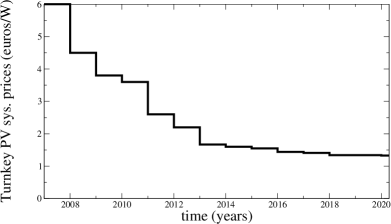
Figure 4: Turnkey PV system price per installed W of a PV system over 2007-2020, residential buildings. Data Source :  National Survey Report of PV Power Applications in Italy.

3.3 Simulations results

We simulate both the agent-based system and its mean field limit equations (see Appendix B). In the former case, we update the configurations on a monthly basis and we compute the sample mean and its standard deviation averaging on a total of 10000 samples. In the latter case, our time-step is taken to be much finer. In both cases, $R$ is taken to be constant for the entire year. As agents can be in different states, we have to specify the number of agents in each state at time zero. While the number of “Greens” is already fixed by the number of adopters in the year 2007, for the two categories of “Informed” and “Planners,” we have no means even to estimate a precise number. From our sensitivity analysis, we are, however, able to conclude that, given an initial number of agents in state $I$ or in state $P$, it is possible to find a corresponding number of agents in state $P$ or $I$ for which our model performs well, meaning that those parameters are highly correlated. We also deduce that there is not just one value of initial conditions for which the fit works well. However, it seems that the initial conditions for the number of “Informed” and “Planners” must be bigger than the initial conditions of “Green”. In particular, at the start of the simulation, we take as a plausible value for the number of “Planners” a multiple of the initial number of “Greens,” $k_{P}N_{G}$, with $k_{P}=10$. From our calibration, we then fix the number of agents in the state $I$ at time zero as $k_{I}N_{P}$, with $k_{I}=8$. We then keep those parameters constant in all our simulations, while determining different values for the parameters $w_{soc}$ and $w_{ec}$ for Italy and different regions from a least square minimization procedure. The optimal values for the weights are reported in Table 3; the value for $w_{\text{irr}}$ is maintained fixed to the value $w_{\text{irr}}=0.15$. We also report the calibrated weights in Figure 5 for a nicer representation.

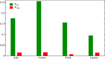
Figure 5: Influence of the weights $w_{ec}$ and $w_{soc}$ in the baseline scenario.

	$w_{ec}$	$w_{soc}$	$w_{irr}$	$k_{P}$	$k_{I}$	$T$
Italy	$0.17$	$0.01$	$0.15$	$10$	$8$	$3$
Veneto	$0.25$	$0.011$	$0.15$	$10$	$8$	$3$
Friuli	$0.15$	$0.0035$	$0.15$	$10$	$8$	$3$
Liguria	$0.09$	$0.01$	$0.15$	$10$	$8$	$3$

Table 3: Optimal value for the fitted weights.

Figures 6 shows the results of the calibration of the total number of adopters over the number of buildings in the chosen regions, both for the mean field model and for the particle system. In this latter case, we display the sample mean and its standard deviation. In particular, the different figures illustrate the actual PV market data and a simulation of the second model, which displays a very good fit to the actual number of adopters. Before commenting the results, the following observation regarding Figure 6 is in order. There are three distinct phases. At the initial formation phase, high costs (see Figure 4) and uncertainty result in a slow and erratic growth. This formative phase ends with a “take-off” which kicks the growth phase, in which growth accelerates due to positive feed-backs in economic profitability, technology learning and governmental support via the different phases of the CE. After achieving its maximum level, growth begins to slow mainly because of the eliminations of the incentives. Notice that we do not interpret, as in [8], this phase as a saturation phase.
In particular, the growth phase after the initial formation period is captured mainly by the variation in the economic utility: indeed in that period the $N_{G}$ curve mirrors the one of the payback period, for which we report a typical pattern over 2007–2020 in Figure 7. For comparison, we also report the payback period for an homo economicus agent who discounts the NPV via $(1+r)^{t-1}$, with $r$ being the interest rate; see Section 3.2. Notice that over 2013-2014 the payback period is decreasing although the governmental incentives are decreasing. This is due to the fall in price per installed W of a PV system (see Figure 4). Also, notice that with the introduction of the CE5 the payback period is less volatile. This observation suggests that the social influence between agents plays a crucial role in the the diffusion of PV system in the third phase. From the calibration we have that $w_{\text{ec}}$ is at least an order of magnitude greater than $w_{\text{soc}}$ for a fixed $w_{\text{irr}}$. This is in line with the results found in [34], where the influence of the communication network is negligible during the first two phases described above. Nonetheless, we point out that the weights coefficients should not be directly compared to each other because of the different formulations in their partial utilities, and their value should be interpreted as their relative importance in the adoption decision process. In particular, the situation $w_{\text{soc}}\approx w_{\text{ec}}$ would bring to an exponential growth over the entire period with a consequence misalignment of the payback period. In order to have a deeper understanding of the model, in the next subsection we perform a sensitivity analysis on the weights, and on the initial conditions $k_{I}$ and $k_{P}$. In particular, there may be other value combinations that could help achieve similar (or even) better calibration result since we do not study the convexity properties of the likelihood.

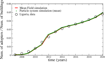
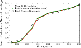
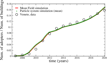
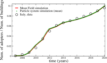
Figure 6: Calibration of the installed PV capacity, 2007–2020 for Liguria, Friuli Venezia Giulia, Veneto, and Italy. Source :  Own illustration, based on calibration results.

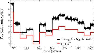
Figure 7: Example of a payback period of a PV system over 2007-2020, with the discount of the so called “homo economicus” and our discount where for each time $t$ $w_{irr}$ is a random variable with a triangular distribution with average $w_{irr}=0.15$

.

3.4 Sensitivity analysis

The results of the sensitivity analysis are summarized by Figures 8 and 9. The former displays the sensitivity concerning the weights (description in items (I), (II), and (III) below), and the latter for the initial conditions (description in item (IV) below). Sensitivity analysis is performed by holding constant the values of the calibrated parameters in the national data adaptation, see the first line of Table 3 and varying the parameter whose sensitivity is analyzed. In particular:

• The weight of the payback period $w_{\text{ec}}$ has, due to the linear formulation of its partial utility, a stronger impact on the diffusion process than that of the other weights. Indeed, our agents in passing from “Planner” to “Green” are homo economicus agents, which means that if $w_{\text{ec}}\approx 0$, then no transition occurs; see Section 2. We argue that this causality is not captured by models in which the transition occurs by evaluating a utility function expressed as the sum of weighted partial utilities accounting for different factors (e.g., the environmental benefit of investing in a PV system or the influence of communication with other agents). Indeed, in these models, the transition could happen even if it is not economically convenient.

• The weight $w_{\text{soc}}$ plays a very different role than the payback period weight. From Figure 8, Middle Panel, we observe that higher is the value of $w_{\text{soc}}$ and closer is our model to a logistic one. On the other hand, if $w_{\text{soc}}\approx 0$, then there is no transition; see the green line in the corresponding figure. More precisely, the transition $I\rightarrow PL\rightarrow G$ happens at a much faster rate than the transition $C\rightarrow I$, and, in practice, the Markovian model comes down to a model with states $\{C,PL,G\}$. Because the transition $C\rightarrow PL$ is not more allowed, no further transition is observed. Said differently, the state $I$ is not renovated rapidly enough.

• The parameter $w_{\text{irr}}$, kept constant at the value of 0.15 during the calibration procedure, influences, by construction, only the economic utility. In particular, when $w_{\textit{irr}}$ is a third of the calibrated value, our agents are neither homo economicus nor bounded rational (see the discussion at the end of Section 2, where the same effect is obtained by setting $N_{G}(X_{t})=N$), and they perceive a higher economic utility, thus obtaining a similar effect to an increase of $w_{\text{ec}}$; see item (I). On the other hand, an increase of $w_{\text{irr}}$ by 33$\%$ reflects that our agents may end up trapped in a procrastination loop due to the inter-temporal structure of the green choice. Therefore, the cumulative (normalized) number of adopters is still growing but slowing down.

• Finally, if the number of initial “Informed” or “Planner” agents increases, then a positive feedback loop is triggered and, as a consequence, also the number of “Green” increases, although at a different rate. More specifically, in our formulation, we assume that as the number of “Green” starts to increase, our agents are subject to an increasingly stronger incentive to invest in a PV system because of the presence of the term $\frac{N_{G}(X_{t})}{N}$ in both the economic utility and its projected version; see Figure 3. Notice, however, that if the fraction of agents who have adopted the PV system is not sufficiently large, roughly half of the total number, no transition from $I$ to $PL$ occurs.

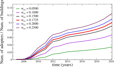
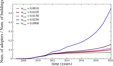
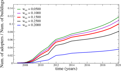
Figure 8: Sensitivity analysis on the weights. From top to bottom :  $w_{\text{ec}}$ and $w_{\text{irr}}$ fixed; $w_{\text{soc}}$ and $w_{\text{irr}}$ fixed; $w_{\text{ec}}$ and $w_{\text{soc}}$ fixed.

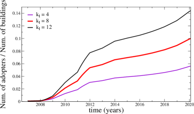
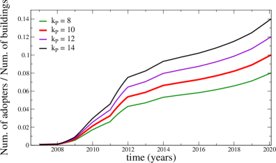
Figure 9: Sensitivity analysis on the initial number of agents in each state. From top to bottom :  $k_{P}$ fixed; $k_{I}$ fixed.

Notice that the sensitivity with respect to parameter $T$ has not been discussed, because the model does not show a relevant sensitivity with respect to this parameter. After that the model has been calibrated, it can be used to predict the future Italian PV market under various scenarios: this is the subject of the next section.

4 Scenario analysis

We test five different simulation scenarios to consider the sensitivity and validity of the proposed model. The first is a Baseline scenario where we use the set of parameters resulting from the calibration (see Section 3). Then, we consider a scenario with different PV investment costs (Scenario II), a policy-driven scenario with governmental PV support (Scenario III), a scenario in which a nudging strategy is implemented (Scenario IV), and a scenario in which social interaction is strengthened (Scenario V). All the Scenarios are built on the parametrization obtained from the calibration in Section 3. In addition, notice that the Scenarios are very different: Scenarios II–III are based on economic measures, whereas Scenarios IV–V is based on psychological or social dynamics.
Before discussing the results, an observation is in order. A reader could notice that we have not considered incentive schemes starting in 2023 aiming to provide incentives for the installation of PVs. The main reason is that in 2023 the Italian economy is still on the path to recovery from the COVID-19 pandemic and is affected by the armed conflict in Ukraine. Our model does not explicitly consider the irruptions of extreme events that disrupt the energy market. For this reason, we calibrated the model until 2020 in Section 3. Likewise, the different Scenarios must be contextualized to a standard economic environment.
For the reader’s convenience, we grouped the figures related to the scenario analysis at the end of the present section, in Subsection 4.6, in the order they will be cited. In addition, we will report the scenario analyses’ results for the Italian photovoltaic market; the results for the single regions are available from the authors upon request. For computational costs, all scenarios were realized by simulating the mean-field approximation.

4.1 Baseline scenario

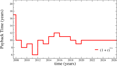
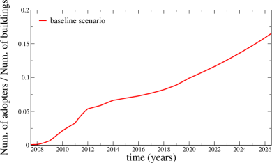
Figure 10: Italy, Baseline scenario. Top Panel: payback period of a PV system; Bottom Panel: number of installed PV system. Source :  Own illustration.

The Baseline scenario considers no further development of the Italian PV market throughout the simulation period ex-post the calibration (i.e., 2020-2026) and serves as a comparison with the other Scenario. In accordance, the payback period remains constant and equals its 2020 value; see Figure 10, Top Panel. Understanding the Baseline scenario can help us understand the decision-making process of the type of agents described in our model. The number of adopters will increase by $50\%$ from 2020 to 2025. As explained in Section 3, the influence of the network, social utility, and communication, in general, is significant in what we have denominated the “third phase”, in which the growth begins to slow mainly because of the elimination of the incentives. Therefore, in the Baseline scenario, the observed exponential growth in the third phase is primarily due to the communication network; see Figure 10, Bottom Panel.

4.2 Scenario I

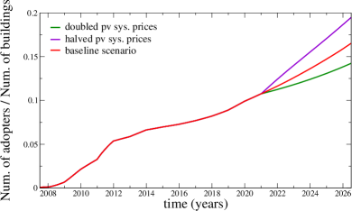
Figure 11: Italy, scenario I. Top Panel: payback period of a PV system; Bottom Panel: number of installed PV system. Source :  Own illustration

The first Scenario simulates two alternative PV system price developments. The two alternatives are based on an optimistic and a pessimistic outlook regarding future PV market development from the consumers’ perspective. The “high” PV system price alternative is obtained by increasing the PV system prices by $50\%$. The “low” one is obtained by decreasing the PV system prices by $50\%$. Again, as our model lacks realism over 2020-2023, we will not compare numerical simulations with actual data. Figure 11 collects the results. There is a clear difference relative to the Baseline scenario. A reduction in the investment costs leads to an increase in the total number of adopters of $17.34\%$ w.r.t the reference case at the end of the simulation period. In contrast, an increase in the investment cost slows the deployment process by $12.98\%$ w.r.t. the Baseline scenario. This result is not surprising since it has been shown that the economic profitability of the investment is the most influential criterion in the adoption decision. It is actually the criteria that enable the transition from “Planner” to “Green .” As a result, an increase (resp. a decrease) in the investment costs leads to a decrease (resp. an increase) in the payback period, in this case of two years; see Figure 11, Top Panel. Another parameter that most influence the investment’s economic profitability is the governmental support scheme, which characterizes Scenario II in the following subsection.

Remark 4.1.

We observe that introducing a carbon tax will produce an effect similar to that induced by the increase in initial investment. The introduction of a carbon tax would imply an increase in both prices $p_{purchase}$, $p_{sell}$, and thus $R_{save}$. This fact would make installing photovoltaics even more profitable and increase the number of adopters.

4.3 Scenario II

In this Scenario, a governmental incentive scheme is implemented. Again, the Baseline scenario is used as a reference for comparison. Changes to the support scheme occur from 2020 on-wards and produce the same effect on the payback period as halving prices; see Figure 12. More precisely, we maintain the same 2020 tax deductions, and we add a bonus equal to $E_{\text{PV}}\times 0.315$, where the quantity $E_{\text{PV}}$ is defined in Appendix A. The numerical result shows a difference with the Baseline scenario again. Compared to the latter, we observe an increase of $14.22\%$ in the number of PV installations at the end of the simulation period. One observation is in order. Although Scenario I and Scenario II produce the same change in the payback period, the former leads to a slighter higher number of adopters than Scenario II; see Figure 12, Bottom Panel. The hyperbolic discounting explains this discrepancy; see Figure 12, Middle Panel. The hyperbolic discounting of future utility can be seen as a temporary weakening of individual rationality induced by the approaching possibility of gains in the present. Hyperbolic discounting differs from exponential discounting of future utility, reflecting rational motives, such as considering the opportunity cost of capital ([2, 3, 6]). When looking at future choices, most people apply an exponential discount rate, which remains constant over time. For example, subject A might prefer to cash in USD 1,000 in 2030 rather than wait and cash in USD 1,100 in 2035, but A might agree to postpone the cash-in if he/she got USD 1,200 in 2035. In other words, the opportunity cost of tying up a capital of USD 1,000 is for A between USD 100 and 200. A applies a discount rate to the gain only for the time position the gain occupies. Economic theory postulates that if A prefers USD 1,200 in 2030 to USD 1,000 in 2035, then he/she must also prefer USD 1,200 in 2045 to USD 1,000 in 2040. And for most people, this is indeed the case. However, things change when the choices are not about future investments for even more future earnings but about present investments for future earnings. When the possibility to cash in the present approaches, the individual tends to apply a higher discount rate of future utility than he/she would apply for future investment choices with the same time distance to earnings. For example, A might be induced to prefer 1,000 euros today rather than 1,200 in 5 years, even though when faced with a choice between future investments for future earnings, he/she finds it rational to wait five years for a 20$\%$ gain on USD 1,000. The reasons for this temporary preference for smaller gains in the present are to be found in simple and irrational temporal myopia ([3]).

4.4 Scenario III

The third scenario involves implementing a policy to nudge people to transition to solar PV installation by acting on their psyche; we will refer to this policy as nudging. As said in Subsection 1.2, installing PVs is an inter-temporal choice. The distance between the time of the investment and the time of future earnings is one of the triggers of the procrastination phenomenon; see Subsection 1.2. Therefore, in the present scenario, we induce a distance reduction between the time of investment and that of future earnings by proposing to the individuals who want to install the PVs to agree on the installation at a certain date and to start paying for it at a specific date in the future.
We implement the nudging policy in the following way. We assume that starting from the year 2020, agents pass from $PL$ to $G$ in a time interval $\Delta t\rightarrow 0$ according to the following probability:

$$\begin{split}&\text{Prob}(X_{t+\Delta t}^{i}=G|X_{t}^{i}=PL):=w_{\text{ec}}^{i}\cdot U^{nudg}_{\text{ec}}\left(w_{\text{irr}}^{i},\frac{N_{G}(X_{t})}{N}\right).\end{split}$$

where the NPV in economic utility $U_{\text{ec}}^{nudg}$ is renewed by shifting the initial cost of the investment into the future time $t+T^{*}$, i.e., the NPV becomes:

$$\text{NPV}(t,n_{G}(t),\tau)=-\frac{I_{\text{econ}}(t)}{1+g^{i}(t,t+T^{*},n_{G}(t))}+\sum_{s=t+1}^{\tau}\frac{R(t-s)}{1+g^{i}(t,s,n_{G}(t)))}.$$

The transition from the state $I$ to the state $PL$ is modified accordingly, through the evaluation of

$$\text{NPV}(t,t+T,n_{G}(t),\tau)=-\frac{I_{\text{econ}}(t+T)}{1+g^{i}(t,t+T+T^{*},n_{G}(t))}+\sum_{s=t+T}^{\tau}\frac{R(s-(t+T-1))}{1+g^{i}(t,s,n_{G}(t))}.$$

Figure 13 displays the results when a nudging policy with $T^{*}=1.5$ years is implemented. The results indicate clear differences relative to the Baseline scenario. Nudging leads to an increment of $24.33\%$ in the total number of adopter w.r.t. the Baseline scenario at the end of the simulation period. Interestingly, while nudging does not affect the payback period of a homo economicus agent (Figure 13, Top Panel), it has an effect on agents’ payback period that is characterized by bounded rationality because of the presence of the hyperbolic discount (Figure 13, Middle Panel). In particular, by postponing the start of the investment, we mitigate the irrational behavior of the agent linked to procrastination.

4.5 Scenario IV

In this last scenario, we propose a strengthening of the agent’s communication network. One may find this proposal controversial because, as said, from the calibration, we have that $w_{\text{soc}}$ is at least an order of magnitude smaller than $w_{\text{ec}}$ for a fixed value of $w_{\text{irr}}$. However, we believe that it sheds some more light on the role of the weight $w_{\text{soc}}$ in the PV adoption dynamics. Figure 14 the results if we consider a value of $w_{\text{soc}}$ ten times greater than the calibrated value $w_{soc}=0.01$. We observe an increase of $97\%$ in the number of PV by the end of 2026. Moreover, what makes this scenario different from those previously proposed is the type of growth. Indeed, in this case, the growth is exponential, whereas in previous cases the growth was linear. This latter fact can be explained by observing the role of $w_{\text{soc}}$ in the so-called mean-field approximation of the model; see Equations (18) and (16). In particular, the density of the “Green” $n_{G}$ increases with the density of “Informed” agents $n_{I}$, whose density increases, modulated by $w_{soc}$ with $n_{G}$ itself. This means that $n_{G}$ increases exponentially with a rate proportional to $w_{soc}$. In any case, we believe that the growth observed in this scenario may be slightly overestimated. This could be explained by modeling assumptions. As we have already pointed out several times, agents interact in a mean-field way and this might have triggered an overestimation of the effect of social interaction. A more realistic way to describe the interaction between individuals is to consider a network-like structure; we propose to explore this in some future work.

4.6 Scenario analysis’ Figures

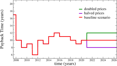
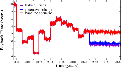
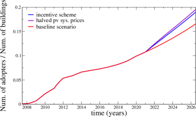
Figure 12: Italy, Scenario I and II. Top Panel: payback time of a PV system. Middle Panel: payback time discounted with the hyperbolic discount. Bottom Panel: number of installed PV system. Source :  Own illustration.

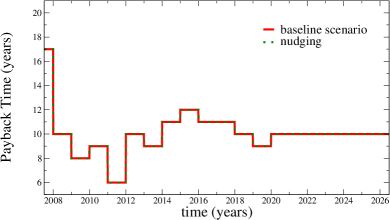
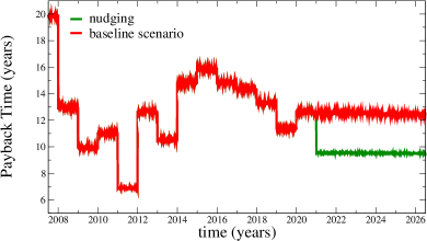
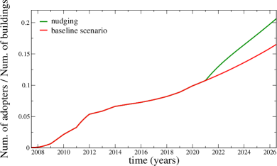
Figure 13: Italy, Scenario III. Top Panel: payback period of a PV system; Middle Panel: payback period of a PV system; Bottom Panel: number of installed PV systems. Source :  Own illustration.

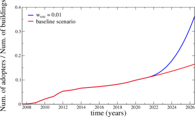
Figure 14: Italy, Scenario IV: number of installed PV systems. Source :  Own illustration.

5 Conclusions

The article presents two interesting ethical and political implications that lend themselves to further investigation, and which it is useful to emphasise in this concluding section.

First, the mathematical analysis of the data presented here shows that inter-temporal green choices are crucially influenced by cognitive biases such as hyperbolic discounting of individual future utility. This is both bad and good news for climate policies.

On the one hand, the policymaker must not only strive to ensure that the green choice is more economically rational than the status quo in a diachronic perspective, but must also address all those motivational barriers that prevent the individual agent from making the green choice, even where it is economically rational ([4]). In other words, it is not enough for the policymaker to deploy the classical tools of political economy, such as subsidies and taxes, in order to make the green choice more convenient and the status quo more unattractive; it is also necessary for the policymaker to provide agents with the means to overcome the impatience of the present, which many times pushes them to postpone choosing what is economically rational in the medium term ([1]).

On the other hand, the good news for policymakers is that they can rely on tools other than the classic economic ones, i.e. subsidies and taxes, which of course have the clear disadvantage of imposing costs on someone, usually the taxpayers ([27]). Nudging policies therefore play a central role in energy transition strategies, and as we know, the great advantage of these policies is that in most cases they come at little or no cost. The most obvious form of inter-temporal nudging is the separation in time between committing to a green choice and actually paying for it (see, e.g., [12, 30]. This is because if the hyperbolic discounting of the future utility of a green choice is associated with the approaching costs of the choice, then policymakers can take it upon themselves to allow the agent to choose at a point in time still far removed from the costs. In other words, policymakers can make the agent commit to the green choice before the cognitive biases of inter-temporal choice come into play. In order to do this, there is no need to give credit to the consumer, which would instead be a form of subsidy and thus at least have an opportunity cost. Policymakers can simply push companies to offer consumers prepurchase plans, in which both the payment of costs and the delivery of the product occur at a point in time after the commitment ([10]). How far the point in time of commitment should be from the final transaction is obviously something to be subject to further research. Here we merely observe that inter-temporal nudging is a powerful and greatly underestimated lever, at least so far, in the broad policy discourse on the energy transition.

Second, the paper shows how individual green choices do not only count for the GHG emissions that the agent abates through the green choice, but also for the effect that the individual green choice has on the chances that other individuals will also make similar choices, in turn abating other GHG emissions. One of the most discussed problems in individual climate ethics is individual causal inefficacy. The emissions that an individual abates by adopting a PV system have no or imperceptible impact on the mathematics of global warming: with or without the additional PV system, global temperature projections would be the same ([23] and [15]). The argument of individual causal inefficacy is often used to claim that the individual has no particular climate mitigation duties, as the real transition can only take place at the institutional level ([29]).

In contrast, the empirical results of the paper show a much more complex picture. Individual behaviour has social spillovers that go far beyond individual abatement potential. In fact, the individual who makes the green choice contributes more to climate mitigation by example than by the GHG emissions he/she abates. This may pave the way for a new and more complex theorisation of individual climate duties. On the other hand, individual climate duties consist in communicating to others that they have made the green choice, so as to contribute to the kind of contagion effect that makes the growth of installations go from linear to exponential. One could even make the paradox that communicating a green choice is more important than actually making it. This implies, in brief, that individual mitigation duties are broader than usually imagined. Communicating the green choice can in fact help to overcome various barriers on the part of those who have not yet made the choice, e.g. barriers of technical knowledge or economic viability, or it can even trigger social pressure mechanisms that are obviously reinforced as the number of agents who have made the green choice increases. Accordingly, the individual must convey in the most ramified way possible that he/she has embraced the green choice. The ways are the most diverse of course, from classic word of mouth, to internet and social network interaction, to simple exhibition.

Our hypothesis for future research is that the contagion effect found with PVs is even lower than the effect that could be found with other, more mobile and easily displayable green choices, such as those related to transport, diet, clothing, and so on. For instance, going beyond the specific topic of this article, it could be argued that the agent who buys an electric car contributes significantly to climate mitigation also, and perhaps above all, at the moment he/she drives the car, i.e. at the moment he/she conveys to others the message that he/she has chosen to drive an electric car.

ACKNOWLEDGMENT

The paper constitutes the second result of the interdisciplinary and inter-institutional research group working within the research project funded by the Italian Ministry of University and Research under the title: “Teorie e strumenti per la transizione ecologica: profili filosofici, matematici, etici e giuridici relativi alla sfida di sostenibilit‘a del carbon budget/Theories and tools for the ecological transition: philosophical, mathematical, ethical and juridical profiles related to the sustainability challenge of the carbon budget” (Prog. MURPRO3 2022-2024). It is a pleasure to thank GSE for providing us the data used in this work and, in particular, we thank Dr. Paolo Liberatore for his helpful clarifications. We thank Ing. Alberto Romagnoli for his insight and explanations on the net metering program. We gratefully acknowledge computational resources of the Center for High Performance Computing (CHPC) at SNS.

Appendix A Computation of the economic cost and of the cash flows

In this section, we describe the computation of the investment cost and the cash flows. This computation is based on [34], except for the computation of the investment costs $I_{\text{econ}}$. Indeed, in [34], the authors compute the investment costs by using a very precise formula involving the maximum peak power of the PV system, the available rooftop area for PV modules, the efficiency of the solar cells, the PV system efficiency, and the irradiation at standard conditions. Because in the present work we are trying to explain the general public’s behavior on the GET, we have judged the previous procedure too refined, and follow the ones in [26], where they provide a formula that enables the calculation of the cost of a given PV plant, on condition that the per-unit power module cost and the plant size are known. More precisely:

$$\begin{split}I_{\text{econ}}(t)=&\text{Modules Cost}[\text{Euro/Wp}]\\ &\times\text{Plant Size}[\text{Wp}]\times\text{Index ``Plant Cost compared to Modules Cost"}.\end{split}$$ (9)

The numerical values for the previous quantities are provided in the cited reference.
We now turn to the computation of the cash flow, and we start from the $R_{\text{Save}}(s,\text{CE})$. [34] provide an explicit expression for $R_{\text{Save}}(s,\text{CE})$ in the case of the CE 5:

$$\begin{split}R_{\text{Save}}(s,\text{CE}5)&=E_{\text{PV}}(s)\cdot\left[\chi_{\text{DC}}\cdot p_{\text{elec},\text{buy}}\cdot(1+\tau_{\text{elec},\text{buy}})^{s-t-1}\right.\\ &\left.+(1-\chi_{\text{DC}})\cdot p_{\text{elec},\text{sell}}\cdot(1+\tau_{\text{elec},\text{sell}})^{s-t-1}\right],\quad t\leq s\leq\tau.\\ \end{split}$$

where $E_{\text{PV}}(s)$ is the produced amount of electricity, $\chi_{\text{DC}}$ the share of direct electricity consumption and $p_{\text{elec},\text{buy}}$ (resp. $p_{\text{elec},\text{sell}}$) is the price of electricity bought (sold). The amount of electricity $E_{\text{PV}}$ generated by the system is a function of the level of irradiation $(E_{\text{Sun}})$, of the installed nominal maximum peak power $(P_{\text{MPP}})$, and of the predicted PV module abrasion $(\xi_{\text{Abrasion}})$:

$$E_{\text{PV}}(s)=E_{\text{Sun}}\cdot P_{\text{MPP}}\cdot(1-\xi_{\text{Abrasion}})^{s-t-1}.$$

Besides energy savings, an additional positive cash flow is generated by governmental support ($R_{\text{Gov}}(t,CE)$), which is based on the FiT (Feed in Tariff) given by the CE. The amount of the support is calculated as the sum of three components: a basic payment for the production of electricity ($\text{FiT}_{\text{Prod}}(CE)$), an incentive for direct PV electricity consumption ($\text{FiT}_{\text{DC}}(\text{CE})$), and, if applicable, additional bonuses ($\text{FiT}_{\text{Bon}}(\text{CE})$) that accrue in special circumstances. The cash flows associated with governmental support are then expressed as follows:

$$R_{\text{Gov}}(s,\text{CE})=E_{\text{PV}}(s)\cdot(\text{FiT}_{\text{Prod}}(\text{CE})+\text{FiT}_{\text{DC}}(\text{CE})+\text{FiT}_{\text{Bon}}(\text{CE}))$$ (10)

For instance in the CE 5 the governmental support is 200 Euro/kW and then decreases by either 15 $\%$ every six months, 5 $\%$ every six months and 25 $\%$ every six months. When there is no incompatibility with the benefits from the CEs, we add the additional benefits from the Net Metering scheme. After the end of the CEs, we consider the tax credit program, which consists of ten tax refunds, one for every year, of the size of a percentage of the initial investment, as done in [33]. We do not consider additional bonuses due to more invasive house renovations, as we suppose only a fraction of adopters could benefit from those bonuses.
As in [34], we assume that the adoption of a PV system also entails a series of negative cash flows. Administrative fees ($R_{\text{Adm}}(CE)$) have to be paid to the provider of the electricity grid and depend on the specific CE considered. For example, for CE 5 we have that:

$$R_{\text{Adm}}(\text{CE})=3\frac{\text{Euro}}{\text{kW}\cdot\text{year}}.$$

Maintenance costs ($R_{\text{Main}}(t)$) must also be considered. Upfront costs (e.g., the consultation of a PV expert/ adviser) are paid in the first year of the investment, while maintenance costs occur yearly. Both expenditures are estimated to be a fraction of the initial investment costs (as done in [34]):

$$R_{\text{Main}}(s)=\begin{cases}(\alpha_{\text{upfront}}+\alpha_{\text{Main}})\cdot I_{\text{econ}}\quad\text{if}\quad s=t\\ \,\alpha_{\text{Main}}\cdot I_{\text{econ}}\quad\quad\quad\quad\quad\quad\,\,\,\text{otherwise}.\end{cases}$$ (11)

Finally, the cash flow includes depreciation allowance payments of the PV system ($R_{\text{Deprec}}(s)$). The depreciation allowance amounts to a fixed outflow taking place at the end of every year for 20 years, at which point the remaining value of the fixed asset at the end of its useful lifetime is zero.

Appendix B A macroscopic view on the two Markovian models

We start from the first model. The idea is to find an evolution for quantities linked to the collective behaviour of the population. To this aim, let $X_{t}=(X_{t}^{1},\ldots,X_{t}^{N})\in\mathcal{S}$ be a generic configuration, $w_{\text{soc}}$, $w_{\text{irr}}$ and $w_{\text{ec}}$ be the weights defined in Section 2, $\mathcal{P}_{2}(\mathcal{S}\times\mathbb{R}^{3})$, $\mathcal{P}_{2}(\mathcal{S})$, and $\mathcal{P}_{2}(\mathbb{R})$ be the space of probability measures (on the corresponding spaces) that are square integrable. We suppose the weights are constant over time once the simulation starts, but they are also sampled from a distribution at time zero. In what follows, we will denote by capital letters the corresponding random variables. At this point, we can define the following quantities:

$$\begin{split}&\nu_{t}^{N}:=\frac{1}{N}\sum_{i=1}^{N}\delta_{\left(X^{i}_{t},w^{i}_{\text{soc}},w^{i}_{\text{ec}},w^{i}_{\text{irr}}\right)}\in\mathcal{P}_{2}\left(\mathcal{S}\times\mathbb{R}^{3}\right)\quad\,\,\mu^{N}_{t}:=\frac{1}{N}\sum_{i=1}^{N}\delta_{X^{i}_{t}}\in\mathcal{P}_{2}\left(\mathcal{S}\right)\\ &f^{N}_{\text{soc}}(dw_{\text{soc}}):=\frac{1}{N}\sum_{i=1}^{N}\delta_{w^{i}_{\text{soc}}}\in\mathcal{P}_{2}\left(\mathbb{R}\right)\quad\quad\quad f^{N}_{\text{ec}}(dw_{\text{ec}}):=\frac{1}{N}\sum_{i=1}^{N}\delta_{w^{i}_{\text{ec}}}\in\mathcal{P}_{2}\left(\mathbb{R}\right)\\ &\quad\quad\quad\quad\quad\quad\quad\quad f^{N}_{\text{irr}}(dw_{\text{irr}}):=\frac{1}{N}\sum_{i=1}^{N}\delta_{w^{i}_{\text{irr}}}\in\mathcal{P}_{2}\left(\mathbb{R}\right)\\ &n^{C,N}(X_{t}):=\frac{1}{N}\sum_{i=1}^{N}\mathds{1}_{\{X^{i}_{t}=C\}}\in(0,1)\quad\quad\quad\,\,n^{I,N}(X_{t}):=\frac{1}{N}\sum_{i=1}^{N}\mathds{1}_{\{X^{i}_{t}=I\}}\in(0,1)\\ &\quad\quad\quad\quad\quad\quad\quad\quad n^{G,N}(X_{t})=\frac{1}{N}\sum_{i=1}^{N}\mathds{1}_{\{X^{i}_{t}=G\}}\in(0,1).\end{split}$$ (12)

The goal is to find an expression for the evolution of $n^{C,N}(X_{t})$, $n^{I,N}(X_{t})$ and $n^{G,N}(X_{t})$. Toward this aim, we make the following assumption: We assume that the weights are independent from each other and independent from $X_{t}^{i}$ for each fixed $t$, i.e.:

$$\nu_{t}^{N}(dx,dw_{\text{soc}},dw_{\text{ec}},dw_{\text{irr}})=\mu^{N}(dx)\cdot f^{N}_{\text{soc}}(dw_{\text{soc}})\cdot f^{N}_{\text{ec}}(dw_{\text{ec}})\cdot f^{N}_{\text{irr}}(dw_{\text{irr}}).$$ (13)

Now, we consider an observable $F\,:\,\mathcal{S}\rightarrow\mathbb{R}$, $X:=(X^{1},\ldots,X^{N})\in\mathcal{S}$, and we assume that the process $X_{t}=(X_{t}^{1},\ldots,X_{t}^{N})$ is a continuous-time Markov chain (of cellular automaton type) with the following time-dependent infinitesimal generator:

$$\begin{split}\mathcal{L}_{t}F(X)&=\sum_{i=1}^{N}\mathds{1}_{\{X^{i}=C\}}\lambda_{N}^{C\to I}\left(w^{i}_{\text{soc}},n^{G,N}(X)\right)\left(F(X^{i,C\to I})-F(X)\right)\\ &+\sum_{i=1}^{N}\mathds{1}_{\{X^{i}=I\}}\lambda_{N}^{I\to G}\left(w^{i}_{\text{ec}},w^{i}_{\text{irr}},n^{G,N}(X)\right)\left(F(X^{i,I\to G})-F(X)\right)\\ \end{split}$$ (14)

At this point, we make the following

Remark B.1.

Notice that in our previous work [14] there were only two states $\{D,G\}$, where $D$ meant Deliberating and $G$ meant Green, and the rate of transition from $D$ to $G$ was a generic function $\lambda_{N}(X,t)=a(t)\cdot\frac{N_{G}(X)}{N}$. Indeed, it was sufficient only to fit the data with success.

At this point, we need to compute the following time-dependent infinitesimal generators:

$$\begin{split}\mathcal{L}_{t}n^{C,N}(X)&=\sum_{i=1}^{N}\mathds{1}_{\{X^{i}=C\}}\lambda_{N}^{C\to I}\left(w^{i}_{\text{soc}},n^{G,N}(X)\right)\left(n^{C,N}(X^{i,C\to I})-n^{C,N}(X)\right)\\ &+\sum_{i=1}^{N}\mathds{1}_{\{X^{i}=I\}}\lambda_{N}^{I\to G}\left(w^{i}_{\text{ec}},w^{i}_{\text{irr}},n^{G,N}(X)\right)\left(n^{C,N}(X^{i,I\to G})-n^{C,N}(X)\right)\\ &=-\frac{1}{N}\sum_{i=1}^{N}\mathds{1}_{\{X^{i}=C\}}\lambda_{N}^{C\to I}\left(w^{i}_{\text{soc}},n^{G,N}(X)\right)\\ &=-\int_{\mathbb{R}}w_{\text{soc}}\cdot n^{G,N}(X)\cdot f_{\text{soc}}^{N}(dw_{\text{soc}})\cdot n^{N,C}(X)\\ &=-\mathbb{E}^{N}\left[W_{\text{soc}}\right]\cdot n^{N,C}(X)\cdot n^{N,G}(X),\end{split}$$ (15)

where in the penultimate equality we use the rewriting of the term in terms of the measure $\nu^{N}$ and the independence between the random variables. By using the same argument, we can prove that $\frac{1}{N}\sum_{i=1}^{N}\mathds{1}_{X_{t}^{i}=I}\lambda_{N}^{I\rightarrow G}(w_{\text{ec}}^{i},w_{\text{irr}}^{i},n^{G,N}(X))=\mathbb{E}^{N}[W_{\text{ec}}]\cdot\mathbb{E}^{N}[U(W_{\text{irr}},n^{N,G}(X))]\cdot n^{N,I}(X)$. Therefore, the time-dependent infinitesimal generators $\mathcal{L}_{t}n^{I,N}(X)$ and $\mathcal{L}_{t}n^{G,N}(X)$ are given by

$$\begin{split}\mathcal{L}_{t}n^{I,N}(X)&=\mathbb{E}^{N}\left[W_{\text{soc}}\right]\cdot n^{C,N}(X)\cdot n^{G,N}(X)\\ &-\mathbb{E}^{N}\left[W_{\text{ec}}\right]\cdot\mathbb{E}^{N}[U(W_{\text{irr}},n^{N,G}(X))]\cdot n^{I,N}(X).\\ \mathcal{L}_{t}n^{G,N}(X)&=\mathbb{E}^{N}\left[W_{\text{ec}}\right]\cdot\mathbb{E}^{N}[U(W_{\text{irr}},n^{G,N}(X))]\cdot n^{I,N}(X).\end{split}$$

Finally, by Itô-Dynkin Equation (see [24], Appendix A), we deduce that the following system hold:

$$\begin{cases}n^{C,N}(X_{t})=n^{C,N}(X_{0})-\int_{0}^{t}\mathbb{E}^{N}\left[W_{soc}\right]n^{N,C}(X_{s})n^{N,G}(X_{s})ds+M_{t}^{N,C}\\ n^{I,N}(X_{t})=n^{C,N}(X_{0})+\int_{0}^{t}\mathbb{E}^{N}\left[W_{soc}\right]n^{N,C}(X_{s})n^{N,G}(X_{s})ds+\\ \quad\quad\quad\quad\quad\quad\quad-\int_{0}^{t}\mathbb{E}^{N}\left[W_{ec}\right]\cdot\mathbb{E}^{N}\left[U(W_{irr},n^{N,G}(X_{s}))\right]n^{I,N}(X_{s})ds+M_{t}^{N,I}\\ n^{G,N}(X_{t})=n^{G,N}(X_{0})-\int_{0}^{t}\mathbb{E}^{N}\left[W_{ec}\right]\cdot\mathbb{E}^{N}\left[U(W_{irr},n^{N,G}(X_{s}))\right]n^{I,N}(X_{s})ds\\ \quad\quad\quad\quad\quad\quad\quad+M_{t}^{N,G},\\ \end{cases}$$

where $M_{t}^{N,C},M_{t}^{N,I},M_{t}^{N,G}$ are martingales, of which we know certain properties by the second Itô-Dynkin equation (see, again, [24], Appendix A). Taking the limit for $N\rightarrow\infty$, we get the final system of equations:

$$\begin{cases}\frac{d}{dt}n^{C}_{t}(X)=-\mathbb{E}\left[W_{soc}\right]\cdot n^{C}_{t}(X)\cdot n^{G}_{t}(X)\\ \frac{d}{dt}n^{I}_{t}=\mathbb{E}\left[W_{soc}\right]\cdot n^{C}_{t}(X)\cdot n^{G}_{t}(X)-\mathbb{E}\left[W_{ec}\right]\cdot\mathbb{E}\left[U(W_{irr},n^{G})\right]\cdot n^{I}_{t}(X)\\ \frac{d}{dt}n^{G}_{t}=\mathbb{E}\left[W_{ec}\right]\cdot\mathbb{E}\left[U(W_{irr},n^{G})\right]\cdot n^{I}_{t}(X)\\ \end{cases}$$ (16)

As regards as the second model, because of the presence of the additional state $PL$, we need to define the following (additional) quantity: $n^{PL,N}(X_{t}):=\frac{1}{N}\sum_{i=1}^{N}1_{\{X_{t}^{i}=PL\}}$, for which we will determine its dynamics later on. In particular, we have to consider a new observable $F\,:\,\mathcal{S}\rightarrow\mathbb{R}$ and the new state-space $\mathcal{S}:=\{C,I,PL,G\}$. Again, assuming that the process $X_{t}=(X_{t}^{1},\ldots,X_{t}^{N})$ is a continuous-time Markov chain (of cellular automation type), in this case the time-dependent infinitesimal generator is given by:

$$\begin{split}\mathcal{L}_{t}F(X)&=\sum_{i=1}^{N}\mathds{1}_{\{X^{i}=C\}}\lambda_{N}^{C\to I}\left(w^{i}_{\text{soc}},n^{G,N}(X)\right)\left(F(X^{i,C\to I})-F(X)\right)\\ &+\sum_{i=1}^{N}\mathds{1}_{\{X^{i}=I\}}\lambda_{N}^{I\to G}\left(w^{i}_{\text{ec}},w^{i}_{\text{irr}},n^{G,N}(X)\right)\left(F(X^{i,I\to G})-F(X)\right)\\ &+\sum_{i=1}^{N}\mathds{1}_{\{X^{i}=PL\}}\lambda_{N}^{PL\to G}\left(w^{i}_{\text{ec}},w^{i}_{\text{irr}},n^{G,N}(X)\right)\left(F(X^{i,PL\to G})-F(X)\right).\\ \end{split}$$ (17)

In addition, the time-dependent infinitesimal generators $\mathcal{L}_{t}n^{C,N}$, $\mathcal{L}_{t}n^{I,N}$, $\mathcal{L}_{t}n^{PL,N}$ and $\mathcal{L}_{t}n^{G,N}$ are given by:

$$\begin{split}\mathcal{L}_{t}n^{C,N}(X)&=-\mathbb{E}\left[W_{\text{soc}}\right]\cdot n^{C,N}(X)\cdot n^{G,N}(X)\\ \mathcal{L}_{t}n^{I,N}(X)&=\mathbb{E}^{N}\left[W_{\text{soc}}\right]\cdot n^{C,N}(X)\cdot n^{G,N}(X)\\ &-\mathbb{E}^{N}\left[W_{\text{ec}}\right]\cdot\mathbb{E}^{N}[U(W_{\text{irr}},n^{N,G}(X))]\cdot n^{I,N}(X).\\ \mathcal{L}_{t}n^{PL,N}(X)&=\mathbb{E}^{N}\left[W_{\text{ec}}\right]\cdot\mathbb{E}^{N}[U(W_{\text{irr}},n^{G,N}(X))]\cdot n^{I,N}(X)\\ &-\mathbb{E}^{N}\left[W_{\text{ec}}\right]\cdot\mathbb{E}^{N}[U(W_{\text{irr}},n^{N,G}(X))]\cdot n^{PL,N}(X).\\ \mathcal{L}_{t}n^{G,N}(X)&=\mathbb{E}^{N}\left[W_{\text{ec}}\right]\cdot\mathbb{E}^{N}[U(W_{\text{irr}},n^{G,N}(X))]\cdot n^{I,N}(X).\end{split}$$

By arguing as above, we can obtain the following final system of ordinary differential equations:

$$\begin{cases}\frac{d}{dt}n^{C}(X)=-\mathbb{E}\left[W_{\text{soc}}\right]\cdot n^{C}_{t}(X)\cdot n^{G}_{t}(X)\\ \frac{d}{dt}n^{I}_{t}(X)=\mathbb{E}\left[W_{\text{soc}}\right]\cdot n^{C}_{t}(X)\cdot n^{G}_{t}(X)\\ \quad\quad\quad\quad\quad-\mathbb{E}\left[W_{\text{ec}}\right]\cdot\mathbb{E}\left[U^{\text{proj}}_{\text{ec}}\left(W_{\text{irr}},T,n^{G}_{t}(X)\right)\right]n^{I}_{t}(X)\\ \frac{d}{dt}n^{PL}_{t}(X)=\mathbb{E}\left[W_{\text{ec}}\right]\cdot\mathbb{E}\left[U^{\text{proj}}_{\text{ec}}\left(W_{\text{irr}},T,n^{G}_{t}\right)\right]\cdot n^{I}(X)\\ \quad\quad\quad\quad\quad-\mathbb{E}\left[W_{\text{ec}}\right]\mathbb{E}\left[U_{\text{ec}}\left(W_{\text{irr}},n^{G}_{t}(X)\right)\right]n^{PL}_{t}(X)\\ \frac{d}{dt}n^{G}_{t}(X)=\mathbb{E}\left[W_{\text{ec}}\right]\cdot\mathbb{E}\left[U_{\text{ec}}\left(W_{\text{irr}},n^{G}_{t}(X)\right)\right]\cdot n^{PL}_{t}(X).\\ \end{cases}$$ (18)

At this point, the following important remark on the weights is in order.

Remark B.2.

The dependence on the weights $w_{\text{ec}}^{i}$ and $w_{\text{soc}}^{i}$ is linear in the transition rates, whereas the dependence on $w_{\text{irr}}^{i}$ is non-linear. In addition, the distribution matters and it appears in the term $\mathbb{E}\left[U_{\text{ec}}\left(W_{\text{irr}},n^{G}_{t}(X)\right)\right]$.

Appendix C Description of the Italian Sinus-Milieus${}^{\tiny{\text{\textregistered}}}$ categories adopted in the present paper

The following Table 4 report the description of the Sinus-Milieus${}^{\tiny{\text{\textregistered}}}$ categories used in the present study. The source is Appendix A.1, Table 11, in [34].

Sinus-Milieus${}^{\tiny{\text{\textregistered}}}$	Borghesia Illuminata (enlightened middle class)
Characteristics	Highest lifestyle, society’s elite, econ. thinking
Type of household	Couples, sometimes with children
Age	Older than 45 years
Education	Highest education
Work	Businessmen, qualified employees and executives
Income	Highest income
Share of population	5.7 million inhabitants (10$\%$ of population)
Sinus-Milieus${}^{\tiny{\text{\textregistered}}}$	Progressisti Tolleranti (intellectuals)
Characteristics	Critical intellectuals, socially ambitious
Type of household	Couples, sometimes with children
Age	40–60 year
Education	High and highest education
Work	Freelance, executive employees
Income	Freelance, executive employees
Share of population	5.7 million inhabitants (10$\%$ of population)
Sinus-Milieus${}^{\tiny{\text{\textregistered}}}$	Edonisti Ribelli (experimentalists)
Characteristics	Modern and creative, open to new ideas
Type of household	Small families and singles
Age	Younger than 35 years
Education	Higher education
Work	Freelancer, executive employees
Income	Average income
Share of population	4.1million inhabitants (7$\%$ of population)

Table 4: Detailed description of the Italian Sinus-Milieus${}^{\tiny{\text{\textregistered}}}$ categories adopted in the present paper.

References

- [1] Ainslie, G., (2010). Procrastination, the basic impulse. In The Thief of Time: Philosophical Essays on Procrastination. Edited by c. Andreou and M. D. White, Oxford University Press. 11–27.
- [2] Ainslie, G., (2012). Pure hyperbolic discount curves predict “eyes open” self-control. Theory and Decision. 73(1):3-34.
- [3] Ang, N., (2012). Procrastination as Rational Weakness of Will. Journal of Value Inquiry. 46:403–416.
- [4] Andreou, C., (2007). Environmental Preservation and Second-Order Procrastination. Philosophy Public Affairs. 35:233-248.
- [5] Bass, F. M., (1969). A new product growth for model consumer durables. Management Science. 15(5):215–227.
- [6] Batini, N., Melina, G., Di Serio, M., Fragetta, M., (2021). Building back better: how big are green spending multipliers?. Technical Report.
- [7] Bisin, A., Hyndman, K., (2020). Present-bias, procrastination and deadlines in a field experiment. Games and Economic Behavior. 119:339–357.
- [8] Cherp, A., Vinichenko, V., Tosun, J., Gordon, J. A., Jewell, J., (2021). National growth dynamics of wind and solar power compared to the growth required for global climate targets. Nature Energy. 6(7):742–754.
- [9] Colasante, A., D’Adamo, I., Morone, P., (2021). Nudging for the increased adoption of solar energy? Evidence from a survey in Italy. Energy Research Social Science. 74:101978.
- [10] Corvino, F., (2021). Climate Change, Individual Preferences, and Procrastination. In Climate Justice and Feasibility: Normative Theorizing, Feasibility Constraints, and Climate Action. Edited by Sarah Kenehan and Corey Katz. 193–212.
- [11] Da Silva, H. B., Uturbey, W., Lopes, B.M., (2020). Market diffusion of household PV systems: Insights using the Bass model and solar water heaters market data. Energy for Sustainable Development. 55:210–220.
- [12] Elster, J., (2000). Ulysses Unbound: Studies in Rationality, Precommitment, and Constraints. Cambridge: Cambridge University Press.
- [13] Fagiolo, G., Moneta, A., Windrum, P., (2007). A critical guide to empirical validation of agent-based models in economics: Methodologies, procedures, and open problems. Computational Economics. 30:195–226.
- [14] Flandoli, F., Corvino, F., Leocata, M., Livieri, G., Morlacchi, S., Pirni, A., (2022). Multiscale modeling of Green Energy Transition: Structural properties and an example. Available at: arXiv:2212.01329v1.
- [15] Fragniére, A, (2016). Climate change and individual duties. WIREs Climate Change. 7:798-814.
- [16] Gifford, R., (2011). The dragons of inaction: psychological barriers that limit climate change mitigation and adaptation. American Psychologist. 66(4):290.
- [17] Graczyk, A. M., (2021). Households behaviour towards sustainable energy management in Poland — The homo energeticus concept as a new behaviour pattern in sustainable economics. Energies. 14(11):3142.
- [18] GSE, Gestore dei Servizi Energetici SpA (2007-2020).
- [19] IEA, (2019). World Energy Outlook, p. 2019.
- [20] IPCC, (2018). Global Warming of 1.5 ∘C. An IPCC Special Report on the impacts of global warming of 1.5 ∘C above pre-industrial levels and related global greenhouse gas emission pathways, in the context of strengthening the global response to the threat of climate change, sustainable development, and efforts to eradicate poverty.
- [21] Jackson, T., (2005). Live better by consuming less?: is there a “double dividend” in sustainable consumption?. Journal of Industrial Ecology. 9(1-2):19–36.
- [22] Karakaya, E., (2016). Finite Element Method for forecasting the diffusion of photovoltaic systems: Why and how?. Applied Energy. 163:464–475.
- [23] Kingston, E., Sinnott-Armstrong, W. (2018). What’s Wrong with Joyguzzling?. Ethical Theory and Moral Practice. 21:169–186.
- [24] Kipnis, C., Landim, C., (1998). Scaling limits of interacting particle systems, Volume 320. Springer Science Business Media.
- [25] Kotilainen, K., Valta, J., Mäkinen, S. J., Järventausta, P., (2017) Understanding consumers’ renewable energy behaviour beyond “homo economicus”: An exploratory survey in four European countries, 2017 14th International Conference on the European Energy Market (EEM). 1–6.
- [26] Krumm, A., Susser, D., Blechinger, P., (2022). Energy. 239:121706.
- [27] Lepenies, R. and Malecka, M., (2019). The ethics of behavioural public policy . In The Routledge Handbook of Ethics and Public Policy, Edited by Annabelle Lever and Andrei Poama. 513–524
- [28] Luthra, S., Sanjay, K., Ravinder, K., Md Fahim, A., SL, S., (2014). Adoption of smart grid technologies: An analysis of interactions among barriers. Renewable and Sustainable Energy Reviews, 333:554–565.
- [29] Maclean, D., (2019). Climate Complicity and Individual Accountability. The Monist. 102(1):1–21.
- [30] Maltais, A., (2015). Making our children pay for mitigation. In The Ethics of Climate Governance, Edited by A. Maltais C. McKinnon, pp. 91–110. Lanham, MD: Rowman Littlefield International.
- [31] Mazzanti, G., Romito Zaccagnini, D., (2012). Innovative Investigation about the payback time of photoltaic plants in Italy. IIETA, 69–76.
- [32] Orioli, A., Di Gangi A., (2015) . The recent change in the Italian policies for photovoltaics: Effects on the payback period and levelized cost of electricity of grid-connected photovoltaic systems installed in urban contexts. Energy 93:1989-2005.
- [33] Peralta, A. A., Balta-Ozkan, N., Longhurst, P., (2022). Spatio-temporal modelling of solar photovoltaic adoption: An integrated neural networks and agent-based modelling approach. Applied Energy, 305:117949.
- [34] Palmer, J., Sorda, G., Madlener, R., (2015). Modeling the diffusion of residential photovoltaic systems in Italy: An agent-based simulation. Technological Forecasting and Social Change, 99:106–131.
- [35] Jager, W., (2006). Stimulating the diffusion of photovoltaic systems: A behavioural perspective. Energy Policy., 34(14): 1935–1943.
- [36] Zhao, J., Mazhari, E., Celik, N., Son, Y.J. (2011). Hybrid agent-based simulation for policy evaluation of solar power generation systems. Simulation Modelling Practice and Theory. 19(10):2189–2205.
- [37] Galam, S., Moscovici, S.. (1991). Towards a theory of collective phenomena: Consensus and attitude changes in groups. European Journal of Social Psychology. 21.1 : 49-74.
- [38] Holley, R.A., Liggett, T.M.. (1975). Ergodic theorems for weakly interacting infinite systems and the voter model. The annals of probability. 643-663.
- [39] Lewenstein, M., Nowak, A., Latané, B.. (1992). EStatistical mechanics of social impact. Physical Review A. 45.2: 763.
- [40] Sîrbu, A., Loreto, V., Servedio, V. D., Tria, F.. (2017). Opinion dynamics: models, extensions and external effects. . Participatory sensing, opinions and collective awareness. 363-401.