A Data-Driven Approach for Bayesian Uncertainty Quantification in Imaging

Abstract

Uncertainty quantification in image restoration is a prominent challenge, mainly due to the high dimensionality of the encountered problems. Recently, a Bayesian uncertainty quantification by optimization (BUQO) has been proposed to formulate hypothesis testing as a minimization problem. The objective is to determine whether a structure appearing in a maximum a posteriori estimate is true or is a reconstruction artifact due to the ill-posedness or ill-conditioness of the problem. In this context, the mathematical definition of having a “fake structure" is crucial, and highly depends on the type of structure of interest. This definition can be interpreted as an inpainting of a neighborhood of the structure, but only simple techniques have been proposed in the literature so far, due to the complexity of the problem. In this work, we propose a data-driven method using a simple convolutional neural network to perform the inpainting task, leading to a novel plug-and-play BUQO algorithm. Compared to previous works, the proposed approach has the advantage that it can be used for a wide class of structures, without needing to adapt the inpainting operator to the area of interest. In addition, we show through simulations on magnetic resonance imaging, that compared to the original BUQO’s hand-crafted inpainting procedure, the proposed approach provides greater qualitative output images. Python code will be made available for reproducibility upon acceptance of the article.

I Introduction

Imaging problems across many modes, disciplines and scales can be stated as inverse problems. Usually, one aims to find an estimate ${\mathb{x}}^{\dagger}\in{\mathbb{R}}^{N}$ of an original unknown image $\overline{{\mathb{x}}}\in{\mathbb{R}}^{N}$, from degraded measurements ${\mathb{y}}\in{\mathbb{C}}^{M}$, observed through a linear model of the form

$${\mathb{y}}={\boldsymbol{\Phi}}\overline{{\mathb{x}}}+{\mathb{w}}.$$ (1)

Here ${\boldsymbol{\Phi}}\colon{\mathbb{R}}^{N}\to{\mathbb{C}}^{M}$ is the measurement operator, which we assume to be known and linear, and ${\mathb{w}}\in{\mathbb{C}}^{M}$ is a realization of a independent identically distributed (iid) random variable. In general, this inverse problem is ill-posed and/or ill-conditioned, so the estimate ${\mathb{x}}^{\dagger}$ cannot be obtained with a direct model, and iterative approaches are required.

Following a Bayesian framework, the posterior distribution of the problem can be expressed as

$${\mathsf{P}}({\mathb{x}}\mid{\mathb{y}})\propto\exp\Big{(}-f_{\mathb{y}}({\boldsymbol{\Phi}}{\mathb{x}})-g({\mathb{x}})\Big{)}.$$

This formulation combines information from the likelihood and the prior, encoded by $f_{\mathb{y}}({\boldsymbol{\Phi}}\,\cdot)$ and $g$, respectively. The prior is used to incorporate a priori information known about the image of interest, to help to overcome ill-posedness and/or ill-conditionedness of the inverse problem. Classical choices include feasibility constraints (e.g., positivity for intensity images), or functions promoting either smoothness or sparsity (e.g., $\ell_{2}$ or $\ell_{1}$ norms) possibly in some transformed domain such as wavelet, Fourier or total variation (TV) (see e.g., [1, 2]). A classical inference approach is to find a maximum a posteriori (MAP) estimator, defined as

$${\mathb{x}}^{\dagger}=\underset{\begin{subarray}{c}{{\mathb{x}}\in{\mathbb{R}}^{N}}\end{subarray}}{\mathrm{Argmin}}\;\;f_{{\mathb{y}}}({\boldsymbol{\Phi}}{\mathb{x}})+g({\mathb{x}}).$$ (2)

Problem (2) can be solved efficiently using optimization algorithms. Since early 2000’s, proximal algorithms have been the state-of-the-art in imaging problems [3, 4, 5, 6, 7, 8, 9, 10, 11, 12]. They are scalable to high-dimensional problems, and versatile to handle sophisticated problems involving non-smooth functions and linear operators. During the last decade, these algorithms have been significantly improved by the adoption of deep learning. Specifically, to improve the reconstruction quality of proximal algorithms, the operator handling the prior term has been replaced by a neural network (NN), trained to perform a denoising task. The resulting algorithms belong to a library of so-called “plug-and-play” (PnP) methods and have proved to be very successful in image restoration [13, 14, 15, 16]. Recently a lot of attention has been paid to better understand the theoretical guarantees for PnP algorithms [15, 17, 18, 19, 20, 21, 22, 23].

Although proximal optimization algorithms are very efficient and widely used for finding MAP estimates, they provide a point estimate only, without any additional information. In the absence of the ground truth, these approaches do not quantify any of the inherent uncertainties in such estimates. Uncertainty quantification (UQ) provides rigorous additional information to accompany qualitative estimates, and the rich theory of Bayesian inference can provide such analyses. UQ can be of great benefit with respect to decision making, for example using medical magnetic resonance (MR) scans to plan a course of treatment, where it is very important to know whether or not specific structures in a MAP estimate can be trusted to a quantified measure of certainty.

Classically, sampling methods such as Markov chain Monte Carlo (MCMC) are used to generate estimators of the original unknown image by drawing random samples from the posterior distribution, and hence approximating the true distribution of interest [24, 25]. Such methods allow to perform UQ by confidence intervals and hypothesis testing. Unfortunately, traditional MCMC methods are not adapted to imaging problem, due to their high dimension. Recently, many authors have proposed to pair MCMC with optimization techniques to make them more scalable (see e.g., [26, 27, 28, 29, 30, 31]). Although these methods do offer more scalable approaches to draw each sample, they still draw huge numbers of samples to achieve a satisfactory approximation of the distribution of interest (due to the size $N$ of the image, i.e., the unknown parameters).

Recently, another hybrid technique has been proposed to perform scalable UQ for imaging, dubbed BUQO [31, 32, 33, 34, 35, 36]. This approach is different from the hybrid MCMC methods described above, in that it uses optimization algorithms to compute both the MAP estimate and the UQ. In a nutshell, it computes the MAP estimate, and then performs a hypothesis test only on questionable structures identified in the MAP estimate. The hypothesis test itself is defined as a minimization problem, and solved by leveraging the same scalable proximal algorithms as used to obtain the MAP estimate. Such an approach is then more scalable than traditional MCMC algorithms, in particular in a high dimensional setting where computing the MAP is much cheaper than estimating the posterior distribution. Nevertheless, the mathematical definition of having a “fake structure" in the MAP estimate is crucial, and highly dependent on the type of structure of interest. This definition can be interpreted as an inpainting task, but only simple hand-crafted techniques have been proposed in the literature so far, due to the complexity of the problem.

In this work, we propose a data-driven approach relying on a convolutional neural network (NN) for the inpainting task in BUQO. This allows for a simplified formulation of the original minimization problem proposed in [33], to perform the hypothesis test. In this formulation, the inpainting NN explicitly appears in a squared $\ell_{2}$ function, that will be handled exclusively through its gradient in a PnP algorithm based on a primal-dual forward-backward algorithm [7, 8, 37]. Although the proposed method aims to use the NN not as a denoiser, as done in standard PnP, the notion of “plugging in” the inpainting NN is very similar. Indeed, the objective is to replace a task that could be done by standard optimization tools, such as a gradient or proximity operator, by a NN specifically trained for the task. We highlight the performances of the proposed approach, dubbed PnP-BUQO, to perform UQ on a simulated MR imaging problem. In particular, we show that the proposed PnP-BUQO enables more realistic visual results compared to the original BUQO inpainting version.

The remainder of the article is organized as follows. Section II covers the relevant background material in Bayesian statistics. We formulate hypothesis tests corresponding to BUQO and PnP-BUQO in Section III, and introduce proximal splitting algorithms to evaluate them. Section IV discusses algorithms to evaluate the proposed hypothesis tests. In Section VI we detail simulations which demonstrate the PnP-BUQO method, using a NN, detailed in Section V, and we conclude in Section VII with a high-level evaluation of our method and proposals for further research.

II Bayesian background and BUQO principle

II-A Hypothesis test setting

As emphasized in the introduction, there is significant uncertainty when computing a MAP estimate ${\mathb{x}}^{\dagger}$ due to the inherent ill-posed or ill-conditioned nature of model (1). The MAP estimate itself is a point estimate only, and hence there is no quantification of uncertainty. The BUQO method proposed in [33] evaluates a Bayesian hypothesis test on the degree of support for specific image structures appearing in the MAP estimate ${\mathb{x}}^{\dagger}$ (e.g., lesions in medical imaging, or celestial sources in astronomical imaging). This test is defined by postulating two hypotheses:

$H_{0}$: Structure of interest ABSENT in the ground truth;

$H_{1}$: Structure of interest PRESENT in the ground truth.

To perform this hypothesis test without stochastic sampling, BUQO leverages the scalability of convex optimization methods to assert with confidence $\alpha\in]0,1[$ whether $H_{0}$ can be rejected in favor of $H_{1}$. Formally, $H_{0}$ is rejected with significance $\alpha$ if

$${\mathsf{P}}(H_{0}\mid{\mathb{y}})\leqslant\alpha,$$ (3)

in which case ${\mathsf{P}}(H_{1}\mid{\mathb{y}})>1-\alpha$.

II-B BUQO hypothesis testing

In [33], the authors associate the null hypothesis $H_{0}$ with the set of all possible images of $\mathbb{R}^{N}$ not containing the structure, denoted ${\mathcal{S}}\subset\mathbb{R}^{N}$. Then, we have ${\mathsf{P}}(H_{0}\mid{\mathb{y}})={\mathsf{P}}(\overline{{\mathb{x}}}\in{\mathcal{S}}\mid{\mathb{y}})$. Thereafter, they propose to evaluate condition (3) by comparing ${\mathcal{S}}$ with a conservative credible region $\widetilde{{\mathcal{C}}}_{\alpha}$, with confidence level $1-\alpha$, which is defined such that ${\mathsf{P}}(\overline{{\mathb{x}}}\in\widetilde{{\mathcal{C}}}_{\alpha}\mid{\mathb{y}})\geqslant 1-\alpha$. The advantage of using this conservative credible region over the true credible region, is that the set has an explicit formulation that does not require expensive integrals over $\mathbb{R}^{N}$ to be evaluated. Indeed, in [32] the author proposes to compute $\widetilde{{\mathcal{C}}}_{\alpha}$ as a by-product of MAP estimation. Specifically, given a MAP estimate ${\mathb{x}}^{\dagger}$ solving of (2), this set is defined as

$$\widetilde{{\mathcal{C}}}_{\alpha}=\big{\{}{{\mathb{x}}\in\mathbb{R}^{N}}\leavevmode\nobreak\ \big{|}\leavevmode\nobreak\ {f_{{\mathb{y}}}({\boldsymbol{\Phi}}{\mathb{x}})+g({\mathb{x}})\leqslant\widetilde{\eta}_{\alpha}}\big{\}},$$ (4)

where $f_{{\mathb{y}}}$ and $g$ are defined in (2), and $\widetilde{\eta}_{\alpha}=f_{{\mathb{y}}}({\boldsymbol{\Phi}}{\mathb{x}}^{\dagger})+g({\mathb{x}}^{\dagger})+N(\sqrt{16\log(3/\alpha)/N}+1)$.

The sets ${\mathcal{S}}$ and $\widetilde{{\mathcal{C}}}_{\alpha}$, satisfy the following result.

Theorem II.1.

[33, Thm 3.2] Suppose that $\alpha\in]4\exp(-N/3),1[$. If ${\mathcal{S}}\cap\widetilde{{\mathcal{C}}}_{\alpha}={\varnothing}$, then ${\mathsf{P}}(H_{0}\mid{\mathb{y}})\leqslant\alpha$, and hence $H_{0}$ is rejected.

According to Theorem II.1, to perform the hypothesis test, it suffices to determine whether or not the sets ${\widetilde{\mathcal{C}}_{\alpha}}$ and ${\mathcal{S}}$ are disjoint. If so, then all the images in ${\widetilde{\mathcal{C}}_{\alpha}}$ contain the structure of interest and $H_{0}$ is rejected in favor of $H_{1}$ with confidence $\alpha$. Otherwise, there exists an estimate ${\mathb{x}}$ which satisfies the observation ${\mathb{y}}$ and is structure-free, so we may not draw any conclusions with respect to the hypothesis test. In particular, the sets ${\mathcal{S}}$ and ${\widetilde{\mathcal{C}}_{\alpha}}$ having nonempty intersection is not sufficient to accept the hypothesis $H_{0}$, since there are images which contain the structure of interest and others which do not, all of which respect the measured data.

III Structure definition for BUQO

In this section we recall the BUQO method proposed in [31, 33] to evaluate whether the intersection ${\mathcal{S}}\cap{\widetilde{\mathcal{C}}_{\alpha}}$ is empty, and then propose a data-driven version of this approach.

We first need to introduce some notation that will be used to provide a mathematical definition of set ${\mathcal{S}}$. Suppose we have identified an area of the MAP estimate (i.e., a collection of pixels denoted $\mathbb{I}_{\mathb{M}}\subset\{1,\ldots,N\}$) which comprise a structure of interest. Let ${\mathb{x}}\in\mathbb{R}^{N}$. Let $N_{\mathb{M}}=\sharp\,\mathbb{I}_{\mathb{M}}$, and ${\mathb{M}}\in\{0,1\}^{N_{\mathb{M}}\times N}$ be the linear masking operator such that ${\mathb{M}}{\mathb{x}}=({\mathb{x}}_{j})_{j\in\mathbb{I}_{\mathb{M}}}$ is the restriction of ${\mathb{x}}$ to the structure of interest. Further let ${\mathb{M}}^{c}\in\{0,1\}^{(N-N_{\mathb{M}})\times N}$ be the complementary mask so that ${\mathb{M}}^{c}{\mathb{x}}=({\mathb{x}}_{j})_{j\not\in\mathbb{I}_{\mathb{M}}}$ is a vector whose entries are not part of the structure of interest.

III-A Variational formulation

To evaluate if ${\mathcal{S}}\cap{\widetilde{\mathcal{C}}_{\alpha}}$ is empty, the authors in [33] proposed to reformulate the problem as measuring the distance between ${\mathcal{S}}$ and ${\widetilde{\mathcal{C}}_{\alpha}}$. Hence for this problem it is equivalent to find two images, one in each set, such that the $\ell_{2}$ norm of the difference between the two images is minimized, i.e.,

$$\underset{\begin{subarray}{c}{({\mathb{x}}_{{\mathcal{S}}},{\mathb{x}}_{\widetilde{{\mathcal{C}}}_{\alpha}})\in\mathbb{R}^{2N}}\end{subarray}}{\mathrm{minimize}}\;\;\frac{\gamma}{2}\|{\mathb{x}}_{{\mathcal{S}}}-{\mathb{x}}_{\widetilde{{\mathcal{C}}}_{\alpha}}\|_{2}^{2}+\iota_{{\mathcal{S}}}({\mathb{x}}_{{\mathcal{S}}})+\iota_{\widetilde{{\mathcal{C}}}_{\alpha}}({\mathb{x}}_{\widetilde{{\mathcal{C}}}_{\alpha}}),$$ (5)

where $\gamma>0$ is a free parameter, not impacting the solution, and $\iota_{\mathcal{S}}$ denotes the indicator function of set ${\mathcal{S}}$, which is equal to $0$ if its argument belongs to ${\mathcal{S}}$, and $+\infty$ otherwise.

From Theorem II.1, we deduce the following:

Corollary III.1.

Suppose that $\alpha\in]4\exp(-N/3),1[$ and let $({\mathb{x}}_{{\mathcal{S}}}^{\ddagger},{\mathb{x}}_{{\widetilde{\mathcal{C}}_{\alpha}}}^{\ddagger})\in{\mathcal{S}}\times\widetilde{{\mathcal{C}}}_{\alpha}$ be a solution to (5). If $\|{\mathb{x}}_{{\mathcal{S}}}^{\ddagger}-{\mathb{x}}_{\widetilde{{\mathcal{C}}}_{\alpha}}^{\ddagger}\|>0$, then ${\mathsf{P}}(H_{0}\mid{\mathb{y}})\leqslant\alpha$, and hence $H_{0}$ is rejected.

Note that, in practice, achieving $\|{\mathb{x}}_{{\mathcal{S}}}^{\ddagger}-{\mathb{x}}_{\widetilde{{\mathcal{C}}}_{\alpha}}^{\ddagger}\|=0$ is very difficult due to numerical approximations when solving (5) iteratively. So in [31, 33] the authors proposed to fix a value $0<\tau<\|{\mathb{x}}^{\dagger}-{\mathb{x}}^{\dagger}_{\mathcal{S}}\|$, where ${\mathb{x}}^{\dagger}_{\mathcal{S}}\in{\mathcal{S}}$ is the structure-free version of the MAP estimate ${\mathb{x}}^{\dagger}$. Then the hypothesis test is performed by determining if $\|{\mathb{x}}_{{\mathcal{S}}}^{\ddagger}-{\mathb{x}}_{\widetilde{{\mathcal{C}}}_{\alpha}}^{\ddagger}\|>\tau$.

In [33], the authors proposed to defined ${\mathcal{S}}$ as an intersection of convex sets, i.e., ${\mathcal{S}}=\cap_{s=1}^{S}{\mathcal{S}}_{s}$, where, for every $s\in\{1,\ldots,S\}$, ${\mathcal{S}}_{s}$ is convex, closed and proper. The choice of sets $({\mathcal{S}}_{s})_{1\leqslant s\leqslant S}$ then depends on the type of structure for which one wants to perform the hypothesis test.

For instance, for localized structures in an intensity image, in [33] ${\mathcal{S}}$ is chosen as the intersection of three sets ${\mathcal{S}}={\mathcal{S}}_{1}\raisebox{-1.42262pt}{\mbox{{$\cap$}}}{\mathcal{S}}_{2}\raisebox{-1.42262pt}{\mbox{{$\cap$}}}{\mathcal{S}}_{3}$ where

$$\begin{cases}{\mathcal{S}}_{1}=[0,+\infty)^{N},\\ {\mathcal{S}}_{2}=\big{\{}{{\mathb{x}}\in\mathbb{R}^{N}}\leavevmode\nobreak\ \big{|}\leavevmode\nobreak\ {{\mathb{M}}{\mathb{x}}={\mathb{L}}{\mathb{M}}^{c}{\mathb{x}}+{\boldsymbol{\tau}}}\big{\}},\\ {\mathcal{S}}_{3}=\big{\{}{{\mathb{x}}\in\mathbb{R}^{N}}\leavevmode\nobreak\ \big{|}\leavevmode\nobreak\ {{\mathb{M}}{\mathb{x}}\in{\mathcal{B}}_{2}(\mu,\theta)}\big{\}}.\end{cases}$$ (6)

In (6), ${\boldsymbol{\tau}}\in[-\tau,+\tau]^{N_{{\mathb{M}}}}$, with hyper-parameters $(\tau,\mu,\theta)\in[0,+\infty)^{3}$, and ${\mathb{L}}\colon\mathbb{R}^{N-N_{\mathb{M}}}\to\mathbb{R}^{N_{\mathb{M}}}$ a linear inpainting operator. The set, ${\mathcal{S}}_{1}$ is a physical constraint, which is necessary to handle intensity images. Set ${\mathcal{S}}_{2}$ aims to promote smoothness in the structure area, and ${\mathcal{S}}_{3}$ constrains the energy in the structure area to be bounded (i.e., to remove the structure). A similar strategy has been adopted in [36], where ${\mathcal{S}}_{2}$ is replaced by a TV ball to promote smoothness.

This definition of ${\mathcal{S}}$ suffers a number of drawbacks. First, there are multiple hyper-parameters that must be tuned by the user. These parameters can be seen as tolerances the user allow on how smooth they want the inpainting to be, or how much energy can be considered to suppose the structure is absent. Empirical choices of these parameters are proposed in [31, 33, 36], based on statistics computed on the MAP estimate. Second for ${\mathcal{S}}_{2}$ as defined in (6), the linear operator ${\mathb{L}}$ consists in computing convolutions starting from the edges of the structure and iterating in the direction of its center. Building such an operator relies on a greedy technique, which is not scalable. The TV-ball approach proposed in [36] does not have this issue, but can only be applied to piece-wise constant images, possibly causing “patches" to appear in ${\mathb{x}}_{\mathcal{S}}^{\ddagger}$. Finally, for ${\mathcal{S}}_{2}$ as defined in (6), the operator ${\mathb{L}}$ is structure-dependent, and must be rebuilt when assessing another structure, hence leading again to scalability issues.

III-B Proposed data-driven formulation

The main contribution of this work is to propose a data-driven definition for structure-free images in terms of a (not necessarily linear) inpainting operator. Hence, we first define such inpainting operator.

Definition III.2.

Let ${\mathb{x}}\in{\mathbb{R}}^{N}$ be an image, and ${\mathb{M}}\in\{0,1\}^{N}$ be a binary mask identifying a localized structure in ${\mathb{x}}$. Then

1. ${\mathcal{G}}\colon{\mathbb{R}}^{N}\times\{0,1\}^{N}\rightarrow{\mathbb{R}}^{N}$ is an inpainting operator for ${\mathb{M}}$ if ${\mathb{M}}^{c}{\mathcal{G}}({\mathb{x}},{\mathb{M}})={\mathb{M}}^{c}{\mathb{x}}$,

2. we say that ${\mathb{x}}$ is structure-free (with respect to ${\mathb{M}}$) if it is a fixed point of ${\mathcal{G}}(\cdot,{\mathb{M}})$, i.e., if ${\mathcal{G}}({\mathb{x}},{\mathb{M}})={\mathb{x}}$.

To simplify the notation, in the following we will omit ${\mathb{M}}$ when using ${\mathcal{G}}$. We therefore define ${\mathcal{S}}$ to be the set of fixed points of ${\mathcal{G}}$ (with respect to ${\mathb{M}}$), by

$${\mathcal{S}}=\big{\{}{{\mathb{x}}\in C}\leavevmode\nobreak\ \big{|}\leavevmode\nobreak\ {{\mathb{x}}\approx{\mathcal{G}}({\mathb{x}})}\big{\}},$$ (7)

where $C\subset\mathbb{R}^{N}$ is a simple feasible set for image ${\mathb{x}}$, e.g., corresponding to $[0,+\infty)^{N}$ for intensity images, or $[0,1]^{N}$ for normalized images. In the remainder we assume that ${\widetilde{\mathcal{C}}_{\alpha}}\subset C$, that is, the MAP estimate is feasible.

While ${\mathcal{G}}$ is stated in terms of an arbitrary inpainting operator, NNs present themselves as a canonical family of operators from which we can choose a particular application-specific ${\mathcal{G}}$. This generality allows the expert practitioner to be consulted in crafting a bespoke NN, or transferring an existing model, to generate meaningful structure-free images. Although we will not focus on a particular definition for ${\mathcal{G}}$ in this and the following section, we will propose an inpainting convolutional NN (CNN) in Section V.

Using (7), Definition III.2, and building on BUQO, we propose to perform the hypothesis test by solving

$$\underset{\begin{subarray}{c}{{\mathb{x}}\in\mathbb{R}^{N}}\end{subarray}}{\mathrm{minimize}}\;\;\dfrac{\zeta}{2}\|{\mathb{x}}-{\mathcal{G}}({\mathb{x}})\|_{2}^{2}+\iota_{{\widetilde{\mathcal{C}}_{\alpha}}}({\mathb{x}}).$$ (8)

Solving such a problem allows to find an image ${\mathb{x}}^{\ddagger}\in\mathbb{R}^{N}$ that belongs to ${\widetilde{\mathcal{C}}_{\alpha}}$. Then, according to (7), if $\|{\mathb{x}}^{\ddagger}-{\mathcal{G}}({\mathb{x}}^{\ddagger})\|_{2}$ is sufficiently small, then it means that ${\mathb{x}}^{\ddagger}$ also belongs to ${\mathcal{S}}$. Thus, the following result can be deduced from Theorem II.1.

Corollary III.3.

Let ${\mathcal{S}}=\big{\{}{{\mathb{x}}\in C}\leavevmode\nobreak\ \big{|}\leavevmode\nobreak\ {{\mathb{x}}={\mathcal{G}}({\mathb{x}})}\big{\}}$. Suppose that $\alpha\in]4\exp(-N/3),1[$ and let ${\mathb{x}}^{\ddagger}\in{\widetilde{\mathcal{C}}_{\alpha}}$ be a solution to (8). If $\|{\mathb{x}}^{\ddagger}-{\mathcal{G}}({\mathb{x}}^{\ddagger})\|>0$, then ${\mathsf{P}}(H_{0}\mid{\mathb{y}})\leqslant\alpha$, and $H_{0}$ is rejected.

Proof.

According to (8), for every ${\mathb{x}}\in{\widetilde{\mathcal{C}}_{\alpha}}$, we have $\|{\mathb{x}}^{\ddagger}-{\mathcal{G}}({\mathb{x}}^{\ddagger})\|_{2}\leqslant\|{\mathb{x}}-{\mathcal{G}}({\mathb{x}})\|_{2}$. So, if $\|{\mathb{x}}^{\ddagger}-{\mathcal{G}}({\mathb{x}}^{\ddagger})\|_{2}>0$, then there is no image in ${\widetilde{\mathcal{C}}_{\alpha}}$ that is a fixed point of ${\mathcal{G}}$. Hence, by definition of ${\mathcal{S}}$, we can deduce that ${\widetilde{\mathcal{C}}_{\alpha}}\cap{\mathcal{S}}={\varnothing}$. ∎

Remarks

Unlike the original formulation described in Section III-A, the proposed formulation does not look for the distance between set ${\widetilde{\mathcal{C}}_{\alpha}}$ and set ${\mathcal{S}}$. Instead, the solution to (8) provides an upper bound on this distance, and a lower bound on the distance between the MAP estimate ${\mathb{x}}^{\dagger}$ and its structure-free version, i.e., $\|{\mathb{x}}^{\dagger}-{\mathcal{G}}({\mathb{x}}^{\dagger})\|_{2}\geqslant\|{\mathb{x}}^{\ddagger}-{\mathcal{G}}({\mathb{x}}^{\ddagger})\|_{2}\geqslant\text{dist}({\mathcal{S}},{\widetilde{\mathcal{C}}_{\alpha}})$. The proposed definition of ${\mathcal{S}}$ could also be used in a similar way as in problem (5), e.g. by solving

$$\underset{\begin{subarray}{c}{{\mathb{x}}_{\mathcal{S}}\in C,\,{\mathb{x}}_{\widetilde{\mathcal{C}}_{\alpha}}\in{\widetilde{\mathcal{C}}_{\alpha}}}\end{subarray}}{\mathrm{minimize}}\;\;\dfrac{\gamma}{2}\|{\mathb{x}}_{\widetilde{\mathcal{C}}_{\alpha}}-{\mathb{x}}_{\mathcal{S}}\|_{2}^{2}+\dfrac{\zeta}{2}\|{\mathb{x}}_{\mathcal{S}}-{\mathcal{G}}({\mathb{x}}_{\mathcal{S}})\|_{2}^{2}.$$

Instead, problem (8) directly determines whether the intersection ${\widetilde{\mathcal{C}}_{\alpha}}\cap{\mathcal{S}}$ is empty, which is sufficient for the hypothesis test, while reducing the dimension by looking for a single image.

In addition, the proposed formulation of structure-free images, is advantageous over (6) in that the definition of ${\mathcal{S}}$ is parameter-free. In addition, when the model has been trained for a particular application and structure type (e.g., localized structures), operator ${\mathcal{G}}$ can be used for any mask without needing to be adapted. Further, as we will show in the simulation section, the results from the proposed approach outperform results of BUQO in terms of visual inspection.

Finally, similarly to the original method described in Section III-A, instead of determining if $\|{\mathb{x}}^{\ddagger}-{\mathcal{G}}({\mathb{x}}^{\ddagger})\|_{2}>0$ to perform the hypothesis test, we introduce a parameter $\tau$, and determine if $\|{\mathb{x}}^{\ddagger}-{\mathcal{G}}({\mathb{x}}^{\ddagger})\|>\tau$. This is due to (7), the definition of ${\mathcal{S}}$, where the image is structure-free if it is approximately a fixed point of ${\mathcal{G}}$. Such a relaxation is necessary to ensure that the probability of ${\mathcal{S}}$ is non-zero. In Corollary III.3 it can be interpreted by introducing a value $0<\tau<\|{\mathb{x}}^{\dagger}-{\mathb{x}}^{\dagger}_{\mathcal{S}}\|_{2}$ depending on the relaxation assumed on ${\mathcal{S}}$, such that, if $\|{\mathb{x}}^{\ddagger}-{\mathcal{G}}({\mathb{x}}^{\ddagger})\|>\tau$, then $H_{0}$ is rejected. Hence, although the definition of ${\mathcal{S}}$ is parameter-free, the hypothesis test depends on this underlying parameter that is chosen to reflect the relaxation allowed in ${\mathcal{S}}$.

Algorithm 1 Primal-Dual algorithm for MAP estimate

  Initialization: Let ${\mathb{x}}^{0}\in\mathbb{R}^{N}$, ${\mathb{v}}_{1}^{(0)}\in\mathbb{R}^{P}$ and ${\mathb{v}}_{2}^{(0)}\in{\mathbb{C}}^{M}$. Let $(\mu_{1},\mu_{2},\sigma)\in[0,+\infty[^{3}$ be such that $\sigma\big{(}\mu_{1}\|\Psi\|_{S}^{2}+\mu_{2}\|\Phi\|_{S}^{2}\big{)}<1$.

  Iterations:

  for $k=0,1,\ldots$ do

     $\widetilde{{\mathb{v}}}_{1}^{(k)}={\mathb{v}}_{1}^{(k)}+\mu_{1}{\boldsymbol{\Psi}}{\mathb{x}}^{(k)}$

     ${{\mathb{v}}}_{1}^{(k+1)}=\widetilde{{\mathb{v}}}_{1}^{(k)}-\mu_{1}\mathrm{prox}_{\mu_{1}^{-1}\|\cdot\|_{1}}(\widetilde{{\mathb{v}}}_{1}^{(k)}/\mu_{1})$

     $\widetilde{{\mathb{v}}}_{2}^{(k)}={\mathb{v}}_{2}^{(k)}+\mu_{2}{\boldsymbol{\Phi}}{\mathb{x}}^{(k)}$

     ${\mathb{v}}_{2}^{(k+1)}=\widetilde{{\mathb{v}}}_{2}^{(k)}-\mu_{2}\Pi_{{\mathcal{B}}_{2}({\mathb{y}},\varepsilon)}(\mu_{2}^{-1}\widetilde{{\mathb{v}}}_{2}^{(k)})$

     $\widetilde{\mathb{x}}^{(k)}=\Pi_{[0,1]^{N}}\Big{(}{\mathb{x}}^{(k)}-\sigma\big{(}{\boldsymbol{\Psi}}^{\dagger}{\mathb{v}}_{1}^{(k+1)}+{\boldsymbol{\Phi}}^{\dagger}{\mathb{v}}_{2}^{(k+1)}\big{)}\Big{)}$

     ${\mathb{x}}^{(k+1)}=2\widetilde{\mathb{x}}^{(k)}-{\mathb{x}}^{(k)}$

  end for

IV Algorithms for hypothesis testing

In this section we detail the algorithms needed to perform the hypothesis tests described in the previous section. To this aim, we will first describe the MAP problem of interest, and give a primal-dual Condat-Vũ algorithm [7, 8] to solve it. We will then recall the original BUQO algorithm to perform the hypothesis test as described in Section III-A. We will then give the proposed algorithm to perform the hypothesis test using data-driven structure definition, as described in Section III-B.

IV-A MAP estimation

In this work, we assume that the additive noise in (1) has a bounded energy; that is, there exists $\varepsilon>0$ such that $\|{\mathb{w}}\|_{2}=\|{\boldsymbol{\Phi}}{\mathb{x}}-{\mathb{y}}\|_{2}\leqslant\varepsilon$. Equivalently, this constraint can be reformulated as ${\boldsymbol{\Phi}}{\mathb{x}}\in{\mathcal{B}}_{2}({\mathb{y}},\varepsilon)$, where ${\mathcal{B}}_{2}({\mathb{y}},\varepsilon)$ denotes the $\ell_{2}$-ball, centered in ${\mathb{y}}$ with radius $\varepsilon$. Considering problem 2, we thus set our data fidelity term as

$$f_{\mathb{y}}({\boldsymbol{\Phi}}{\mathb{x}})=\iota_{{\mathcal{B}}_{2}({\mathb{y}},\varepsilon)}({\boldsymbol{\Phi}}{\mathb{x}}).$$ (9)

Furthermore, we choose a hybrid regularization term, imposing a constraint on the dynamic range of the image of interest, and promoting sparsity in a transformed domain. The resulting function is of the form of

$$g({\mathb{x}})=\iota_{[0,1]^{N}}({\mathb{x}})+\lambda\|{\boldsymbol{\Psi}}{\mathb{x}}\|_{1},$$ (10)

where $\lambda>0$ is a regularization parameter, and ${\boldsymbol{\Psi}}\colon{\mathbb{R}}^{N}\to{\mathbb{R}}^{P}$ models a linear sparsifying operator. Common choices of ${\boldsymbol{\Psi}}$ include wavelet transforms [1, 38, 39, 40], or gradient differences (e.g. vertical/horizontal differences, resulting in the anisotropic TV norm [2]).

The resulting particular instance of problem (2) can be solved with primal-dual algorithms (see, e.g., [7, 8, 37, 41]). We propose to solve it with the primal-dual Condat-Vũ method described in Algorithm 1 (where $\|\cdot\|_{S}$ denotes the spectral norm).

Let ${\mathb{x}}^{\dagger}$ be the output of Algorithm (1). In the following we aim to quantify uncertainty for structures appearing in ${\mathb{x}}^{\dagger}$.

IV-B BUQO

Algorithm 2 Primal-Dual algorithm for BUQO

  Initialization: Let $({\mathb{x}}_{{\widetilde{\mathcal{C}}_{\alpha}}}^{(0)},{\mathb{x}}_{{\mathcal{S}}}^{(0)})\in([0,\infty[^{N})^{2}$, $({\mathb{v}}_{1}^{(0)},{\mathb{v}}_{2}^{(0)})\in{\mathbb{R}}^{P}\times{\mathbb{C}}^{M}$, $({\mathb{u}}_{2}^{(0)},{\mathb{u}}_{1}^{(0)})\in({\mathbb{R}}^{N_{M}})^{2}$ and ${\mathb{u}}_{2}^{(0)}\in{\mathbb{R}}^{N_{M}}$. Let $(\mu_{1,1},\mu_{1,2},\mu_{2,1},\mu_{2,2},\sigma)\in[0,\infty[^{5}$ be such that ${\sigma^{-1}-\mu_{1,1}\|\Psi\|_{S}^{2}-\mu_{1,2}\|\Phi\|_{S}^{2}-\mu_{2,1}\|\overline{{\mathb{L}}}\|_{S}^{2}-\mu_{2,2}>\gamma/2}$.

  Iterations:

  for $k=0,1,\ldots$ do

     $\widetilde{{\mathb{v}}}_{1}^{(k)}={\mathb{v}}_{1}^{(k)}+\mu_{1,1}{\boldsymbol{\Psi}}{\mathb{x}}_{{\widetilde{\mathcal{C}}_{\alpha}}}^{(k)}$

     ${\mathb{v}}_{1}^{(k+1)}=\widetilde{{\mathb{v}}}_{1}-\mu_{1,1}\Pi_{{\mathcal{B}}_{1}({\mathbf{0}},\widetilde{\eta}_{\alpha}/\lambda)}\Big{(}\mu_{1,1}^{-1}\widetilde{{\mathb{v}}}_{1}^{(k)}\Big{)}$

     $\widetilde{{\mathb{v}}}_{2}^{(k)}={\mathb{v}}_{2}^{(k)}+\mu_{1,2}{\boldsymbol{\Phi}}{\mathb{x}}_{{\widetilde{\mathcal{C}}_{\alpha}}}^{(k)}$

     ${\mathb{v}}_{2}^{(k+1)}=\widetilde{{\mathb{v}}}_{2}-\mu_{1,2}\Pi_{{\mathcal{B}}_{2}({\mathb{y}},\varepsilon)}\Big{(}\mu_{1,2}^{-1}\widetilde{{\mathb{v}}}_{2}^{(k)}\Big{)}$

     $\!\!\!\begin{array}[]{ll}\widetilde{{\mathb{x}}}_{{\widetilde{\mathcal{C}}_{\alpha}}}^{(k)}\!\!\!\!&=\Pi_{[0,1]^{N}}\Big{(}(1-\gamma\sigma){\mathb{x}}_{\widetilde{\mathcal{C}}_{\alpha}}^{(k)}+\gamma\sigma{\mathb{x}}_{{\mathcal{S}}}^{(k)}\\ &\quad\quad\quad\quad\quad\quad-\sigma{\boldsymbol{\Psi}}^{\dagger}{\mathb{v}}_{1}^{(k+1)}-\sigma{\boldsymbol{\Phi}}^{\dagger}{\mathb{v}}_{2}^{(k+1)}\Big{)}\end{array}$

     ${\mathb{x}}_{{\widetilde{\mathcal{C}}_{\alpha}}}^{(k+1)}=2\widetilde{{\mathb{x}}}_{{\widetilde{\mathcal{C}}_{\alpha}}}^{(k)}-{\mathb{x}}_{{\widetilde{\mathcal{C}}_{\alpha}}}^{(k)}$

     $\widetilde{{\mathb{u}}}_{1}^{(k)}={\mathb{u}}_{1}^{(k)}+\mu_{2,1}\overline{{\mathb{L}}}{\mathb{x}}_{{\mathcal{S}}}^{(k)}$

     ${\mathb{u}}_{1}^{(k+1)}=\widetilde{{\mathb{u}}}_{1}^{(k)}-\mu_{2,1}\Pi_{[-\tau,\tau]^{N_{M}}}\Big{(}\mu_{2,1}^{-1}\widetilde{{\mathb{u}}}_{1}^{(k)}\Big{)}$

     $\widetilde{{\mathb{u}}}_{2}^{(k)}={\mathb{u}}_{2}^{(k)}+\mu_{2,2}{\mathb{M}}{\mathb{x}}_{{\mathcal{S}}}^{(k)}$

     ${\mathb{u}}_{2}^{(k+1)}=\widetilde{{\mathb{u}}}_{2}^{(k)}-\mu_{2,2}\Pi_{{\mathcal{B}}_{2}(\mu,\theta)}\Big{(}\mu_{2,2}^{-1}\widetilde{{\mathb{u}}}_{2}^{(k)}\Big{)}$

     $\!\!\!\begin{array}[]{ll}\widetilde{{\mathb{x}}}_{{\mathcal{S}}}^{(k)}\!\!\!\!&=\Pi_{[0,1]^{N}}\Big{(}(1-\gamma\sigma){\mathb{x}}_{{\mathcal{S}}}^{(k)}+\gamma\sigma{\mathb{x}}_{\widetilde{\mathcal{C}}_{\alpha}}^{(k)}\\ &\quad\quad\quad\quad\quad\quad-\sigma\overline{{\mathb{L}}}^{\dagger}{\mathb{u}}_{1}^{(k+1)}-\sigma{\mathb{M}}^{\dagger}{\mathb{u}}_{2}^{(k+1)}\Big{)}\end{array}$

     ${\mathb{x}}_{{\mathcal{S}}}^{(k+1)}=2\widetilde{{\mathb{x}}}_{{\mathcal{S}}}^{(k)}-{\mathb{x}}_{{\mathcal{S}}}^{(k)}$

  end for

In this section we describe the method proposed in [31] to perform the hypothesis test as described in Section II-B, by minimizing problem (5), with the definition of set ${\mathcal{S}}$ given in Section III-A.

According to (4), which defines ${\widetilde{\mathcal{C}}_{\alpha}}$, when functions $f_{\mathb{y}}$ and $g$ are specified by (9) and (10), respectively, we have

$${\widetilde{\mathcal{C}}_{\alpha}}=\Big{\{}{\mathb{x}}\in[0,1]^{N}\,\mid\,{\boldsymbol{\Phi}}{\mathb{x}}\in{\mathcal{B}}_{2}({\mathb{y}},\varepsilon)\\[-5.69046pt] \text{ and }{\boldsymbol{\Psi}}{\mathb{x}}\in{\mathcal{B}}_{1}({\mathbf{0}},\widetilde{\eta}_{\alpha}/\lambda)\Big{\}},$$ (11)

where ${\mathcal{B}}_{1}({\mathbf{0}},\widetilde{\eta}_{\alpha}/\lambda)$ denotes the $\ell_{1}$-ball, centered in ${\mathbf{0}}$ with radius $\widetilde{\eta}_{\alpha}/\lambda$. Thus, both sets ${\widetilde{\mathcal{C}}_{\alpha}}$ and ${\mathcal{S}}$ are defined as the intersection of multiple convex sets. Hence, a primal-dual splitting algorithm was proposed in [33] to solve Problem (5). It is recalled in Algorithm 2, where notation are the same as in Section III-A. In particular, as emphasized in this section, the operator ${\mathb{L}}$ is dependent on the choice of the mask ${\mathb{M}}$, and must be adjusted (or even recomputed [31, 33]) for different choices of this mask.

Let $({\mathb{x}}_{{\widetilde{\mathcal{C}}_{\alpha}}}^{\ddagger},{\mathb{x}}_{{\mathcal{S}}}^{\ddagger})\in{\widetilde{\mathcal{C}}_{\alpha}}\times{\mathcal{S}}$ be the output of Algorithm 2. Then the hypothesis test is performed using Corollary III.1, by evaluating $\|{\mathb{x}}_{{\widetilde{\mathcal{C}}_{\alpha}}}^{\ddagger}-{\mathb{x}}_{{\mathcal{S}}}^{\ddagger}\|_{2}$. If the resulting quantity is greater than $0$, up to some accepted tolerance (see [31, 33]), then we may conclude by Corollary III.1 that the null hypothesis $H_{0}$ may be rejected, with confidence $\alpha$.

Algorithm 3 Primal-Dual algorithm for data-driven BUQO

  Initialization: Let ${\mathb{x}}^{(0)}\in([0,\infty[^{N})^{2}$ and $({\mathb{v}}_{1}^{(0)},{\mathb{v}}_{2}^{(0)})\in{\mathbb{R}}^{P}\times{\mathbb{C}}^{M}$. Let $(\mu_{1},\mu_{2},\sigma)\in[0,\infty[^{3}$ be such that $\sigma^{-1}-\mu_{1}\|\Psi\|_{S}^{2}-\mu_{2}\|\Phi\|_{S}^{2}>\beta/2$.

  Iterations:

  for $k=0,1,\ldots$ do

     $\widetilde{{\mathb{v}}}_{1}^{(k)}={\mathb{v}}_{1}^{(k)}+\mu_{1}{\boldsymbol{\Psi}}{\mathb{x}}^{(k)}$

     ${{\mathb{v}}_{1}}^{(k+1)}=\widetilde{{\mathb{v}}}_{1}^{(k)}-\mu_{1}\Pi_{{\mathcal{B}}_{1}(0,\widetilde{\eta}_{\alpha}/\lambda)}\Big{(}\mu_{1}^{-1}\widetilde{{\mathb{v}}}_{1}^{(k)}\Big{)}$

     $\widetilde{{\mathb{v}}}_{2}^{(k)}={\mathb{v}}_{2}^{(k)}+\mu_{2}{\boldsymbol{\Phi}}{\mathb{x}}^{(k)}$

     ${\mathb{v}}_{2}^{(k+1)}=\widetilde{{\mathb{v}}}_{2}^{(k)}-\mu_{2}\Pi_{{\mathcal{B}}_{2}({\mathb{y}},\varepsilon)}\Big{(}\mu_{2}^{-1}\widetilde{{\mathb{v}}}_{2}^{(k)}\Big{)}$

     $\!\!\!\begin{array}[]{ll}\widetilde{\mathb{x}}^{(k)}\!\!\!\!&=\Pi_{[0,1]^{N}}\bigg{(}{\mathb{x}}^{(k)}-\sigma\nabla h({\mathb{x}}^{(k)})\\ &\quad\quad\quad\quad\quad\quad-\sigma{\boldsymbol{\Phi}}^{\dagger}{\mathb{v}}_{1}^{(k+1)}-\sigma{\boldsymbol{\Psi}}^{\dagger}{\mathb{v}}_{2}^{(k+1)}\bigg{)}\end{array}$

     ${\mathb{x}}^{(k+1)}=2\widetilde{\mathb{x}}^{(k)}-{\mathb{x}}^{(k)}$

  end for

\begin{overpic}[trim=25.29494pt 28.90755pt 36.135pt 28.90755pt,clip,width=303.53267pt]{figs/Model.pdf} \put(1.0,3.0){\small${\mathb{M}}$} \put(44.6,5.0){\small$1-{\mathb{M}}$} \put(1.0,16.0){\small\color[rgb]{1,1,1} ${\mathb{x}}$} \put(90.0,16.0){\small\color[rgb]{1,1,1} ${\mathcal{G}}({\mathb{x}})$} \end{overpic}

Figure 1: Modified DnCNN architecture, where Conv is a $2d$ convolutional layer, LReLU is a leaky rectified linear unity, BNorm is a batch normalization layer and GConv is a $2d$ gated convolutional layer.

IV-C Proposed PnP-BUQO

In this section, we give our method data-driven BUQO version, to solve problem 8, for hypothesis testing. As suggested in Section III-B, CNNs have shown outstanding performance in inpainting tasks (see, e.g., [42, 43, 44, 45, 46]), and our proposed definition (7) for the set ${\mathcal{S}}$ of structure-free images, suggests that we should consider CNNs to define ${\mathcal{S}}$. Further details on the choice of ${\mathcal{G}}$ are provided in Section V.

Let ${\mathcal{G}}$ be a NN that is trained to solve an inpainting task and suppose that it is Lipschitz differentiable, and let

$$(\forall{\mathb{x}}\in\mathbb{R}^{N})\quad h({\mathb{x}})=\dfrac{\zeta}{2}\|{\mathb{x}}-{\mathcal{G}}({\mathb{x}})\|_{2}^{2}.$$

We can solve the minimization problem (8) by computing gradient steps on the Lipschitz-differentiable function $h$, and projections on sets ${\widetilde{\mathcal{C}}_{\alpha}}$ and $[0,+\infty[^{N}$. In particular, one can evaluate $\nabla h$ by automatic differentiation. In the remainder, we denote by $\beta>0$ the Lipschitz constant of $\nabla h$.

Due to the non-linearity of operator ${\mathcal{G}}$, function $h$ is not convex. In this context, problem 8 can be solved with forward-backward methods [10, 47] that would provide a critical point of the objective function. However, since the set ${\widetilde{\mathcal{C}}_{\alpha}}$ defined in (11) corresponds to the intersection of three convex set, the projection on this set would require sub-iterations. Instead, we propose to use a primal-dual algorithm, similar to Algorithm 2. Although this algorithm does not have convergence guarantees for non-convex objectives, it has already been used in the literature in this context [48]. The resulting iterations are given in Algorithm 3. Since the definition of structure-free images is now entirely characterized by the function $h$, there are fewer steps compared to the original BUQO Algorithm 2.

Note that in Algorithm 2, those updates which are defined with respect to ${\mathcal{S}}$ modify the variable ${\mathb{x}}$ via dual variables associated with $\overline{{\mathb{L}}}$ and ${\mathb{M}}$, which affect only those pixels which comprise the structure of interest and no other. By contrast, structure-removal in Algorithm 3 occurs via the gradient step, and is updated by $\nabla h$. Since the effective domain of ${\mathcal{G}}$ is precisely those pixels associated to ${\mathb{M}}^{c}$, the gradient term corresponding to inpainting updates precisely those pixels which are not part of the structure of interest. Otherwise, the two algorithms are similar.

The output of Algorithm 3 is ${\mathb{x}}^{\ddagger}\in{\widetilde{\mathcal{C}}_{\alpha}}$, which aims to satisfy ${\mathb{x}}^{\ddagger}={\mathcal{G}}({\mathb{x}}^{\ddagger})$. Note that ${\mathb{x}}^{\ddagger}$ is analogous to ${\mathb{x}}^{\ddagger}_{{\widetilde{\mathcal{C}}_{\alpha}}}$, given by Algorithm 2, while ${\mathcal{G}}({\mathb{x}}^{\ddagger})$ is analogous to ${\mathb{x}}^{\ddagger}_{\mathcal{S}}$.

As per [7], we choose stepsizes $(\mu_{1},\mu_{2},\sigma)\in[0,+\infty[^{3}$ for Algorithm 3 so as to satisfy

$$\frac{1}{\sigma}\geqslant\dfrac{\beta}{2}+\mu_{1}\|{\boldsymbol{\Psi}}\|_{S}^{2}+\mu_{2}\|{\boldsymbol{\Phi}}\|_{S}^{2}.$$ (12)

Note that, due to the fact that ${\mathcal{G}}$ is chosen to be a NN, the proposed Algorithm 3 is reminiscent of PnP methods. In contrast to common PnP methods, which use neural networks as a regularizer, we propose to use a neural network to define the objective of the minimization problem. While both PnP algorithms and the use of NNs for image inpainting are ubiquitous, to the best of the authors’ knowledge, there are no PnP algorithms in the literature incorporating inpainting NNs. Hence, Algorithm 3 is novel in this sense.

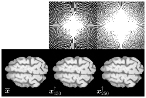
Figure 2: (top) Examples of masks ${\mathb{M}}$ with $M_{a}=150$ and $M_{a}=250$ angles (i.e., $M/N=0.52$ and $M/N=0.76$), respectively. (bottom) Ground truth ($N=128\times 128$), and MAP estimates for $\mathrm{iSNR}=30$ dB.

V An Inpainting CNN

V-A Proposed network architecture

A wealth of architectures and training regimes are available to perform image inpainting [42, 44, 43]. In this work, due to the form of Algorithm 3 that requires to differentiate $h$ (and hence the NN ${\mathcal{G}}$) at each iteration, we propose to use a CNN with fairly simple architecture. In particular, we choose ${\mathcal{G}}$ to be a modified DnCNN, which contains both convolutions and gated convolutions [43, 49]. The architecture is depicted in Figure 1. It is divided into an initial block of $5$ standard convolutional layers and a second block of $5$ gated convolutional layers, each with $128\times 5\times 5$ filters. The network ${\mathcal{G}}$ takes as an input both the mask ${\mathb{M}}$ and an image ${\mathb{x}}$ to be inpainted, in the area identified by the mask. The output is an inpainted image satisfying ${\mathb{M}}^{c}{\mathcal{G}}({\mathb{x}})={\mathb{M}}^{c}{\mathb{x}}$ and such that ${\mathb{M}}{\mathcal{G}}({\mathb{x}})$ corresponds to an inpainted version of ${\mathb{M}}{\mathb{x}}$.

Gated convolutions are modified convolutional layers allowing for inpainting holes of any shape and without specifying those pixels to be inpainted [43]. Where a standard convolution is computed with respect to the uniform measure, a gated convolution is a convolution that is computed with respect to a measure which is itself computed by a learnable convolutional layer, and depends on the input variable. The non-uniform measure is constrained to take values in $C=[0,1]$ and can be interpreted as a level of trust for each pixel.

We propose a DnCNN-based architecture, split into two blocks: a first denoising block to improve robustness, and a second block using gated convolutions aiming to perform the inpainting operation.

V-B Training procedure

For network training, we adopt an approach similar to [42]. Precisely, the network ${\mathcal{G}}$ is trained by minimizing a composite loss function comprising of five terms: an $\ell^{2}$-loss, an $\ell^{1}$ loss restricted to the inpainted region, a TV term restricted to the mask boundary and a perceptual and style loss using the VGG16 feature extractor [50]. Furthermore, we use activation dropouts on the first four layers. We use a dataset containing $90,885$ images and masks prepared from the BRATS21 dataset [51, 52, 53]. Images are preprocessed with additive random noise and random rotations. Masks are preprocessed from the label data, and are randomly dilated. Multiple masks are multiplied to form a new single mask. The processed images are randomly cropped to $96\times 96$ and masked using a randomly chosen mask from our processed mask dataset. The model is trained with the ADAM optimizer, for 32 epochs with a batchsize of 24. The learning rate is $10^{-3}$, dropping to $2\times 10^{-4}$ after 16 epochs. Training was performed with PyTorch, on an NVIDIA GeForce RTX 2080 Ti and lasted 16 hours.

VI Experiments

All our experiments are coded with Pytorch, and performed on an NVIDIA GeForce RTX 2080 Ti.

VI-A Simulation setting

We simulate measurement data by considering the linear sensing model given in (1). We consider images from the BRATS21 dataset [51, 52, 53], cropped to dimension $N=128\times 128$. The forward operator, denoted by ${\boldsymbol{\Phi}}_{M_{a}}$, corresponds to a subsampling 2D Fourier measurement operator. The subsampling operator is a binary mask whose non-zero entries correspond to those pixels lying on a given number of lines, each of which contain the origin and are equally rotationally-spaced. We consider subsampling according to numbers of acquisition angles $M_{a}\in\{150,200,250,300,350\}$, corresponding to ratios $M/N\in\{0.52,0.65,0.76,0.84,0.90\}$. Examples are provided in Figure 2 for $M_{a}=150$ and $M_{a}=250$. We generate the noise ${\mathb{w}}$ for the model (1) as realizations of iid complex Gaussian noise with standard deviation $\delta=M^{-1}\|{\boldsymbol{\Phi}}_{M_{a}}\overline{{\mathb{x}}}\|_{2}10^{-\mathrm{iSNR}/20}>0$, where $\overline{{\mathb{x}}}$ is the ground truth image, for input signal-to-noise ratio (iSNR) values in $\{20,25,30,35\}$ dB. Note that small $\mathrm{iSNR}$ values corresponds to noise with large standard deviation value. Those simulated measurements are processed to compute a MAP estimate ${\mathb{x}}^{\dagger}$, which is a solution to (2), obtained using Algorithm 1. Example MAP estimates are given in Figure 2.

Thereafter, structures of interest are identified manually and expressed as a binary mask ${\mathb{M}}\in\{0,1\}^{N}$. The MAP estimate ${\mathb{x}}^{\dagger}$ and the mask ${\mathb{M}}$ are passed as inputs to Algorithm 3 to quantify uncertainty on structures of interest.

VI-B Algorithm parameters

To implement Algorithm 3, the stepsizes must satisfy (12), that necessitates to compute the Lipschitz constant $\beta$ of $\nabla h$. To do so, we approximate $\beta$ as $\beta\approx\max_{1\leqslant i\leqslant I}\|\nabla h({\mathcal{G}}({\mathb{x}}^{\dagger})+{\boldsymbol{\omega}}_{i})\|_{S}$, where $({\boldsymbol{\omega}}_{i})_{1\leqslant i\leqslant I}$ are realizations of random Gaussian variables with standard deviation $\varsigma=0.01$. In practice, we chose $I=4$, and we compute $\nabla h({\mathb{x}}^{\dagger})$ by automatic differentiation. We then compute $\|\nabla h({\mathcal{G}}({\mathb{x}}^{\dagger})+{\boldsymbol{\omega}}_{i})\|_{S}^{2}$ by power iterations [22].

Note that, according to Definition III.2, for every ${\mathb{x}}\in\mathbb{R}^{N}$, ${\mathcal{G}}({\mathcal{G}}({\mathb{x}}))={\mathcal{G}}({\mathb{x}})$. That is, $h({\mathcal{G}}({\mathb{x}}))=0$, and hence $\nabla h({\mathcal{G}}({\mathb{x}}))=0$. Since we propose to define ${\mathcal{S}}$ using a CNN, we may have poor control over $\nabla h$ in general. However, since we aim to find an element of ${\mathcal{S}}$, if we initialize Algorithm 3 with ${\mathb{x}}^{(0)}={\mathcal{G}}({\mathb{x}}^{\dagger})\in{\mathcal{S}}$, and choose a sufficiently small primal stepsize $\sigma$, we aim to keep our primal steps small, so that each ${\mathb{x}}^{(k)}$ is sufficiently similar to the training dataset.

We consider that the algorithm has converged when

$${\mathb{x}}^{(k)}\in{\widetilde{\mathcal{C}}_{\alpha}}\text{ and }\|{\mathb{x}}^{(k+1)}-{\mathb{x}}^{(k)}\|\leqslant 10^{-3}\|{\mathb{x}}^{(k)}\|,$$ (13)

where $({\mathb{x}}^{(k)})_{k\in\mathbb{N}}$ are the iterates generated by Algorithm 3.

Figure 3: Example where the structure of interest is located near an edge (for $M_{a}=150$, $\mathrm{iSNR}=30$ dB, with $\rho_{\alpha}=0.46$). Grayscale images show (left to right, top to bottom) the MAP ${\mathb{x}}^{\dagger}$, the inpainted MAP ${\mathcal{G}}({\mathb{x}}^{\dagger})$, the output of the proposed PnP-BUQO ${\mathb{x}}^{\ddagger}$ and its inpainted version ${\mathcal{G}}({\mathb{x}}^{\ddagger})$. Color images show differences of images on horizontal and vertical axis, in log scale.

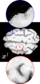
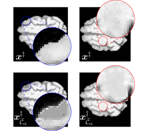
Figure 4: Comparison of BUQO with PnP-BUQO. (left) MAP ${\mathb{x}}^{\dagger}$ ($M_{a}=200,\mathrm{iSNR}=20$ dB). (center & right) Results for two structures, obtained with (top) PnP-BUQO ${\mathb{x}}^{\ddagger}$, ($\rho_{\alpha}=0.018,\rho_{\alpha}=0.018$) and (bottom) BUQO ${\mathb{x}}_{\widetilde{\mathcal{C}}_{\alpha}}^{\ddagger}$ ($\rho_{\alpha}=0.018,\rho_{\alpha}=0.017$). In all instances, $\rho_{\alpha}<\tau$, so $H_{0}$ is rejected.

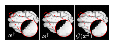
Figure 5: (left) MAP (for $M_{a}=150$, iSNR=$25$ dB) with a checkerboard structure of interest. (center) PnP-BUQO output ${\mathb{x}}^{\ddagger}$ and (right) inpainted output, with $\rho_{\alpha}=0.018$.

VI-C Result interpretation

To evaluate our hypothesis test, it suffices to determine whether or not the sets ${\mathcal{S}}$ and ${\widetilde{\mathcal{C}}_{\alpha}}$ are disjoint, using Corollary III.3. Let ${\mathb{x}}^{\ddagger}$ be the limit point of Algorithm 3. Due to numerical error when running Algorithm 3, and stopping conditions (13), it is not reasonable to ever expect $\|{\mathb{x}}^{\ddagger}-{\mathcal{G}}({\mathb{x}}^{\ddagger})\|=0$ in practice. Thus, as proposed in [33], to interpret the output of Algorithm (3), we introduce the quantity

$$\rho_{\alpha}=\frac{\|{\mathb{x}}^{\ddagger}-{\mathcal{G}}({\mathb{x}}^{\ddagger})\|}{\|{\mathb{x}}^{\dagger}-{\mathcal{G}}({\mathb{x}}^{\dagger})\|}\in[0,1],$$

which is the distance from ${\mathb{x}}^{\ddagger}$ to a fixed point of ${\mathcal{G}}$, normalized with respect to the initial distance. The quantity $\rho_{\alpha}$ can be interpreted as an upper bound on the percentage of the energy of the structure that is supported by the data. Note that the greater the value of $\rho_{\alpha}$, the more confidence we have in rejecting the null hypothesis. Hence $\rho_{\alpha}$ acts similarly to a p-value in classical hypothesis testing.

To decide whether $\|{\mathb{x}}^{\ddagger}-{\mathcal{G}}({\mathb{x}}^{\ddagger})\|$ is large enough to reject the null hypothesis, we consider a tolerance parameter $1\gg\tau>0$ for $\rho_{\alpha}$. If $\rho_{\alpha}>\tau$ then ${\mathcal{S}}\cap{\widetilde{\mathcal{C}}_{\alpha}}={\varnothing}$ and the null hypothesis $H_{0}$ can be rejected with confidence $\alpha$ (see Section III for more details). Otherwise, $\rho_{\alpha}\leqslant\tau$ and we conclude that there is a structure-free image which is concurrent with the observed data. Hence the data are inconclusive and the null hypothesis cannot be rejected.

In our simulations, we choose $\alpha=0.01$ and $\tau=0.02$.

VI-D Results

Qualitative results (True structures)

Figure 3 illustrates the output from PnP-BUQO for an edge structure existing in the ground truth image, for which the data are inconclusive to reject the hypothesis, corresponding to $M_{a}=150$ and iSNR=$30$ dB. Figure 3 shows the MAP estimate ${\mathb{x}}^{\dagger}$ and its structure-free version ${\mathcal{G}}({\mathb{x}}^{\dagger})$, and the PnP-BUQO output ${\mathb{x}}^{\ddagger}$ and its structure-free version ${\mathcal{G}}({\mathb{x}}^{\ddagger})$. An example where the hypothesis is rejected for the same structure, for $M_{a}=200$ and $\mathrm{iSNR}=20$ dB, is shown in Figure 4.

Qualitative results (Artifacts)

The proposed method is able to identify genuine reconstruction artifacts. Indeed, in Figure 5 the MAP contains a checkerboard feature, which is not present in the ground truth. For this feature, simulations with $M_{\alpha}\in\{150,200,250,300,350\}$ all resulted in $\rho_{\alpha}\leqslant\tau$, rejecting the null hypothesis and ensuring that the structure is an artifact.

Qualitative results (Comparison with original BUQO)

We compare the qualitative fidelity of the structure-free image ${\mathcal{G}}({\mathb{x}}^{\ddagger})$ obtained with the proposed PnP-BUQO, with the results obtained with original BUQO [33], for two structures, shown in Figure 4. The central images show an example structure where the original BUQO provides an image in ${\widetilde{\mathcal{C}}_{\alpha}}$ that looks unnatural (dark patch in the inpainted region). In comparison, the proposed PnP-BUQO gives a more natural image. The right images show an example structure where the original BUQO performs better. Nevertheless, we can still observe a patchy texture in the inpainted region. The result obtained by the original BUQO appears unnaturally smooth due to the bounded energy term which defines the space of structure-free images. In contrast, our new method provides an alternative image with a “natural” appearance.

Quantitative results

Figure 6 illustrates the relationship between $\mathrm{iSNR}$ (i.e. noise level), the number of acquisition angles $M_{\alpha}$ and statistic $\rho_{\alpha}$. We observe that confidence in the presence of a structure increases monotonically with respect to both the number of acquisition angles and $\mathrm{iSNR}$.

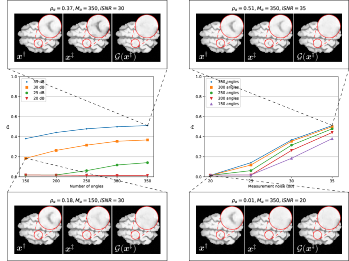
Figure 6: Structure confidence $\rho_{\alpha}$ (for a particular structure) with respect to the number of measurement angles, $M_{a}$ (left) and the iSNR values (right).

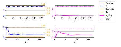
Figure 7: Supporting data for experiments summarized in Figure 6 with $(M_{\alpha},\mathrm{iSNR})=(350,20),(350,35)$, respectively. These plots illustrate the data fidelity $f_{\mathb{y}}({\boldsymbol{\Phi}}{\mathb{x}}^{(k)})$, regularization $g({\mathb{x}}^{(k)})$ and objective $h({\mathb{x}}^{(k)})$.

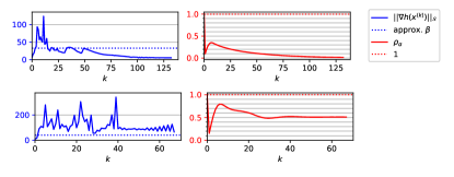
Figure 8: Supporting data for experiments summarized in Figure 6 with $(M_{\alpha},\mathrm{iSNR})=(350,20),(350,35)$, respectively. These plots illustrate $\rho_{\alpha}({\mathb{x}}^{(k)})=\sqrt{h({\mathb{x}}^{(k)})/h({\mathb{x}}^{\dagger})}$ and the norm of the gradient, $\|\nabla h({\mathb{x}}^{(k)})\|_{S}$.

Robustness

Figures 7 and 8 show different curves to illustrate the convergence behaviour of the proposed PnP-BUQO, for representative examples associated with experiments described in Figure 6. Top (resp. bottom) plots correspond to the case $(M_{a},\mathrm{iSNR})=(350,20)$ (resp. $(M_{a},\mathrm{iSNR})=(350,35)$). In Figure 7, we show the convergence behavior of PnP-BUQO for constraints associated with ${\widetilde{\mathcal{C}}_{\alpha}}$ (left plots), and for function $h$ (right plots). In Figure 8, we show the evolution of $\|\nabla h({\mathb{x}}^{(k)})\|_{S}$ with iterations $k$ compared with the approximated estimation of $\beta$ used to choose the stepsizes in Algorithm 3 (left plot), and the evolution of the quantity $\rho_{\alpha}({\mathb{x}}^{(k)})=\sqrt{h({\mathb{x}}^{(k)}/h({\mathb{x}}^{\dagger})}$ (right plot).

VI-E Complexity

In our experiments, due to differentiating network ${\mathcal{G}}$ at each iteration, the proposed PnP-BUQO was slower than the original BUQO algorithm, when run on a unique structure. A quantitative comparison of the time complexity is presented in Table I, for a particular structure of size $N_{M}=170$ pixels. For this example, in total, PnP-BUQO was 4 times slower than BUQO. Note that similar observations were made in [15] for a PnP algorithm where the involved NN also requires back-propagation at each iteration.

However, as already emphasized in previous sections, the original BUQO requires an ad hoc inpainting operator to be built per mask. In addition, the linear operator associated with the mask is built using a greedy approach, and hence its computation does not scale well with the size of the structure. In contrast, the proposed PnP-BUQO uses the same network for any mask, that does not need to be retrained.

Note that choosing stepsizes for Algorithm 3 requires an approximation of $\beta$, as discussed in Section VI-B, that incurs significant computational cost. However, the proposed approximate computation of $\beta$ only depends on the mask ${\mathb{M}}$, and hence does not vary much for masks of similar size. So the approximation of $\beta$ can be computed in advance and used to perform multiple hypothesis tests.

Overall, despite a significant increase in computation time per iteration for the proposed PnP-BUQO, removing the need to compute an ad hoc linear inpainting operator and ignoring the cost of approximating $\beta$ would result in similar overall runtimes for BUQO and PnP-BUQO on average.

Table I: Average computation time ($\pm$ std) for a structure containing $170$ pixels.

	BUQO	PnP-BUQO
$\beta$ approximation per sample (s)	N/A	$4.3\pm 1.9$
Linear operator (s)	$3.6\pm 0.2$	N/A
Per iteration (ms)	$5.6\pm 0.7$	$19.7\pm 2.2$
$\nabla h$ computation (ms)	N/A	$15.2\pm 1.8$
Algorithm runtime (s)	$1.3\pm 1.6$	$3.8\pm 3.5$
Final iteration	$233\pm 297$	$192\pm 176$
Total runtime (s)	$4.9\pm 1.7$	$21.2\pm 8.4$

VII Conclusion

We have proposed a data-driven version of the Bayesian Uncertainty Quantification method proposed in [31, 33]. Precisely, we have designed a plug-and-play algorithm to quantify uncertainty in MAP estimates. The proposed method has been tested on MRI simulations, showing that it leads to more natural explainable images than the original BUQO method.

Allowing ${\mathcal{G}}$ to be an arbitrary operator leaves our framework open to apply in great generality. Moreover, it allows for the user to create custom operators to adapt the definition of ${\mathcal{S}}_{\tau}$ to any particular application.

The time complexity of Algorithm 3 may be reduced by removing backpropogation, as in [15], or using a more lightweight NN, which preserves robustness and fidelity.

While our simulations are demonstrated on MRI brain scans, our abstract formulation for PnP-BUQO applies more generally. Our proposed PnP approach to scalable uncertainty quantification would apply equally well to astronomical imaging, for example, where we must consider very high dimensional data. In such a setting, the time to compute the linear inpainting operator for BUQO is considerable such that a plug-and-play approach would be advantageous [54].

References

- [1] S. Mallat, A Wavelet Tour of Signal Processing (Third Edition). Boston: Academic Press, 2009.
- [2] I. Daubechies, Ten Lectures on Wavelets. Society for Industrial and Applied Mathematics, 1992.
- [3] A. Beck and M. Teboulle, “A fast iterative shrinkage-thresholding algorithm for linear inverse problems,” SIAM J. Imaging Sci., vol. 2, pp. 183–202, 2009.
- [4] P. L. Combettes and J.-C. Pesquet, “Proximal splitting methods in signal processing,” in Fixed-Point Algorithms for Inverse Problems in Science and Engineering, 2009.
- [5] S. P. Boyd, N. Parikh, E. K. wah Chu, B. Peleato, and J. Eckstein, “Distributed optimization and statistical learning via the alternating direction method of multipliers,” Found. Trends Mach. Learn., vol. 3, pp. 1–122, 2011.
- [6] A. Chambolle and T. Pock, “A first-order primal-dual algorithm for convex problems with applications to imaging,” J. Math. Imaging Vision, vol. 40, no. 1, pp. 120–145, 2011.
- [7] L. Condat, “A primal-dual splitting method for convex optimization involving Lipschitzian, proximable and linear composite terms,” J. Optim. Theory Appl., vol. 158, no. 2, pp. 460–479, 2013.
- [8] B. C. Vu, “A splitting algorithm for dual monotone inclusions involving cocoercive operators,” Adv. Comput. Math., vol. 38, no. 3, pp. 667–681, 2013.
- [9] P. Ochs, T. Brox, and T. Pock, “iPiasco: inertial proximal algorithm for strongly convex optimization,” J. Math. Imaging Vision, vol. 53, no. 2, pp. 171–181, 2015.
- [10] E. Chouzenoux, J.-C. Pesquet, and A. Repetti, “Variable metric forward-backward algorithm for minimizing the sum of a differentiable function and a convex function,” J. Optim. Theory Appl., vol. 162, no. 1, pp. 107–132, 2014.
- [11] J.-C. Pesquet and A. Repetti, “A class of randomized primal-dual algorithms for distributed optimization,” J. Nonlinear Convex Anal., vol. 16, no. 12, pp. 2453–2490, 2015.
- [12] H. H. Bauschke and P. L. Combettes, Convex analysis and monotone operator theory in Hilbert spaces, ser. CMS Books in Mathematics/Ouvrages de Mathématiques de la SMC. Springer, New York, 2011, with a foreword by Hédy Attouch.
- [13] K. Zhang, W. Zuo, S. Gu, and L. Zhang, “Learning deep cnn denoiser prior for image restoration,” in 2017 IEEE Conference on Computer Vision and Pattern Recognition (CVPR), 2017, pp. 2808–2817.
- [14] K. Zhang, W. Zuo, and L. Zhang, “Deep plug-and-play super-resolution for arbitrary blur kernels,” in Proceedings of the IEEE/CVF Conference on Computer Vision and Pattern Recognition (CVPR), June 2019.
- [15] S. Hurault, A. Leclaire, and N. Papadakis, “Gradient step denoiser for convergent plug-and-play,” 2021, Preprint 2021, arXiv:2110.03220.
- [16] S. Lunz, O. Öktem, and C.-B. Schönlieb, “Adversarial regularizers in inverse problems,” in Advances in Neural Information Processing Systems, S. Bengio, H. Wallach, H. Larochelle, K. Grauman, N. Cesa-Bianchi, and R. Garnett, Eds., vol. 31. Curran Associates, Inc., 2018.
- [17] R. Ahmad, C. Bouman, G. Buzzard, S. Chan, S. Liu, E. Reehorst, and P. Schniter, “Plug-and-play methods for magnetic resonance imaging: Using denoisers for image recovery,” IEEE Signal Process. Mag., vol. 37, pp. 105–116, 01 2020.
- [18] E. Ryu, J. Liu, S. Wang, X. Chen, Z. Wang, and W. Yin, “Plug-and-play methods provably converge with properly trained denoisers,” in Proceedings of the 36th International Conference on Machine Learning, ser. Proceedings of Machine Learning Research, K. Chaudhuri and R. Salakhutdinov, Eds., vol. 97. PMLR, 09–15 Jun 2019, pp. 5546–5557.
- [19] M. Terris, A. Repetti, J.-C. Pesquet, and Y. Wiaux, “Building firmly nonexpansive convolutional neural networks,” in IEEE International Conference on Acoustics, Speech and Signal Processing (ICASSP 2020), 2020, pp. 8658–8662.
- [20] ——, “Enhanced convergent PNP algorithms for image restoration,” in IEEE International Conference on Image Processing (ICIP 2021), Aug. 2021.
- [21] J. Hertrich, S. Neumayer, and G. Steidl, “Convolutional proximal neural networks and plug-and-play algorithms,” Linear Algebra Appl., vol. 631, pp. 203–234, 2021.
- [22] J.-C. Pesquet, A. Repetti, M. Terris, and Y. Wiaux, “Learning maximally monotone operators for image recovery,” SIAM J. Imaging Sci., vol. 14, no. 3, pp. 1206–1237, 2021.
- [23] A. Repetti, M. Terris, Y. Wiaux, and J.-C. Pesquet, “Dual forward-backward unfolded network for flexible plug-and-play,” in 30th European Signal Processing Conference 2022, Oct. 2022, pp. 957–961.
- [24] C. P. Robert, The Bayesian choice, 2nd ed., ser. Springer Texts in Statistics. Springer, New York, 2007, from decision-theoretic foundations to computational implementation.
- [25] C. P. Robert and G. Casella, Monte Carlo statistical methods, 2nd ed., ser. Springer Texts in Statistics. Springer-Verlag, New York, 2004.
- [26] M. Pereyra, “Proximal Markov chain Monte Carlo algorithms,” Stat. Comput., vol. 26, no. 4, pp. 745–760, 2016.
- [27] M. Pereyra, L. V. Mieles, and K. C. Zygalakis, “Accelerating proximal markov chain Monte Carlo by using an explicit stabilized method,” SIAM J. Imaging Sci., vol. 13, no. 2, pp. 905–935, 2020.
- [28] V. De Bortoli, A. Durmus, M. Pereyra, and A. F. Vidal, “Efficient stochastic optimisation by unadjusted Langevin Monte Carlo. Application to maximum marginal likelihood and empirical Bayesian estimation,” Stat. Comput., vol. 31, no. 3, pp. Paper No. 29, 18, 2021.
- [29] M. Vono, N. Dobigeon, and P. Chainais, “Asymptotically exact data augmentation: models, properties, and algorithms,” J. Comput. Graph. Statist., vol. 30, no. 2, pp. 335–348, 2021.
- [30] P.-A. Thouvenin, A. Repetti, and P. Chainais, “A distributed Gibbs sampler with hypergraph structure for high-dimensional inverse problems,” Université de Lille and Heriot-Watt University, Tech. Rep., Oct. 2022, arXiv.2210.02341.
- [31] A. Repetti, M. Pereyra, and Y. Wiaux, “Uncertainty quantification in imaging: When convex optimization meets Bayesian analysis,” in 26th European Signal Processing Conference (EUSIPCO 2018), Dec. 2018, pp. 2668–2672.
- [32] M. Pereyra, “Maximum-a-posteriori estimation with Bayesian confidence regions,” SIAM J. Imaging Sci,, vol. 10, no. 1, pp. 285–302, 2017.
- [33] A. Repetti, M. Pereyra, and Y. Wiaux, “Scalable Bayesian uncertainty quantification in imaging inverse problems via convex optimization,” SIAM J. Imaging Sci., vol. 12, no. 1, pp. 87–118, 2019.
- [34] X. Cai, M. Pereyra, and J. D. McEwen, “Uncertainty quantification for radio interferometric imaging – I. Proximal MCMC methods,” Mon. Not. R. Astron. Soc., vol. 480, no. 3, pp. 4154–4169, 07 2018.
- [35] ——, “Uncertainty quantification for radio interferometric imaging: II. MAP estimation,” Mon. Not. R. Astron. Soc., vol. 480, no. 3, pp. 4170–4182, 08 2018.
- [36] A. M. Rambojun, H. Komber, J. Rossdale, J. Suntharalingam, J. C. L. Rodrigues, M. J. Ehrhardt, and A. Repetti, “Uncertainty quantification in CT pulmonary angiography,” 2023, Preprint 2023, arXiv:2301.02467.
- [37] N. Komodakis and J.-C. Pesquet, “Playing with duality: An overview of recent primal-dual approaches for solving large-scale optimization problems,” IEEE Signal Process. Mag., vol. 32, pp. 31–54, 2014.
- [38] I. Daubechies, “Orthonormal bases of compactly supported wavelets,” Comm. Pure Appl. Math., vol. 41, no. 7, pp. 909–996, 1988.
- [39] A. Cohen, I. Daubechies, and J.-C. Feauveau, “Biorthogonal bases of compactly supported wavelets,” Comm. Pure Appl. Math., vol. 45, no. 5, pp. 485–560, 1992.
- [40] I. Daubechies, Ten lectures on wavelets, ser. CBMS-NSF Regional Conference Series in Applied Mathematics. SIAM, Philadelphia, PA, 1992, vol. 61.
- [41] P. L. Combettes and J.-C. Pesquet, “Primal-dual splitting algorithm for solving inclusions with mixtures of composite, Lipschitzian, and parallel-sum type monotone operators,” Set-Valued Var. Anal., vol. 20, no. 2, pp. 307–330, 2012.
- [42] G. Liu, F. A. Reda, K. J. Shih, T.-C. Wang, A. Tao, and B. Catanzaro, “Image inpainting for irregular holes using partial convolutions,” in Computer Vision – ECCV 2018. Springer International Publishing, 2018, pp. 89–105.
- [43] J. Yu, Z. Lin, J. Yang, X. Shen, X. Lu, and T. Huang, “Free-form image inpainting with gated convolution,” in 2019 IEEE/CVF International Conference on Computer Vision (ICCV), 2019, pp. 4470–4479.
- [44] Z. Yan, X. Li, M. Li, W. Zuo, and S. Shan, “Shift-net: Image inpainting via deep feature rearrangement,” in Computer Vision - ECCV 2018 - 15th European Conference, Munich, Germany, September 8-14, 2018, Proceedings, Part XIV, ser. Lecture Notes in Computer Science, V. Ferrari, M. Hebert, C. Sminchisescu, and Y. Weiss, Eds., vol. 11218. Springer, 2018, pp. 3–19.
- [45] C. Saharia, W. Chan, H. Chang, C. A. Lee, J. Ho, T. Salimans et al., “Palette: Image-to-image diffusion models,” 2022.
- [46] J. Z. Yinhuai Wang, Jiwen Yu, “Zero-shot image restoration using denoising diffusion null-space model,” in International Conference on Learning Representations (ICLR), 2023.
- [47] H. Attouch, Jérôme, and B. F. Svaiter, “Convergence of descent methods for semi-algebraic and tame problems: proximal algorithms, forward-backward splitting, and regularized gauss-seidel methods,” Math. Program., vol. 137, no. 1-2, pp. 91–129, Aug. 2011.
- [48] L. Condat, A. Hirabayashi, and Y. Hironaga, “Recovery of nonuniformdirac pulses from noisy linear measurements,” in 2013 IEEE International Conference on Acoustics, Speech and Signal Processing, 2013, pp. 6014–6018.
- [49] K. Zhang, W. Zuo, Y. Chen, D. Meng, and L. Zhang, “Beyond a gaussian denoiser: Residual learning of deep CNN for image denoising,” Trans. Img. Proc., vol. 26, no. 7, p. 3142–3155, jul 2017.
- [50] K. Simonyan and A. Zisserman, “Very deep convolutional networks for large-scale image recognition,” in International Conference on Learning Representations, 2015.
- [51] U. Baid, S. Ghodasara, S. Mohan, M. Bilello, E. Calabrese, E. Colak et al., “The RSNA-ASNR-MICCAI BraTS 2021 benchmark on brain tumor segmentation and radiogenomic classification,” 2021, Preprint 2021, arXiv:2107.02314.
- [52] S. Bakas, H. Akbari, A. Sotiras, M. Bilello, M. Rozycki, J. S. Kirby et al., “Advancing the cancer genome atlas glioma MRI collections with expert segmentation labels and radiomic features,” Sci. Data, vol. 4, no. 1, Sep. 2017.
- [53] B. H. Menze, A. Jakab, S. Bauer, J. Kalpathy-Cramer, K. Farahani, J. Kirby et al., “The multimodal brain tumor image segmentation benchmark (BRATS),” IEEE Trans. Med. Imag., vol. 34, no. 10, pp. 1993–2024, Oct. 2015.
- [54] A. Repetti, M. Pereyra, and Y. Wiaux, “Uncertainty quantification in astro-imaging by optimisation,” in Proceedings of the International BASP Frontiers Workshop 2019, Feb. 2019, international BASP Frontiers workshop 2019.