Automatically identifying ordinary differential equations from data

Abstract

Discovering nonlinear differential equations that describe system dynamics from empirical data is a fundamental challenge in contemporary science. Here, we propose a methodology to identify dynamical laws by integrating denoising techniques to smooth the signal, sparse regression to identify the relevant parameters, and bootstrap confidence intervals to quantify the uncertainty of the estimates. We evaluate our method on well-known ordinary differential equations with an ensemble of random initial conditions, time series of increasing length, and varying signal-to-noise ratios. Our algorithm consistently identifies three-dimensional systems, given moderately-sized time series and high levels of signal quality relative to background noise. By accurately discovering dynamical systems automatically, our methodology has the potential to impact the understanding of complex systems, especially in fields where data are abundant, but developing mathematical models demands considerable effort.

Keywords model selection  $\cdot$ system identification  $\cdot$ sparse regression  $\cdot$ nonlinear dynamics  $\cdot$ data-driven discovery

1 Introduction

Since Newton discovered the second law of motion, scientists have sought to formulate mathematical models in the form of differential equations that accurately represent natural phenomena. In the past half-century, dynamical systems have been employed in various disciplines such as physics [1, 2], chemistry [3], biology [4, 5, 6, 7, 8, 9], neuroscience [10, 11, 12], epidemiology [13, 14], ecology [15, 16] and environmental sciences [17, 18]. Nonetheless, developing these models remains challenging and typically requires considerable effort from specialists in the relevant fields [19, 20].

As early as the 1980s, scientists turned to statistical methods to reverse engineer governing equations for nonlinear systems from data, aiming to automatically discover mathematical models that accurately represent the inherent dynamics [21]. This approach is often referred to as the inverse problem [22] or system identification [23]. Subsequent advances have led to significant progress in identifying differential equations symbolically [24, 25, 26, 27, 28, 29, 30, 31, 32, 33, 34, 35, 36, 37]. One practical method that has emerged from this effort is sparse regression, which eliminates the time-consuming task of determining equations manually [38]. A remarkable breakthrough is the sparse identification of nonlinear dynamics (SINDy) [27], an approach that employs a sparsity-promoting framework to identify interpretable models from data by only selecting the most dominant candidate terms from a high-dimensional nonlinear-function space.

SINDy with AIC, an extension of the original SINDy algorithm, uses a grid of sparsity-promoting threshold parameters in conjunction with the Akaike information criterion (AIC), a statistical method for model comparison, to determine the model that most accurately characterizes the dynamics of a given system [39, 27]. Although this method automates model selection, it encounters several obstacles that limit its practicality. Key challenges include its dependence on prior knowledge of the governing equations for model validation and identification, as well as the requirement for high-quality measurements given its limited capacity to compute optimal numerical derivatives from data. Furthermore, the efficacy of SINDy with AIC has only been demonstrated on data sets generated using specific initial conditions, sufficient observations, and low levels of noise, indicating the need for more comprehensive and rigorous analyses to assess its performance in diverse settings.

Here, we present an algorithm for automatically identifying dynamical systems from data by optimally calculating derivatives and incorporating formal variable selection procedures for model inference and selection. Our method tolerates low to medium levels of noise, requiring only the assumptions of model sparsity and the presence of the governing terms in the design matrix. To demonstrate the effectiveness of our approach, we examine its success rate on synthetic data sets generated from known ordinary differential equations, exploring a range of initial conditions, time series of increasing length, and various noise intensities. Our algorithm automates the discovery of three-dimensional systems more efficiently than SINDy with AIC, achieving higher identification accuracy with moderately-sized data sets and high signal quality.

2 Results

2.1 Modeling systems of ODEs with linear regression

Ordinary differential equations (ODEs) are often used to model dynamical systems in the form of

$$\frac{d}{dt}x_{j}(t)=\dot{x}_{j}(t)=f_{j}(x(t))\qquad j=1,\dotsc,m,$$ (1)

where $x=x(t)$ = $\left(x_{1}(t)\ \ x_{2}(t)\ \cdots\ \ x_{m}(t)\right)^{T}\in\mathbb{R}^{m}$ is a state space vector, and $f(x(t)):\mathbb{R}^{m}\rightarrow\mathbb{R}^{m}$ describes the system’s evolution in time [40]. We approximate the dynamics symbolically by

$$\dot{x}_{j}\approx\theta_{\text{F}}^{T}(x)\beta_{j},\qquad j=1,\dotsc,m,$$ (2)

where $\beta_{j}\in\mathbb{R}^{p}$ is a sparse coefficient vector of system parameters and $\theta_{\text{F}}(x)$ is a feature vector containing $p$ symbolic functions, each representing an ansatz that we can use to describe the dynamics.

To identify the system from data, we first construct a state matrix $\mathbf{\tilde{X}}\in\mathbb{R}^{n\times m}$ from measurements of $x(t)$ taken at times $t_{1},t_{2},...,t_{n}$, then apply the Savitzky-Golay filter [41] to smooth each column $\mathbf{x}_{j}=SG(\mathbf{\tilde{x}}_{j})$ and calculate the derivative $\mathbf{\dot{x}}_{j}$. We next consolidate $\mathbf{X}$ and $\mathbf{\dot{X}}$ and build the block design matrix ${\mathbf{\Theta}(\mathbf{X})\in\mathbb{R}^{n\times p}}$:

$$\mathbf{\Theta}(\mathbf{X})=\begin{pmatrix}\rule[-4.30554pt]{0.5pt}{10.76385pt}&\rule[-4.30554pt]{0.5pt}{10.76385pt}&\rule[-4.30554pt]{0.5pt}{10.76385pt}&&\rule[-4.30554pt]{0.5pt}{10.76385pt}&\rule[-4.30554pt]{0.5pt}{10.76385pt}\\ \mathbf{1}&\mathbf{X}&\mathbf{X}^{[2]}&\cdots&\mathbf{X}^{[d]}&\mathbf{\Phi}(\mathbf{X})\\ \rule[-4.30554pt]{0.5pt}{10.76385pt}&\rule[-4.30554pt]{0.5pt}{10.76385pt}&\rule[-4.30554pt]{0.5pt}{10.76385pt}&&\rule[-4.30554pt]{0.5pt}{10.76385pt}&\rule[-4.30554pt]{0.5pt}{10.76385pt}\par\end{pmatrix},$$ (3)

where $\mathbf{X}^{[i]}$ for $i=1,\dotsc,d$ is a matrix whose column vectors denote all monomials of order $i$ in $x(t)$, and $\mathbf{\Phi}(\mathbf{X})$ can contain nonlinear functions such as trigonometric, logarithmic, or exponential [27].

Finally, we perform a linear regression with the above matrices:

$$\mathbf{\dot{X}}=\mathbf{\Theta}(\mathbf{X}){\mathbf{B}}+\mathbf{E},$$ (4)

where $\mathbf{B}\in\mathbb{R}^{p\times m}$ and $\mathbf{E}\in\mathbb{R}^{n\times m}$ denote the coefficient and residual matrices, respectively.

2.2 Automatic regression for governing equations (ARGOS)

Our approach, ARGOS, aims to automatically identify interpretable models that describe the dynamics of a system by integrating machine learning with statistical inference. As illustrated in Fig. 1, our algorithm comprises several key phases to solve the system in Eq. (4). These include data smoothing and numerical approximation of derivatives, as well as the use of bootstrap sampling with sparse regression to develop confidence intervals for variable selection.

In the first phase, we employ the Savitzky-Golay filter, which fits a low-degree polynomial to a local window of data points, reducing noise in the state matrix and approximating the derivative numerically [41]. To optimize the filter, we set polynomial order $o=4$ and construct a grid of window lengths $l$ [42]. For each column of the noisy state matrix $\mathbf{\tilde{X}}$, we find the optimal $l^{\ast}$ that minimizes the mean squared error between each noisy signal $\mathbf{\tilde{x}}_{j}$ and its smoothed counterpart $\mathbf{x}_{j}$ (Supplementary Algorithm 1).

Following smoothing and differentiation, we construct the design matrix $\mathbf{\Theta}(\mathbf{X})$ with monomials up to the $d$-th degree and extract the columns of $\mathbf{\dot{X}}$ and $\mathbf{B}$ from Eq. (4) to identify the governing equations of each component of the system:

$$\mathbf{\dot{x}}_{j}=\mathbf{\Theta}(\mathbf{X}){\beta_{j}}+\epsilon_{j},\qquad j=1,\dotsc,m.$$ (5)

We then apply either the least absolute shrinkage and selection operator (lasso) [43] or the adaptive lasso [44] during the model selection process (Supplementary Algorithm 2). Both algorithms add the $\ell_{1}$ penalty to the ordinary least squares regression (OLS) estimate, shrinking coefficients to zero. This allows for the selection of the nonzero terms for parameter and model inference.

After identifying an initial sparse regression estimate of $\beta_{j}$ in Eq. (5), we trim the design matrix to include only monomial terms up to the highest-order variable with a nonzero coefficient in the estimate. Using the updated design matrix, we reapply the sparse regression algorithm and employ a grid of thresholds to develop a subset of models, with each model containing only coefficients whose absolute values exceed their respective thresholds. Next, we perform OLS on the selected variables of each subset to calculate unbiased coefficients and determine the point estimates from the regression model with the minimum Bayesian information criterion (BIC) [45]. As a final step, we bootstrap this sparse regression process with the trimmed design matrix to obtain 2000 sample estimates [46]. We then construct 95% bootstrap confidence intervals using these sample estimates and identify a final model consisting of variables whose confidence intervals do not include zero and whose point estimates lie within their respective intervals.

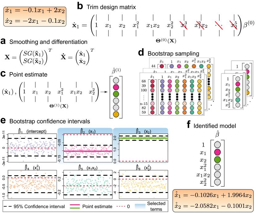
Figure 1: Automatic regression for governing equations (ARGOS). This example illustrates the process of identifying the $\dot{x}_{1}$ equation of a two-dimensional damped oscillator with linear dynamics. We first (a) smooth each noisy state vector in $\mathbf{\tilde{X}}$ and calculate the derivative $\mathbf{\dot{x}}_{1}$ using the Savitzky-Golay filter. Next, we (b) construct the design matrix $\mathbf{\Theta}^{(0)}(\mathbf{X})$, containing the observations $x(t)$ and their interaction terms up to monomial degree $d=5$ —see Eq. (3). Following Eq. (5), we perform sparse regression using either the lasso or the adaptive lasso and determine the highest-order monomial degree with a nonzero coefficient in the estimate $\hat{\beta}^{(0)}$ (in this example, we detect terms up to $d=2$). We then trim the design matrix to include only terms up to this order and (c) perform sparse regression again with the trimmed design matrix and the previously used algorithm (lasso or adaptive lasso), apply OLS on the subset of selected variables, and determine the final $\hat{\beta}^{(1)}$ point estimates. Finally, we (d) employ bootstrap sampling to obtain 2000 sample estimates and (e) develop 95% bootstrap confidence intervals to (f) identify the $\hat{\beta}$ by selecting the coefficients whose intervals contain the point estimate but do not include zero.

2.3 Assessing ARGOS systematically

To evaluate the effectiveness of our approach, we used 100 random initial conditions to expand well-known ODEs and generated data sets with varying time series lengths $n$ and signal-to-noise ratios (SNR) (see Methods). We then introduced a success rate metric, defined as the proportion of instances where an algorithm identified the correct terms of the governing equations from a given dynamical system. This metric allowed us to quantitatively measure the performance of an algorithm across different dynamical systems, as well as different SNR and $n$ values (see Supplementary Tables S1 and S2). Figure 2 highlights success rates exceeding 80%, demonstrating that our method consistently outperformed SINDy with AIC in identifying the underlying system of the data. We accurately represented linear systems with less than 800 data points and medium SNRs, underscoring the method’s ability to handle straightforward dynamics. Notably, even with only moderately-sized data sets or medium SNRs, we successfully identified three out of five of the two-dimensional ODEs using the lasso with ARGOS, showcasing the effectiveness of integrating classic statistical learning algorithms within our framework. The adaptive lasso was able to identify the non-linear ODEs in three dimensions with higher accuracy than the other algorithms tested. These results suggest that the adaptive lasso is suitable for identifying non-linear ODEs in higher dimensional systems.

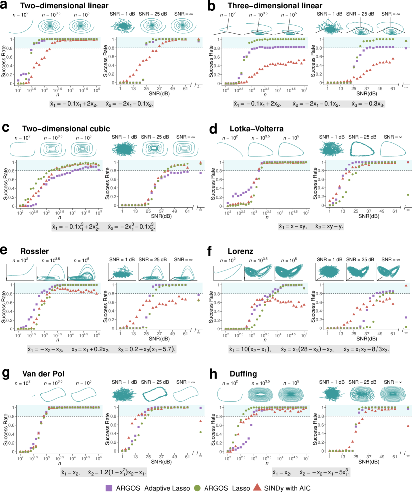
Figure 2: Success rate of ARGOS versus SINDy with AIC for linear and nonlinear systems. We generate 100 random initial conditions and examine the success rate of ARGOS and SINDy with AIC in discovering the correct terms of the governing equations from each system at each value of $n$ and SNR. (a)-(b) Linear systems. First-order nonlinear systems in two (c)-(d) and three (e)-(f) dimensions. (g)-(h) Second-order nonlinear systems. We increase the time-series length $n$ while holding $\text{SNR}=49\ \text{dB}$ (left panels) and fix $n=5000$ when increasing the SNR (right panels). Shaded regions represent model discovery above 80%.

The systematic analysis, presented in Fig. 2, emphasized the efficacy of our approach as $n$ and SNR increased. The importance of data quality and quantity is further supported by Fig. 3, which illustrates the frequency at which our approach identified each term in the design matrix across different values of $n$ and SNR. The boxes in the figure delineate regions where each algorithm achieved model discovery above 80% for the Lorenz system, providing insights into the selected terms contributing to the success and failure of each method across different settings. When faced with limited observations and low signal quality, our approach identified overly sparse models that failed to represent the governing dynamics accurately, while SINDy with AIC selected erroneous terms, struggling to obtain a parsimonious representation of the underlying equations. Figure 3 also illustrates the decline in our method’s performance for deterministic systems, as it identified several ancillary terms for the Lorenz dynamics when $\text{SNR}=\infty$ (additional details for each system are provided in the Supplementary Information). The decrease in identification accuracy stemmed from the identified model’s violation of the homoscedasticity assumption in linear regression, which occurs when residuals exhibit non-constant variance. Figure 4 demonstrates that our method did not satisfy this assumption when identifying the $\dot{x}_{1}$ equation of the Lorenz system. Consequently, our approach selected additional terms to balance the variance among the model’s residuals while sacrificing correct system discovery. As the noise in the system slightly increased, however, homoscedasticity in the residuals became more pronounced, enabling our approach to distinguish the equation’s true underlying structure. Thus, our method proved more practical in accurately identifying the correct terms of the governing equations when data contained low levels of noise in the signal, which is often the case in many real-world applications, as opposed to when dealing with noiseless systems.

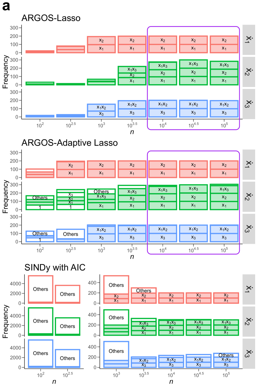
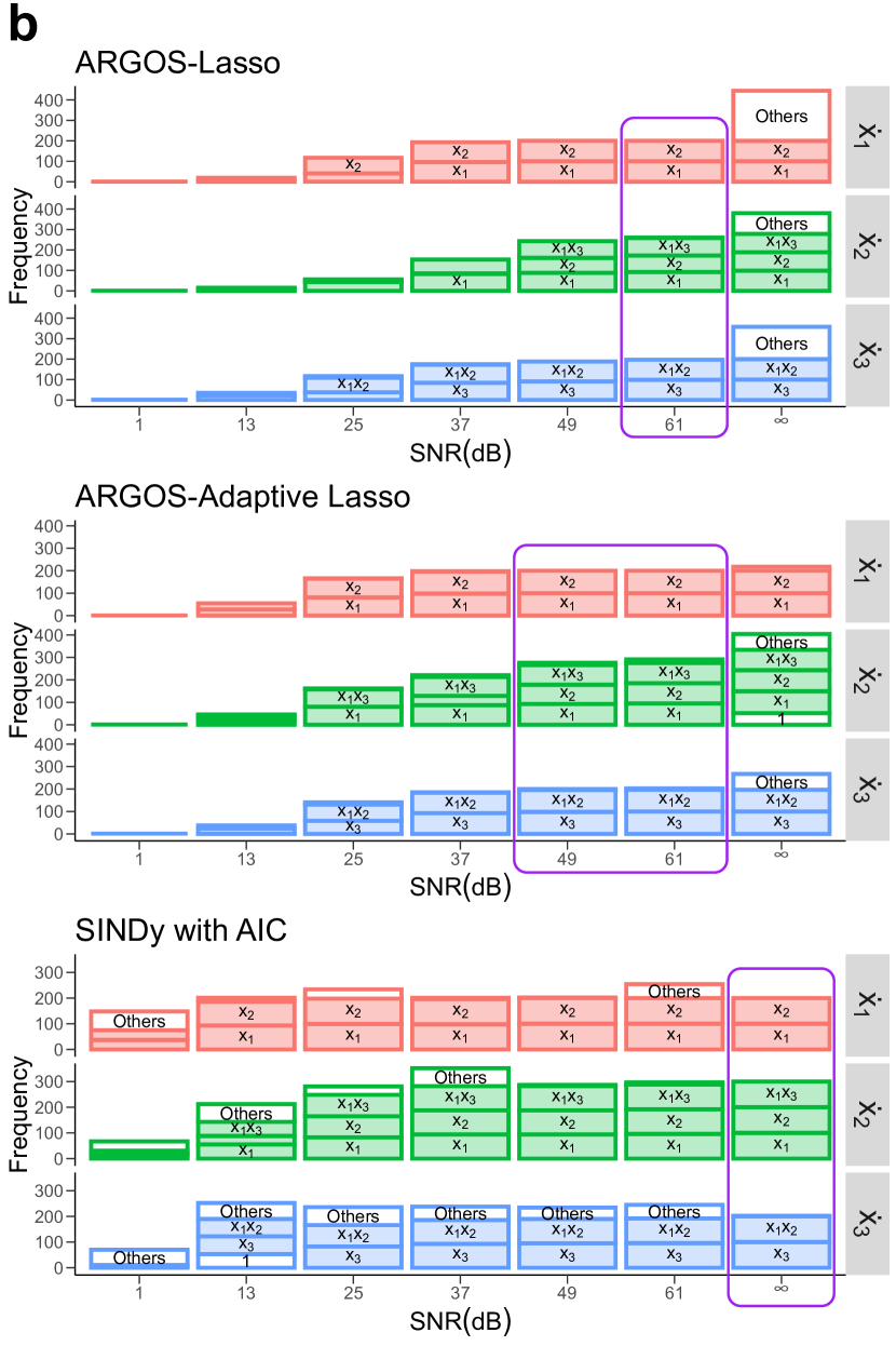
Figure 3: Frequency of identified variables for the Lorenz system across algorithms. Colors correspond to each governing equation; filled boxes indicate correctly identified variables, while white boxes denote erroneous terms. Panels show the frequency of identified variables for data sets with (a) increasing $n$ (SNR = 49 dB), and (b) SNR ($n=5000$). Purple-bordered regions demarcate model discovery above 80%.

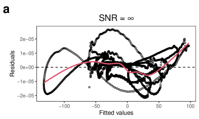
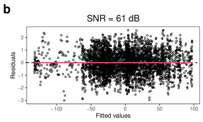
Figure 4: Residuals vs fitted diagnostics for the ARGOS-Lasso identified model of the Lorenz $\dot{x}_{1}$ equation. Comparison of residuals for the prediction models identified using the lasso with ARGOS for the Lorenz system’s $\dot{x}_{1}$ equation when data are (a) noiseless and (b) contaminated by $\text{SNR}=61\ \text{dB}$.

Our method outperformed SINDy with AIC in identifying a range of ODEs, especially three-dimensional systems. One potential explanation for the lesser performance of SINDy with AIC is that multicollinearity in the design matrix often causes OLS to produce unstable coefficients. Due to the sensitivity of the estimated coefficients, small changes in the data can lead to fluctuations in their magnitude, making it difficult for the sparsity-promoting parameter to determine the correct model. As a result, the initial phase of the hard-thresholding procedure of SINDy with AIC inadvertently removed the true dynamic terms of the underlying system. Therefore, this model selection approach will likely face persistent challenges when discovering higher-dimensional systems that contain additional multicollinearity in the design matrix.

Figure 5 shows the computational time, measured in seconds, required for our approach and SINDy with AIC to perform model discovery. While our method demanded greater computational effort for the two-dimensional linear system than SINDy with AIC, it demonstrated better efficiency in identifying the Lorenz dynamics as $n$ increased. The decrease in efficiency of SINDy with AIC can be attributed to its model selection process, which involves enumerating all potential prediction models—a procedure that becomes progressively more expensive with data in higher dimensions [39]. In contrast, our approach displayed a similar rate of increase in computational complexity as the time series expanded for both systems, suggesting that our method was less affected by the growing data dimensionality than SINDy with AIC. Thus, our method offers a more efficient alternative for identifying three-dimensional systems with increasing time series lengths.

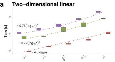
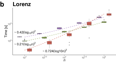
Figure 5: Time-complexity (seconds) between ARGOS and SINDy with AIC. Boxplots depict the computational time required for model discovery over 30 instances for (a) a two-dimensional damped oscillator with linear dynamics and (b) the Lorenz system. The black bar within each box represents the median computational time. Whiskers extending from each box show 1.5 times the interquartile range. Data points beyond the end of the whiskers are outlying points. Equations accompanying the dashed lines indicate the fitted mean computational time for each algorithm at various values of $n$.

3 Discussion

We have demonstrated an automatic method, ARGOS, for extracting dynamical systems from scarce and noisy data without prior knowledge of the governing equations. Our approach combines the Savitzky-Golay filter for signal denoising and differentiation with sparse regression and bootstrap sampling for confidence interval estimation, effectively addressing the inverse problem of inferring underlying dynamics from observational data through reliable variable selection. By examining diverse trajectories, we showcased the capabilities of our algorithm in automating the discovery of mathematical models from data, consistently outperforming the established SINDy with AIC, especially when identifying systems in three dimensions.

While we have shown promising results with our approach, it is important to note several potential limitations. First, although our method effectively automates model discovery, it can only correctly represent the true governing equations if the active terms are present in the design matrix, a constraint inherent in regression-based identification procedures. Building on this point, we stress the importance of data quantity and quality as identification accuracy improved with sufficient observations and moderate to high signal-to-noise ratios. We also found that our method performs better when data contains low levels of noise, as opposed to noiseless systems. The linear regression assumption of homoscedasticity is violated under noiseless conditions, and the method identifies spurious terms to develop a more constant variance among the residuals. However, this issue can be mitigated in the presence of a small amount of noise in the data, leading to a more constant variance in the residuals of the true model and enabling more accurate identification. Lastly, as the number of observations and data dimensionality increase, bootstrap sampling becomes computationally demanding, which can significantly prolong the model selection process and limit our algorithm’s applicability in real-time. Nonetheless, obtaining confidence intervals through bootstrap sampling serves as a reliable approach for our method, allowing us to eliminate superfluous terms and select the ones that best represent the underlying equations, ultimately leading to more accurate predictions of the system’s dynamics.

In this information-rich era, data-driven methods for uncovering governing equations are increasingly crucial in scientific research. By developing automated processes, researchers can develop concise models that accurately represent the underlying dynamics in their data, accelerating advancements across various disciplines in science. Our study endorses an inference-based approach that combines statistical learning and model assessment methods, emphasizing the importance of thorough model evaluation for building confidence in discovering governing equations from data. As data-driven techniques advance, we look forward to further developments in automatic system identification that will continue contributing to the search for the elusive laws governing many intricate systems.

4 Methods

4.1 The lasso and adaptive lasso for variable selection

For the $j$th column of $\mathbf{\dot{X}}$ and $\mathbf{B}$ in Eq. (4), we implement sparse regression by adding weighted $\ell_{q}$ penalties to the OLS regression estimate [47]

$$\operatorname*{\arg\min}_{\beta}\left\{\sum_{i=1}^{n}\left(\dot{x}_{i}-\beta_{0}-\sum_{k=1}^{p}\theta(\mathbf{X})_{i,k}\beta_{k}\right)^{2}+\lambda\sum_{k=1}^{p}w_{k}|\beta_{k}|^{q}\right\}.$$ (6)

When all weights $w_{k}=1$ for $k=1,\dots,p$, Eq. (6) represents the lasso for $q=1$ and ridge regression for $q=2$ [43, 48]. Furthermore, the adaptive lasso is derived from the lasso by incorporating pilot estimates $\tilde{\beta}$ and setting $w_{k}=1/|\tilde{\beta}_{k}|^{\nu}$ [44]. The weighted penalty in the adaptive lasso can be interpreted as an approximation of the $\ell_{p}$ penalties with $p=1-\nu$ [49]. Therefore, fixing $\nu=1$ allows us to achieve a soft-threshold approximation to the $\ell_{0}$ penalty, providing an alternative to the hard-thresholding in the SINDy algorithm, which requires a choice of the cut-off hyperparameter [27].

As $\lambda$ increases in Eq. (6), ridge regression, the lasso, and the adaptive lasso shrink the coefficients toward zero. However, of these three methods, the lasso and the adaptive lasso perform variable selection by reducing small coefficients to exactly zero [43]. We use glmnet to solve Eq. (6) by producing a default $\lambda$ grid and applying 10-fold cross-validation to determine the optimal initial tuning parameter $\lambda_{0}^{\ast}$ [50]. We then refine the grid around $\lambda_{0}^{\ast}$ with 100 points spanning $[\lambda_{0}^{\ast}/10,1.1\cdot\lambda_{0}^{\ast}]$ and impose this updated grid on glmnet to solve Eq. (6) again, identifying the optimal $\lambda^{\ast}$ that best predicts $\mathbf{\dot{x}}_{j}$.

The lasso is effective when only a few coordinates of the coefficients $\beta$ are nonzero. However, like OLS, the lasso provides unstable estimates when predictors are collinear, whereas ridge regression produces more stable solutions when multicollinearity exists in the data [47]. Therefore, we apply ridge regression to the data in the first stage of the adaptive lasso to obtain stable pilot estimates $\tilde{\beta}$ and reduce the effects of multicollinearity [44].

The second stage of the adaptive lasso then uses the $\tilde{\beta}$ pilot estimates to calculate the weights vector $w$, enabling variable selection by solving the problem in Eq. (6). Here, we calculate the weights vector $w$ using pilot estimates $\tilde{\beta}$ corresponding to the optimal $\lambda^{*}_{\text{ridge}}$ ridge regression model before identifying a separate tuning parameter $\lambda^{\ast}_{\text{adaptive lasso}}$. In doing so, we make Eq. (6) less computationally expensive since we optimize twice on a single parameter rather than simultaneously optimizing over $\lambda^{\ast}_{\text{ridge}}$ and $\lambda^{\ast}_{\text{adaptive lasso}}$ [51].

The adaptive lasso often yields a sparser solution than the lasso since applying individual weights to each variable places a stronger penalty on smaller coefficients, reducing more of them to zero. Here, small $\tilde{\beta}$ coefficients from the first stage of the adaptive lasso lead to a larger penalty in the second. Larger penalty terms in the second stage of the adaptive lasso result in more coefficients being set to zero than the standard lasso method. Furthermore, a smaller penalty term enables the adaptive lasso to uncover the true coefficients and reduce bias in the solution [51].

The adaptive lasso, valuable for system identification, obtains the oracle property when the $\tilde{\beta}$ pilot estimates converge in probability to the true value of $\beta$ at a rate of $1/\sqrt{n}$ ($\sqrt{n}$-consistency). As $n$ increases, the algorithm will select the true nonzero variables and estimate their coefficients as if using maximum likelihood estimation [44].

4.2 Algorithm implementation

When applying ARGOS for model selection, we use $\eta=10^{-8},10^{-7},\dotsc,10^{1}$ for thresholding the sparse regression coefficients before performing OLS on each subset ${\mathcal{K}_{i}=\{k:|\hat{\beta}_{k}|\geq\eta_{i}\}},\ i=1,\dotsc,\mathbf{card}(\eta)$ of selected variables, determining an unbiased estimate for $\beta$ [47]. We then calculate the BIC for each $\eta$ regression model and select the model with the minimum value, further promoting sparsity in the identification process [52, 45].

The number of bootstrap sample estimates $B$ must be large enough to develop confidence intervals for variable selection [46]. Therefore, we collect $B=2000$ bootstrap sample estimates and sort them by ${\hat{\beta}_{k}^{\text{OLS}\{1\}}\leq\hat{\beta}_{k}^{\text{OLS}\{2\}}\leq\dots\leq\hat{\beta}_{k}^{\text{OLS}\{B\}}}$. We then use the 100(1 - $\alpha$)$\%$ confidence level, where $\alpha=0.05$, to calculate the integer part of $B\alpha/2$ and develop estimates of the lower and upper bounds: $CI_{\text{lo}}=[B\alpha/2]$ and $CI_{\text{up}}=B-CI_{\text{lo}}+1$. Finally, we implement these calculations to develop confidence intervals $\left[\hat{\beta}_{k}^{\text{OLS}\{CI_{\text{lo}}\}},\hat{\beta}_{k}^{\text{OLS}\{CI_{\text{up}}\}}\right]$ from our sample distribution [53].

We apply our implementation of the Savitzky-Golay filtering method to perform the entire system identification process with SINDy with AIC automatically.

4.3 Building the data sets and tests

We conducted two sets of numerical experiments to assess the impact of data quality and quantity on the performance of the algorithms. To evaluate the algorithms’ performance with limited data, we first kept the signal-to-noise ratio constant ($\text{SNR}=49$) and increased the number of observations $n$ for each ODE system. We generated 100 random initial conditions and used temporal grids starting with $t_{\text{initial}}=0$ and a varying $t_{\text{final}}$ between $1$ ($n=10^{2}$) and $1000$ ($n=10^{5}$) with a time step $\Delta t=0.01$. For the Lorenz equations, we used $\Delta t=0.001$, resulting in $t_{\text{final}}$ values ranging from $0.1$ ($n=10^{2}$) and $100$ ($n=10^{5}$) [27].

To examine the algorithms’ performance under noisy conditions, we varied the SNR in the data by corrupting the state matrix with a zero-mean Gaussian noise matrix $\mathbf{Z}\sim\mathcal{N}(0,\sigma_{\mathbf{Z}}^{2})$. In this setting, we determined the standard deviation $\sigma_{\mathbf{z}_{j}}$ of each column of $\mathbf{Z}$ as

$$\sigma_{\mathbf{z}_{j}}=\sigma_{\mathbf{x}_{j}}\cdot 10^{-\frac{\text{SNR}}{20}},\qquad j=1,\dotsc,m,$$ (7)

and develop the noise corrupted $\tilde{\mathbf{X}}$ as [54]

$$\tilde{\mathbf{X}}=\mathbf{X}+\mathbf{Z}.$$ (8)

Keeping $n$ constant, we again used 100 random initial conditions and generated $\tilde{\mathbf{X}}$ matrices increasing in noise levels such that $\text{SNR}=1,4,\dotsc,61\ \text{dB}$ with $\Delta$SNR = 3 dB, including a noiseless system ($\text{SNR}=\infty$).

For both the tests with varying $n$ and SNR, we constructed the design matrix $\mathbf{\Theta}^{(0)}(\mathbf{X})$ with monomial functions up to $d=5$ of the smoothed columns of $\mathbf{X}$ [27]. We then performed system identification with each data set and calculated the success rate of each algorithm as the probability of extracting the correct terms of the governing equations. Additionally, we analyzed the most frequently selected variables of each method.

Finally, we measured the computational time, in seconds, for running our method and SINDy with AIC by performing model discovery on 30 instances of the two-dimensional linear system and the Lorenz system for time series lengths $n=10^{2},10^{2.5},\dots,10^{5}$, using one CPU core with a single thread.

4.4 Code availability

All code used in this study is available at http://github.com/kevinegan31/ARGOS.

4.5 Data availability

All data generated for this study can be generated with the code available at http://github.com/kevinegan31/ARGOS. We provide a snapshot of the data on GitHub.

S1 Supplementary Information

Table S1: Minimum number of observations ($n$) needed for each method to obtain 80% accuracy in identifying governing equations of dynamical systems. Top-performing algorithms are in red, and three-dimensional systems have a shaded background.

System	Algorithm	$n$
Two-dimensional linear	ARGOS-Lasso	$10^{2.6}\ (399)$
	ARGOS-Adaptive Lasso	$10^{2.6}\ (399)$
	SINDy with AIC	$10^{3.3}\ (1996)$
	ARGOS-Lasso	$10^{2.9}\ (795)$
	ARGOS-Adaptive Lasso	$10^{3.2}\ (1585)$
Three-dimensional linear	SINDy with AIC	NA
Two-dimensional cubic	ARGOS-Lasso	$10^{3.2}\ (1585)$
	SINDy with AIC	$10^{3.3}\ (1996)$
	ARGOS-Adaptive Lasso	$10^{4.1}\ (12590)$
Lotka-Volterra	ARGOS-Adaptive Lasso	$10^{3.2}\ (1585)$
	SINDy with AIC	$10^{3.2}\ (1585)$
	ARGOS-Lasso	$10^{3.3}\ (1996)$
	ARGOS-Adaptive Lasso	$10^{2.9}\ (795)$
	ARGOS-Lasso	$10^{3.2}\ (1585)$
Rossler	SINDy with AIC	$10^{3.2}\ (1585)$
	ARGOS-Adaptive Lasso	$10^{3.8}\ (6310)$
	ARGOS-Lasso	$10^{3.9}\ (7944)$
Lorenz	SINDy with AIC	NA
Van der Pol	ARGOS-Adaptive Lasso	$10^{2.9}\ (795)$
	SINDy with AIC	$10^{2.9}\ (795)$
	ARGOS-Lasso	$10^{3.0}\ (1000)$
Duffing	ARGOS-Lasso	$10^{2.6}\ (399)$
	SINDy with AIC	$10^{2.9}\ (795)$
	ARGOS-Adaptive Lasso	$10^{3.0}\ (1000)$

Table S2: Maximum signal-to-noise ratio (SNR) tolerated by each method to achieve 80% accuracy in identifying the governing equations of the dynamical systems. Top-performing algorithms are in red, and three-dimensional systems have a shaded background.

System	Algorithm	SNR
Two-dimensional linear	ARGOS-Lasso	25
	ARGOS-Adaptive Lasso	25
	SINDy with AIC	37
	ARGOS-Lasso	31
	ARGOS-Adaptive Lasso	40
Three-dimensional linear	SINDy with AIC	$\infty$
Two-dimensional cubic	ARGOS-Lasso	43
	SINDy with AIC	46
	ARGOS-Adaptive Lasso	NA
Lotka-Volterra	ARGOS-Adaptive Lasso	16
	SINDy with AIC	22
	ARGOS-Lasso	28
	ARGOS-Adaptive Lasso	31
	ARGOS-Lasso	34
Rossler	SINDy with AIC	NA
	ARGOS-Adaptive Lasso	46
	ARGOS-Lasso	55
Lorenz	SINDy with AIC	$\infty$
Van der Pol	SINDy with AIC	16
	ARGOS-Adaptive Lasso	19
	ARGOS-Lasso	25
Duffing	ARGOS-Lasso	28
	ARGOS-Adaptive Lasso	28
	SINDy with AIC	34

S2 Linear systems

Two-dimensional damped oscillator with linear dynamics

We examined the two-dimensional linear system as [27]

$$\dot{x}_{1} =-0.1x_{1}+2x_{2},$$ (S1)

$$\dot{x}_{2} =-2x_{1}-0.1x_{2}.$$

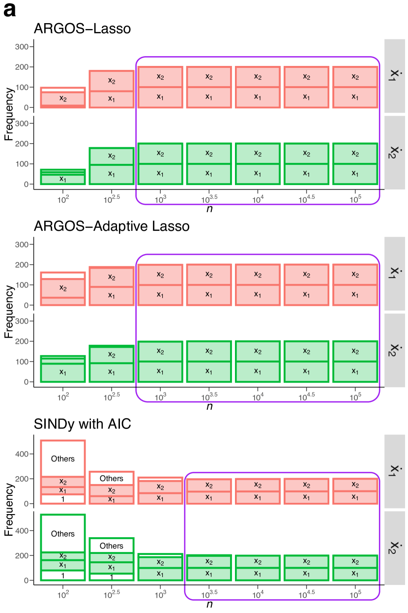
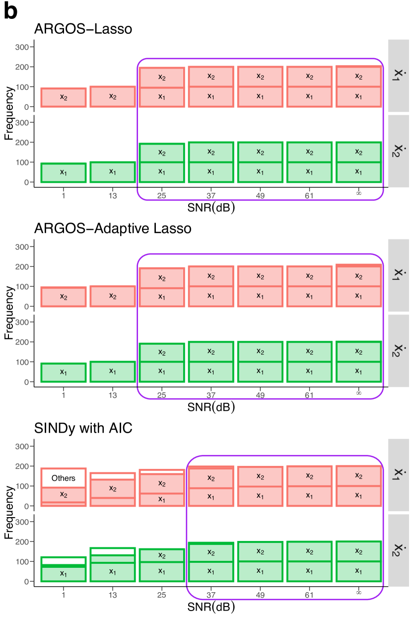
Figure S1: Frequency of identified variables for the two-dimensional damped oscillator with linear dynamics across algorithms. Colors correspond to each governing equation; filled boxes indicate correctly identified variables, while white boxes denote erroneous terms. Panels show the frequency of identified variables for data sets with (a) increasing $n$ (SNR = 49 dB), and (b) SNR ($n=5000$). Purple-bordered regions demarcate model discovery above 80%.

For $x_{1}(t)$ and $x_{2}(t)$, we generated a random uniform distribution of 100 values between $[10^{-1},10^{3}]$.

In Fig. S1, we observe the performance of our approach and SINDy with AIC in discovering the two-dimensional damped oscillator with linear dynamics. We found that with less than 300 observations and low SNR, our method identified overly sparse models and struggled to represent the underlying equations of the system accurately. As the length of the time series $n$ increased and the data became less contaminated with noise, however, the performance of our method improved in extracting the true terms. Conversely, SINDy with AIC demonstrated a tendency to produce dense models, which contained numerous erroneous variables, particularly with less than 1000 observations and low to medium SNR.

Three-dimensional linear system

We evaluated a three-dimensional system [27]:

$$\dot{x}_{1} =-0.1x_{1}+2x_{2},$$ (S2)

$$\dot{x}_{2} =-2x_{1}-0.1x_{2},$$

$$\dot{x}_{3} =-0.3x_{3}.$$

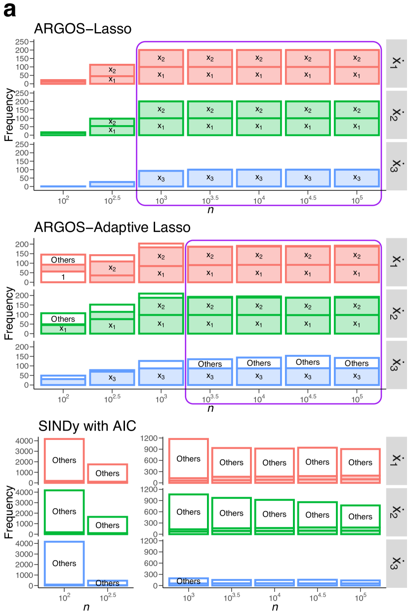
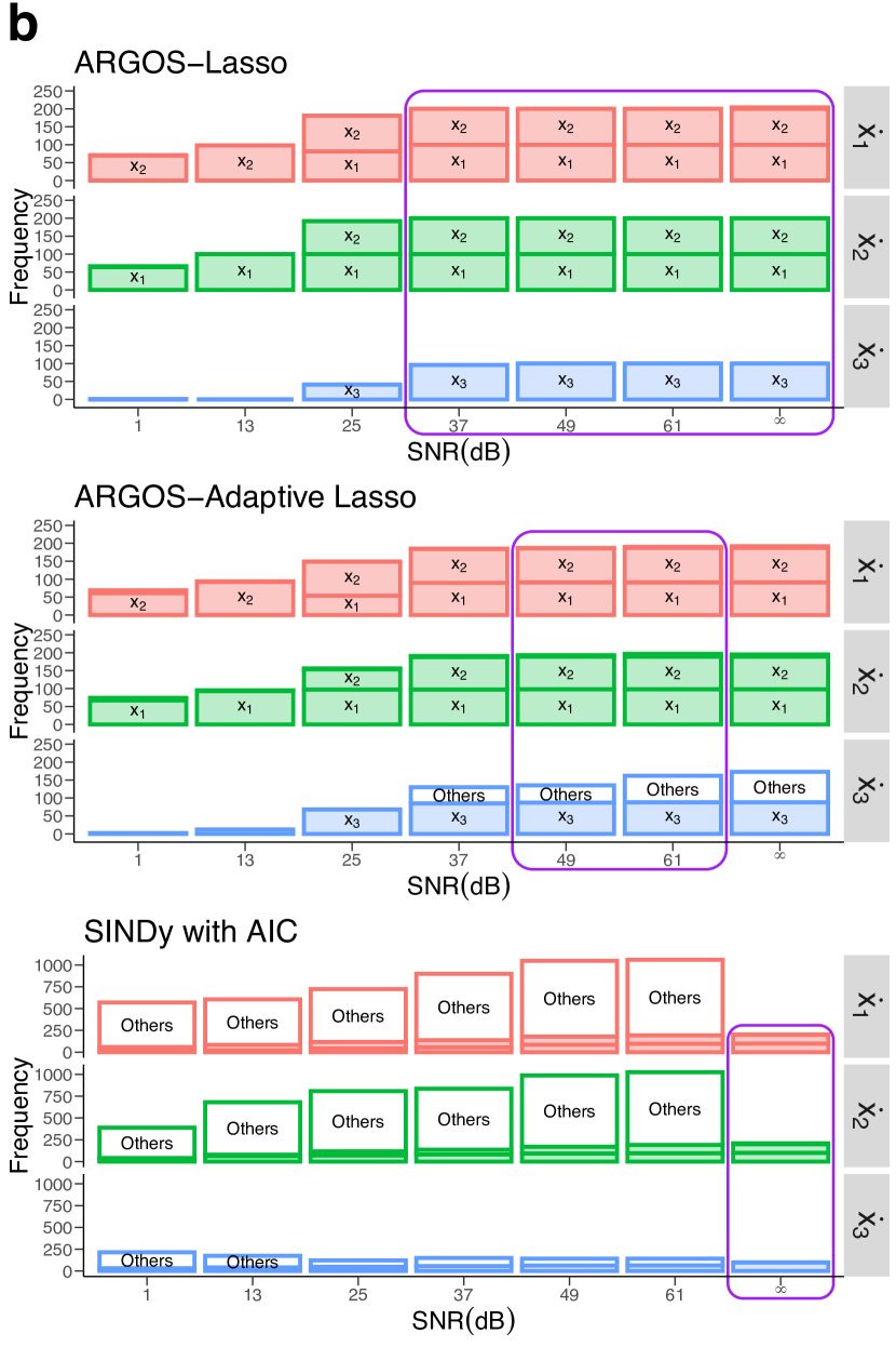
Figure S2: Frequency of identified variables for the three-dimensional linear system across algorithms. Colors correspond to each governing equation; filled boxes indicate correctly identified variables, while white boxes denote erroneous terms. Panels show the frequency of identified variables for data sets with (a) increasing $n$ (SNR = 49 dB), and (b) SNR ($n=5000$). Purple-bordered regions demarcate model discovery above 80%.

For $x_{1}(t)$, $x_{2}(t)$, and $x_{3}(t)$, we again developed a random uniform distribution containing 100 values between $[10^{-1},10^{3}]$.

Figure S2 demonstrates the efficacy of employing the lasso within our framework, as the method more consistently identified the three-dimensional linear system than the other two algorithms studied here. With greater than 1000 observations and medium SNR, our approach accurately represented these simple dynamics. We also found that, with low SNR and less than 300 observations, our method discovered models that were overly sparse and did not fully represent the dynamics, while SINDy with AIC often failed to discover a parsimonious representation of the system by identifying dense models with superfluous terms.

S3 First-order nonlinear systems

Two-dimensional damped oscillator with cubic dynamics

We examined a two-dimensional system with cubic dynamics as [27]

$$\dot{x}_{1} =-0.1x_{1}^{3}+2x_{2}^{3},$$ (S3)

$$\dot{x}_{2} =-2x_{1}^{3}-0.1x_{2}^{3}.$$

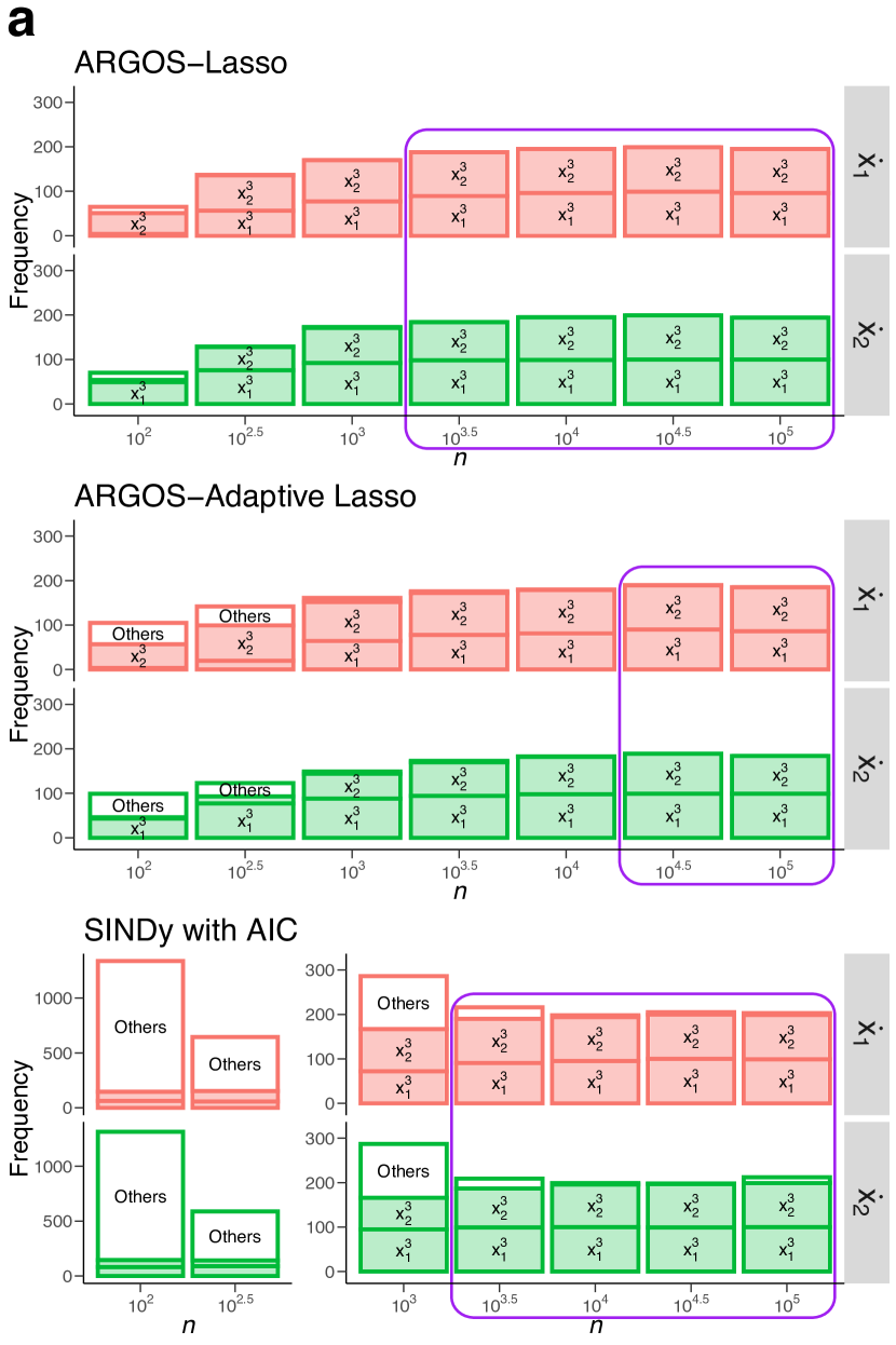
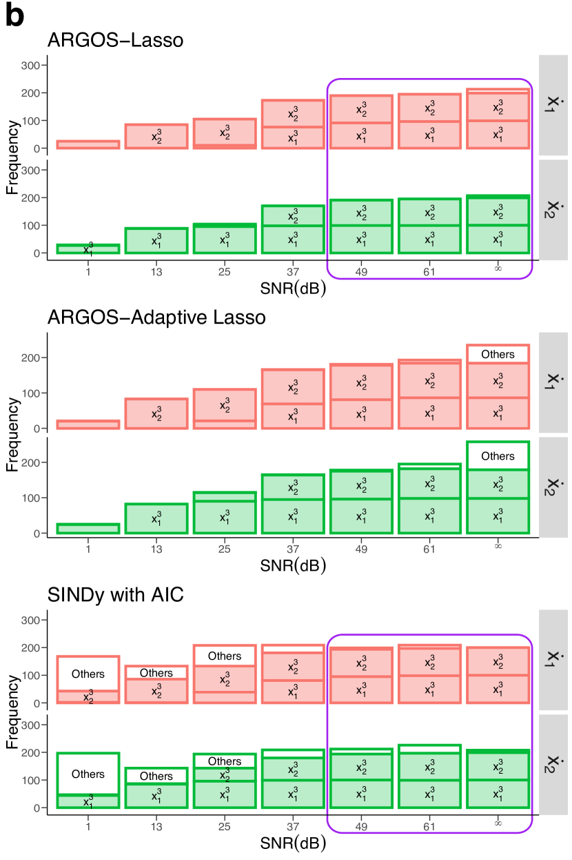
Figure S3: Frequency of identified variables for the two-dimensional damped oscillator with cubic dynamics across algorithms. Colors correspond to each governing equation; filled boxes indicate correctly identified variables, while white boxes denote erroneous terms. Panels show the frequency of identified variables for data sets with (a) increasing $n$ (SNR = 49 dB), and (b) SNR ($n=5000$). Purple-bordered regions demarcate model discovery above 80%.

For $x_{1}(t)$ and $x_{2}(t)$, we generated a random uniform distribution containing 100 values between $[-2,2]$.

Figure S3 further demonstrates the effectiveness of the lasso algorithm for identifying the two-dimensional damped harmonic oscillator with cubic dynamics. Here, SINDy with AIC performed model discovery with similar accuracy to our approach, while both the lasso and SINDy with AIC ultimately outperformed the adaptive lasso.

Lotka-Volterra system

The Lotka-Volterra system is described by two first-order nonlinear differential equations commonly used to depict the interaction dynamics between two species in biological systems, with one being the predator and the other the prey [55]. The predator-prey equations are represented as

$$\dot{x}_{1} =\alpha x_{1}-\zeta x_{1}x_{2},$$ (S4)

$$\dot{x}_{2} =\delta x_{1}x_{2}-\gamma x_{2},$$

where $\alpha=1$ represents the prey birth rate and $\delta=-1$ is the predator death rate, and $\zeta=-1$ and $\gamma=1$ are the interaction parameters [56]. Since the population cannot be negative, we used a random uniform distribution with 100 positive values between $[1,10]$ for the initial conditions of both $x_{1}(t)$ and $x_{2}(t)$.

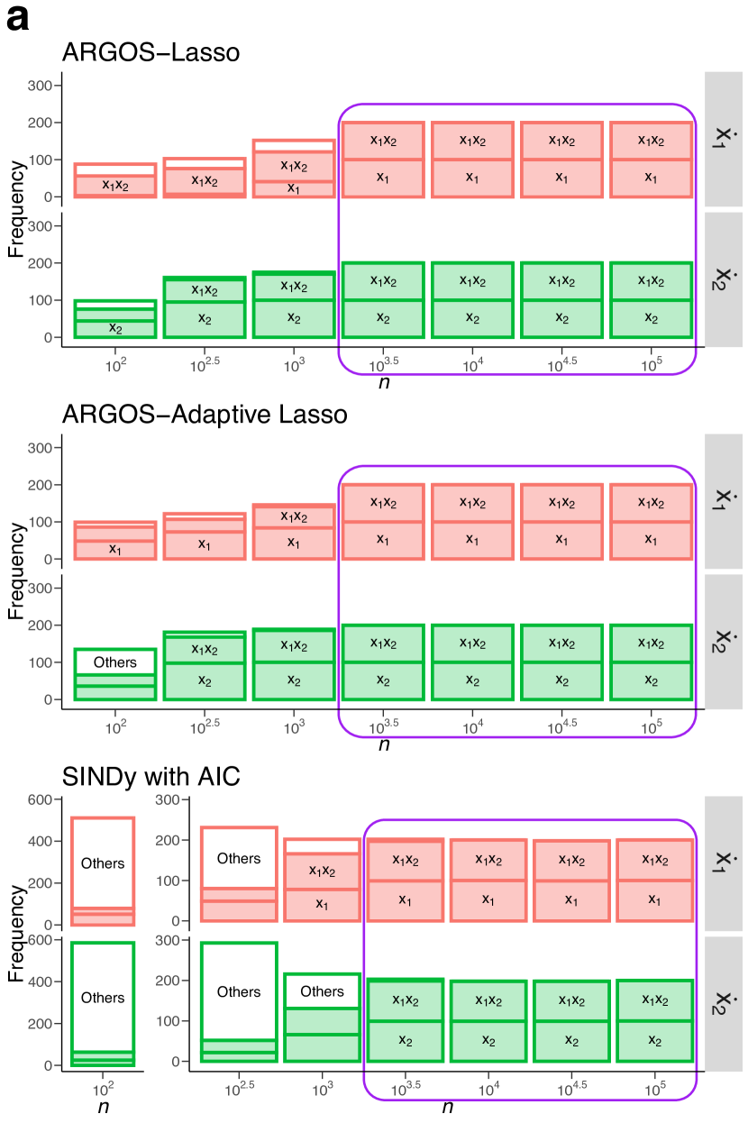
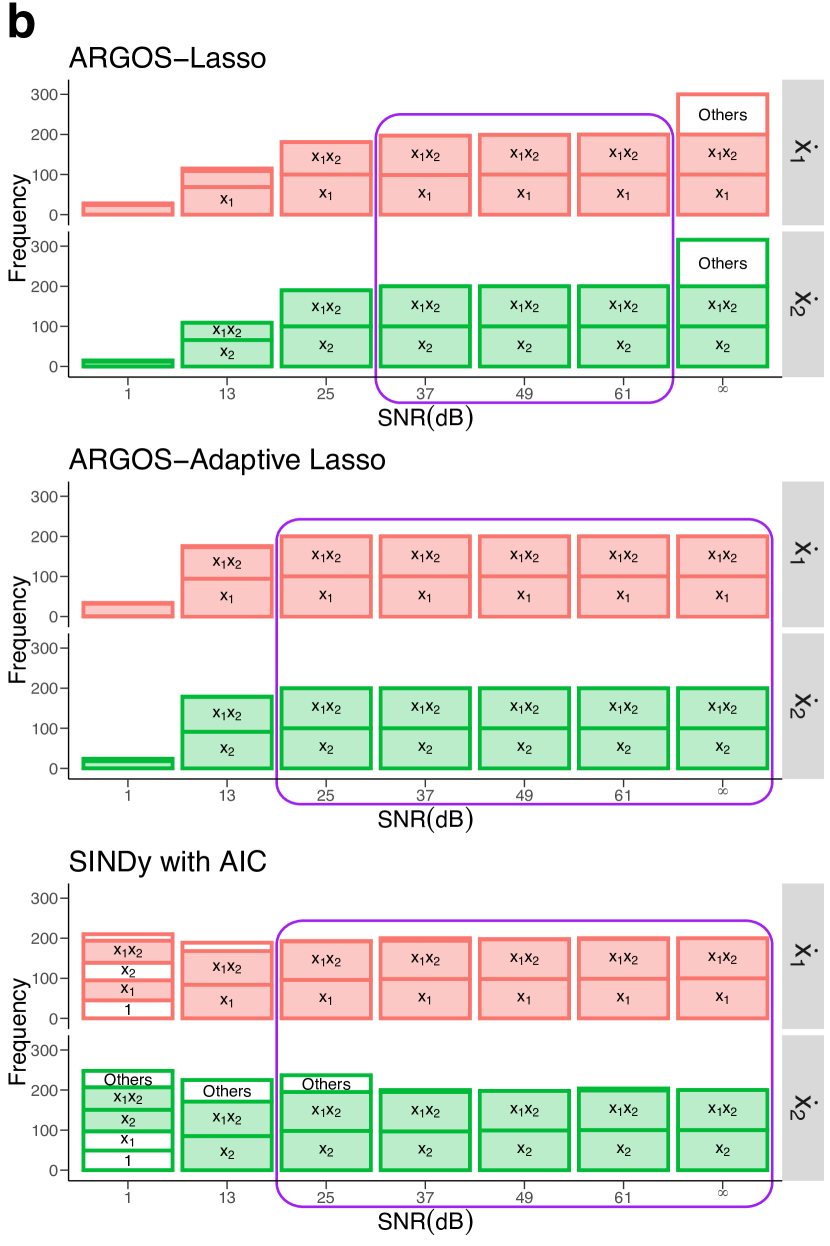
Figure S4: Frequency of identified variables for the Lotka-Volterra system across algorithms. Colors correspond to each governing equation; filled boxes indicate correctly identified variables, while white boxes denote erroneous terms. Panels show the frequency of identified variables for data sets with (a) increasing $n$ (SNR = 49 dB), and (b) SNR ($n=5000$). Purple-bordered regions demarcate model discovery above 80%.

Figure S4 illustrates that, as $n$ and SNR increased, we most consistently identified the true governing terms of the equations using the adaptive lasso within our framework. In contrast, SINDy with AIC tended to discover numerous erroneous terms when data contained fewer than 3000 observations and low SNR.

Rossler system

We examined the Rossler system, a three-dimensional chaotic system represented as

$$\dot{x}_{1} =-x_{2}-x_{3},$$ (S5)

$$\dot{x}_{2} =x_{1}+ax_{2},$$

$$\dot{x}_{3} =b+x_{3}(x_{1}-c),$$

where $a=0.2$, $b=0.2$, and $c=5.7$ [57]. For $x_{1}(t)$, $x_{2}(t)$, and $x_{3}(t)$, we generated a random uniform distribution containing 100 values between $[-10,10]$, $[-10,10]$, and $[0,20]$.

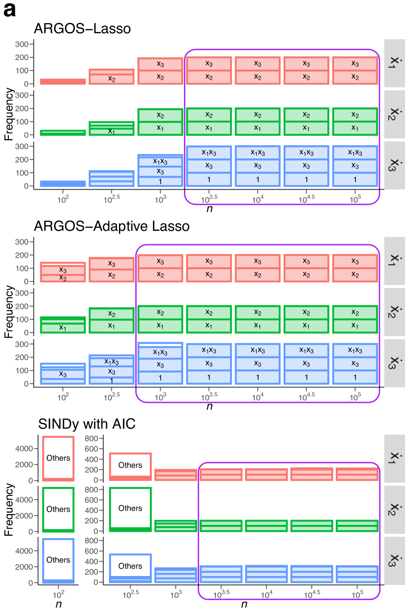
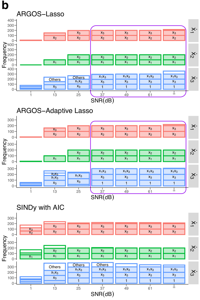
Figure S5: Frequency of identified variables for the Rossler system across algorithms. Colors correspond to each governing equation; filled boxes indicate correctly identified variables, while white boxes denote erroneous terms. Panels show the frequency of identified variables for data sets with (a) increasing $n$ (SNR = 49 dB), and (b) SNR ($n=5000$). Purple-bordered regions demarcate model discovery above 80%.

Figure S5 demonstrates the effectiveness of our approach in accurately representing the Rossler system, provided that sufficient data is available. Here, our method consistently identified the underlying dynamics while SINDy with AIC failed to surpass 80% success for any SNR value, emphasizing the limitations of the sequential thresholding procedure.

Lorenz system

We examined the Lorenz chaotic system, a low-dimensional nonlinear structure originally a simple model for atmospheric convection. The Lorenz systems are modeled using the following equations:

$$\dot{x}_{1} =\sigma(x_{2}-x_{1}),$$ (S6)

$$\dot{x}_{2} =x_{1}(\rho-x_{3})-x_{2},$$

$$\dot{x}_{3} =x_{1}x_{2}-\zeta x_{3},$$

with the values of the original parameters $\sigma=10$, $\rho=28$, and $\zeta=8/3$ [27]. For $x_{1}(t)$, $x_{2}(t)$, and $x_{3}(t)$, we developed a random uniform distribution containing 100 values between $[-15,15]$, $[-15,15]$, and $[10,40]$. The Results section provides more detail regarding each method’s performance in discovering the Lorenz system.

S4 Second-order nonlinear systems

Van der Pol oscillator

We examined the Van der Pol oscillator, introduced in 1922 as a nonlinear circuit model with a triode tube, represented as

$$\dot{x}_{1} =x_{2},$$ (S7)

$$\dot{x}_{2} =\mu(1-x_{1}^{2})x_{2}-x_{1},$$

where $\mu=1.2$ controls the nonlinear damping level of the system [36]. For $x_{1}(t)$ and $x_{2}(t)$, we developed a random uniform distribution containing 100 values between $[-4,4]$.

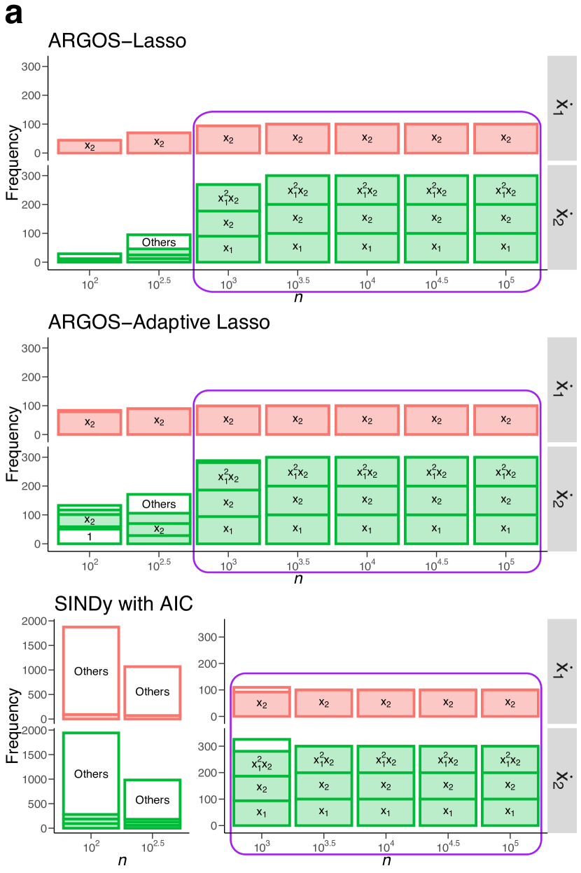
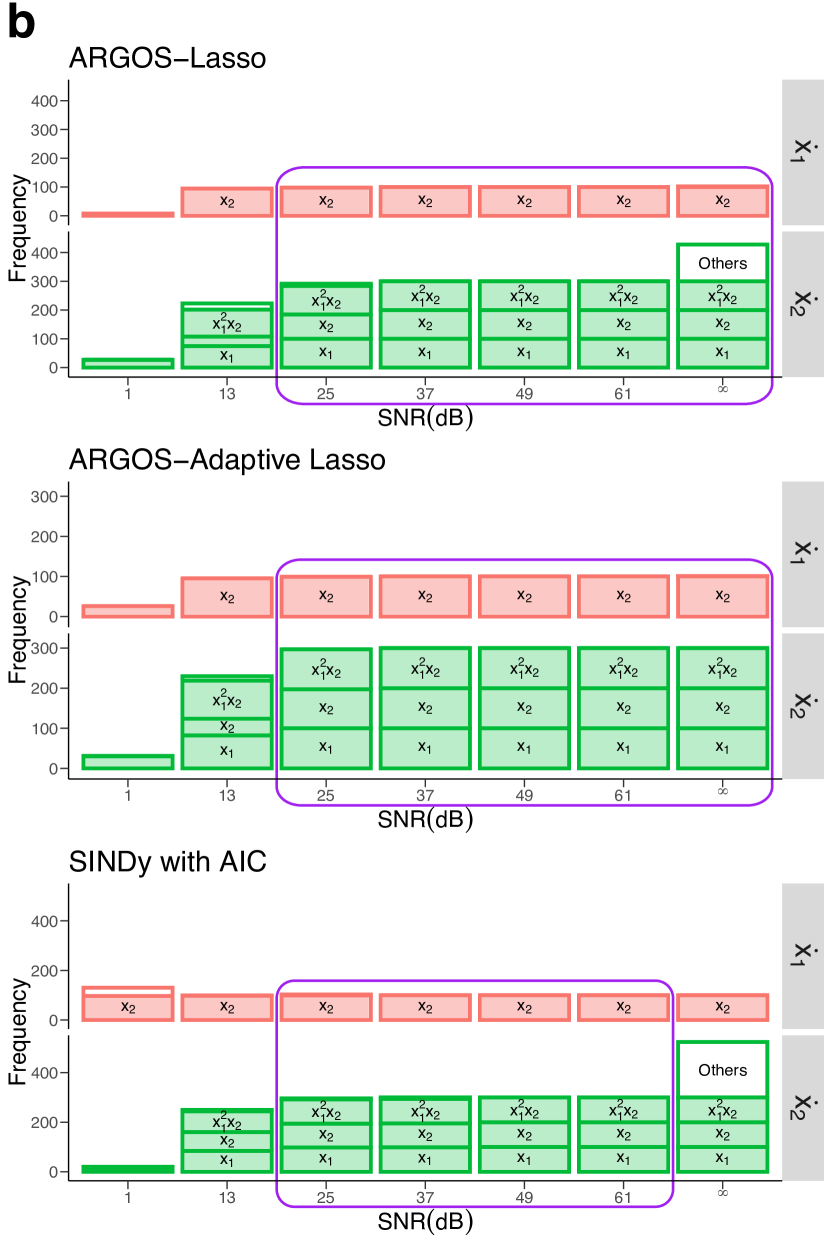
Figure S6: Frequency of identified variables for the Van der Pol oscillator across algorithms. Colors correspond to each governing equation; filled boxes indicate correctly identified variables, while white boxes denote erroneous terms. Panels show the frequency of identified variables for data sets with (a) increasing $n$ (SNR = 49 dB), and (b) SNR ($n=5000$). Purple-bordered regions demarcate model discovery above 80%.

Figure S6 further illustrates the tendencies of each algorithm when faced with a limited number of observations and low SNR. Under these conditions, our method developed overly sparse models, while SINDy with AIC produced dense models that did not accurately represent the Van der Pol oscillator. However, as $n$ and SNR increased, our approach demonstrated a marked improvement in accurately discovering the underlying equations of the oscillator.

Duffing oscillator

We examined the Duffing oscillator as an alternative cubic nonlinear system that can represent chaos. The Duffing oscillator models a spring-damper-mass system that contains a spring with a restoring force of $f(\zeta)=-\kappa\zeta-\epsilon\zeta^{3}$, where $\epsilon>0$ represents a hard spring [36]. However, when $\epsilon<0$, it represents a soft spring and is given by

$$\ddot{\zeta}_{1}+\gamma\dot{\zeta}+(\kappa+\epsilon\zeta^{2})\zeta=0.$$ (S8)

We converted $x=\zeta$ and $y=\dot{\zeta}$ and transformed Eq. (S8) to

$$\dot{x}_{1} =x_{2},$$ (S9)

$$\dot{x}_{2} =-\gamma x_{2}-\kappa x_{1}-\epsilon x_{1}^{3}.$$

Here, we used parameter values for which the Duffing oscillator does not represent chaotic behavior: $\kappa=1$, $\gamma=1$, and $\epsilon=5$  [36]. For $x_{1}(t)$ and $x_{2}(t)$, we developed a random uniform distribution containing 100 values between $[-2,2]$, $[-6,6]$.

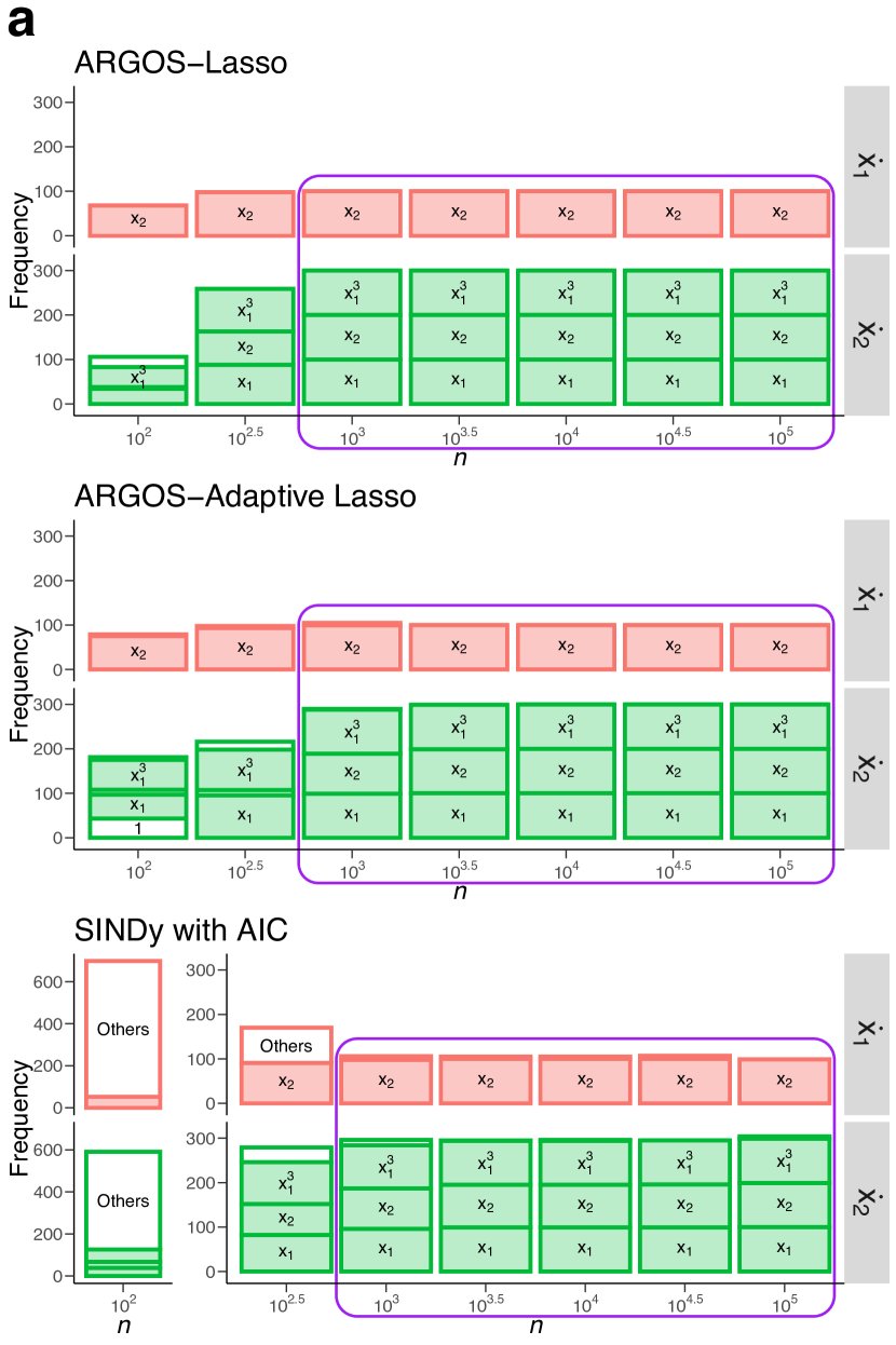
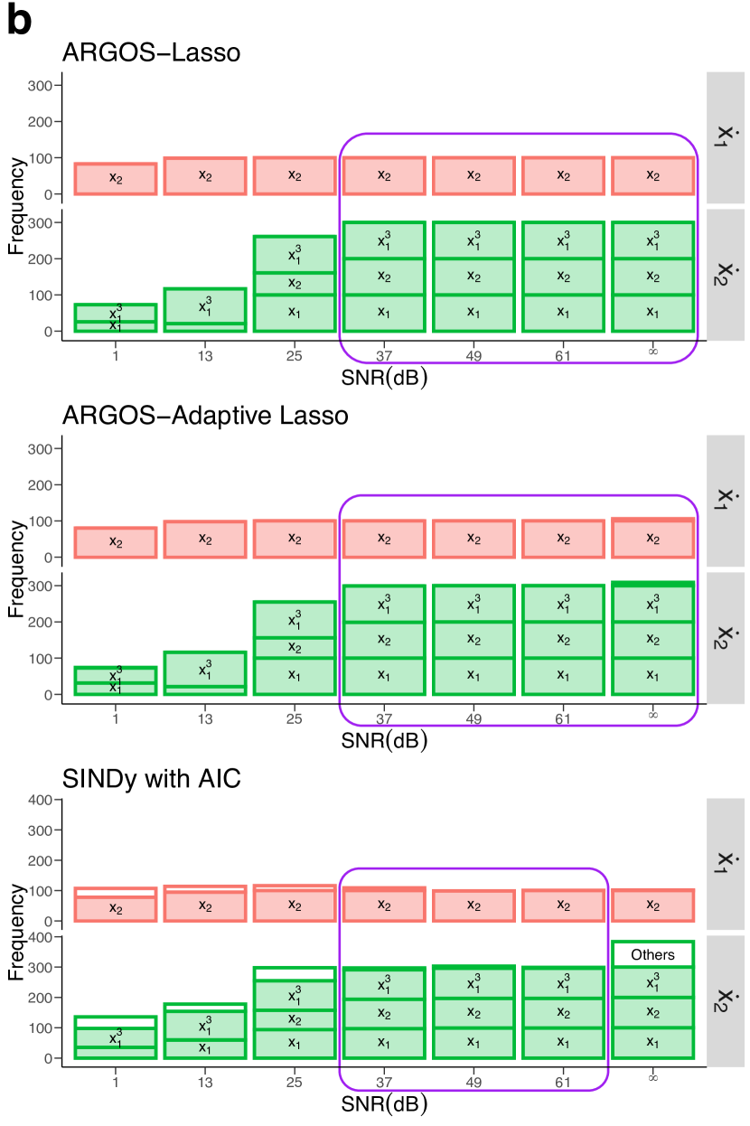
Figure S7: Frequency of identified variables for the Duffing oscillator across algorithms. Colors correspond to each governing equation; filled boxes indicate correctly identified variables, while white boxes denote erroneous terms. Panels show the frequency of identified variables for data sets with (a) increasing $n$ (SNR = 49 dB), and (b) SNR ($n=5000$). Purple-bordered regions demarcate model discovery above 80%.

Figure S7 shows that our method consistently represented the Duffing oscillator with high accuracy as $n$ and SNR increased. In this example, with less than 1000 observations and low SNR, our approach developed overly sparse models that inadequately captured the dynamics of the system, while SINDy with AIC again developed dense models that misrepresented the dynamics.

S5 Algorithms

Algorithm 1 Automatic Savitzky-Golay Filter

1:$\mathbf{\tilde{X}}\in\mathbb{R}^{n\times m}$, $\ dt$.

2:Savitzky-Golay optimally smoothed $\mathbf{X}$ and $\mathbf{\dot{X}}$.

3:determine lower and upper bounds of (odd) window length $l$: $l_{min}=13$, $l_{max}=\max\left(13,\ \min\left(n-\left(n-1\right)\bmod 2,101\right)\ \right)$;

4:build $L=(l_{min},\dots,l_{max})$;

5:$\triangleright$ $v=$ degree of derivative

6:for $j=1,\dots,m$ do $l^{\ast}=\operatorname*{\arg\min}_{L}\|SG(\mathbf{\tilde{x}}_{j},o=4,l=L,v=0,dt)-\mathbf{\tilde{x}}_{j}\|^{2}_{2}$, $\mathbf{x}_{j}=SG(\mathbf{\tilde{x}}_{j},o=4,l=l^{\ast},v=0,dt)$, $\mathbf{\dot{x}}_{j}=SG(\mathbf{\tilde{x}}_{j},o=4,l=l^{\ast},v=1,dt)$;

7:end for

8:consolidate $\mathbf{X},\mathbf{\dot{X}}\in\mathbb{R}^{n\times m}$ with each $\mathbf{x}_{j}$ and $\mathbf{\dot{x}}_{j}$, respectively.

Algorithm 2 Automatic Regression for Governing Equations (ARGOS)

1:$\mathbf{X}\in\mathbb{R}^{n\times m}$, $\mathbf{\dot{x}}_{j}\in\mathbb{R}^{n}$, $d$, $\alpha=0.05$.

2:$\triangleright$ STEP ONE: Initial design matrix

3:$p^{(0)}=\binom{m+d}{d}$;

4:create $\mathbf{\Theta}^{(0)}(\mathbf{X})\in\mathbb{R}^{n\times p^{(0)}}$ with basis functions up to order $d$ of the columns of $\mathbf{X}$;

5:$\triangleright$ STEP TWO: Trim design matrix

6:$\triangleright$ Variable selection with the lasso or adaptive lasso

7:$\triangleright$ $\lambda^{\ast}$ : Optimal $\lambda$ from 10-fold cross-validation

8:$\triangleright$ lasso: $w=1$

9:$\triangleright$ adaptive lasso: $w=$ ridge regression coefficients

10:$\begin{aligned} \hat{\beta}^{(0)}=\operatorname*{\arg\min}_{\beta}\left\|\mathbf{\dot{x}}_{j}-\mathbf{\Theta}^{(0)}(\mathbf{X})\beta\right\|_{2}^{2}+\lambda^{\ast}\sum_{k=1}^{p^{(0)}}w_{k}|\beta_{k}|\end{aligned}$;

11:extract $\mathbf{\Theta}^{(1)}(\mathbf{X})$ to contain columns of $\mathbf{\Theta}^{(0)}(\mathbf{X})$ up to the largest order $d^{(1)}$ of the selected variables in $\hat{\beta}^{(0)}$;

12:$\triangleright$ STEP THREE: Final point estimates

13:$\triangleright$ Repeat sparse regression algorithm from STEP TWO

14:$p^{(1)}=\binom{m+d^{(1)}}{d^{(1)}}$;

15:$\begin{aligned} \hat{\beta}^{(1)}&=\operatorname*{\arg\min}_{\beta}\left\|\mathbf{\dot{x}}_{j}-\mathbf{\Theta}^{(1)}(\mathbf{X})\beta\right\|_{2}^{2}+\lambda^{\ast}\sum_{k=1}^{p^{(1)}}w_{k}|\beta_{k}|;\end{aligned}$

16:$\triangleright$ Apply threshold values

17:$\eta=[10^{-8},10^{-7},\dotsc,10^{1}]$;

18:for $i=1,\dots,\mathbf{card}(\eta)$ do

19:$\triangleright$ Ordinary least squares regression (OLS) estimate after variable selection$\begin{aligned} \hat{\beta}^{\text{OLS}}[i]&=\operatorname*{\arg\min}_{\beta_{\mathcal{K}_{i}}}\left\|\mathbf{\dot{x}}_{j}-\mathbf{\Theta}_{\mathcal{K}_{i}}^{(1)}(\mathbf{X})\beta_{\mathcal{K}_{i}}\right\|_{2}^{2}\ \text{where}\ \mathcal{K}_{i}=\{k:|\hat{\beta}_{k}^{(1)}|\geq\eta_{i}\},\\ \end{aligned}$ $\text{BIC}_{i}=\text{BIC}(\hat{\beta}^{\text{OLS}}[i])$;

20:end for

21:$\hat{\beta}=\left\{\hat{\beta}^{\text{OLS}}[i]\middle|i:\operatorname*{\arg\min}(\text{BIC})\right\};$

22:$\triangleright$ STEP FOUR: Bootstrap estimates for confidence intervals

23:$\triangleright$ $B=2000$ bootstrap samples

24:bootstrap Statements 15 – 21 to approximate confidence interval bounds: $CI_{\text{lo}}=[B\alpha/2]$ and $CI_{\text{up}}=B-CI_{\text{lo}}+1$;

25:construct bootstrap confidence intervals for $\hat{\beta}$: $\begin{aligned} \hat{\beta}_{k}\in\left[\hat{\beta}_{k}^{\text{OLS}\{CI_{\text{lo}}\}},\hat{\beta}_{k}^{\text{OLS}\{CI_{\text{up}}\}}\right]\text{, and }0<\hat{\beta}_{k}^{\text{OLS}\{CI_{\text{lo}}\}}\text{ or }0>\hat{\beta}_{k}^{\text{OLS}\{CI_{\text{up}}\}}\end{aligned}$.

References

- [1] David Ruelle and Floris Takens. On the nature of turbulence. Communications in Mathematical Physics, 20(3):167–192, September 1971.
- [2] Duncan J. Watts and Steven H. Strogatz. Collective dynamics of ‘small-world’ networks. Nature, 393(6684):440–442, June 1998.
- [3] Valery Petrov, Vilmos Gáspár, Jonathan Masere, and Kenneth Showalter. Controlling chaos in the Belousov—Zhabotinsky reaction. Nature, 361(6409):240–243, January 1993.
- [4] Michael C. Mackey and Leon Glass. Oscillation and Chaos in Physiological Control Systems. Science, 197(4300):287–289, July 1977.
- [5] John J. Tyson, Kathy Chen, and Bela Novak. Network dynamics and cell physiology. Nature Reviews Molecular Cell Biology, 2(12):908–916, December 2001.
- [6] Ralf Steuer, Thilo Gross, Joachim Selbig, and Bernd Blasius. Structural kinetic modeling of metabolic networks. Proc. Natl. Acad. Sci. U.S.A., 103(32):11868–11873, August 2006.
- [7] Eric Karsenti. Self-organization in cell biology: A brief history. Nat Rev Mol Cell Biol, 9(3):255–262, March 2008.
- [8] Boris N. Kholodenko, John F. Hancock, and Walter Kolch. Signalling ballet in space and time. Nat Rev Mol Cell Biol, 11(6):414–426, June 2010.
- [9] Philipp M. Altrock, Lin L. Liu, and Franziska Michor. The mathematics of cancer: Integrating quantitative models. Nat Rev Cancer, 15(12):730–745, December 2015.
- [10] Dante R. Chialvo. Emergent complex neural dynamics. Nature Physics, 6(10):744–750, October 2010.
- [11] Emanuel Todorov. Optimality principles in sensorimotor control. Nature Neuroscience, 7(9):907–915, September 2004.
- [12] Michael Breakspear. Dynamic models of large-scale brain activity. Nature Neuroscience, 20(3):340–352, March 2017.
- [13] George Sugihara and Robert M. May. Nonlinear forecasting as a way of distinguishing chaos from measurement error in time series. Nature, 344(6268):734–741, April 1990.
- [14] David J. D. Earn, Pejman Rohani, Benjamin M. Bolker, and Bryan T. Grenfell. A Simple Model for Complex Dynamical Transitions in Epidemics. Science, 287(5453):667–670, January 2000.
- [15] George Sugihara, Robert May, Hao Ye, Chih-hao Hsieh, Ethan Deyle, Michael Fogarty, and Stephan Munch. Detecting causality in complex ecosystems. Science, 338(6106):496–500, 2012.
- [16] Simon N. Wood. Statistical inference for noisy nonlinear ecological dynamic systems. Nature, 466(7310):1102–1104, August 2010.
- [17] C. Nicolis and G. Nicolis. Reconstruction of the dynamics of the climatic system from time-series data. Proc. Natl. Acad. Sci. U.S.A., 83(3):536–540, February 1986.
- [18] Will Steffen, Johan Rockström, Katherine Richardson, Timothy M. Lenton, Carl Folke, Diana Liverman, Colin P. Summerhayes, Anthony D. Barnosky, Sarah E. Cornell, Michel Crucifix, Jonathan F. Donges, Ingo Fetzer, Steven J. Lade, Marten Scheffer, Ricarda Winkelmann, and Hans Joachim Schellnhuber. Trajectories of the Earth System in the Anthropocene. Proc. Natl. Acad. Sci. U.S.A., 115(33):8252–8259, August 2018.
- [19] David Waltz and Bruce G. Buchanan. Automating Science. Science, 324(5923):43–44, April 2009.
- [20] Michael D Schmidt, Ravishankar R Vallabhajosyula, Jerry W Jenkins, Jonathan E Hood, Abhishek S Soni, John P Wikswo, and Hod Lipson. Automated refinement and inference of analytical models for metabolic networks. Phys. Biol., 8(5):055011, October 2011.
- [21] James P Crutchfield and Bruce McNamara. Equations of Motion from a Data Series. Complex Systems, 1:417–452, 1987.
- [22] Albert Tarantola. Inverse Problem Theory and Methods for Model Parameter Estimation. Society for Industrial and Applied Mathematics, January 2005.
- [23] X. Hong, R.J. Mitchell, S. Chen, C.J. Harris, K. Li, and G.W. Irwin. Model selection approaches for non-linear system identification: A review. International Journal of Systems Science, 39(10):925–946, October 2008.
- [24] Michael Schmidt and Hod Lipson. Distilling free-form natural laws from experimental data. Science, 324(5923):81–85, April 2009.
- [25] H. Schaeffer, R. Caflisch, C. D. Hauck, and S. Osher. Sparse dynamics for partial differential equations. Proceedings of the National Academy of Sciences, 110(17):6634–6639, April 2013.
- [26] Bryan Daniels and Ilya Nemenman. Automated adaptive inference of phenomenological dynamical models. Nat Commun, 6(1):8133, November 2015.
- [27] Steven L. Brunton, Joshua L. Proctor, and J. Nathan Kutz. Discovering governing equations from data by sparse identification of nonlinear dynamical systems. Proc Natl Acad Sci USA, 113(15):3932–3937, April 2016.
- [28] Maziar Raissi, Paris Perdikaris, and George Em Karniadakis. Machine learning of linear differential equations using Gaussian processes. Journal of Computational Physics, 348:683–693, November 2017.
- [29] Hayden Schaeffer. Learning partial differential equations via data discovery and sparse optimization. Proc. R. Soc. A., 473(2197):20160446, January 2017.
- [30] Hayden Schaeffer, Giang Tran, and Rachel Ward. Extracting sparse high-dimensional dynamics from limited data. SIAM J. Appl. Math., 78(6):3279–3295, January 2018.
- [31] Maziar Raissi and George Em Karniadakis. Hidden physics models: Machine learning of nonlinear partial differential equations. Journal of Computational Physics, 357:125–141, March 2018.
- [32] Bethany Lusch, J. Nathan Kutz, and Steven L. Brunton. Deep learning for universal linear embeddings of nonlinear dynamics. Nat Commun, 9:4950, December 2018.
- [33] Sheng Zhang and Guang Lin. Robust data-driven discovery of governing physical laws with error bars. Proc. R. Soc. A., 474(2217):20180305, September 2018.
- [34] Roger Guimerà, Ignasi Reichardt, Antoni Aguilar-Mogas, Francesco A. Massucci, Manuel Miranda, Jordi Pallarès, and Marta Sales-Pardo. A Bayesian machine scientist to aid in the solution of challenging scientific problems. Sci. Adv., 6(5):107077, January 2020.
- [35] Silviu-Marian Udrescu and Max Tegmark. AI Feynman: A physics-inspired method for symbolic regression. Sci. Adv., 6(16):eaay2631, April 2020.
- [36] Alexandre Cortiella, Kwang-Chun Park, and Alireza Doostan. Sparse identification of nonlinear dynamical systems via reweighted $\ell_1$-regularized least squares. Computer Methods in Applied Mechanics and Engineering, 376:113620, April 2021.
- [37] Jared L. Callaham, James V. Koch, Bingni W. Brunton, J. Nathan Kutz, and Steven L. Brunton. Learning dominant physical processes with data-driven balance models. Nat Commun, 12:1016, December 2021.
- [38] Ye Yuan, Xiuchuan Tang, Wei Zhou, Wei Pan, Xiuting Li, Hai-Tao Zhang, Han Ding, and Jorge Goncalves. Data driven discovery of cyber physical systems. Nat Commun, 10(1):4894, October 2019.
- [39] N. M. Mangan, J. N. Kutz, S. L. Brunton, and J. L. Proctor. Model selection for dynamical systems via sparse regression and information criteria. Proc. R. Soc. A., 473(2204):20170009, August 2017.
- [40] John Guckenheimer and Philip Holmes. Nonlinear Oscillations, Dynamical Systems, and Bifurcations of Vector Fields, volume 42. Springer Science \& Business Media, New York, NY, 2013.
- [41] Abraham Savitzky and M. J. E. Golay. Smoothing and differentiation of data by simplified least squares procedures. Anal. Chem., 36(8):1627–1639, July 1964.
- [42] William H. Press, Saul A. Teukolsky, William T. Vetterling, and Brian P. Flannery. Numerical Recipes: The Art of Scientific Computing. Cambridge University Press, New York, third edition, 2007.
- [43] R. Tibshirani. Regression shrinkage and selection via the Lasso. Journal of the Royal Statistical Society. Series B (Methodological), 58:267–288, 1996.
- [44] Hui Zou. The Adaptive Lasso and its oracle properties. Journal of the American Statistical Association, 101(476):1418–1429, December 2006.
- [45] Gideon Schwarz. Estimating the dimension of a model. The Annals of Statistics, 6(2):461–464, March 1978.
- [46] Bradley Efron and Robert Tibshirani. An Introduction to the Bootstrap. Number 57 in Monographs on Statistics and Applied Probability. Chapman & Hall, New York, 1993.
- [47] Robert Tibshirani, Jerome H. Friedman, and Trevor Hastie. The Elements of Statistical Learning. Springer, New York, 2009.
- [48] Arthur E. Hoerl and Robert W. Kennard. Ridge regression: Biased estimation for nonorthogonal problems. Technometrics, 12(1):55–67, February 1970.
- [49] Trevor Hastie, Robert Tibshirani, and Martin Wainwright. Statistical Learning with Sparsity (Old Version with Highlights). CRC Press, New York, 2015.
- [50] Jerome Friedman, Trevor Hastie, and Robert Tibshirani. Regularization paths for generalized linear models via Coordinate Descent. J. Stat. Soft., 33(1):1–22, 2010.
- [51] Peter Bühlmann and Sara van de Geer. Statistics for High-Dimensional Data. Springer Series in Statistics. Springer Berlin Heidelberg, Berlin, Heidelberg, 2011.
- [52] Hui Zou, Trevor Hastie, and Robert Tibshirani. On the “degrees of freedom” of the lasso. Ann. Statist., 35(5), October 2007.
- [53] Abdelhak M Zoubir and D Robert Iskander. Bootstrap Techniques for Signal Processing. Cambridge University Press, Cambridge, 2004.
- [54] Richard G. Lyons. Understanding Digital Signal Processing. Pearson, Boston, MA, third edition, 2011.
- [55] Alfred J. Lotka. Contribution to the Theory of Periodic Reactions. J. Phys. Chem., 14(3):271–274, March 1910.
- [56] Gustavo T. Naozuka, Heber L. Rocha, Renato S. Silva, and Regina C. Almeida. SINDy-SA framework: Enhancing nonlinear system identification with sensitivity analysis. Nonlinear Dyn, 110(3):2589–2609, November 2022.
- [57] Giang Tran and Rachel Ward. Exact Recovery of Chaotic Systems from Highly Corrupted Data. Multiscale Model. Simul., 15(3):1108–1129, January 2017.