Convergence of Message Passing Graph Neural Networks with Generic Aggregation On Large Random Graphs

Abstract.

We study the convergence of message passing graph neural networks on random graph models to their continuous counterpart as the number of nodes tends to infinity. Until now, this convergence was only known for architectures with aggregation functions in the form of normalized means, or, equivalently, of an application of classical operators like the adjacency matrix or the graph Laplacian. We extend such results to a large class of aggregation functions, that encompasses all classically used message passing graph neural networks, such as attention-based message passing, max convolutional message passing or (degree-normalized) convolutional message passing. Under mild assumptions, we give non-asymptotic bounds with high probability to quantify this convergence. Our main result is based on the McDiarmid inequality. Interestingly, this result does not apply to the case where the aggregation is a coordinate-wise maximum. We treat this case separately and obtain a different convergence rate.

1Introduction

Graph Neural Networks (GNNs) [SGT⁺09, GMS05] are deep learning architectures largely inspired by Convolutional Neural Networks, that aim to extend convolutional methods to signals on graphs. Indeed, in many domains the measured data live on a graph structure: examples for which GNNs have achieved state-of-the-art performance include molecules, proteins and node clustering [GSR⁺17, CLB19, FBSBH17]. Nevertheless, it has been observed that GNNs have limitations, both in practice [WSZ⁺19, HFZ⁺20] and in their theoretical understanding. Hence, the design of more reliable and powerful architectures is a current active and fast evolving area of research.

From a theoretical perspective, a large part of the literature has focused on the expressive power of GNNs, i.e. what class of functions can GNNs approximate. This notion is fundamental in classical Deep Learning and is related to the so-called Universal Approximation Theorem [KH91, Cyb89]. Studying the expressive power of GNNs is however more involved, as they are by definition designed to be invariant or equivariant to the relabelling of nodes in a graph (see Sec. 3). Hence, in [XHLJ19] the authors relate their expressivity to the graph isomorphism problem, that is, deciding if two graphs are permutation of one another, a long-standing combinatorial problem in graph theory. The main avenue to analyze the expressive power of GNNs compares their performances to the traditional Weisfeiler-Lehman algorithm (WL) [WL68], which process is very similar to the message-passing paradigm at the core of GNNs. Hence, by construction, basic GNNs are at most as powerful as WL [XHLJ19]. From this point, a lot of effort has been made on designing innovative GNN architectures to outperform the classical WL [MFSL19, MBHSL19, KP19, VLF20, PW22, MRM20].

Nevertheless, while this combinatorial approach is worth considering for reasonably small graphs, its relevance in the context of large graphs is somewhat limited. Two real large graphs may share similar patterns, but will never be isomorphic, one main simple reason being that they most likely do not even share the same number of nodes. Large graphs are better described by some global properties such as edge density or number of communities. To that extent, the privileged mathematical tools are random graph models [Cra18, GZF⁺10]. A generic family of models of interest to study GNNs on large graphs is the class of Latent Position Models [KBV20, KBV21, RCR20, RCR21a, LHB⁺21, MLLK22]. Such random graphs first sample node latent variables randomly from a probability space $(\mathcal{X},P)$, and then decides the adjacency between two nodes via the sampling of a connectivity kernel $W:\mathcal{X}^{2}\to[0,1]$ between their associated latent variables. This encompasses models like stochastic block models [LR15] (SBM) or graphon models [Lov12], depending on how exactly we define the edge appearance procedure.

The key idea in studying GNNs on large random graphs is to embed the discrete problem into a continuous setting for which we expect to understand their properties with more ease [KBV20, KBV21, RCR20, LHB⁺21]. To achieve this, we match the GNN on a random graph to a “continuous” counterpart, referred to as a continuous-GNN (cGNN) [KBV20, RCR21a]. While the discrete GNN propagates a signal over the nodes of the graph, the cGNN propagates a mapping over the latent space $\mathcal{X}$. Such a map can be interpreted as a signal over the graph where the “continuum” of nodes would be all the points of $\mathcal{X}$. Then, as the random graph grows large, the GNN must behave similarly to its cGNN counterpart. To justify this, it is necessary to describe the cGNN as a limit of GNNs on random graphs and to ensure that the GNN converges to the cGNN as the number of nodes increases [KBV20, MLLK22]. This convergence problem is precisely the focus of the present work.

The duality of the convolutional product has led to two ways of defining GNNs. On the one hand, convolution as a pointwise product of frequencies in the Fourier domain has justified the design of so-called Spectral Graph Neural Networks [DBV16] (SGNNs), in which one introduces a graph Fourier transform through a chosen graph shift operator [TGB18] to legitimate the use of polynomial filters. On the other hand, the spatial interpretation sees the convolution as local aggregations of neighborhood information, leading to Message Passing Neural Networks (MPGNNs) [GSR⁺17, KW17]. The message passing paradigm consists of iteratively updating each node via the aggregation of messages from each of its neighbors. This framework is often favored due to its inherent flexibility: messages and aggregation functions are unconstrained as long as they stay invariant to node reordering, i.e., as long as they match on isomorphic graphs. Besides, SGNNs layers are mostly made of polynomials of graph shift operators which are a form of message passing, defined by a choice of graph shift operator and a polynomial degree. As such, SGNNs can be seen as a subcase of the more versatile message-passing framework.

Contributions.

In this paper, we study the convergence toward a continuous counterpart of MPGNNs with a generic aggregation function, whereas previous work [KBV20, KBV21, RCR21b, MLLK22] are restricted to SGNNs or MPGNNs with specific aggregations. We use a simple version of the Latent Space Model where random graphs are totally connected and weighted accordingly the sampling of the kernel $W$ at the latent positions. Our main result, Theorem 5.7, states that for MPGNNs having a Lipschitz-type regularity, the discrete network on a large random graph is close to its continuous counterpart with high probability. We quantify this convergence via a non asymptotic bound based on the McDiarmid concentration inequality for multivariate functions of independent random variables. A special treatment is given to the case where the aggregation is a coordinate-wise maximum [FL19]. For that particular case, Theorem 5.7 does not hold. Thus, we provide another proof of convergence based on a specific concentration inequality, in Theorem 5.12. This results in a significantly different theoretical convergence rate.

Related work.

The closest related works to ours are the results from Keriven et al. [KBV20, KBV21], where they establish convergence of SGNN on Latent Position random graphs. We also mention Maskey et al. [MLLK22] that studies a particular case of MPGNN on large random graphs, where the aggregation is defined to be a mean normalized by the degree of the node. The present paper can be considered as a direct extension of both these works in the setting of MPGNNs with generic aggregation.

Further, the concept of limit of a SGNN on large random graphs has shown fruitful to tackle several problems. For instance, multiple works from different authors, among which [KBV20, MLK23a, LHB⁺21, RCR21b, CRR23], have focus on stability to deformation or transferability. The idea being that, since the same GNN can be applied to any graph, no matter its size or structure, we expect the outputs to be close on similar graphs, which is particularly relevant for large random graphs drawn from the same (or almost same) model. Concerning the expressive power on large graphs, Keriven et al. exploit their convergence theorems from [KBV20, KBV21] to propose a description of the function space that SGNNs on random graphs can approximate in [KV23] and derive certain properties of universality. About other topics related to the learning procedure such as generalization as well as oversmoothing, the authors in [MLLK22] derive a generalization bound that gets tighter for large graphs, while the results described in [Ker22] make use of Latent Position random graphs to search a threshold between beneficial finite smoothing and oversmoothing.

Beyond random graphs, large (dense) graphs can be described through the theory of graphons [Lov12]. Indeed, with the so-called cut metric, the space of all graphs can be completed to obtain a compact space: the space of graphons, in which any graphon is a limit of discrete graphs. Several works aim to characterize the convergence of GNNs on large graphs with these mathematical tools. In [RCR20, MLK23b], the authors define limits of graph polynomial filters of SGNNs designed from graph shift operators as integral operators w.r.t. the underlying graphon, and make use of the theory of self adjoint operators and Hilbert spaces to study them. More recently, authors in [BLH⁺23] consider a continuous version of the WL test via graphon estimation to study expressive power and the paper [Lev23] is devoted to extend the concept of sampling graphs from graphon to sampling graph signals from graphon signals.

Outline.

In Section 2, we give some basic definitions. In Section 3 we define MPGNNs with a generic aggregation function, that is, any function on sets used to gather and combine neighborhood information in the message-passing paradigm. In Section 4 we introduce continuous-MPGNNs (cMPGNNs) which are the counterpart of discrete MPGNNs that propagate a function over a compact probability space, alongside a connectivity kernel. As a discrete MPGNN must be coherent with graph isomorphism, we give mild conditions under which the cMPGNN is coherent with respect to some notion of probability space isomorphism. In Section 5, we focus on MPGNNs when applied on random graphs and describe what class of cMPGNN would be their natural limit. Our main result is Theorem 5.7: it provides necessary conditions under which the discrete network converges to its continuous counterpart. We make use of the McDiarmid concentration inequality to derive a non asymptotic bound with high probability of the deviation between the outputs of the MPGNN and its limit cMPGNN. Overall, we conclude that a sufficient condition of convergence is for the aggregation to have sharp bounded differences. All along the paper, we illustrate our concepts on classical GNN examples from the basic Graph Convolutional Network to the more sophisticated Graph Attentional Network [VCC⁺17]. We give a particular treatment to the case of the maximum aggregation. Indeed, its behavior turns out to be significantly different than the other examples and do not fit into the class of MPGNNs having sharp bounded differences. Nevertheless, in Theorem 5.12 we make use of other specific concentration bounds to prove another non asymptotic bound between max MPGNN and its limit cMPGNN, with a significantly different convergence rate.

2Notations and Definitions

We start by introducing the notations that will hold throughout the paper. The letter $d$ (and its derived $d_{0},d^{(0)},\ldots$) will represent the dimension of a real vector space, the letter $n$ will denote the number of nodes in a graph, and $L$ will refer to the total number of layers in a deep architecture. Whenever we need to index something relatively to vertices of a graph, we use a subscript indexation (e.g., $z_{i}$) and in the case of layers, we employ a superscript (e.g., $z^{(l)}$).

We fix a positive integer $d$ and $(\mathbb{R}^{d},\|\cdot\|_{\infty},\mathbb{B}(\mathbb{R}^{d}))$ the $d$-dimensional real vector space endowed with the infinite norm $\|x\|_{\infty}=\max_{i}|x_{i}|$ as well as its Borel sigma algebra. Except when specified differently, any topological concept, such as balls, continuity, etc., will be considered relatively to the norm $\|\cdot\|_{\infty}$. All along this paper, $\mathcal{X}$ is a compact subset of $\mathbb{R}^{d}$ and $\mathcal{B}(\mathcal{X})$ its Borel sigma algebra defined as the sigma algebra generated by the $U\cap\mathcal{X}$, for the open sets $U$ of $\mathbb{R}^{d}$.

The group of permutations of $\{1,\dots,n\}$ is denoted as $S_{n}$. If $x=(x_{1},\dots,x_{n})$ is an $n$-tuple and $\sigma$ an element of $S_{n}$, we define the $n$-tuple $\sigma\cdot x$ as $\sigma\cdot x=(x_{\sigma^{-1}(1)},\dots,x_{\sigma^{-1}(n)})$.

The set of bijections $\phi$ of $\mathcal{X}$ such that both $\phi$ and $\phi^{-1}$ are measurable is a group for the composition of functions. We call it the group of automorphisms of $\mathcal{X}$ and denote it as $\operatorname*{Aut}(\mathcal{X})$. We denote as $\mathcal{P}(\mathcal{X})$ the set of probability measures on $(\mathcal{X},\mathcal{B}(\mathcal{X}))$. For a measure $P\in\mathcal{P}(\mathcal{X})$ and a bijection $\phi\in\operatorname*{Aut}(\mathcal{X})$, the push forward measure of $P$ through $\phi$ is defined as $\phi_{\#}P(A)=P(\phi^{-1}(A))$ for all $A$ in $\mathcal{B}(\mathcal{X}).$ Since this makes the group $\operatorname*{Aut}(\mathcal{X})$ acting on the set of probability measures on $\mathcal{X}$, we also use the notation $\phi\cdot P=\phi_{\#}P$, which is standard for a (left) group action. For the same reason, we shall use the notation $\phi\cdot f=f\circ\phi^{-1}$ and $\phi\cdot W=W(\phi^{-1}(\cdot),\phi^{-1}(\cdot))$ whenever $f$ is a measurable function on $\mathcal{X}$ and $W$ is a bivariate measurable function on $\mathcal{X}\times\mathcal{X}$.

For $P\in\mathcal{P}(X)$, the space $L^{\infty}_{P}(\mathcal{X},\mathbb{R}^{p})$ is the space of essentially bounded (equivalence classes of) maps from $\mathcal{X}$ to $\mathbb{R}^{p}$ endowed with the norm $\|f\|_{P,\infty}=\mathop{\mathrm{ess\,sup}}\limits_{\scriptstyle P,\\ \scriptstyle x\in\mathcal{X}}\|f(x)\|_{\infty}$. When there is no ambiguity on $P$, the norm $\|\cdot\|_{P,\infty}$ is noted $\|\cdot\|_{\infty}$. The space $\mathcal{C}(\mathcal{X},\mathbb{R}^{p})$ is made of the continuous functions from $\mathcal{X}$ to $\mathbb{R}^{p}$. Since $\mathcal{X}$ is compact, any continuous map is bounded thus essentially bounded, which makes $\mathcal{C}(\mathcal{X},\mathbb{R}^{p})$ a subspace of $L^{\infty}_{P}(\mathcal{X},\mathbb{R}^{p})$.

Sets are represented between braces $\{\cdot\}$, whereas multisets, that is, sets in which an element is allowed to appear twice or more, are represented by double braces $\{\!\!\{\cdot\}\!\!\}$. If $m$ and $m^{\prime}$ are two multisets of same size, say $n$, containing elements from a metric space $(\mathcal{E},\delta)$, we define their distance by:

(2.1) $$\delta(m,m^{\prime})=\min_{\sigma\in S_{n}}\max_{x_{i}\in m,x_{i}^{\prime}\in m^{\prime}}\delta(x_{i},x_{\sigma(i)}^{\prime}).$$

We define the sampling operator the following way. If $f:\mathcal{E}_{0}\to\mathcal{E}_{1}$ and $X=(x_{1},\dots,x_{n})\in\mathcal{E}_{0}^{n}$:

(2.2) $$S_{X}f=(f(x_{i}),\dots,f(x_{n}))\in\mathcal{E}_{1}^{n}.$$

2.1Graph-related definitions

In this subsection, we introduce the concepts of discrete graph, graph signal and graph isomorphism.

Graph.

A non oriented weighted graph $G$ with $n$ vertices is defined by a triplet $(V,E,w)$, where $V=\{v_{1},\dots,v_{n}\}$ is a finite set called the set of vertices (or nodes) and $E$ is the set of edges. The set of neighbors of a vertex $v_{i}$ in $G$ is referred to as $\mathcal{N}_{G}(v_{i})$ or simply $\mathcal{N}(v_{i})$ when the underlying graph is clear from context. The weight function $w$ assigns a nonnegative number to each edge. It is often represented by a symmetric function $w:V^{2}\to\mathbb{R}^{+}$ and the abbreviation $w_{i,j}$ is used to denote the weight $w(v_{i},v_{j})=w(v_{j},v_{i})$ where $\{v_{i},v_{j}\}\in E$. In this paper, “graph” will always mean “undirected and weighted graph”. The set of graphs defined on the vertex set $V$ is denoted as $\mathcal{G}(V)$.

Graph signal.

Given a graph $G\in\mathcal{G}(V)$, where $|V|=n$, a signal on $G$ is a map from the set of vertices $V$ to $\mathbb{R}^{d}$ that assigns a $d$-dimensional vector $z_{i}$ to each vertex $v_{i}$. The images from all vertices are stacked into a matrix $Z$ of size $n\times d$. Abusing notations, we may not distinguish between the map and its image $Z$, the latter being also named the signal.

Graph isomorphism.

Two graphs $G_{1}=(V_{1},E_{1},w_{1})$ and $G_{2}=(V_{2},E_{2},w_{2})$ in $\mathcal{G}(V)$, where $|V|=n$, are said to be isomorphic if there is a permutation $\sigma\in S_{n}$ such that $E_{2}=\{\{v_{\sigma^{-1}(i)},v_{\sigma^{-1}(j)}\}|\ \{v_{i},v_{j}\}\in E_{1}\}$ and $w_{2}(v_{i},v_{j})=w_{1}(v_{\sigma^{-1}(i)},v_{\sigma^{-1}(j)})$. In this case we note $G_{2}=\sigma\cdot G_{1}$. Moreover, if $Z$ is a signal on $G_{1}$ and $\sigma\in S_{n}$, $\sigma\cdot Z$ is an isomorphic signal on the graph $\sigma\cdot G_{1}$.

2.2Random Graph Models

Random Graph Model.

A random graph model is a couple $(W,P)$ where $P$ is a Borel probability measure on $\mathcal{X}$ and $W:\mathcal{X}\times\mathcal{X}\mapsto[0,1]$ is a kernel, i.e., a symmetric measurable function. One can interpret $W$ as a totally connected graph on the vertex set $\mathcal{X}$ and whose weight function is $W$.

Random Graph.

We generate random graphs from a random graph model $(W,P)$ as follows. Given a positive integer $n$, we first draw $n$ independent and identically distributed random variables from the distribution $P$, represented by ${X_{1},\dots,X_{n}}$, which form the vertex set of the graph. The random graph is fully connected and has weight function $W$:

$$X_{1},\dots,X_{n}\overset{iid}{\sim}P,\quad w_{i,j}=w_{j,i}=W(X_{i},X_{j}).$$

When convenient, we will use the short notation $X=(X_{1},\dots,X_{n})$ for the tuple of the vertices of a random graph. We call $\mathcal{G}_{n}(W,P)$ the distribution from which random graphs with $n$ nodes are drawn. We bring the reader’s attention to the fact that in the above definition, a random graph is always fully connected but edges may have a weight equal to zero. Another common model [KBV20, LR15] is to add a Bernoulli distribution to the connectivity, similarly to SBM models, in order to model unweighted random graphs, potentially with prescribed expected sparsity. It is not done here for the sake of simplicity: indeed weighted random graphs without Bernoulli edges are routinely used to analyze machine learning algorithms [VBB08, MLLK22], as they essentially model the underlying phenomena of interest in many cases.

Random Graph Model isomorphism.

Two probability measures $P_{1}$ and $P_{2}$ on $\mathcal{X}$ are said isomorphic if there is some $\phi$ in $\operatorname*{Aut}(\mathcal{X})$ such that $P_{2}=\phi_{\#}P_{1}$. Similarly, two random graph models $(W_{1},P_{1})$ and $(W_{2},P_{2})$ on $\mathcal{X}$ are said to be isomorphic if there is a $\phi$ in $\operatorname*{Aut}(\mathcal{X})$ such that $(W_{2},P_{2})=(\phi\cdot W_{1},\phi\cdot P_{1})$, in this case, we will note $(W_{2},P_{2})=\phi\cdot(W_{1},P_{1})$.

3Message Passing Graph Neural Networks (MPGNNs)

A multilayer MPGNN iteratively propagates a signal over a graph. At each step, the current representation of every node’s neighbors are gathered, transformed, and combined to update the node’s representation. Broadly speaking, a MPGNN can be defined as a collection of $L$ applications $(F^{(l)})_{1\leq l\leq L}$ that act as follows. Let $G\in\mathcal{G}(V)$ be a graph with $n$ nodes, and $Z=Z^{(0)}\in\mathbb{R}^{n\times d_{0}}$ be a signal on it. At each layer, denoting $Z^{(l)}$ as the current state of the signal, $Z^{(l+1)}$ is computed node-wise by:

(3.1) $$z^{(l+1)}_{i}=F^{(l+1)}\left(z_{i}^{(l)},\Big{\{}\!\!\!\Big{\{}\left(z_{j}^{(l)},w_{i,j}\right)\Big{\}}\!\!\!\Big{\}}_{v_{j}\in\mathcal{N}(v_{i})}\right)\in\mathbb{R}^{d_{l+1}}.$$

So $Z^{(l+1)}$ is an $n\times d_{l+1}$ matrix. In (3.1), the $F^{(l)}$ take as arguments a vector, which is the current node’s representation, and a multiset of pairs. Each pair is composed of a node from the neighborhood of the running node, along with the corresponding edge weight. In the literature, the $F^{(l)}$ are often referred to as aggregations [Jeg22]. Their main property is to ignore the order in which the neighborhood information is collected, through the use of a multiset.

Depending on the context, the final output of the MPGNN may be a signal over the graph, or a single vector representation for the entire graph. Following the literature, we call these two versions respectively the equivariant and the invariant versions of the network. We denote $\Theta_{G}(Z)$ as the output in the first case and $\bar{\Theta}_{G}(Z)$ in the second case, where $\bar{\Theta}_{G}$ use an additional pooling operation over the nodes, $R:\mathbb{R}^{n\times d_{L}}\to\mathbb{R}^{d_{L}}$, called the readout [Jeg22] function:

(3.2) $$\Theta_{G}(Z)=Z^{(L)}\in\mathbb{R}^{n\times d_{L}},\qquad\bar{\Theta}_{G}(Z)=R\left(\Big{\{}\!\!\!\Big{\{}z_{1}^{(L)},\dots,z_{n}^{(L)}\Big{\}}\!\!\!\Big{\}}\right)\in\mathbb{R}^{d_{L}}$$

A fundamental property of GNNs is that they are consistent with graph isomorphism. More precisely, relabeling the nodes of the input graph signal must be the same as relabeling the nodes of the output in the equivariant case, and must leave the output unchanged in the invariant case. This exactly corresponds to the concepts of invariance and equivariance for group actions and follows naturally from the definition of MPGNNs, as stated in the following proposition.

Proposition 3.1 (Invariance and equivariance of MPGNNs).

Let $G\in G(V)$ with $|V|=n$. Then, $\Theta$ and $\bar{\Theta}$ are respectively $S_{n}$-equivariant and $S_{n}$-invariant, in the sense that for all $\sigma\in S_{n}$, for all $Z\in\mathbb{R}^{n\times d_{0}}$, we have $\Theta_{\sigma\cdot G}(\sigma\cdot Z)=\sigma\cdot\Theta_{G}(Z)$ and $\bar{\Theta}_{\sigma\cdot G}(\sigma\cdot Z)=\bar{\Theta}_{G}(Z)$.

Proof.

We prove the equivariant case. Let us introduce $\Lambda_{G}^{(l)}:Z^{(l-1)}\mapsto Z^{(l)}$ the layer functions such that $\Theta_{G}=\Lambda_{G}^{(L)}\circ\dots\circ\Lambda_{G}^{(1)}$ by construction. Let $Z\in\mathbb{R}^{n\times d_{l-1}}$ be a signal on $G$. On the one hand, $\Lambda_{\sigma\cdot G}^{(l)}(\sigma\cdot Z)=Y$ is the signal on $\sigma\cdot G$ such that

$$y_{i}=F^{(l)}\left(z_{\sigma^{-1}(i)},\Big{\{}\!\!\!\Big{\{}\left(z_{\sigma^{-1}(j)},w_{\sigma^{-1}(i),\sigma^{-1}(j)}\right)\Big{\}}\!\!\!\Big{\}}_{v_{\sigma^{-1}(j)}\in\mathcal{N}_{\sigma\cdot G}(v_{\sigma^{-1}(i)})}\right),$$

by definition of $\sigma\cdot G$ and $\sigma\cdot Z$. On the other hand, $\sigma\cdot\Lambda_{G}^{(l)}(Z)=Y^{\prime}$ is the signal on $\sigma\cdot G$ such that

$$\begin{split}y_{i}^{\prime}&=F^{(l)}\left(z_{\sigma^{-1}(i)},\Big{\{}\!\!\!\Big{\{}\left(z_{j},w_{\sigma^{-1}(i),j}\right)\Big{\}}\!\!\!\Big{\}}_{v_{j}\in\mathcal{N}_{G}(v_{\sigma^{-1}(i)})}\right)\\ &=F^{(l)}\left(z_{\sigma^{-1}(i)},\Big{\{}\!\!\!\Big{\{}\left(z_{\sigma^{-1}(j)},w_{\sigma^{-1}(i),\sigma^{-1}(j)}\right)\Big{\}}\!\!\!\Big{\}}_{v_{\sigma^{-1}(j)}\in\mathcal{N}_{\sigma\cdot G}(v_{\sigma^{-1}(i)})}\right).\end{split}$$

So $Y=Y^{\prime}$ which means that $\Lambda_{\sigma\cdot G}^{(l)}(\sigma\cdot Z)=\sigma\cdot\Lambda_{G}^{(l)}(Z)$ is equivariant for all $l$. Thereby $\Theta_{\sigma\cdot G}(\sigma\cdot Z)=\sigma\cdot\Theta_{G}(Z)$ by composition. For the invariant case, $R$ is clearly $S_{n}$-invariant since it has a multiset as input. The fact that the composition of an equivariant map followed by an invariant map is invariant yields the result. ∎

The role of the functions $F^{(l)}$ in (3.1) is crucial and there is a wide range of designs for them [WPC⁺21]. Nevertheless, they mostly take the following “message-then-combine” form. At layer $l+1$, the signals of the neighbors of a node are transformed by a learnable operation which is usually a classical multilayer perceptron (MLP) denoted as $\psi^{(l+1)}$. Then these messages $\psi^{(l+1)}(z_{j}^{(l)})$ are aggregated along with some optional weight coefficients, whose expression are very general here:

(3.3) $$c_{i,j}^{(l+1)}=c^{(l+1)}\left(z_{i}^{(l)},z_{j}^{(l)},w_{i,j}\right)\,,$$

in a way that is invariant to node relabeling. It appears that a natural way of doing the aggregation step is to perform a mean, in a broad sense: an arithmetic mean, a weighted mean, a maximum, etc. Thus, we have a mean operator $M^{(l+1)}$ such that (3.1) is expressed as

(3.4) $$\begin{split}&F^{(l+1)}\left(z_{i}^{(l)},\Big{\{}\!\!\!\Big{\{}\left(z_{j}^{(l)},w_{i,j}\right)\Big{\}}\!\!\!\Big{\}}_{v_{j}\in\mathcal{N}(v_{i})}\right)\\ &\qquad\qquad=M^{(l+1)}\left(\Big{\{}\!\!\!\Big{\{}\left(\psi^{(l+1)}(z_{j}^{(l)}),c_{i,j}^{(l+1)}\right)\Big{\}}\!\!\!\Big{\}}_{v_{j}\in\mathcal{N}(v_{i})}\right)\end{split}$$

Up to our knowledge, (3.4) encompasses all existing popular MPGNN architectures of the literature. We note that it is essentially a more verbose reformulation of (3.1), the two different expressions mostly provide a different level of intuition on the message-passing process. In the sequel, we discuss four examples that follow (3.4). For each example, we also give the corresponding readout function that will be used in our results, for the invariant case.

Example 1 (Convolutional Message Passing [KW17, DBV16, WPC⁺21]).

The $c_{i,j}$ are the graph weights $w_{i,j}$. Each neighbor representation is multiplied by its corresponding weight and we combine them with an arithmetic mean. Notice that this is equivalent to a Convolutional Graph Neural Network (GCN) with polynomial filters of degree one.

$$z^{(l+1)}_{i}=\frac{1}{|\mathcal{N}(v_{i})|}\sum_{v_{j}\in\mathcal{N}(v_{i})}w_{i,j}\psi^{(l+1)}\left(z_{j}^{(l)}\right).$$

In the invariant case, the readout function is an arithmetic mean:

$$R\left(\Big{\{}\!\!\!\Big{\{}z_{1}^{(L)},\dots,z_{n}^{(L)}\Big{\}}\!\!\!\Big{\}}\right)=\frac{1}{n}\sum_{i=1}^{n}z_{i}^{(L)}.$$

Example 2 (Degree normalized convolution).

The $c_{i,j}$ are still the graph weights $w_{i,j}$ but a weighted mean is performed [MLLK22].

$$z^{(l+1)}_{i}=\sum_{j\in\mathcal{N}(v_{i})}\frac{w_{i,j}}{\sum_{k\in\mathcal{N}(v_{i})}w_{i,k}}\psi^{(l+1)}\left(z_{j}^{(l)}\right).$$

In the invariant case, the readout function is again an arithmetic mean.

Example 3 (Attention based Message Passing).

Unlike the two examples above, the attentional coefficients are learnable and depend on all the possible parameters mentioned in (3.3) [VCC⁺17]. A weighted mean is then used.

$$z^{(l+1)}_{i}=\sum_{j\in\mathcal{N}(v_{i})}\frac{c^{(l+1)}\left(z_{i}^{(l)},z_{j}^{(l)},w_{i,j}\right)}{\sum_{k\in\mathcal{N}(v_{i})}c^{(l+1)}\left(z_{i}^{(l)},z_{k}^{(l)},w_{i,k}\right)}\psi^{(l+1)}\left(z_{j}^{(l)}\right).$$

In the invariant case, the readout function is again an arithmetic mean.

Example 4 (Max Convolutional Message Passing).

The aggregation maximum is often mentioned as a possibility in the literature [HYL17], but we note that it is less common in practice. Here the $c_{i,j}$ are also the graph weights $w_{i,j}$ but a coordinate-wise maximum is used to combine the messages:

$$z^{(l+1)}_{i}=\max_{v_{j}\in\mathcal{N}(v_{i})}w_{i,j}\psi^{(l+1)}\left(z_{j}^{(l)}\right).$$

In the invariant case, the readout function is a coordinate-wise maximum.

$$R\left(\Big{\{}\!\!\!\Big{\{}z_{1}^{(L)},\dots,z_{n}^{(L)}\Big{\}}\!\!\!\Big{\}}\right)=\max_{i=1,\dots,n}z_{i}^{(L)}.$$

4Continuous MPGNNs (cMPGNNs) on random graph models

We define the continuous counterpart of MPGNNs, that we call continuous MPGNNs (cMPGNNs). Analogously to the discrete case, a cMPGNN is defined to be $L$ operators $(\mathcal{F}^{(l)})_{1\leq l\leq L}$ that propagate a function on $\mathcal{X}$ relatively to a random graph model. Let $(W,P)$ be a random graph model and $f=f^{(0)}\in L^{\infty}_{P}(\mathcal{X},\mathbb{R}^{d_{0}})$, $f^{(l+1)}$ is recursively computed by:

(4.1) $$\forall x\in\mathcal{X}\ \ \ f^{(l+1)}(x)=\mathcal{F}_{P}^{(l+1)}\left(f^{(l)}(x),\left(f^{(l)},W(x,\cdot)\right)\right)\in\mathbb{R}^{d_{l+1}}.$$

Notice that $\mathcal{F}^{(l+1)}$ depends on the measure $P$. Considering the functions $f^{(l)}$ as signals on the vertex set $\mathcal{X}$, the update $f^{(l+1)}(x)$ of a node $x\in\mathcal{X}$ is calculated from the knowledge of its current representation $f^{(l)}(x)$ and all its “weighted neighborhood” $(f^{(l)},W(x,\cdot))$. The latter is a short notation for the map $y\mapsto(f^{(l)}(y),W(x,y))$ at $x$ fixed, which is the continuum equivalent of the multiset of pairs of weighted neighbors $\{\!\!\{(z_{j}^{(l)},w_{i,j})\}\!\!\}_{v_{j}\in\mathcal{N}(v_{i})}$ from (3.1).

The formulation (4.1) of cMPGNN is intuitive in terms of “continuous message passing” but quite heavy. Hence, for notational convenience in the sequel, we immediately reformulate (4.1) by overloading the notations $\mathcal{F}^{(l)}_{P}$ with the functions

$$\mathcal{F}^{(l+1)}_{P}(f^{(l)},W):x\mapsto\mathcal{F}^{(l+1)}_{P}(f^{(l)}(x),(f^{(l)},W(x,\cdot))).$$

In this manner, (4.1) is reformulated more synthetically as:

(4.2) $$f^{(l+1)}=\mathcal{F}^{(l+1)}_{P}(f^{(l)},W).$$

We denote $\Theta_{W,P}(f)=f^{(L)}$ the output in the equivariant case and $\bar{\Theta}_{W,P}(f)$ in the invariant case.

(4.3) $$\Theta_{W,P}(f)=f^{(L)}\in L^{\infty}_{P}(\mathcal{X},\mathbb{R}^{d_{L}}),\qquad\bar{\Theta}_{W,P}(f)=\mathcal{R}_{P}(\Theta_{W,P}(f))\in\mathbb{R}^{d_{L}}$$

Where $\bar{\Theta}_{W,P}$ involves an additional continuum readout operator $\mathcal{R}:\mathcal{P}(\mathcal{X})\times L^{\infty}_{P}(\mathcal{X},\mathbb{R}^{d_{L}})\to\mathbb{R}^{d_{L}}$. Naturally, we also demand the equivariant and invariant versions of the cMPGNN to respectively be equivariant and invariant to random graph model isomorphism. To that extent, we impose the following assumption on the operators $\mathcal{F}^{(l)}$ and on $\mathcal{R}$:

Assumption 4.1.

There is a subgroup $H\subset\operatorname*{Aut}(\mathcal{X})$ such that $\forall\;1\leq l\leq L$, $\forall f\in L^{\infty}_{P}(\mathcal{X},\mathbb{R}^{d_{l}}),\forall\phi\in H$:

$$\mathcal{F}^{(l)}_{\phi\cdot P}(\phi\cdot f,\phi\cdot W)=\phi\cdot\mathcal{F}^{(l)}_{P}(f,W)$$

and

$$\mathcal{R}_{\phi\cdot P}(\phi\cdot f))=\mathcal{R}_{P}(f).$$

Assumption 4.1 is largely inspired by the classical change of variable formula by push forward measure in Lebesgue integration. This formula states that for any $\phi\in\operatorname*{Aut}(\mathcal{X})$ and any measurable map $f$,

(4.4) $$\int fdP=\int\phi\cdot fd(\phi\cdot P)\,.$$

It is easy to check that if, for example, $\mathcal{F}_{P}(f,W)=\int f(y)W(x,y)dP(y)$ and $\mathcal{R}_{P}(f)=\int fdP$, then (4.4) implies Assumption 4.1 with $H=\operatorname*{Aut}(\mathcal{X})$.

Contrary to the discrete case, where the symmetry is valid for the full group $S_{n}$, we require here a symmetry for a subgroup of $\operatorname*{Aut}(\mathcal{X})$ only. Ideally, one would like Assumption 4.1 to hold for $H=\operatorname*{Aut}(\mathcal{X})$. However, in the next section, we will interpret some cMPGNN as limits of discrete MPGNN, such that the graph isomorphism symmetry becomes a random graph model isomorphism symmetry as the number of nodes tends to infinity. In this context, the example of maximum aggregation (Example 4-d in the next section) will highlight the fact that, for a matter of existence of such a limit, one may have to impose some conditions on $P$, and thus restrict to a subgroup of $\operatorname*{Aut}(\mathcal{X})$.

Proposition 4.2 (Invariance and equivariance of cMPGNNs).

Let $(W,P)$ be a random graph model on $\mathcal{X}$. Then, under Assumption 4.1, $\Theta$ and $\bar{\Theta}$ are respectively $H$-equivariant and $H$-invariant. Meaning that for any $f$, for any $\phi\in H$, $\Theta_{\phi\cdot(W,P)}(\phi\cdot f)=\phi\cdot\Theta_{W,P}(f)$ and $\bar{\Theta}_{\phi\cdot(W,P)}(\phi\cdot f)=\bar{\Theta}_{W,P}(f)$.

Proof.

We start by the equivariant case and the invariant one follows directly by composition with $\mathcal{R}$. Let $\Lambda_{W,P}^{(l)}$ be the layer operators such that $\Theta_{W,P}^{(L)}=\Lambda_{W,P}^{(L)}\circ\dots\circ\Lambda_{W,P}^{(1)}$. Let $f\in L^{\infty}_{P}(\mathcal{X},\mathbb{R}^{d_{l-1}})$. Using Assumption 4.1 we obtain:

$$\phi\cdot\Lambda^{(l)}_{W,P}(f)=\phi\cdot\mathcal{F}_{P}^{(l)}\left(f,W\right)=\mathcal{F}_{\phi\cdot P}^{(l)}\left(\phi\cdot f,\phi\cdot W\right)=\Lambda^{(L)}_{\phi\cdot(W,P)}(\phi\cdot f)$$

So the Proposition is true on all the $\Lambda_{W,P}^{(l)}$, thus also true on $\Theta_{W,P}^{(L)}$ by composition. For the invariant case, it is clear from Assumption 4.1 that $\mathcal{R}$ is $H$-invariant. The fact that the composition of an equivariant map followed by an invariant map is invariant yields the result. ∎

In the following are some examples of cMPGNN. The reader will of course see the intuitive connection to the previous Examples 1, 2, 3 and 4. In the next section, we will precisely see in what sense Examples 1 to 4, when applied on random graphs and as $n$ grows large, converge to the following cMPGGNs.

Example a (Convolutional Message Passing).

The arithmetic mean becomes an integral over the probability space:

$$f^{(l+1)}(x)=\int_{y\in\mathcal{X}}W(x,y)\psi^{(l+1)}\left(f^{(l)}(y)\right)dP(y)$$

and, in the invariant case, the continuous readout is:

$$\mathcal{R}_{P}\left(f^{(L)}\right)=\int_{\mathcal{X}}f^{(L)}dP.$$

Example b (Degree Normalized Convolutional Message Passing).

The continuous counterpart is:

$$f^{(l+1)}(x)=\int_{y\in\mathcal{X}}\frac{W(x,y)}{\int_{t\in\mathcal{X}}W(x,t)dP(t)}\psi^{(l+1)}\left(f^{(l)}(y)\right)dP(y).$$

In the invariant case, the readout is again the integral relatively to $P$.

Example c (Attention based Message Passing).

The continuous counterpart is:

$$f^{(l+1)}(x)=\int_{y\in\mathcal{X}}\frac{c^{(l+1)}\left(f^{(l)}(x),f^{(l)}(y),W(x,y)\right)}{\int_{t\in\mathcal{X}}c^{(l+1)}\left(f^{(l)}(x),f^{(l)}(t),W(x,t)\right)dP(t)}\psi\left(f^{(l)}(y)\right)dP(y).$$

In the invariant case, the readout is again the integral relatively to $P$.

Example d (Max Convolutional Message Passing).

The maximum becomes a coordinate-wise essential supremum according to the probability measure $P$:

$$f^{(l+1)}(x)=\mathop{\mathrm{ess\,sup}}\limits_{\scriptstyle y\in\mathcal{X},\\ \scriptstyle P}W(x,y)\psi^{(l+1)}\left(f^{(l)}(y)\right)$$

and, in the invariant case, the final readout is the coordinate-wise:

$$\mathcal{R}_{P}\left(f^{(L)}\right)=\mathop{\mathrm{ess\,sup}}\limits_{\scriptstyle y\in\mathcal{X},\\ \scriptstyle P}f^{(L)}(y).$$

Remark 4.3.

It can be easily verified that for all these examples, the underlying $\mathcal{F}^{(l)}$ functions satisfy Assumption 4.1 with $H=\operatorname*{Aut}(\mathcal{X})$. For the integral, it is ensured by the classical change of variable formula (4.4).

As for the essential supremum, a similar formula holds. Indeed, recall that for any measurable $g$, for any measurable bijection $\phi$, one has

$$\mathop{\mathrm{ess\,sup}}\limits_{\scriptstyle\\ \scriptstyle P}g\circ\phi=\inf\{M|P(g\circ\phi>M)=0\}.$$

However, $(g\circ\phi>M)=\{x|g\circ\phi(x)>M\}=\{\phi^{-1}(y)|g(y)>M\}=\phi^{-1}(g>M)$, such that one finally has:

$$\inf\{M|P(g\circ\phi>M)=0\}=\inf\{M|P(\phi^{-1}(g>M))=0\}=\mathop{\mathrm{ess\,sup}}\limits_{\scriptstyle\\ \scriptstyle\phi_{\#}P}g.$$

5cMPGNNs as limits of MPGNNs on large random graphs

This section contains the core of our contributions. We focus on MPGNNs when applied on random graphs $G_{n}$ drawn from $\mathcal{G}_{n}(W,P)$. Specifically, given such a MPGNN, we are interested in its limit as $n$ tends to infinity. We show that under mild regularity conditions, such a limit exists and is a cMPGNN. Furthermore, we provide some non-asymptotic bounds to control the deviation between a MPGNN and its limit cMPGNN with high probability.

This section is divided in two parts. In the first part (Section 5.1), given a MPGNN, we define, when it exists, its associated canonical cMPGNN on $(W,P)$ that we call continuous counterpart. The precise definition of this central concept is Definition 5.2: it states how that continuous counterpart is built out of the discrete network as a limit on random graphs $G_{n}\sim\mathcal{G}_{n}(W,P)$ of growing sizes. Then, we show that under mild regularity conditions, Examples a, b, c and d are indeed the continuous counterparts of Examples 1, 2, 3, and 4 according to our definition.

Note that, in general, all MPGNNs do not necessarily have a continuous counterpart in the sense of Definition 5.2: indeed, the definition is based on the existence of a limit (Eq. (5.8)). In addition, when the continuous counterpart exists, the MPGNN may not “easily” converge to its continuous counterpart as $n$ tends to infinity. In the second part of this section (Section 5.2), we study this convergence: we give sufficient conditions for this convergence to occur and provide convergence rates in the form of non-asymptotic bounds with high probability.

Our main result, Theorem 5.7 in Section 5.2.1, concerns a class of MPGNN that have a certain kind of Lipschitz continuity among other mild assumptions: in a few words, it states that such MPGNNs have a continuous counterpart to which they converge as $n$ grows, with a controlled rate that we specify. The result we obtain is based on the so-called McDiarmid inequality [McD89], that says that a multivariate function of independent random variable has a sub-Gaussian concentration around its mean if it satisfies the following notion of bounded differences.

Definition 5.1 (Bounded Differences Property).

Let $f:\mathcal{E}^{n}\to\mathbb{R}$ be a function of $n$ variables. We say that $f$ has the bounded differences property if there exist $n$ nonnegative constants $c_{1},\dots,c_{n}$ such that for any $1\leq i\leq n$:

(5.1) $$|f(x_{1}\dots,x_{i-1},x_{i},x_{i+1},\dots,x_{n})-f(x_{1},\dots,x_{i-1},x_{i}^{\prime},x_{i+1},\dots,x_{n})|\leq c_{i},$$

For any $x_{1},\dots,x_{n},x_{i}^{\prime}\in\mathcal{E}$.

In plain terms, whenever one fixes all but one of the components of $f$, the variations should be bounded.

Our second result, Theorem 5.12 in Section 5.2.2, is specific to the case of maximum aggregation, as in this case the bounded difference property is not verified and Theorem 5.7 is not applicable. It is based on another concentration inequality and leads to a convergence rate with a dependence on the input dimension $d$ (recall $\mathcal{X}\subset\mathbb{R}^{d}$), contrary to the bounded differences method.

5.1Limit of MPGNNs on large random graphs

Let $(W,P)$ be a random graph model and $f\in L^{\infty}_{P}(\mathcal{X},\mathbb{R}^{d})$. In this subsection, we consider a single layer MPGNN applied on a random graph $G_{n}\sim\mathcal{G}_{n}(W,P)$ and input node features $Z=S_{X}f$ as a sampling of some function (recall the definition of the sampling operator in Eq. (2.2)). We define a corresponding cMPGNN layer on $(W,P)$ with input map $f$. Since there is only one layer in this section, we drop the superscript indexation.

To motivate the next definition – that may seem overly technical at first sight – let us consider the simplest example, namely Examples 1 and a. Let us examine how Example a can be recovered from Example 1 at the limit.

Consider a one-layer convolutional cMPGNN from Example a, with input signal $f$, for which the update of $f(x)$ is given by

(5.2) $$\mathcal{F}_{P}(f,W)(x)=\int_{y\in\mathcal{X}}W(x,y)\psi\left(f(y)\right)dP(y).$$

It is fairly clear that, by the law of large numbers, this integral equals the limit of

(5.3) $$\frac{1}{n}\sum_{i=1}^{n}W(x,X_{i})\psi(f(X_{i}))$$

for $X_{1},\dots,X_{n}\overset{iid}{\sim}P$. Moreover, Eq. (5.3) is exactly the discrete message passing of Example 1 around a certain node on a certain graph: let $G:=G_{n}\cup\{x\}$ be the graph $G_{n}$ to which a (deterministic) vertex $x$ along with all its associated edges $\{x,X_{i}\}$ are added. Given the extended graph signal $(f(x),f(X_{1}),\dots,f(X_{n}))$, Eq. (5.3) is precisely an iteration of convolutional message passing from Example 1, around the vertex $x$, for the graph $G$, that gives the update of $f(x)$. We have thus obtained the cMPGNN of Example a via a limit of the MPGNN of Example 1 on random graphs.

Back to the general case, given an abstract discrete (single-layer) MPGNN with aggregation $F$, we want to define a cMPGNN from its limit on random graphs. Following the path of the above example, we look at the following limit:

(5.4) $$\lim_{n\to\infty}F\left(f(x),\{\!\!\{\left(f(X_{k}),W(x,X_{k})\right)\}\!\!\}_{1\leq k\leq n}\right)$$

If it appears that this limit exists and that it defines the update of $f(x)$ via some cMPGNN, then we have found the continuous counterpart of $F$. Unfortunately, this existence is far from obvious and $F$ does not always have a continuous counterpart. Moreover, convergence of (5.4), as presented in the example of convolutional message passing, is an almost sure convergence of random variable, which is quite a strong requirement. We rather relax it to the convergence of

(5.5) $$\mathbb{E}_{X_{1},\dots,X_{n}}\left[F\left(f(x),\{\!\!\{\left(f(X_{k}),W(x,X_{k})\right)\}\!\!\}_{1\leq k\leq n}\right)\right].$$

instead. In the first part of the upcoming definition, we say that if there is an $\mathcal{F}$ structured as in Eq. (4.2), such that the limit of Eq. (5.4) is

(5.6) $$\mathcal{F}_{P}\left(f,W\right)$$

then $\mathcal{F}$ is a good candidate to be the continuous counterpart of $F$. Remark that for now, such an $\mathcal{F}$ is still only a “candidate” because Eq. (5.6) is not enough to define a cMPGNN. As we saw in Section 4, $\mathcal{F}$ must also be coherent to random graph model isomorphism, i.e., must verify Assumption 4.1. This is precisely the purpose of the second part of the following definition.

Definition 5.2 (Continuous counterpart).

Let $F$ be a MPGNN layer. For $f\in L^{\infty}_{P}(\mathcal{X},\mathbb{R}^{d})$, $W:\mathcal{X}^{2}\to[0,1]$ and $P\in\mathcal{P}(\mathcal{X})$, define the sequence of functions in $L^{\infty}_{P}(\mathcal{X},\mathbb{R}^{d^{\prime}})$:

(5.7) $$F_{P,n}(f,W)):x\mapsto\mathbb{E}_{X_{1},\dots,X_{n}}\left[F\left(f(x),\{\!\!\{\left(g(X_{k}),W(x,X_{k})\right)\}\!\!\}_{1\leq k\leq n}\right)\right]$$

where the expected value is taken over all the $X_{1},\dots,X_{n}\overset{iid}{\sim}P.$

Let $\mathcal{F}$ be an operator of the form (4.2) taking value in $L^{\infty}_{P}(\mathcal{X},\mathbb{R}^{d^{\prime}})$ and suppose that there exists $H$, a non-trivial subgroup of $\operatorname*{Aut}(\mathcal{X})$, such that for any $f\in L^{\infty}_{P}(\mathcal{X},\mathbb{R}^{d})$, for any $\phi\in H$, $F_{\phi\cdot P,n}(\phi\cdot f,\phi\cdot W)$ converges to $\mathcal{F}_{\phi\cdot P}(\phi\cdot f,\phi\cdot W)$ in the $L^{\infty}_{P}(\mathcal{X},\mathbb{R}^{d})$ norm, i.e.:

(5.8) $$F_{\phi\cdot P,n}(\phi\cdot f,\phi\cdot W)\xrightarrow{L^{\infty}_{\phi\cdot P}(\mathcal{X},\mathbb{R}^{d})}\mathcal{F}_{\phi\cdot P}(\phi\cdot f,\phi\cdot W).$$

Then we say that $\mathcal{F}$ is the continuous counterpart of $F$ for $H$. When $H=\rm{Aut}(\mathcal{X})$, or when $H$ is obvious from the context, we simply say that $\mathcal{F}$ is the continuous counterpart of $F$.

Note that this definition does not immediately imply that the continuous counterpart $\mathcal{F}$ of the MPGNN $F$ is a valid cMPGNN. The reason being that a cMPGNN must be equivariant to the action of automorphisms of $\mathcal{X}$ which is not straightforward from the above definition. Nevertheless, the stability condition (5.8) will ensure that Assumption 4.1 is satisfied by the continuous counterpart, as shown in the next proposition.

Proposition 5.3.

Let $\mathcal{F}$ be the continuous counterpart of $F$ as defined in Definition 5.2. Then it satisfies Assumption 4.1 for any $\phi\in H$.

Proof.

Let $f\in L^{\infty}_{P}(\mathcal{X},\mathbb{R}^{d})$, $\phi\in H$, and $X_{1},\dots,X_{n}\overset{iid}{\sim}P$, we have for $P$-almost all $x$:

$$\phi\cdot F_{P,n}(f,W))(x)$$

$$=\mathbb{E}_{X_{1},\dots,X_{n}}\left[F\left(f(\phi^{-1}(x)),\{\!\!\{\left(f(X_{k})),W(\phi^{-1}(x),X_{k})\right)\}\!\!\}_{1\leq k\leq n}\right)\right]$$

(5.9) $$=\mathbb{E}_{Y_{1},\dots,Y_{n}}\left[F\left(\phi\cdot f(x),\{\!\!\{\left(\phi\cdot f(Y_{k})),\phi\cdot W(x,Y_{k})\right)\}\!\!\}_{1\leq k\leq n}\right)\right]$$

$$=F_{\phi\cdot P,n}\left(\phi\cdot f,\phi\cdot W\right)(x).$$

Where in  (5.1), we have set $Y_{k}=\phi(X_{k}),\ \forall k$, which have all law $\phi\cdot P$, and used the classical change of variable formula (4.4). Thus, by taking the limit, (5.8) implies:

$$\mathcal{F}_{\phi\cdot P}(\phi\cdot f,\phi\cdot W)=\phi\cdot\mathcal{F}_{P}(f,W)$$

∎

The same definition can be given for a readout layer.

Definition 5.4.

Let $R$ be a MPGNN readout layer and $P\in\mathcal{P}(\mathcal{X})$. For $f\in L^{\infty}_{P}(\mathcal{X},\mathbb{R}^{d})$, we define the sequence of functions

$$R_{P,n}(f)=\mathbb{E}_{X_{1},\dots,X_{n}}\left[R\left(\{\!\!\{f(X_{1}),\dots,f(X_{n})\}\!\!\}\right)\right]\in\mathbb{R}^{d^{\prime}},$$

where the expected value is taken over all the $X_{1},\dots,X_{n}\overset{iid}{\sim}P.$
Let $\mathcal{R}$ be a continuum readout operator of the form (4.3) taking values in $\mathbb{R}^{d^{\prime}}$.
Suppose we have $H$ a non-trivial subgroup of $\operatorname*{Aut}(\mathcal{X})$ such that for any $f\in L^{\infty}_{P}(\mathcal{X},\mathbb{R}^{d})$, for any $\phi\in H$, $R_{\phi\cdot P,n}(\phi\cdot f)$ converges to $\mathcal{R}_{\phi\cdot P}(\phi\cdot f)$ in the $\|\cdot\|_{\infty}$ norm of $\mathbb{R}^{d}$:

$$R_{\phi\cdot P,n}(\phi\cdot f)\rightarrow\mathcal{R}_{\phi\cdot P}(\phi\cdot f).$$

Then we say that $\mathcal{R}$ is the continuous counterpart of $R$ for $H$, unless $H=\rm{Aut}(\mathcal{X})$ or $H$ is obvious from context, in which case we simply say that $\mathcal{R}$ is the continuous counterpart of $R$.

Proposition 5.5.

Let $\mathcal{R}$ be the continuous counterpart of $R$ as in definition 5.4. Then it satisfies Assumption 4.1 for any $\phi\in H$.

Going back to our four examples of Sections 3 and 4, we now show that a, b and c are the continuous counterparts of 1, 2 and 3 for the full $\operatorname*{Aut}(\mathcal{X})$ under a positivity condition for the coefficients in the degree normalized and GAT examples. The case 4- d is however more involved, as one has to be careful with the shape of $\mathcal{X}$ and the properties of $P$ to avoid null set issues at the boundary $\partial\mathcal{X}$. We show that if $\mathcal{X}$ contains no nonempty open null set, and if $W,f$ are continuous, then d is the continuous counterpart of 4 for the subgroup $H$ of $\operatorname*{Aut}(\mathcal{X})$ consisting of all the homeomorphisms from $\mathcal{X}$ into itself.

Examples 1-a.

With no additional restriction on $W$, $f$, nor $P$, a is the continuous counterpart of 1 for the full $\operatorname*{Aut}(\mathcal{X})$.

Proof.

By independence and identical distribution of the random variables and linearity of the expected value, the convergence in (5.8) is actually an equality for all integer $n$.

$$\mathbb{E}\left[\frac{1}{n}\sum_{i}W(x,X_{i})\psi(f(X_{i}))\right]=\mathbb{E}\left[W(x,X_{1})\psi(f(X_{1}))\right]=\int_{\mathcal{X}}W(x,y)\psi(y)dP(y).$$

Clearly this remains true replacing $P$ by $\phi\cdot P$, $f$ by $\phi\cdot f$ and $W$ by $\phi\cdot W$ for any $\phi\in\operatorname*{Aut}(\mathcal{X})$. ∎

Examples 2-b.

Suppose that $\psi$ is bounded and that there is a strictly positive $\alpha$ such that $\alpha<W$. Then b is the continuous counterpart of 2 for the full $\operatorname*{Aut}(\mathcal{X})$.

Proof.

For $X_{1},\dots,X_{n}\overset{iid}{\sim}P$, we have $\forall x$

$$\int_{\mathcal{X}}\frac{W(x,y)\psi(f(y))}{\int_{\mathcal{X}}W(x,t)dP(t)}dP(y)=\frac{\mathbb{E}\left[W(x,X_{1})\psi(f(X_{1}))\right]}{\mathbb{E}\left[W(x,X_{1})\right]},$$

and

$$\mathbb{E}\left[\frac{\sum_{i}W(x,X_{i})\psi(f(X_{i}))}{\sum_{k}W(x,X_{k})}\right]=\mathbb{E}\left[\frac{\frac{1}{n}\sum_{i}W(x,X_{i})\psi(f(X_{i}))}{\frac{1}{n}\sum_{k}W(x,X_{k})}\right].$$

Then

$$\left\|\mathbb{E}\left[\frac{\frac{1}{n}\sum_{i}W(x,X_{i})\psi(f(X_{i}))}{\frac{1}{n}\sum_{k}W(x,X_{k})}\right]-\frac{\mathbb{E}\left[W(x,X_{1})\psi(f(X_{1}))\right]}{\mathbb{E}\left[W(x,X_{1})\right]}\right\|_{\infty}$$

$$=\left\|\mathbb{E}\left[\frac{\frac{1}{n}\sum_{i}W(x,X_{i})\psi(f(X_{i}))}{\frac{1}{n}\sum_{k}W(x,X_{k})}-\frac{\mathbb{E}\left[W(x,X_{1})\psi(f(X_{1}))\right]}{\mathbb{E}\left[W(x,X_{1})\right]}\right]\right\|_{\infty}$$

$$\leq\mathbb{E}\Bigg{[}\Bigg{\|}\frac{\mathbb{E}\left[W(x,X_{1})\right]\frac{1}{n}\sum_{i}W(x,X_{i})\psi(f(X_{i}))}{\frac{1}{n}\sum_{k}W(x,X_{k})\mathbb{E}\left[W(x,X_{1})\right]}$$

$$\qquad-\frac{\frac{1}{n}\sum_{k}W(x,X_{k})\mathbb{E}\left[W(x,X_{1})\psi(f(X_{1}))\right]}{\frac{1}{n}\sum_{k}W(x,X_{k})\mathbb{E}\left[W(x,X_{1})\right]}\Bigg{\|}_{\infty}\Bigg{]}$$

$$\leq\frac{1}{\alpha^{2}}\mathbb{E}\Bigg{[}\Bigg{\|}\mathbb{E}\left[W(x,X_{1})\right]\frac{1}{n}\sum_{i}W(x,X_{i})\psi(f(X_{i}))$$

$$\qquad\qquad-\frac{1}{n}\sum_{k}W(x,X_{k})\mathbb{E}\left[W(x,X_{1})\psi(f(X_{1}))\right]\Bigg{\|}_{\infty}\Bigg{]}$$

$$\leq\frac{1}{\alpha^{2}}\mathbb{E}\Bigg{[}\Bigg{\|}\mathbb{E}\left[W(x,X_{1})\right]\frac{1}{n}\sum_{i}W(x,X_{i})\psi(f(X_{i}))$$

$$\qquad\qquad-E\left[W(x,X_{1})\right]E\left[W(x,X_{1})\psi(f(X_{1}))\right]\Bigg{\|}_{\infty}$$

$$\qquad+\Bigg{\|}\mathbb{E}\left[W(x,X_{1})\right]\mathbb{E}\left[W(x,X_{1})\psi(f(X_{1}))\right]$$

$$\qquad\qquad-\frac{1}{n}\sum_{k}W(x,X_{k})\mathbb{E}\left[W(x,X_{1})\psi(f(X_{1}))\right]\Bigg{\|}_{\infty}\Bigg{]}$$

$$\leq\frac{1}{\alpha^{2}}\mathbb{E}\Bigg{[}\left\|\frac{1}{n}\sum_{i}W(x,X_{i})\psi(f(X_{i}))-\mathbb{E}\left[W(x,X_{1})\psi(f(X_{1}))\right]\right\|_{\infty}\Bigg{]}$$

$$\qquad+\frac{\left\|\psi\right\|_{\infty}}{\alpha^{2}}\mathbb{E}\Bigg{[}\left|\mathbb{E}\left[W(x,X_{1})\right]-\frac{1}{n}\sum_{k}W(x,X_{k})\right|\Bigg{]}.$$

Using the formula $E(X)=\int_{t>0}P(X>t)dt$ for X nonnegative, we get that this last quantity is equal to

(5.10) $$\begin{split}&\frac{1}{\alpha^{2}}\int_{t>0}\mathbb{P}\left(\left\|\frac{1}{n}\sum_{i}W(x,X_{i})\psi(f(X_{i}))-\mathbb{E}\left[W(x,X_{1})\psi(f(X_{1}))\right]\right\|_{\infty}>t\right)dt\\ &\qquad+\frac{\left\|\psi\right\|_{\infty}}{\alpha^{2}}\int_{t>0}\mathbb{P}\left(\left|\mathbb{E}\left[W(x,X_{1})\right]-\frac{1}{n}\sum_{k}W(x,X_{k})\right|>t\right)dt.\end{split}$$

Finally, we use McDiarmid inequality (which turns out to be the same as Hoeffding inequality for a sum of independent random variables). It is easy to check that the concerned multivariate maps have bounded differences of the form $c_{i}=K/n$ for all $i$. Therefore, there are some positive constants $K_{1},K_{s},K_{3},K_{4}$ independent of $x$ such that (5.10) is bounded by

$$\frac{1}{\alpha^{2}}\int_{t>0}K_{1}e^{-nK_{1}t^{2}}dt+\frac{\left\|\psi\right\|_{\infty}}{\alpha^{2}}\int_{t>0}K_{3}e^{-nK_{4}t^{2}}dt=O(1/\sqrt{n})\to 0.$$

This remains true replacing $P$ by $\phi\cdot P$, $f$ by $\phi\cdot f$ and $W$ by $\phi\cdot W$ for any $\phi\in\operatorname*{Aut}(\mathcal{X})$. ∎

Examples 3-c.

Call $V(x,y)=c(f(x),f(y),W(x,y))$ and suppose that $\psi$ is bounded and that there is two strictly positive constants $0<\alpha<\beta$ such that $\alpha<V<\beta$. Then c is the continuous counterpart of 3 for the full $\operatorname*{Aut}(\mathcal{X})$.

Proof.

We are brought to the previous example with $V$ instead of $W$. ∎

Examples 4-d.

Suppose that $W$, $\psi$, and $f$ are continuous and that the measure $P$ is strictly positive on $\mathcal{X}$ i.e, any nonempty relative open of $\mathcal{X}$ has a strictly positive measure by $P$. Then d is the continuous counterpart of 4 for $\operatorname*{Hom}(\mathcal{X})$: the subgroup of $\operatorname*{Aut}(\mathcal{X})$ made of the $\phi\in\operatorname*{Aut}(\mathcal{X})$ that are homeomorphisms.

Proof.

We call $g(x,y)=W(x,y)\psi(f(y))$. We start by the case when $g$ is real valued, since $g$ is continuous and $P$ is strictly positive, $\mathop{\mathrm{ess\,sup}}\limits_{\scriptstyle\\ \scriptstyle P}g(x,\cdot)=\sup g(x,\cdot)\forall x$ by Lemma 10.3 in the Appendix. Let $\epsilon>0$, By definition of the supremum and by independence of the $X_{i}$, we have that

(5.11) $$\begin{split}&\mathbb{P}(|\max_{i}g(x,X_{i})-\sup g(x,\cdot)|\geq\epsilon)\\ &=\mathbb{P}(\max_{i}g(x,X_{i})\leq\sup g(x,\cdot)-\epsilon)\\ &=\mathbb{P}(g(x,X_{1})\leq\sup g(x,\cdot)-\epsilon)^{n}\\ &=\mathbb{P}(|g(x,X_{1})-\sup g(x,\cdot)|\geq\epsilon)^{n}.\end{split}$$

By continuity and compactness, there is $x^{*}\in\mathcal{X}$ such that $\sup g(x,\cdot)=g(x,x^{*})$, so (5.11) is equal to

(5.12) $$\begin{split}&\mathbb{P}(|g(x,X_{1})-g(x,x^{*})|\geq\epsilon)^{n}\\ &=\left(1-\mathbb{P}(|g(x,X_{1})-g(x,x^{*})|<\epsilon)\right)^{n}.\end{split}$$

By continuity and compactness again, g is uniformly continuous so there is $\delta>0$ such that $\|(x,X_{1})-(x,x^{*})\|=\|X_{1}-x^{*}\|<\delta$ implies $|g(x,X_{1})-g(x,x^{*}))|<\epsilon$. Thus (5.12) is bounded from above by

(5.13) $$\left(1-\mathbb{P}(\|X_{1}-x^{*}\|<\delta)\right)^{n}=\left(1-P(\mathcal{B}(x^{*},\delta)\cap\mathcal{X})\right)^{n}$$

where $\mathcal{B}(x^{*},\delta)$ is the open ball of center $x^{*}$ and radius $\delta$ in $\mathbb{R}^{d}$. To finish let us justify that the measure of the $\mathcal{B}(x^{*},\delta)\cap\mathcal{X}$ when $x$ runs over $\mathcal{X}$ is bounded from below. Suppose this would not be the case, i.e. that the measure of a ball of radius $\delta$ centered in $\mathcal{X}$ could be arbitrary small. By compactness, up to sub-sequence extraction, we can assume there is $(x_{k})\in\mathcal{X}^{\mathbb{N}}$ such that $x_{n}\to x\in\mathcal{X}$ and $P(\mathcal{B}(x_{k},\delta)\cap\mathcal{X})\leq 1/2^{k}$. Call $U=\mathcal{B}(x,\delta/2)\cap\mathcal{X}$, there is rank $k_{0}$ such that $\forall k\geq k_{0}$, $x_{k}\in U$. Thus $U\subset\mathcal{B}(x_{k},\delta)\cap\mathcal{X}\ \forall k\geq k_{0}$ yielding $P(U)\leq 1/2^{k}\ \forall k\geq k_{0}$ i.e. $P(U)=0$. Impossible since $U$ is nonempty relative open of $\mathcal{X}$.
So there is $\eta>0$ independent of $x$ such that $P(\mathcal{B}(x^{*},\delta)\cap\mathcal{X})>\eta$ and, coming back to (5.13):

(5.14) $$\mathbb{P}(|\max_{i}g(x,X_{i})-\sup g(x,\cdot)|\geq\epsilon)\leq(1-\eta)^{n}.$$

If $g$ is vector valued, say in $\mathbb{R}^{d^{\prime}}$, call $g_{1},\dots,g_{d^{\prime}}$ its components and $\eta_{k}$ such that $g_{k}$ satisfies (5.14) with $\eta=\eta_{k}$. Then by a union bound we have

(5.15) $$\mathbb{P}(\|\max_{i}g(x,X_{i})-\sup g(x,\cdot)\|_{\infty}\geq\epsilon)\leq\sum_{k=1}^{d^{\prime}}(1-\eta_{k})^{n}.$$

At the end of the day, by letting $Z=\|\max_{i}g(x,X_{i})-\sup g(x,\cdot)\|_{\infty}$, we have for any $\epsilon>0$:

(5.16) $$\begin{split}\|\mathbb{E}(\max_{i}g(x,X_{i}))-\sup g(x,\cdot)\|_{\infty}&\leq\mathbb{E}(Z)\\ &=\mathbb{E}(Z\mathds{1}_{Z\geq\epsilon})+\mathbb{E}(Z\mathds{1}_{Z<\epsilon})\\ &\leq 2\|g\|_{\infty}\sum_{k=1}^{d^{\prime}}(1-\eta_{k})^{n}+\epsilon.\end{split}$$

This concludes the uniform convergence. To conclude the proof, we are left to check that the strict positiveness of $P$ as well as the continuity of $f$ and $W$ are preserved by the action of homeomorphisms. It is clear for maps’ continuity. Let $\phi\in\operatorname*{Hom}(\mathcal{X})$ and $U\subset\mathcal{X}$ a relative nonempty open of $\mathcal{X}$,

$$\phi\cdot P(U)=P(\phi^{-1}(U))>0$$

since $\phi^{-1}(U)$ is a nonempty open of $\mathcal{X}$ as $\phi$ is continuous. ∎

5.2Convergence of MPGNN on random graphs

Let $(W,P)$ be a random graph model, and $(G_{n})_{n\geq 1}$ be a sequence of random graphs drawn from $\mathcal{G}_{n}(W,P)$. We go back to the multi layer setup: consider a MPGNN $(F^{(l)})_{1\leq l\leq L}$, a readout $R$ and their continuous counterparts $(\mathcal{F}^{(l)})_{1\leq l\leq L}$ and $\mathcal{R}$ in the sense of Definitions 5.2 and 5.4. For an $f\in L_{P}^{\infty}(\mathcal{X},\mathbb{R}^{d_{0}})$, does the MPGNN on $G_{n}$ with input signal $S_{X}f$ actually converge to the cMPGNN on $(W,P)$ with input signal $f$? If yes, at which speed? In this section we provide non-asymptotic bounds with high probability to quantify this convergence.

Our main theorems state that, under mild regularity condition and with high probability, $\Theta_{G_{n}}(S_{X}(f))$ is close to $\Theta_{W,P}(f)$ in the equivariant case and that $\bar{\Theta}_{G_{n}}(S_{X}(f))$ is close to $\bar{\Theta}_{W,P}(f)$ in the invariant case. For the latter, we can compare both the outputs directly since they belong to the same vector space. The comparison is however more involved in the equivariant case since $\Theta_{G_{n}}(S_{X}(f))$ is a tensor and $\Theta_{W,P}(f)$ is a function. In this case, we measure their deviation with the Maximum Absolute Error (MAE) defined by

$$\operatorname{MAE}_{X}(Z,f)=\max_{1\leq i\leq n}\|z_{i}-f(X_{i})\|_{\infty}.$$

Our first theorem is based on the Mcdiarmid inequality 10.2. It encompasses a whole class of MPGNNs that includes Examples 1, 2 and 3 but not 4. For the latter, we obtain a different bound based on other concentration inequalities similar to what has been done for the case 4-d in the previous section.

5.2.1Bounded differences method

Since for all $l$, $\mathcal{F}^{(l)}$ is the continuous counterpart of $F^{(l)}$, and using the notations of Definition 5.2, we let $(a_{n}^{(l)})$ be a sequence of positive reals such that $a_{n}^{(l)}\to 0$ and (recall the definitions of $F_{P,n}$ and $\mathcal{F}_{P}$ from Definition 5.2):

(5.17) $$\|F_{P,n}^{(l)}(f^{(l-1)},W)-\mathcal{F}_{P}^{(l)}(f^{(l-1)},W)\|_{\infty}\leq a_{n}^{(l)}.$$

for all $n$.

Similarly, we let $(b_{n})$ be another sequence of positive reals verifying $b_{n}\to 0$ and such that (recall the definitions of $R_{P,n}$ and $\mathcal{R}_{P}$ from Definition 5.4)

(5.18) $$\|R_{P,n}(f^{(L)})-\mathcal{R}_{P}(f^{(L)})\|_{\infty}\leq b_{n}$$

for all $n$.

For a fixed $x_{1}\in\mathcal{X}$, we are interested in the bounded differences (recall Definition 5.1 of

(5.19) $$(x_{2},\dots,x_{n})\mapsto F^{(l)}(f^{(l-1)}(x_{1}),\{\!\!\{(f^{(l-1)}(x_{k}),W(x_{1},x_{k}))\}\!\!\}_{k\geq 2})$$

as a map of the $n-1$ variables $x_{2},\dots,x_{n}$. These bounded differences depend on $x_{1}$ and we call them $c_{2}(x_{1})\dots,c_{n}(x_{1})$. Since (5.19) is invariant to the permutations of $x_{2},\dots,x_{n}$, they can be taken all equal. We call $D_{n}^{(l)}(x_{1})=c_{2}(x_{1})=\dots=c_{n}(x_{1})$. Moreover, since (5.19) belongs to $L_{P}^{\infty}(\mathcal{X},\mathbb{R}^{d_{l}})$ as a function of $x_{1}$, it is $P$-essentially bounded by compactness. Define

(5.20) $$D_{n}^{(l)}=\mathop{\mathrm{ess\,sup}}\limits_{\scriptstyle P,\\ \scriptstyle x_{1}\in\mathcal{X}}D_{n}^{(l)}(x_{1})$$

Similarly, we call $C_{n}$ the bounded difference of

$$(x_{1},\dots,x_{n})\mapsto R(f^{(L)}(x_{1}),\dots,f^{(L)}(x_{n})).$$

Finally, we add a “Lipschitz-type” regularity assumption on the $F^{(l)}$. To sum up we suppose:

Assumption 5.6.

• The $\mathcal{F}^{(l)}$ as well as $\mathcal{R}$ are the continuous counterparts of the $F^{(l)}$, and $R$ as defined is Definitions 5.2, and 5.4.

• There exist some $D_{n}^{(l)}$ such as defined in (5.20).

• There exist some $a_{n}^{(l)}$ and $b_{n}$ such as defined in (5.17) and (5.18).

• For all $1\leq l\leq L$, we endow $\mathbb{R}^{d_{l-1}}\times[0,1]$ with the norm $\|(y,t)\|_{1}=\|y\|_{\infty}+|t|$ and call $\delta_{1}$ the corresponding distance on multisets as defined in (2.1). Let $x,x^{\prime}\in\mathbb{R}^{d_{l-1}}$ and $m,m^{\prime}$ be two multisets of same cardinal $n$ containing elements of $\mathbb{R}^{d_{l-1}}\times[0,1]$, then there exist two constants $\mu^{(l)}\geq 0$ and $\lambda_{F,n}^{(l)}>0$ such that the aggregations $F^{(l)}$ satisfy:

  $$\left\|F^{(l)}(x,m)-F^{(l)}(x^{\prime},m^{\prime})\right\|_{\infty}\leq\mu_{F}^{(l)}\|x-x^{\prime}\|_{\infty}+\lambda_{F,n}^{(l)}\delta_{1}(m,m^{\prime}).$$

• For $m,m^{\prime}$ being two multisets of same cardinal $n$ containing elements of $\mathbb{R}^{d_{L}}$, we define the distance $\delta_{\infty}(m,m^{\prime})$ relatively to the $\|\cdot\|_{\infty}$ norm in $\mathbb{R}^{d_{L}}$ as in (2.1). Then there exists $\lambda_{R,n}>0$ such that

  $$\left\|R(m)-R(m^{\prime})\right\|_{\infty}\leq\lambda_{R,n}\delta_{\infty}(m,m^{\prime}).$$

• The sequences $\left(\lambda_{F,n}^{(l)}\right)$ and $\left(\lambda_{R,n}^{(l)}\right)$ are bounded over $n$.

Theorem 5.7 (MPGNN convergence towards cMPGNN).

Under Assumption 5.6 for any $0<\rho\leq 1$, with probability at least $1-\rho$, the following assertions are verified:

(5.21) $$\operatorname{MAE}_{X}\left(\Theta_{G_{n}}(S_{X}(f)),\Theta_{W,P}(f)\right)\lesssim LD_{n}\sqrt{n\ln\left(\frac{n2^{L}d_{max}}{\rho}\right)}+La_{n-1}.$$

(5.22) $$\begin{split}\left\|\bar{\Theta}_{G_{n}}(S_{X}(f))-\bar{\Theta}_{W,P}(f)\right\|_{\infty}&\lesssim LD_{n}\sqrt{n\ln\left(\frac{n2^{L+1}d_{max}}{\rho}\right)}+C_{n}\sqrt{n\ln\left(\frac{4d_{L}}{\rho}\right)}\\ &\qquad+La_{n-1}+b_{n}.\end{split}$$

Where $D_{n}=\max_{l}D_{n}^{(l)}$, $d_{max}=\max_{l}d_{l}$, $a_{n}=\max_{l}a_{n}^{(l)}$ and $\lesssim$ hides some multiplicative constants which depend polynomially on $\lambda_{F,n}^{(1)},\dots\lambda_{F,n}^{(L)},\lambda_{R,n},\mu_{F}^{(l)}$ and are bounded over $n$.

Sketch of proof.

(See Appendix 7 for full proof) We prove the result by induction on the number of layers $L$. At each step, we bound $\|(S_{X}f)_{i}^{(L)}-f^{(L)}(X_{i})\|$ for all $i$. This is done by conditioning over $x_{i}$ and finding a bound of

$$\left\|F^{(L)}\left(f^{(L-1)}(x_{i}),\{\!\!\{\left(f^{(L-1)}(X_{k}),W(x_{i},X_{k})\right)\}\!\!\}_{k\neq i}\right)-f^{(L-1)}(x_{1})\right\|_{\infty}$$

that does not depend on $x_{i}$, using a succession of triangular inequalities, the Lipschitz-type property from (v) of Assumption 5.6 and McDiarmid’s inequality. We then turn it into a bound for $\|(S_{X}f)_{i}^{(L)}-f^{(L)}(X_{i})\|$ via the law of total probability and conclude with a union bound over $i$. ∎

The asymptotic behavior of (5.21) is determined by $D_{n}$: if it does not decrease fast enough, the inequality becomes meaningless. This suggests the following important corollary.

Corollary 5.8 (Sufficient condition for MPGNN convergence on a random graph).

If $D_{n}=o\left(1/\sqrt{n\ln n}\right)$ then $\operatorname{MAE}_{X}(\Theta_{G_{n}}(S_{X}(f)),\Theta_{W,P}(f))$ converges in probability towards 0.

This corollary provides a sufficient condition for a MPGNN on a random graph to converge to its continuous counterpart on the random graph model: in words, its aggregation function needs to have sharp enough bounded differences. We investigate whether our Examples 1, 2, 3 and 4 have such sharp bounded differences and verify Assumption 5.6. Under mild regularity conditions this is the case for all examples but Example 4.

Proposition 5.9.

We present application of Theorem 5.7 on the Examples 1, 2 and 3 but not 4, the $\psi^{(l)}$ are supposed Lipschitz continuous and bounded. Additional regularity assumptions are needed for some examples.

• $D_{n}=O(1/n)$, $a_{n}=b_{n}=0$.

• Suppose there is $\alpha>0$ such that $W>\alpha$. Then $D_{n}=O(1/n)$, $a_{n}=O(1/\sqrt{n})$ and $b_{n}=0$.

• Suppose there is $\alpha,\beta>0$ and $\lambda_{c}>0$ such that $\alpha<c(x,y,t)<\beta$ and $|c(x,y,t)-c(x^{\prime},y^{\prime},t^{\prime})|\leq\lambda_{c}(\|x-x^{\prime}\|_{\infty}+\|y-y^{\prime}\|_{\infty}+|t-t^{\prime}|)$, $\forall x,x^{\prime},y,y^{\prime},t,t^{\prime}$. Then $D_{n}=O(1/n)$, $a_{n}=O(1/\sqrt{n})$ and $b_{n}=0$.

• The bounded differences do not satisfy Corollary 5.8.

Proof.

Calculation and verification of the Theorem’s assumptions are done in Appendix 9. ∎

Example	$D_{n}$	$a_{n}$	$b_{n}$	Convergence by Th. 5.7
1-a	$O(1/n)$	$0$	$0$	✓
2-b	$O(1/n)$	$O(1/\sqrt{n})$	$0$	✓
3-c	$O(1/n)$	$O(1/\sqrt{n})$	$0$	✓
4-d	$\Omega(1)$	$-$	$-$	✗

Table 1. Table summing up the results of Proposition 5.9.

Table 1 sums up these results. For a network with max aggregation, the bounded differences are not sharp enough for theorem 5.7 to conclude. We thus treat this case separately in the next section.

5.2.2Convergence of max aggregation MPGNNs

We would like to follow the same line of proof used in the proof of 4-d, but when we reach Eq. (5.13), we need to be able to give an approximation of the measure of a ball in $\mathcal{X}$. To this end, we introduce the notion of volume retaining property. The purpose is to estimate from below the measure of a ball centered anywhere in $\mathcal{X}$.

Definition 5.10 (Volume retaining property).

We say that the probability space $(\mathcal{X},P)$ has the $(r_{0},\kappa)$-volume retaining property if for any $r\leq r_{0}$ and for any $x\in\mathcal{X}$,

(5.23) $$P(\mathcal{B}(x,r)\cap\mathcal{X})\geq\kappa m(\mathcal{B}(x,r))$$

Where $\mathcal{B}(x,r)$ is the ball of center $x$ and radius $r$ and $m$ is the classical $d$-dimensional Lebesgue measure in $\mathbb{R}^{d}$.

This condition prevent $\mathcal{X}$ from having pathological shape at the boundary, such as arbitrarily sharp peaks. When $P$ itself is the Lebesgue measure on $\mathcal{X}$, ts has a clear geometrical interpretation. For example, the complementary of the union of two tangent open balls does not satisfy volume retention, since the peak at the tangency point is too sharp. Whereas it is easy to see that the unit hypercube $[0,1]^{d}$ has the $(1,1/2^{d})$-volume retaining property. This hypothesis is standard in other related problems where one needs to estimate the measure of balls in order to obtain some convergence rate, when it is also referred to as the space being standard w.r.t. $P$. In Set Estimation, the goal is to estimate the compact support of a probability distribution on a metric space. This is typically done by considering the union of balls centered at points drawn from that distribution [CF97, CRC04]. More contemporary, in Topological Data Analysis, it is used to measure the convergence rate of persistence diagrams, when the data is assumed to be drawn from a probability distribution supported on a compact metric space [CGLM14].

For a volume retaining probability space, we prove the following concentration inequality.

Lemma 5.11 (Concentration inequality for volume retaining space).

Let $g:\mathcal{X}^{2}\to\mathbb{R}^{d^{\prime}}$ be $\lambda_{g}$-Lipschitz and $(\mathcal{X},P)$ have the $(r,\kappa)$-volume retaining property for some $r,\kappa>0$. Then for any $\rho\geq e^{-n\kappa r_{0}^{d}2^{d}}$, for any random variables $X_{1},\dots,X_{n}\overset{iid}{\sim}P$, with probability at least $1-\rho$:

$$\ \|\max_{1\leq i\leq n}g(x,X_{i})-\sup g(x,\cdot)\|_{\infty}\leq\frac{\lambda_{g}}{2}\left(\frac{\ln(d^{\prime}/\rho)}{n\kappa}\right)^{1/d}.$$

Proof.

We write the proof assuming $d^{\prime}=1$, the case $d^{\prime}\geq 1$ follows easily by a union bound. Clearly, volume-retention implies strict positiveness of the measure. The proof is exactly the same as 4-d, until (5.12) where we use Lipschitz continuity to get the bound

(5.24) $$\left|\max_{i}g(x,X_{i})-\sup g(x,\cdot)\right|\leq\left(1-P(\mathcal{B}(x^{*},\epsilon/\lambda_{g})\cap\mathcal{X})\right)^{n}$$

By volume retention, for $\epsilon\leq r_{0}\lambda_{g}$, (5.24) is bounded by

(5.25) $$\left(1-\kappa\left(\frac{2\epsilon}{\lambda_{g}}\right)^{d}\right)^{n}\leq e^{-n\kappa\frac{2^{d}\epsilon^{d}}{\lambda_{g}^{d}}},$$

Which implies that for $\rho\geq e^{-n\kappa r_{0}^{d}2^{d}}$ with probability at least $1-\rho$:

$$|\max_{1\leq i\leq n}g(x,X_{i})-\sup g(x,\cdot)|\leq\frac{\lambda_{g}}{2}\left(\frac{\ln(1/\rho)}{n\kappa}\right)^{1/d}.$$

∎

Armed with this lemma, we are now ready to state the non-asymptotic bound for a MPGNN with max aggregation.

Theorem 5.12 (Non-asymptotic convergence of max-MPGNN towards cMPGNN).

Suppose, $(\mathcal{X},P)$ has the $(r_{0},\kappa)$-volume retaining property and that $f,W$ and the $\psi^{(l)}$ are Lipschitz continuous. Let $\rho\geq 2^{L-1}ne^{-n\kappa r_{0}^{d}2^{d}}$ and $n$ large enough for $0<\rho<1$ to hold. Then with probability at least $1-\rho$:

(5.26) $$\operatorname{MAE}_{X}(\Theta_{G_{n}}(S_{X}(f)),\Theta_{W,P}(f)\lesssim L\left(\frac{1}{n-1}\ln\left(\frac{2^{L-1}nd_{\max}}{\rho}\right)\right)^{1/d},$$

and

(5.27) $$\left\|\bar{\Theta}_{G_{n}}(S_{X}(f))-\bar{\Theta}_{W,P}(f)\right\|_{\infty}$$

$$\lesssim L\left(\frac{1}{n-1}\ln\left(\frac{2^{L}nd_{\max}}{\rho}\right)\right)^{1/d}+\left(\frac{1}{n}\ln\left(\frac{2d_{L}}{\rho}\right)\right)^{1/d},$$

where $d_{max}=\max_{l}d_{l}$.

Since we made an assumption that involves the volume of a $d$-dimensional ball, the convergence rate for max convolution depends on the dimension of the latent space $\mathcal{X}\subset\mathbb{R}^{d}$, where it is roughly equal to $O(n^{-1/d})$, as opposed to the generally faster rate $O(n^{-1/2})$ obtained with the McDiarmid’s method from Theorem 5.7. Intuitively, this is to be expected, as the fast rate is akin to the central limit theorem, while the rate for max convolution follows from the number of balls necessary to cover the latent space (covering numbers), which scales exponentially in its dimension.

5.3Experimental illustrations

We illustrate the convergence rates from both Theorems 5.7 and 5.12 on toy examples. The goal is to highlight the influence of the input dimension $d$ on the convergence rate. For both experiments, the MPGNN has four layers. Each layer uses a single layer MLP with sigmoid activation function, and random weights in $[0,1]$ as the message. A max and a mean aggregation are respectively used on the left and the right sides of Figure 1. The input signal is a dot product with a random vector in $[0,1]^{d}$, and the latent variables are uniformly distributed in $[0,1]^{d}$. Each experiment is run for $d=2,3,5$ and $10$. The output of the limit c-MPGNN is approximated by averaging over multiple experiments on large graphs in the mean case. Interestingly, since we use only non-negative weights in the GNN and sigmoid preserves the sign, the theoretical limit is known in the max case: it is obtained when all $x_{i}$ are equal to the $1_{d}$ vector.

We indeed observe that the convergence rate is in $O(1/\sqrt{n})$ for a mean aggregation, no matter the dimension of the latent space. Whereas for a max aggregation, the speed follows $O(1/\sqrt[d]{n})$, with $d$ being the latent space’s dimension.

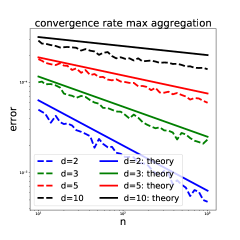
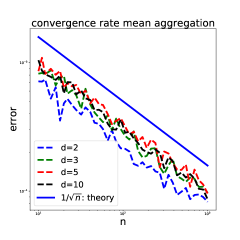
Figure 1. For both figures, the dashed lines represent the experimental error as the graph size increases, while the full lines represent the theoretical rates arising from Ths. 5.7 and 5.12. This experiment has been conducted for various values of the latent space dimension $d$. The theoretical rates are $1/\sqrt{n}$ for a mean aggregation and $1/\sqrt[d]{n}$ for a max aggregation. The plots are log scaled and the full lines have manually been translated to improve readability.

6Conclusion

In this work, we have defined continuous counterparts of MPGNNs with very generic aggregation functions on a probability space with respect to a transition kernel. We then have shown that under certain conditions, cMPGNNs are limits of discrete MPGNNs on random graphs sampled from the corresponding random graph model. Until now, similar result were known for SGNNs, which are more restricted architectures, or for MPGNNs with a degree normalized mean aggregation. Our main contribution is to extend this to abstract MPGNNs with generic aggregation functions. All along this paper, a focus is given on examples based on mean or weighted mean aggregation (Examples 1, 2 and 3) and max aggregation (Example 4), but our theorems are not limited to these examples and is in fact verified for mild assumptions on the underlying model.

Throughout this paper, we have emphasized the fact that mean and max aggregation behave differently. Albeit, a link between the two still exists. One could consider an aggregation function using a $L_{p}$-mean (a.k.a. generalized mean, or power mean, or also Hölder mean). In this setup, assuming positive values everywhere, the mean and max aggregation correspond to the cases $p=1$ and $p=\infty$, respectively. Nevertheless, a straightforward application of the McDiarmid inequality for a $L_{p}$-mean MPGNN would give a convergence rate that involves $O(1/\sqrt[p]{n})$, and this does not match with the case $p=\infty$, for which we obtained a rate in $O(1/\sqrt[d]{n})$ using a different concentration bound. Future work could try to come up with a proof on $L_{p}$, which could unify the two approaches described in this paper.

Appendices

7Proof of Theorem 5.7

7.1Equivariant case

We start with the equivariant case. We seek to bound:

$$\operatorname{MAE}_{X}\left(\Theta_{G_{n}}(S_{X}(f)),\Theta_{W,P}(f)\right) =\max_{1\leq i\leq n}\left\|(S_{X}f)^{(L)}_{i}-S_{X}(f^{(L)})_{i}\right\|$$

$$=\max_{1\leq i\leq n}\left\|(S_{X}f)^{(L)}_{i}-f^{(L)}(X_{i})\right\|.$$

We will prove the following sharper version of Theorem 5.7.

Theorem 7.1.

Under same assumptions that Theorem 5.7 Let $\rho>0$, then with probability at least $1-\rho$:

(7.1) $$\begin{split}&\max_{1\leq i\leq n}\left\|(S_{X}f)^{(L)}_{i}-f^{(L)}(X_{i})\right\|\\ &\leq\sum_{l=1}^{L}A_{n}^{(l,L)}\left[D_{n}^{(l)}\sqrt{\frac{1}{2}n\ln\left(\frac{2^{L+2-l}nd_{l}}{\rho}\right)}+a_{n-1}^{(l)}\right]\end{split}$$

Where $A_{n}^{(l,L)}=\prod_{k=l+1}^{L}(\mu_{F}^{(k)}+\lambda_{F,n-1}^{(k)})$ with the conventions $\prod_{k=a}^{b}(\dots)=1$ and $\sum_{k=a}^{b}(\dots)=0$ if $a>b$.

Then Theorem 5.7 in the main text is actually the following corollary.

Corollary 7.2 (Theorem 5.7 in the main text).

With probability at least $1-\rho$:

$$\max_{i}\left\|(S_{X}f)^{(L)}_{i}-f^{(L)}(X_{i})\right\|_{\infty}\lesssim LD_{n}\sqrt{n\ln\left(\frac{n2^{L}d_{max}}{\rho}\right)}+La_{n}.$$

Proof.

The $A_{n}^{(l,L)}=\prod_{k=l+1}^{L}(\mu_{F}^{(k)}+\lambda_{F,n-1}^{(k)})$ are bounded over $n$ by assumption. Thus, the corollary comes directly from Theorem 7.1. ∎

Proof of Theorem 7.1.

We prove the result by induction on $L$. Let $\rho>0$, until the end of this proof we denote by $H^{(L)}(\rho)$ the bound (7.1):

$$H^{(L)}(\rho)=\sum_{l=1}^{L}A_{n}^{(l,L)}\left[D_{n}^{(l)}\sqrt{\frac{1}{2}n\ln\left(\frac{2^{L+2-l}nd_{l}}{\rho}\right)}+a_{n-1}^{(l)}\right].$$

We recall those notations from Definition 5.2

$$F_{P,n}^{(l+1)}(f^{(l)},W)(x)$$

$$=\mathbb{E}_{X_{1},\dots,X_{n}}\left[F^{(l+1)}\left(f^{(l)}(x),\{\!\!\{\left(f^{(l)}(X_{k}),W(x,X_{k})\right)\}\!\!\}_{1\leq k\leq n}\right)\right],$$

and,

$$\mathcal{F}_{P}^{(l+1)}(f^{(l)},W)(x)=\mathcal{F}^{(l+1)}_{P}\left(f^{(l)}(x),\left(f^{(l)},W(x,\cdot)\right)\right)=f^{(l+1)}(x).$$

Suppose $L=1$, we shall find a quantity that bounds all the $\left\|(S_{X}f)^{(1)}_{i}-f^{(1)}(X_{i})\right\|$ for $i=1,\dots,n$ with probability at least $1-\rho/n$. Thereby, by a union bound, this quantity will bound their maximum with probability at least $1-\rho$.

Choose $i\in\{1,\dots,n\}$ and $x_{i}\in\mathcal{X}$, consider

$$\left\|F^{(1)}\left(f^{(0)}(x_{i}),\{\!\!\{\left(f^{(0)}(X_{k}),W(x_{i},X_{k})\right)\}\!\!\}_{k\neq i}\right)-f^{(1)}(x_{i})\right\|_{\infty}.$$

From a triangular inequality,

(7.2) $$\begin{split}&\left\|F^{(1)}\left(f^{0)}(x_{i}),\{\!\!\{\left(f^{(0)}(X_{k}),W(x_{i},X_{k})\right)\}\!\!\}_{k\neq i}\right)-f^{(1)}(x_{i})\right\|_{\infty}\\ &\leq\left\|F^{(1)}\left(f^{(0)}(x_{i}),\{\!\!\{\left(f^{(0)}(X_{k}),W(x_{i},X_{k})\right)\}\!\!\}_{k\neq i}\right)-F_{P,n-1}^{(1)}(f^{(0)},W)(x_{i})\right\|_{\infty}\\ &\qquad+\left\|F_{P,n-1}^{(1)}(f^{(0)},W)(x_{i})-f^{(1)}(x_{1})\right\|_{\infty}\\ &\leq\left\|F^{(1)}\left(f^{(0)}(x_{i}),\{\!\!\{\left(f^{(0)}(X_{k}),W(x_{i},X_{k})\right)\}\!\!\}_{k\neq i}\right)-F_{P,n-1}^{(1)}(f^{(0)},W)(x_{i})\right\|_{\infty}\\ &\qquad+a_{n-1}^{(1)}.\end{split}$$

by definition of $a_{n}$. Now we bound (7.2) with high probability using McDiarmid’s inequality 10.2 on

$$F^{(1)}\left(f^{(0)}(x_{i}),\{\!\!\{\left(f^{(0)}(x_{k}),W(x_{i},x_{k})\right)\}\!\!\}_{k\neq i}\right)$$

as a multivariate function of the $n-1$ variables $x_{2},\dots,x_{n}$.

We obtain that for any $x_{1}$, with probability at least $1-\rho/n$,

(7.3) $$\begin{split}&\left\|F^{(1)}\left(f^{(0)}(x_{i}),\{\!\!\{\left(f^{(0)}(X_{k}),W(x_{i},X_{k})\right)\}\!\!\}_{k\neq i}\right)-f^{(1)}(x_{1})\right\|_{\infty}\\ &\leq D_{n}^{(1)}\sqrt{\frac{1}{2}(n-1)\ln\left(\frac{2d_{1}n}{\rho}\right)}+a_{n-1}^{(1)}\\ &\leq D_{n}^{(1)}\sqrt{\frac{1}{2}n\ln\left(\frac{2d_{1}n}{\rho}\right)}+a_{n-1}^{(1)}.\end{split}$$

Hence, by conditioning over $X_{i}$ and applying the law of total probability, (7.3) yields with probability at least $1-\rho/n$:

(7.4) $$\left\|(S_{X}f)^{(1)}_{i}-f^{(1)}(X_{i})\right\|_{\infty}\leq D_{n}^{(1)}\sqrt{\frac{1}{2}n\ln\left(\frac{2d_{1}n}{\rho}\right)}+a_{n-1}^{(1)}.$$

And by a union bound, we can conclude that with probability at least $1-\rho$:

(7.5) $$\max_{i}\left\|(S_{X}f)^{(1)}_{i}-f^{(1)}(X_{i})\right\|_{\infty}\leq D_{n}^{(1)}\sqrt{\frac{1}{2}n\ln\left(\frac{2d_{1}n}{\rho}\right)}+a_{n-1}^{(1)}\leq H^{(1)}(\rho).$$

Now suppose the theorem true for $L\geq 1$. For any node $i$,

$$\left\|(S_{X}f)^{(L+1)}_{i}-f^{(L+1)}(X_{i})\right\|_{\infty}$$

$$\leq\left\|(S_{X}f)^{(L+1)}_{i}-F_{P,n-1}^{(L+1)}(f^{(L)},W)(X_{i})\right\|_{\infty}$$

$$\quad+\left\|F_{P,n-1}^{(L+1)}(f^{(L)},W)(X_{i})+f^{(L+1)}(X_{i})\right\|_{\infty}$$

$$\leq\left\|(S_{X}f)^{(L+1)}_{i}-F_{P,n-1}^{(L+1)}(f^{(L)},W)(X_{i})\right\|_{\infty}+a_{n-1}^{(L+1)}$$

$$\leq\left\|(S_{X}f)^{(L+1)}_{i}-F^{(L+1)}\left(f^{(L)}(X_{i}),\{\!\!\{\left(f^{(L)}(X_{k}),W(X_{i},X_{k})\right)\}\!\!\}_{k\neq i}\right)\right\|_{\infty}$$

$$\quad+\left\|F^{(L+1)}\left(f^{(L)}(X_{i}),\{\!\!\{\left(f^{(L)}(X_{k}),W(X_{i},X_{k})\right)\}\!\!\}_{k\neq i}\right)-F_{P,n-1}^{(L+1)}(f^{(L)},W)(X_{i})\right\|_{\infty}$$

$$\quad+a_{n-1}^{(L+1)}$$

$$\leq\mu_{F}^{(L+1)}\left\|(S_{X}f)^{(L)}_{i}-f^{(L)}(X_{i})\right\|_{\infty}+\lambda_{F,n-1}^{(L+1)}\max_{j\neq i}\left\|(S_{X}f)^{(L)}_{j}-f^{(L)}(X_{j})\right\|_{\infty}$$

$$\quad+\left\|F^{(L+1)}\left(f^{(L)}(X_{i}),\{\!\!\{\left(f^{(L)}(X_{k}),W(X_{i},X_{k})\right)\}\!\!\}_{k\neq i}\right)-F_{P,n-1}^{(L+1)}(f^{(L)},W)(X_{i})\right\|_{\infty}$$

(7.6) $$\quad+a_{n-1}^{(L+i)}.$$

Where the last inequality comes from the Lipschitz-like regularity Assumption 5.6 (iv) on $F^{(L+1)}$. Now taking the maximum over the vertices:

$$\max_{i}\left\|(S_{X}f)^{(L+1)}_{i}-f^{(L+1)}(X_{i})\right\|_{\infty}$$

$$\leq\mu_{F}^{(L+1)}\max_{i}\left\|(S_{X}f)^{(L)}_{i}-f^{(L)}(X_{i})\right\|$$

$$\quad+\lambda_{F,n-1}^{(L+1)}\max_{i}\max_{j\neq i}\left\|{}_{\infty}(S_{X}f)^{(L)}_{j}-f^{(L)}(X_{j})\right\|_{\infty}$$

$$\quad+\max_{i}\left\|F^{(L+1)}\left(f(X_{i}),\{\!\!\{\left(f(X_{k}),W(X_{i},X_{k})\right)\}\!\!\}_{k\neq i}\right)-F_{P,n-1}^{(L+1)}(f^{(L)},W)(X_{i})\right\|_{\infty}$$

$$\quad+a_{n-1}^{(L+1)}$$

$$\leq(\mu_{F}^{(L+1)}+\lambda_{F,n-1}^{(L+1)})\max_{i}\left\|(S_{X}f)^{(L)}_{i}-f^{(L)}(X_{i})\right\|_{\infty}$$

$$\quad+\max_{i}\left\|F^{(L+1)}\left(f(X_{i}),\{\!\!\{\left(f(X_{k}),W(X_{i},X_{k})\right)\}\!\!\}_{k\neq i}\right)-F_{P,n-1}^{(L+1)}(f^{(L)},W)(X_{i})\right\|_{\infty}$$

(7.7) $$\quad+a_{n-1}^{(L+1)}$$

because $\max_{i}\max_{j\neq i}a_{i}=\max_{i}a_{i}$.

Finally, we bound (7.7) with high probability. The first term is handled by the induction hypothesis. For the second term, by conditioning over $X_{i}$, using McDiarmid and a union bound, the same way we did in the case $L=1$, we obtain with probability at least $1-\rho$:

$$\max_{i}\left\|(S_{X}f)^{(L+1)}_{i}-f^{(L+1)}(X_{i})\right\|_{\infty}$$

$$\leq(\mu_{F}^{(L+1)}+\lambda_{F,n-1}^{(L+1)})H^{(L)}(\rho/2)+D_{n}^{(L+1)}\sqrt{\frac{1}{2}n\ln\left(\frac{4d_{L+1}n}{\rho}\right)}+a_{n-1}^{(L+1)}$$

$$=\sum_{l=2}^{L}(\mu_{F}^{(L+1)}+\lambda_{F,n-1}^{(L+1)})A_{n}^{(l,L)}D_{n}^{(l)}\sqrt{\frac{1}{2}n\ln\left(\frac{2^{L+1+2-l}nd_{l}}{\rho}\right)}$$

$$\quad+(\mu_{F}^{(L+1)}+\lambda_{F,n-1}^{(L+1)})A_{n}^{(1,L)}D_{n}^{(1)}\sqrt{\frac{1}{2}n\ln\left(\frac{2^{L+1}nd_{1}}{\rho}\right)}$$

$$\quad+(\mu_{F}^{(L+1)}+\lambda_{F,n-1}^{(L+1)})\sum_{l=1}^{L}A_{n}^{(l,L)}a_{n-1}^{(l)}+D_{n}^{(L+1)}\sqrt{\frac{1}{2}n\ln\left(\frac{4d_{L+1}n}{\rho}\right)}+a_{n-1}^{(L+1)}$$

$$=\sum_{l=2}^{L}A_{n}^{(l,L+1)}D_{n}^{(l)}\sqrt{\frac{1}{2}n\ln\left(\frac{2^{L+1+2-l}nd_{l}}{\rho}\right)}$$

$$\quad+A_{n}^{(1,L+1)}D_{n}^{(1)}\sqrt{\frac{1}{2}n\ln\left(\frac{2^{L+1}nd_{1}}{\rho}\right)}$$

$$\quad+\sum_{l=1}^{L}A_{n}^{(l,L+1)}a_{n-1}^{(l)}+D_{n}^{(L+1)}\sqrt{\frac{1}{2}n\ln\left(\frac{4d_{L+1}n}{\rho}\right)}+a_{n-1}^{(L+1)}$$

$$=\sum_{l=2}^{L+1}A_{n}^{(l,L+1)}D_{n}^{(l)}\sqrt{\frac{1}{2}n\ln\left(\frac{2^{L+1+2-l}nd_{l}}{\rho}\right)}$$

$$\quad+A_{n}^{(1,L+1)}D_{n}^{(1)}\sqrt{\frac{1}{2}n\ln\left(\frac{2^{L+1}nd_{1}}{\rho}\right)}+\sum_{l=1}^{L+1}A_{n}^{(l,L+1)}a_{n-1}^{(l)}$$

$$\leq\sum_{l=1}^{L+1}A_{n}^{(l,L+1)}\left[D_{n}^{(l)}\sqrt{\frac{1}{2}n\ln\left(\frac{2^{L+1+2-l}nd_{l}}{\rho}\right)}+a_{n-1}^{(l)}\right]$$

$$=H^{(L+1)}(\rho).$$

∎

7.2Invariant case

For the invariant case, we use the bound of the equivariant case previously obtained, and we make an additional use of McDiarmid’s concentration bound.

Proof.

(7.8) $$\begin{split}&\left\|\bar{\Theta}_{G_{n}}(S_{X}(f))-\bar{\Theta}_{W,P}(f)\right\|_{\infty}\\ &\leq\left\|R\left(\{\!\!\{(S_{X}f)^{(L)}_{1},\dots,(S_{X}f)_{n}^{(L)}\}\!\!\}\right)-R\left(\{\!\!\{f^{(L)}(X_{1}),\dots,f^{(L)}(X_{n})\}\!\!\}\right)\right\|_{\infty}\\ &\quad+\left\|R\left(\{\!\!\{f^{(L)}(X_{1}),\dots,f^{(L)}(X_{n})\}\!\!\}\right)-R_{P,n}(f^{(L)})\right\|_{\infty}\\ &\quad+\left\|R_{P,n}(f^{(L)})-\mathcal{R}_{P}(f^{(L)})\right\|_{\infty}\\ &\leq\lambda_{R,n}\max_{i}\left\|(S_{X}f)^{(L)}_{i}-f^{(L)}(X_{i})\right\|_{\infty}\\ &\quad+\left\|R\left(\{\!\!\{f^{(L)}(X_{1}),\dots,f^{(L)}(X_{n})\}\!\!\}\right)-R_{P,n}(f^{(L)})\right\|_{\infty}+b_{n}\end{split}$$

Using the bound of the equivariant case, McDiarmid’s inequality and the fact that $(\lambda_{R,n})$ is bounded, we get that, with probability at least $1-\rho$:

$$\begin{split}\left\|\bar{\Theta}_{G_{n}}(S_{X}(f))-\bar{\Theta}_{W,P}(f)\right\|_{\infty}&\lesssim LD_{n}\sqrt{n\ln\left(\frac{n2^{L+1}d_{max}}{\rho}\right)}+C_{n}\sqrt{n\ln\left(\frac{4d_{L}}{\rho}\right)}\\ &\quad+La_{n-1}+b_{n}\end{split}$$

∎

8Proof of Theorem 5.12

We will need the following property.

Proposition 8.1.

Under the hypothesis of Theorem 5.12, The functions $f^{(0)},\dots,f^{(L)}$ are Lipschitz continuous. We denote by $\lambda_{f}=\lambda_{f^{(0)}},\dots,\lambda_{f^{(L)}}$ their Lipschitz constants.

Proof.

It is already assumed for $l=0$. Suppose it is true for $l\geq 1$, $f^{(l+1)}(x)=\sup_{y}W(x,y)\psi^{(l+1)}(f^{(l)}(y))=\sup_{y}g(x,y)$ where $g$ is $\lambda_{W}\|\psi^{(l+1)}\circ f^{(l)}\|_{\infty}+\lambda_{\psi^{(l)}}\lambda_{f^{(l)}}$ Lipschitz. Then from Lemma 10.5 $f^{(l+1)}$ is also Lipschitz. ∎

8.1Equivariant case

We will prove the following sharper version of Theorem 5.12

Theorem 8.2.

Suppose, $(\mathcal{X},P)$ has the $(r_{0},\kappa)$-volume retaining property and that $f,W$ and the $\psi^{(l)}$ are Lipschitz continuousLet $\rho\geq 2^{L-1}ne^{-n\kappa r_{0}^{d}2^{d}}$ and $n$ large enough for $0<\rho<1$ to hold. Then with probability at least $1-\rho$:

(8.1) $$\begin{split}&\max_{1\leq i\leq n}\left\|(S_{X}f)^{(L)}_{i}-f^{(L)}(X_{i})\right\|_{\infty}\\ &\leq\sum_{l=1}^{L}B^{(l,L)}\frac{\lambda_{f^{(l)}}}{2}\left(\frac{1}{n\kappa}\ln\left(\frac{2^{L+1-l}nd_{l}}{\rho}\right)\right)^{1/d}\end{split}$$

Where $B^{(l,L)}=\prod_{k=l+1}^{L}\lambda_{\psi^{(k)}}$ with the conventions $\prod_{k=a}^{b}=1$ and $\sum_{k=a}^{b}=0$ if $a>b$.

Corollary 8.3 (Theorem 5.12 in the main text).

Suppose, $(\mathcal{X},P)$ has the $(r_{0},\kappa)$-volume retaining property and that $f,W$ and the $\psi^{(l)}$ are Lipschitz continuous. Let $\rho\geq 2^{L-1}ne^{-n\kappa r_{0}^{d}2^{d}}$ and $n$ large enough for $0<\rho<1$ to hold. Then with probability at least $1-\rho$:

$$\max_{1\leq i\leq n}\left\|(S_{X}f)^{(L)}_{i}-f^{(L)}(X_{i})\right\|_{\infty}\lesssim L\left(\frac{1}{n}\ln\left(\frac{2^{L-1}nd_{\max}}{\rho}\right)\right)^{1/d}$$

Proof of theorem 8.2.

Let $\rho>0$. We will prove the theorem by induction on $L$. Until the end of the proof, we denote by $H^{(L)}(\rho)$ the bound (8.1):

$$H^{(L)}(\rho)=\sum_{l=1}^{L}B^{(l,L)}\frac{\lambda_{f^{(l)}}}{2}\left(\frac{1}{n\kappa}\ln\left(\frac{2^{L+1-l}nd_{l}}{\rho}\right)\right)^{1/d}.$$

For $L=1$, let us note $g(x,y)=W(x,y)\psi^{(1)}(f^{(0)}(y))$. The map $g$ is $\lambda_{f^{(1)}}=\lambda_{\psi^{(1)}}\lambda_{f^{(0)}}+\|\psi^{(1)}\circ f^{(0)}\|_{\infty}\lambda_{W}$ Lipschitz continuous from Property 8.1. Fix $i\in\{1,\dots,n\}$ and $x_{i}\in\mathcal{X}$, by lemma 5.11, for $\rho\geq ne^{-n\kappa r_{0}^{d}2^{d}}$, with probability at least $1-\rho/n$, we have

$$\left\|\max_{j\neq i}g(x,X_{j})-\sup_{y\in\mathcal{X}}g(x,y)\right\|_{\infty}\leq\frac{\lambda_{f^{(1)}}}{2}\left(\frac{1}{(n-1)\kappa}\ln\left(\frac{nd_{0}}{\rho}\right)\right)^{1/d}\qquad\forall x\in\mathcal{X}.$$

Thus, by the law of total probability, with probability at least $1-\rho/n$,

$$\left\|\max_{j\neq i}g(X_{i},X_{j})-\sup_{y\in\mathcal{X}}g(X_{i},y)\right\|_{\infty}\leq\frac{\lambda_{f^{(1)}}}{2}\left(\frac{1}{(n-1)\kappa}\ln\left(\frac{nd_{0}}{\rho}\right)\right)^{1/d}.$$

And by maximizing over $i$ and doing a union bound, for $\rho\geq ne^{-n\kappa r_{0}^{d}2^{d}}$, with probability at least $1-\rho$:

$$\max_{i}\left\|(S_{X}f)^{(1)}_{i}-f^{(1)}(X_{i})\right\|_{\infty}\leq\frac{\lambda_{f^{(1)}}}{2}\left(\frac{1}{(n-1)\kappa}\ln\left(\frac{nd_{0}}{\rho}\right)\right)^{1/d}\leq H^{(1)}(\rho).$$

That concludes the case $L=1$. Now let $L\geq 1$, fix $i\in\{1,\dots,n\}$:

(8.2) $$\begin{split}&\left\|(S_{X}f)^{(L+1)}_{i}-f^{(L+1)}(X_{i})\right\|_{\infty}\\ &=\left\|\max_{j\neq i}W(X_{i},X_{j})\psi^{(L+1)}((S_{X}f)^{(L)}_{j})-f^{(L+1)}(X_{j})\right\|_{\infty}\\ &\leq\left\|\max_{j\neq i}W(X_{i},X_{j})\psi^{(L+1)}((S_{X}f)^{(L)}_{j})-\max_{j\neq i}W(X_{i},X_{j})\psi^{(L+1)}(f^{(L)}(X_{j}))\right\|_{\infty}\\ &\quad+\left\|\max_{j\neq i}W(X_{i},X_{j})\psi^{(L+1)}(f^{(L)}(X_{j}))-\sup_{y\in\mathcal{X}}W(X_{i},y)\psi^{(L+1)}(f^{(L)}(y))\right\|_{\infty}\\ &\leq\lambda_{\psi^{(L+1)}}\max_{j\neq i}\left\|(S_{X}f)^{(L)}_{j}-f^{(L)}(X_{j})\right\|_{\infty}\\ &\quad+\left\|\max_{j\neq i}W(X_{i},X_{j})\psi^{(L+1)}(f^{(L)}(X_{j}))-\sup_{y\in\mathcal{X}}W(X_{i},y)\psi^{(L+1)}(f^{(L)}(y))\right\|_{\infty}\\ \end{split}$$

Where the last inequality uses Lemma 10.4, $|W|\leq 1$, and Lipschitz continuity of $\psi^{(L+1)}$. Thus taking the maximum over $i$:

(8.3) $$\begin{split}&\max_{i}\left\|(S_{X}f)^{(L+1)}_{i}-f^{(L+1)}(X_{i})\right\|_{\infty}\\ &\leq\lambda_{\psi^{(L+1)}}\max_{i}\left\|(S_{X}f)^{(L)}_{j}-f^{(L)}(X_{j})\right\|_{\infty}\\ &\quad+\max_{i}\left\|\max_{j\neq i}W(X_{i},X_{j})\psi^{(L+1)}(f^{(L)}(X_{j}))-\sup_{y\in\mathcal{X}}W(X_{i},y)\psi^{(L+1)}(f^{(L)}(y))\right\|_{\infty}\\ \end{split}$$

Now we bound (8.3) with high probability. We use the induction hypothesis for the first term. For the second term, we set $g(x,y)=W(x,y)\psi^{(L+1)}(f^{(L)}(y))$ and use lemma 5.11 on $g$ which is $\lambda_{f^{(L+1)}}=\lambda_{\psi^{(L+1)}}\lambda_{f^{(L)}}+\|\psi^{(L+1)}\circ f^{(L)}\|_{\infty}\lambda_{W}$ Lipschitz. The method is the same as in the case $L=1$ and by conditioning over $X_{i}$ followed by a union bound. We obtain that for $\rho\geq 2^{L}ne^{-n\kappa r_{0}^{d}2^{d}}$, with probability at least $1-\rho$:

$$\max_{i}\left\|(S_{X}f)^{(L+1)}_{i}-f^{(L+1)}(X_{i})\right\|_{\infty}$$

$$\leq\lambda_{\psi^{(L+1)}}H^{(L)}(\rho/2)+\frac{\lambda_{f^{(L+1)}}}{2}\left(\frac{1}{(n-1)\kappa}\ln\left(\frac{2nd_{L}}{\rho}\right)\right)^{1/d}$$

$$=\sum_{l=2}^{L}\lambda_{\psi^{(L+1)}}B^{(l,L)}\frac{\lambda_{f^{(l)}}}{2}\left(\frac{1}{(n-1)\kappa}\ln\left(\frac{2^{L+2-l}nd_{l}}{\rho}\right)\right)^{1/d}$$

$$\quad+\lambda_{\psi^{(L+1)}}B^{(1,L)}\frac{\lambda_{f^{(1)}}}{2}\left(\frac{1}{(n-1)\kappa}\ln\left(\frac{2^{L}nd_{0}}{\rho}\right)\right)^{1/d}$$

$$\quad+\frac{\lambda_{f^{(L+1)}}}{2}\left(\frac{1}{(n-1)\kappa}\ln\left(\frac{2nd_{L}}{\rho}\right)\right)^{1/d}$$

$$=\sum_{l=2}^{L}B^{(l,L+1)}\frac{\lambda_{f^{(l)}}}{2}\left(\frac{1}{(n-1)\kappa}\ln\left(\frac{2^{L+2-l}nd_{l}}{\rho}\right)\right)^{1/d}$$

$$\quad+B^{(1,L+1)}\frac{\lambda_{f^{(1)}}}{2}\left(\frac{1}{(n-1)\kappa}\ln\left(\frac{2^{L}nd_{0}}{\rho}\right)\right)^{1/d}$$

$$\quad+\frac{\lambda_{f^{(L+1)}}}{2}\left(\frac{1}{(n-1)\kappa}\ln\left(\frac{2nd_{L}}{\rho}\right)\right)^{1/d}$$

$$=\sum_{l=2}^{L+1}B^{(l,L+1)}\frac{\lambda_{f^{(l)}}}{2}\left(\frac{1}{(n-1)\kappa}\ln\left(\frac{2^{L+2-l}nd_{l}}{\rho}\right)\right)^{1/d}$$

$$\quad+B^{(1,L+1)}\frac{\lambda_{f^{(1)}}}{2}\left(\frac{1}{(n-1)\kappa}\ln\left(\frac{2^{L}nd_{0}}{\rho}\right)\right)^{1/d}$$

$$\leq H^{(L+1)}(\rho).$$

∎

8.2Invariant case

Theorem 8.4.

Suppose, $(\mathcal{X},P)$ has the $(r_{0},\kappa)$-volume retaining property and that $f,W$ and the $\psi^{(l)}$ are Lipschitz continuous. Let $\rho\geq 2^{L-1}ne^{-n\kappa r_{0}^{d}2^{d}}$ and $n$ large enough for $0<\rho<1$ to hold. Then with probability at least $1-\rho$:

$$\left\|\bar{\Theta}_{G_{n}}(S_{X}(f))-\bar{\Theta}_{W,P}(f)\right\|_{\infty}\lesssim L\left(\frac{1}{n-1}\ln\left(\frac{2^{L}nd_{\max}}{\rho}\right)\right)^{1/d}+\left(\frac{1}{n}\ln\left(\frac{2d_{L}}{\rho}\right)\right)^{1/d}.$$

Proof.

$$\begin{split}&\left\|\bar{\Theta}_{G_{n}}(S_{X}(f))-\bar{\Theta}_{W,P}(f)\right\|_{\infty}=\left\|\max_{i}(S_{X}f)_{i}^{(L)}-\sup f^{(L)}\right\|_{\infty}\\ &\leq\left\|\max_{i}(S_{X}f)_{i}^{(L)}-\max_{i}f^{(L)}(X_{i})\right\|_{\infty}+\left\|\max_{i}f^{(L)}(X_{i})-\sup f^{(L)}\right\|_{\infty}\\ &\leq\max_{i}\left\|(S_{X}f)^{(L)}_{i}-f^{(L)}(X_{i})\right\|_{\infty}+\left\|\max_{i}f^{(L)}(X_{i})-\sup f^{(L)}\right\|_{\infty}.\end{split}$$

Using the bound for the equivariant case and Lemma 5.11 on $f^{(L)}$, we obtain the result. ∎

9Examples

For notational convenience, we drop any subscript or superscript referring to layers. Recall that $\psi$ is supposed Lipschitz and bounded, we denote $\lambda_{\psi}$ its Lipschitz constant and $\|\psi\|_{\infty}=\sup_{x}\|\psi(x)\|_{\infty}$. For Examples 1, 2 and 3,

• We check Assumptions 5.6.

• We compute the $a_{n}$ from (5.17).

• We compute the bounded differences

For Example 4, we show that the bounded differences are not sharp enough.

9.1Examples 1 and a: Convolutional message passing with mean aggregation

Check of Assumptions 5.6.

Let $x,x^{\prime}\in\mathbb{R}^{d_{l-1}}$ and $m=\{\!\!\{(y_{i},t_{i}),\}\!\!\}_{1\leq i\leq n},m^{\prime}=\{\!\!\{(y_{i}^{\prime},t_{i}^{\prime})\}\!\!\}_{1\leq i\leq n}\subset\mathbb{R}^{d_{l-1}}\times[0,1]$.

$$\begin{split}&\left\|F(x,m)-F(x^{\prime},m^{\prime})\right\|_{\infty}\leq\frac{1}{n}\sum_{1\leq i\leq n}\left\|t_{i}\psi(y_{i})-t_{i}^{\prime}\psi(y_{i}^{\prime})\right\|_{\infty}\\ &\leq\frac{1}{n}\sum_{1\leq i\leq n}\left\|t_{i}\psi(y_{i})-t_{i}\psi(y_{i}^{\prime})\right\|_{\infty}+\left\|t_{i}\psi(y_{i}^{\prime})-t_{i}^{\prime}\psi(y_{i}^{\prime})\right\|_{\infty}\\ &\leq\frac{1}{n}\sum_{1\leq i\leq n}\lambda_{\psi}\left\|y_{i}-y_{i}^{\prime}\right\|+\|\psi\|_{\infty}\left|t_{i}-t_{i}^{\prime}\right|\\ &\leq\max\left(\lambda_{\psi},\|\psi\|_{\infty}\right)\max_{1\leq i\leq n}\|y_{i}-y_{i}^{\prime}\|_{\infty}+|t_{i}-t_{i}^{\prime}|.\end{split}$$

This inequality does not depend on any ordering of the $(y_{i}^{\prime},t_{i}^{\prime})$ so that

$$\left\|F(x,m)-F(x^{\prime},m^{\prime})\right\|_{\infty}\leq\max\left(\lambda_{\psi},\|\psi\|_{\infty}\right)\max_{1\leq i\leq n}\|y_{i}-y_{\sigma(i)}^{\prime}\|_{\infty}+|t_{i}-t_{\sigma(i)}^{\prime}|$$

for any permutation $\sigma$. Taking the minimum over $S_{n}$ we get the Assumption with $\mu_{F}=0$ and $\lambda_{F,n}=\max\left(\lambda_{\psi},\|\psi\|_{\infty}\right)$ which is bounded over $n$.

Calculation of $a_{n}$

By linearity of the expected value, it is clear that for any $X_{1},\dots,X_{n}\overset{iid}{\sim}P$ and any $f$,

$$\mathbb{E}\left[\frac{1}{n}\sum_{i}W(x,X_{i})\psi(X_{i})\right]=\mathbb{E}\left[W(x,X_{1})\psi(X_{1})\right]=\int_{\mathcal{X}}W(x,y)\psi(y)dP(y)\quad\forall x$$

So $a_{n}=0$.

Calculation of bounded differences $\mathbf{D_{n}}$.

Let $x_{1},x_{n}$ and $x_{2}^{\prime},\dots,x_{n}^{\prime}$ be such that $x_{i}=x_{i}^{\prime}$ except at $i=2$

$$\begin{split}&\left\|F\left(f(x_{1}),\{\!\!\{\left(f(x_{k}),W(x_{1},x_{k})\right)\}\!\!\}_{2\leq k\leq n}\right)-F\left(f(x_{1}),\{\!\!\{\left(f(x_{k}^{\prime}),W(x_{1},x_{k}^{\prime})\right)\}\!\!\}_{2\leq k\leq n}\right)\right\|_{\infty}\\ &=\frac{1}{n-1}\left\|W(x_{1},x_{2})\psi(f(x_{2}))-W(x_{1},x_{2}^{\prime})\psi^{(l)}(f(x_{2}^{\prime}))\right\|\\ &=O(1/n).\end{split}$$

Since $\psi\circ f$ is bounded.

9.2Example 2 and b: Degree normalized convolutional message passing with sum aggregation

We make the additional assumption that there exists $\alpha>0$ such that $W(x,y)>\alpha,\ \forall x,y$.

Check of Assumption 5.6.

Let $x,x^{\prime}\in\mathbb{R}^{d}$ and $m=\{\!\!\{(y_{i},t_{i}),\}\!\!\}_{1\leq i\leq n},m^{\prime}=\{\!\!\{(y_{i}^{\prime},t_{i}^{\prime})\}\!\!\}_{1\leq i\leq n}\subset\mathbb{R}^{d_{l-1}}\times[\alpha,1]$.

$$\left\|F(x,m)-F(x^{\prime},m^{\prime})\right\|_{\infty}\leq\sum_{1\leq i\leq n}\left\|\frac{t_{i}\psi(y_{i})}{\sum_{k}t_{k}}-\frac{t_{i}^{\prime}\psi(y_{i})}{\sum_{k}t_{k}^{\prime}}\right\|_{\infty}$$

$$=\sum_{1\leq i\leq n}\left\|\frac{\sum_{k}t_{k}^{\prime}t_{i}\psi(y_{i})-\sum_{k}t_{k}t_{i}^{\prime}\psi(y_{i}^{\prime})}{\sum_{k}t_{k}\sum_{k}t_{k}^{\prime}}\right\|_{\infty}$$

$$\leq\frac{1}{n^{2}\alpha^{2}}\sum_{1\leq i,k\leq n}\|t_{k}^{\prime}t_{i}\psi(y_{i})-t_{k}t_{i}^{\prime}\psi(y_{i}^{\prime})\|_{\infty}$$

$$\leq\frac{1}{n^{2}\alpha^{2}}\sum_{1\leq i,k\leq n}\left\|t_{k}^{\prime}t_{i}\psi(y_{i})-t_{k}^{\prime}t_{i}^{\prime}\psi(y_{i}^{\prime})\right\|_{\infty}+\left\|t_{k}^{\prime}t_{i}^{\prime}\psi(y_{i}^{\prime})-t_{k}t_{i}^{\prime}\psi(y_{i}^{\prime})\right\|_{\infty}$$

$$\leq\frac{1}{n^{2}\alpha^{2}}\sum_{1\leq i,k\leq n}\left\|t_{i}\psi(y_{i})-t_{i}^{\prime}\psi(y_{i}^{\prime})\right\|_{\infty}+\left\|t_{k}^{\prime}\psi(y_{i}^{\prime})-t_{k}\psi(y_{i}^{\prime})\right\|_{\infty}$$

$$\leq\frac{1}{n^{2}\alpha^{2}}\sum_{1\leq i,k\leq n}\left\|t_{i}\psi(y_{i})-t_{i}\psi(y_{i}^{\prime})\right\|_{\infty}+\left\|t_{i}\psi(y_{i}^{\prime})-t_{i}^{\prime}\psi(y_{i}^{\prime})\right\|_{\infty}+\|\psi\|_{\infty}|t_{k}-t_{k}^{\prime}|$$

$$\leq\frac{1}{n^{2}\alpha^{2}}\sum_{1\leq i,k\leq n}\lambda_{\psi}\left\|y_{i}-y_{i}^{\prime}\right\|_{\infty}+\|\psi\|_{\infty}|t_{i}-t_{i}^{\prime}|+\|\psi\|_{\infty}|t_{k}-t_{k}^{\prime}|$$

$$\leq\frac{1}{\alpha^{2}}\left(\lambda_{\psi}\max_{i}\left\|y_{i}-y_{i}^{\prime}\right\|_{\infty}+2\|\psi\|_{\infty}\max_{i}|t_{i}-t_{i}^{\prime}|\right)$$

$$=\frac{\max\left(\lambda_{\psi},2\|\psi\|_{\infty}\right)}{\alpha^{2}}\max_{1\leq i\leq n}\|y_{i}-y_{i}^{\prime}\|_{\infty}+|t_{i}-t_{i}^{\prime}|.$$

This inequality does not depend on any ordering of the $(y_{i}^{\prime},t_{i}^{\prime})$ so that

$$\left\|F(x,m)-F(x^{\prime},m^{\prime})\right\|_{\infty}\leq\frac{\max\left(\lambda_{\psi},2\|\psi\|_{\infty}\right)}{\alpha^{2}}\max_{1\leq i\leq n}\|y_{i}-y_{\sigma(i)}^{\prime}\|_{\infty}+|t_{i}-t_{\sigma(i)}^{\prime}|$$

for any permutation $\sigma$. Taking the minimum over $S_{n}$ we get the Assumption with $\mu_{F}=0$ and $\lambda_{F,n}=\frac{\max\left(\lambda_{\psi},2\|\psi\|_{\infty}\right)}{\alpha^{2}}$ which is bounded over $n$.

Calculation of $a_{n}$

This calculation has already been done in Example 2-b. We obtain $a_{n}=O(1/\sqrt{n})$.

Calculation of bounded differences $\mathbf{D_{n}}$.

Let $x_{1},\dots,x_{n}$ and $x_{2}^{\prime},\dots,x_{n}^{\prime}$ be such that $x_{i}=x_{i}^{\prime}$ except at $i=2$. This is the same calculation as the previous paragraph where $x=x^{\prime}=f(x_{1})$, $y_{i}=f(x_{i})$, $y_{i}^{\prime}=f(x_{i}^{\prime})$, $t_{i}=W(x_{1},x_{i})$ and $t_{i}^{\prime}=W(x_{1},x_{i}^{\prime})$ for $i\geq 2$. We get

$$\left\|F\left(f(x_{1}),\{\!\!\{\left(f(x_{k}),W(x_{1},x_{k})\right)\}\!\!\}_{2\leq k\leq n}\right)-F\left(f(x_{1}),\{\!\!\{\left(f(x_{k}^{\prime}),W(x_{1},x_{k}^{\prime})\right)\}\!\!\}_{2\leq k\leq n}\right)\right\|_{\infty}$$

$$\leq\frac{1}{(n-1)^{2}\alpha^{2}}\sum_{1\leq i,k\leq n-1}\lambda_{\psi}\left\|f(x_{i})-f(x_{i}^{\prime})\right\|_{\infty}+\|\psi\|_{\infty}|W(x_{1},x_{i})-W(x_{1},x_{i}^{\prime})|$$

$$\qquad+\|\psi\|_{\infty}|W(x_{1},x_{k})-W(x_{1},x_{k}^{\prime})|$$

$$=\frac{1}{(n-1)^{2}\alpha^{2}}((n-1)\lambda_{\psi}\left\|f(x_{2})-f(x_{2}^{\prime})\right\|_{\infty}+(n-1)\|\psi\|_{\infty}|W(x_{1},x_{2})-W(x_{1},x_{2}^{\prime})|$$

$$\qquad+(n-1)\|\psi\|_{\infty}|W(x_{1},x_{2})-W(x_{1},x_{2}^{\prime})|)$$

$$\leq\frac{2\lambda_{\psi}\|f\|_{\infty}+4\|\psi\|_{\infty}}{(n-1)\alpha^{2}}$$

$$=O(1/n)$$

$$=D_{n}.$$

So $D_{n}=O(1/n)$.

9.3Example 3 and c: Attentional message passing with sum aggregation

We make the additional assumption that there exists $\alpha,\beta>0$ and $\lambda_{c}>0$ such that $\alpha<c(x,y,t)<\beta$ and $|c(x,y,t)-c(x^{\prime},y^{\prime},t^{\prime})|\leq\lambda_{c}(\|x-x^{\prime}\|_{\infty}+\|y-y^{\prime}\|_{\infty}+|t-t^{\prime}|)$, $\forall x,x^{\prime},y,y^{\prime},t,t^{\prime}$. As a consequence, $c$ is bounded on any compact set.

Check of Assumption 5.6.

Let $x,x^{\prime}\in\mathbb{R}^{d}$ and $m=\{\!\!\{(y_{i},t_{i}),\}\!\!\}_{1\leq i\leq n},m^{\prime}=\{\!\!\{(y_{i}^{\prime},t_{i}^{\prime})\}\!\!\}_{1\leq i\leq n}\subset\mathbb{R}^{d_{l-1}}\times[0,1]$. Let us shorten $c(x,y_{i},t_{i})$ and $c(x,y_{i}^{\prime},t_{i}^{\prime})$ as $c_{i}$ and $c_{i}^{\prime}$.

$$\left\|F(x,m)-F(x^{\prime},m^{\prime})\right\|_{\infty}\leq\sum_{1\leq i\leq n}\left\|\frac{c_{i}\psi(y_{i})}{\sum_{k}c_{k}}-\frac{c_{i}^{\prime}\psi(y_{i})}{\sum_{k}c_{k}^{\prime}}\right\|_{\infty}$$

$$=\sum_{1\leq i\leq n}\left\|\frac{\sum_{k}c_{k}^{\prime}t_{i}\psi(y_{i})-\sum_{k}c_{k}c_{i}^{\prime}\psi(y_{i}^{\prime})}{\sum_{k}c_{k}\sum_{k}c_{k}^{\prime}}\right\|_{\infty}$$

$$\leq\frac{1}{n^{2}\alpha^{2}}\sum_{1\leq i,k\leq n}\|c_{k}^{\prime}c_{i}\psi(y_{i})-c_{k}c_{i}^{\prime}\psi(y_{i}^{\prime})\|_{\infty}$$

$$\leq\frac{1}{n^{2}\alpha^{2}}\sum_{1\leq i,k\leq n}\left\|c_{k}^{\prime}c_{i}\psi(y_{i})-c_{k}^{\prime}c_{i}^{\prime}\psi(y_{i}^{\prime})\right\|_{\infty}+\left\|c_{k}^{\prime}c_{i}^{\prime}\psi(y_{i}^{\prime})-c_{k}c_{i}^{\prime}\psi(y_{i}^{\prime})\right\|_{\infty}$$

$$\leq\frac{\beta}{n^{2}\alpha^{2}}\sum_{1\leq i,k\leq n}\left\|c_{i}\psi(y_{i})-c_{i}^{\prime}\psi(y_{i}^{\prime})\right\|_{\infty}+\left\|c_{k}^{\prime}\psi(y_{i}^{\prime})-c_{k}\psi(y_{i}^{\prime})\right\|_{\infty}$$

$$\leq\frac{\beta}{n^{2}\alpha^{2}}\sum_{1\leq i,k\leq n}\left\|c_{i}\psi(y_{i})-c_{i}\psi(y_{i}^{\prime})\right\|_{\infty}+\left\|c_{i}\psi(y_{i}^{\prime})-c_{i}^{\prime}\psi(y_{i}^{\prime})\right\|_{\infty}+\|\psi\|_{\infty}|c_{k}-c_{k}^{\prime}|$$

$$\leq\frac{\beta}{n^{2}\alpha^{2}}\sum_{1\leq i,k\leq n}\lambda_{\psi}\beta\left\|y_{i}-y_{i}^{\prime}\right\|_{\infty}+\|\psi\|_{\infty}|c_{i}-c_{i}^{\prime}|+\|\psi\|_{\infty}|c_{k}-c_{k}^{\prime}|$$

$$\leq\frac{\beta}{n^{2}\alpha^{2}}\sum_{1\leq i,k\leq n}\lambda_{\psi}\beta\left\|y_{i}-y_{i}^{\prime}\right\|_{\infty}+\|\psi\|_{\infty}\lambda_{c}(\|x-x^{\prime}\|_{\infty}+\|y_{i}-y_{i}^{\prime}\|_{\infty}+|t_{i}-t_{i}^{\prime}|)$$

$$\qquad\qquad\qquad\qquad+\|\psi\|_{\infty}\lambda_{c}(\|x-x^{\prime}\|_{\infty}+\|y_{k}-y_{k}^{\prime}\|_{\infty}+|t_{k}-t_{k}^{\prime}|)$$

$$\leq\frac{2\beta\|\psi\|_{\infty}\lambda_{c}}{\alpha^{2}}\|x-x^{\prime}\|_{\infty}+\frac{\beta\max\left(\beta\lambda_{\psi},2\|\psi\|_{\infty}\lambda_{c}\right)}{\alpha^{2}}\max_{1\leq i\leq n}\|y_{i}-y_{i}^{\prime}\|_{\infty}+|t_{i}-t_{i}^{\prime}|.$$

This inequality does not depend on any ordering of the $(y_{i}^{\prime},t_{i}^{\prime})$ so that

$$\left\|F(x,m)-F(x^{\prime},m^{\prime})\right\|_{\infty} \leq\frac{2\beta\|\psi\|_{\infty}\lambda_{c}}{\alpha^{2}}\|x-x^{\prime}\|_{\infty}$$

$$\quad+\frac{\beta\max\left(\beta\lambda_{\psi},2\|\psi\|_{\infty}\lambda_{c}\right)}{\alpha^{2}}\max_{1\leq i\leq n}\|y_{i}-y_{\sigma(i)}^{\prime}\|_{\infty}+|t_{i}-t_{\sigma(i)}^{\prime}|$$

for any permutation $\sigma$. Taking the minimum over $S_{n}$ we get the Assumption with $\mu_{F}=\frac{2\beta\|\psi\|_{\infty}\lambda_{c}}{\alpha^{2}}$ and $\lambda_{F,n}=\frac{\beta\max\left(\beta\lambda_{\psi},2\|\psi\|_{\infty}\lambda_{c}\right)}{\alpha^{2}}$ which are bounded over $n$.

Calculation of $a_{n}$

Let us denote $V(x,y)=c(f(x),f(y),W(x,y))$. For $X_{1},\dots,X_{n}\overset{iid}{\sim}P$, we have $\forall x$

$$\int_{\mathcal{X}}\frac{c(f(x),f(y),W(x,y))\psi(f(y))}{\int_{\mathcal{X}}c(f(x),f(y),W(x,y))dP(t)}dP(y) =\int_{\mathcal{X}}\frac{V(x,y)\psi(f(y))}{\int_{\mathcal{X}}V(x,t)dP(t)}dP(y)$$

$$=\frac{\mathbb{E}\left[V(x,X_{1})\psi(f(X_{1}))\right]}{\mathbb{E}\left[V(x,X_{1})\right]},$$

and

$$\mathbb{E}\left[\frac{\sum_{i}V(x,X_{i})\psi(f(X_{i}))}{\sum_{k}W(x,X_{k})}\right]=\mathbb{E}\left[\frac{\frac{1}{n}\sum_{i}V(x,X_{i})\psi(f(X_{i}))}{\frac{1}{n}\sum_{k}V(x,X_{k})}\right].$$

This is the same setup as in example 2, with $V$ instead of $W$ and $\alpha<V<\beta$ instead of $\alpha<W<1$. So the same calculation gives the result with $a_{n}=O(1/\sqrt{n})$

Calculation of bounded differences $\mathbf{D_{n}}$.

Let $x_{1},x_{n}$ and $x_{2}^{\prime},\dots,x_{n}^{\prime}$ be such that $x_{i}=x_{i}^{\prime}$ except at $i=2$. Using again the notation $V(x,y)=c(f(x),f(y),W(x,y))$ and the fact that $V$ is bounded by $\beta$, we end up performing the same calculation as in the case of example 3-c. We get

$$\left\|F\left(f(x_{1}),\{\!\!\{\left(f(x_{k}),W(x_{1},x_{k})\right)\}\!\!\}_{2\leq k\leq n}\right)-F\left(f(x_{1}),\{\!\!\{\left(f(x_{k}^{\prime}),W(x_{1},x_{k}^{\prime})\right)\}\!\!\}_{2\leq k\leq n}\right)\right\|_{\infty}$$

$$\leq\frac{1}{(n-1)^{2}\alpha^{2}}\sum_{1\leq i,k\leq n-1}\lambda_{\psi}\beta\left\|f(x_{i})-f(x_{i}^{\prime})\right\|_{\infty}+\|\psi\|_{\infty}|V(x_{1},x_{i})-V(x_{1},x_{i}^{\prime})|$$

$$\qquad+\|\psi\|_{\infty}|V(x_{1},x_{k})-V(x_{1},x_{k}^{\prime})|$$

$$=\frac{1}{(n-1)^{2}\alpha^{2}}((n-1)\lambda_{\psi}\beta\left\|f(x_{2})-f(x_{2}^{\prime})\right\|_{\infty}+(n-1)\|\psi\|_{\infty}|V(x_{1},x_{2})-V(x_{1},x_{2}^{\prime})|$$

$$\qquad+(n-1)\|\psi\|_{\infty}|V(x_{1},x_{2})-V(x_{1},x_{2}^{\prime})|)$$

$$\leq\frac{2\lambda_{\psi}\|f\|_{\infty}\beta+4\|\psi\|_{\infty}\beta}{(n-1)\alpha^{2}}$$

$$=O(1/n)$$

$$=D_{n}.$$

So $D_{n}=O(1/n)$.

9.4Example 4 and d Convolutional Message Passing with max aggregation

Here we check the bounded differences are not sharp.

Bounded differences are not sharp.

We show that the function mapping $(x_{1},\dots,x_{n})$ to $\max_{i}W(x,x_{i})\psi(f(x_{i}))$ has no bounded differences in $o(1/\sqrt{n\ln n})$. Call $g(x,y)=W(x,y)f^{(l-1)}(y)$, and $(g_{1},\dots,g_{d_{l}})$ its components which are real functions. We suppose $g$ not constant, so there is $k$ such that $g_{k}$ is not constant, say $k=1$. By compactness and continuity of $g_{1}$ there is $x^{*}$ such that $g(x,x^{*})=sup_{y}g(x,y)$. Since $g_{1}$ is not constant, for any $n$, there exist $x_{1},\dots,x_{n}$ such that $g(x,x_{1}),\dots,g(x,x_{n})$ are all strictly smaller that $g(x,x^{*})$. Up to reordering them we suppose $g(x,x_{1})=\max_{2\leq i\leq n}g(x,x_{i})$ and call $\alpha=|g_{1}(x,x^{*})-g_{1}(x,x_{1})|>0$.

$$\begin{split}&\|\max\{g(x,x^{*}),g(x,x_{2}),\dots,g(x,x_{n})\}-\max\{g(x,x_{1}),g(x,x_{2}),\dots,g(x,x_{n})\}\|_{\infty}\\ &\geq|\max\{g_{1}(x,x^{*}),g_{1}(x,x_{2}),\dots,g_{1}(x,x_{n})\}-\max\{g_{1}(x,x_{1}),g_{1}(x,x_{2}),\dots,g_{1}(x,x_{n})\}|\\ &=|g_{1}(x,x^{*})-g_{1}(x,x_{1})|\\ &>\alpha.\end{split}$$

So for any $n$

$$\alpha<\sup\|\max\{g(x,x_{1}),\dots,g(x,x_{n})\}-\max\{g(x,x_{1}^{\prime}),\dots,\dots,g(x,x_{n}^{\prime})\}\|_{\infty}$$

where the supremum is taken over $x,x_{2},\dots,x_{n},x_{2}^{\prime},\dots,x_{n}^{\prime}\in\mathcal{X}$ such that $(x_{2},\dots,x_{n})$ and $(x_{2}^{\prime},\dots,x_{n}^{\prime})$ differ from only one component. That proves that the bounded differences are not $o(1/\sqrt{n\ln n})$.

10Useful results

The following remark can be useful,

Theorem 10.1 (McDiarmid inequality [BLM13]).

Suppose $\mathcal{E}$ is a probability space and let $f:\mathcal{E}^{n}\to\mathbb{R}$ be a function of $n$ variables. Suppose that $f$ satisfies the bounded differences property with the $n$ nonnegative constants $c_{1},\dots,c_{n}$. Then for any independent random variables $X_{1},\dots,X_{n}$ in $\mathcal{E}$, for any $\epsilon>0$:

$$\mathbb{P}(|f(X_{1},\dots,X_{n})-E(f(X_{1},\dots,X_{n}))|>\epsilon)\leq 2e^{-\frac{2\epsilon^{2}}{\sum_{i=1}^{n}c_{i}^{2}}}.$$

Notice that the $X_{i}$ are not required to be identically distributed. By a union bound and reformulating Proposition 10.1 to a bound with high probability one can obtain the following result for function taking multidimensional values.

Corollary 10.2 (Multi dimensional McDiarmid inequality).

Suppose that $f:\mathcal{E}^{n}\to\mathbb{R}^{d}$ satisfies a vectorial version on the bounded difference: $\|f(x)-f(x^{\prime})\|_{\infty}\leq c_{i}$ whenever $x$ and $x^{\prime}$ differ only from the i-th component. Then for any independent random variables $X_{1},\dots,X_{n}$ in $\mathcal{E}$, for any $\rho>0$:

$$\|f(X_{1},\dots,X_{n})-E(f(X_{1},\dots,X_{n}))\|_{\infty}\leq\sqrt{\frac{1}{2}\sum_{i=1}^{n}c_{i}^{2}\ln\left(\frac{2d}{\rho}\right)}$$

holds with probability at least $1-\rho$.

Lemma 10.3.

Suppose $P$ is strictly positive i.e.: for all $U\subset\mathbb{R}^{d}$, $P(U\cap\mathcal{X})>0$ if and only if $U\cup\mathcal{X}$ is nonempty. Then for any continuous map $f:\mathcal{X}\to\mathbb{R}$,

$$\mathop{\mathrm{ess\,sup}}\limits_{\scriptstyle\\ \scriptstyle P}f=\sup f<+\infty.$$

Proof.

Clearly $\mathop{\mathrm{ess\,sup}}\limits_{\scriptstyle\\ \scriptstyle P}f\leq\sup f$ and $\sup f<+\infty$ by continuity and compactness. Suppose that $\mathop{\mathrm{ess\,sup}}\limits_{\scriptstyle\\ \scriptstyle P}f<\sup f$ then there is $M$ such that $\mathop{\mathrm{ess\,sup}}\limits_{\scriptstyle\\ \scriptstyle P}f<M<\sup f$. By definition of $\sup f$, the set $(f>M)=f^{-1}(]M;+\infty[)$ is nonempty, it is also a relative open of $\mathcal{X}$ since it is the inverse image of an open by a continuous map. Thus, this set has strictly positive measure, which yields a contradiction with the fact that $\mathop{\mathrm{ess\,sup}}\limits_{\scriptstyle\\ \scriptstyle P}f<M$. ∎

Lemma 10.4.

Let $(a_{i})_{i\in I}$ and $(b_{i})_{i\in I}$ be two finite families of vectors in $\mathbb{R}^{m}$. We have the following properties:

• $\|\max_{i}a_{i}\|_{\infty}\leq\max_{i}\|a_{i}\|_{\infty}$.

• $\|\max_{i}a_{i}-\max_{i}b_{i}\|_{\infty}\leq\max_{i}\|a_{i}-b_{i}\|_{\infty}$.

Proof.

(i)For $m=1$, $a_{i}\leq|a_{i}|\implies\max_{i}a_{i}\leq\max_{i}|a_{i}|\implies|\max_{i}a_{i}|\leq|\max_{i}|a_{i}||=\max_{i}|a_{i}|$. For $m\geq 1$, $\|\max_{i}a_{i}\|_{\infty}=\max_{k}|\max_{i}a_{i}^{(k)}|\leq\max_{k}\max_{i}|a^{(k)}_{i}|=\max_{i}\max_{k}|a^{(k)}_{i}|=\max_{i}\|a_{i}\|_{\infty}$.

(ii) For $m=1$. Let $i_{a}$ (resp. $i_{b}$) be an index that realizes $\max_{i}a_{i}$ (resp. $\max_{i}b_{i}$). We have

$$\begin{split}&\max_{i}a_{i}-\max_{i}b_{i}=a_{i_{a}}-b_{i_{b}}=a_{i_{a}}-b_{i_{a}}+\underbrace{b_{i_{a}}-b_{i_{b}}}_{\leq 0}\\ &\leq a_{i_{a}}-b_{i_{a}}\leq\max_{i}a_{i}-b_{i}\leq|\max_{i}a_{i}-b_{i}|\leq\max_{i}|a_{i}-b_{i}|.\end{split}$$

Then analogously $\max_{i}b_{i}-\max_{i}a_{i}\leq\max_{i}|b_{i}-a_{i}|=\max_{i}|a_{i}-b_{i}|.$
For $m\geq 1$, $\|\max_{i}a_{i}-\max_{i}b_{i}\|_{\infty}=\max_{k}|\max_{i}a_{i}^{(k)}-\max_{i}b_{i}^{(k)}|\leq\max_{k}\max_{i}|a_{i}^{(k)}-b_{i}^{(k)}|=\max_{i}\|a_{i}-b_{i}\|_{\infty}.$ ∎

Lemma 10.5.

Let $g:\mathcal{X}\times\mathcal{X}\to\mathbb{R}^{m}$ be $\lambda_{g}$-Lipschitz continuous. Then $f:x\mapsto\sup_{y\in\mathcal{X}}g(x,y)$ is also $\lambda_{g}$-Lipschitz continuous.

Proof.

For $m=1$. Let $x,x^{\prime}\in\mathcal{X}$, by continuity on a compact, $\exists\ x^{*},x^{\prime*}$ such that $f(x)=g(x,x^{*})$ and $f(x^{\prime})=g(x^{\prime},x^{\prime*})$. Then $f(x)-f(x^{\prime})=g(x,x^{*})-g(x^{\prime},x^{*})+\underbrace{g(x^{\prime},x^{*})-g(x^{\prime},x^{\prime*})}_{\leq 0}\leq\lambda_{g}\|x-x^{\prime}\|_{\infty}$, and permuting $x$ and $x^{\prime}$ we obtain the Lipschitz condition.
For $m\geq 1$, $\|f(x)-f(x^{\prime})\|_{\infty}=\max_{i}|\sup_{y}g_{i}(x,y)-\sup_{y}g_{i}(x^{\prime},y)|=\max_{i}|g_{i}(x,x^{*})-g_{i}(x^{\prime},x^{\prime*})|\leq\max_{i}\lambda_{g}\|x-x^{\prime}\|_{\infty}=\lambda_{g}\|x-x^{\prime}\|_{\infty}.$ ∎

References

• [BLH+23] Jan Böker, Ron Levie, Ningyuan Huang, Soledad Villar, and Christopher Morris. Fine-grained expressivity of graph neural networks. arXiv preprint arXiv:2306.03698, 2023.
• [BLM13] Stéphane Boucheron, Gábor Lugosi, and Pascal Massart. Concentration inequalities: a nonasymptotic theory of independence. Oxford university press, Oxford, 2013.
• [CF97] Antonio Cuevas and Ricardo Fraiman. A plug-in approach to support estimation. The Annals of Statistics, 25(6):2300–2312, 1997.
• [CGLM14] Frédéric Chazal, Marc Glisse, Catherine Labruère, and Bertrand Michel. Convergence rates for persistence diagram estimation in topological data analysis. In Eric P. Xing and Tony Jebara, editors, Proceedings of the 31st International Conference on Machine Learning, volume 32 of Proceedings of Machine Learning Research, pages 163–171, Bejing, China, 22–24 Jun 2014. PMLR.
• [CLB19] Zhengdao Chen, Lisha Li, and Joan Bruna. Supervised community detection with line graph neural networks. In International Conference on Learning Representations, 2019.
• [Cra18] H. Crane. Probabilistic Foundations of Statistical Network Analysis. Chapman & Hall/CRC Monographs on Statistics and Applied Probability. CRC Press, 2018.
• [CRC04] Antonio Cuevas and Alberto Rodríguez-Casal. On boundary estimation. Advances in Applied Probability, 36(2):340–354, 2004.
• [CRR23] Juan Cerviño, Luana Ruiz, and Alejandro Ribeiro. Learning by transference: Training graph neural networks on growing graphs. IEEE Transactions on Signal Processing, 71:233–247, 2023.
• [Cyb89] G. Cybenko. Approximation by superpositions of a sigmoidal function. Mathematics of Control, Signals, and Systems (MCSS), 2(4):303–314, December 1989.
• [DBV16] Michaël Defferrard, Xavier Bresson, and Pierre Vandergheynst. Convolutional neural networks on graphs with fast localized spectral filtering. In D. Lee, M. Sugiyama, U. Luxburg, I. Guyon, and R. Garnett, editors, Advances in Neural Information Processing Systems, volume 29. Curran Associates, Inc., 2016.
• [FBSBH17] Alex Fout, Jonathon Byrd, Basir Shariat, and Asa Ben-Hur. Protein interface prediction using graph convolutional networks. In NIPS, 2017.
• [FL19] Matthias Fey and Jan E. Lenssen. Fast graph representation learning with PyTorch Geometric. In ICLR 2019 Workshop on Representation Learning on Graphs and Manifolds, 2019.
• [GMS05] M. Gori, G. Monfardini, and F. Scarselli. A new model for learning in graph domains. In Proceedings. 2005 IEEE International Joint Conference on Neural Networks, 2005., volume 2, pages 729–734 vol. 2, July 2005. ISSN: 2161-4407.
• [GSR+17] Justin Gilmer, Samuel S. Schoenholz, Patrick F. Riley, Oriol Vinyals, and George E. Dahl. Neural message passing for quantum chemistry. In Doina Precup and Yee Whye Teh, editors, Proceedings of the 34th International Conference on Machine Learning, volume 70 of Proceedings of Machine Learning Research, pages 1263–1272. PMLR, 06–11 Aug 2017.
• [GZF+10] Anna Goldenberg, Alice X Zheng, Stephen E Fienberg, Edoardo M Airoldi, et al. A survey of statistical network models. Foundations and Trends® in Machine Learning, 2(2):129–233, 2010.
• [HFZ+20] Weihua Hu, Matthias Fey, Marinka Zitnik, Yuxiao Dong, Hongyu Ren, Bowen Liu, Michele Catasta, and Jure Leskovec. Open graph benchmark: Datasets for machine learning on graphs. In H. Larochelle, M. Ranzato, R. Hadsell, M.F. Balcan, and H. Lin, editors, Advances in Neural Information Processing Systems, volume 33, pages 22118–22133. Curran Associates, Inc., 2020.
• [HYL17] Will Hamilton, Zhitao Ying, and Jure Leskovec. Inductive representation learning on large graphs. In I. Guyon, U. Von Luxburg, S. Bengio, H. Wallach, R. Fergus, S. Vishwanathan, and R. Garnett, editors, Advances in Neural Information Processing Systems, volume 30. Curran Associates, Inc., 2017.
• [Jeg22] Stefanie Jegelka. Theory of Graph Neural Networks: Representation and Learning, April 2022. arXiv:2204.07697 [cs, stat].
• [KBV20] Nicolas Keriven, Alberto Bietti, and Samuel Vaiter. Convergence and Stability of Graph Convolutional Networks on Large Random Graphs. In H. Larochelle, M. Ranzato, R. Hadsell, M. F. Balcan, and H. Lin, editors, Advances in Neural Information Processing Systems, volume 33, pages 21512–21523. Curran Associates, Inc., 2020.
• [KBV21] Nicolas Keriven, Alberto Bietti, and Samuel Vaiter. On the universality of graph neural networks on large random graphs. In M. Ranzato, A. Beygelzimer, Y. Dauphin, P.S. Liang, and J. Wortman Vaughan, editors, Advances in Neural Information Processing Systems, volume 34, pages 6960–6971. Curran Associates, Inc., 2021.
• [Ker22] Nicolas Keriven. Not too little, not too much: a theoretical analysis of graph (over)smoothing. In S. Koyejo, S. Mohamed, A. Agarwal, D. Belgrave, K. Cho, and A. Oh, editors, Advances in Neural Information Processing Systems, volume 35, pages 2268–2281. Curran Associates, Inc., 2022.
• [KH91] Kurt and Hornik. Approximation capabilities of multilayer feedforward networks. Neural Networks, 4(2):251–257, 1991.
• [KP19] Nicolas Keriven and Gabriel Peyré. Universal Invariant and Equivariant Graph Neural Networks. arXiv:1905.04943 [cs, stat], October 2019. arXiv: 1905.04943.
• [KV23] Nicolas Keriven and Samuel Vaiter. What functions can graph neural networks compute on random graphs? the role of positional encoding. arXiv preprint arXiv:2305.14814, 2023.
• [KW17] Thomas N. Kipf and Max Welling. Semi-Supervised Classification with Graph Convolutional Networks. In Proceedings of the 5th International Conference on Learning Representations, ICLR ’17, 2017.
• [Lev23] Ron Levie. A graphon-signal analysis of graph neural networks, 2023.
• [LHB+21] Ron Levie, Wei Huang, Lorenzo Bucci, Michael M. Bronstein, and Gitta Kutyniok. Transferability of Spectral Graph Convolutional Neural Networks. arXiv:1907.12972 [cs, stat], June 2021. arXiv: 1907.12972.
• [Lov12] László Lovász. Large Networks and Graph Limits, volume 60 of Colloquium Publications. American Mathematical Society, Providence, Rhode Island, December 2012.
• [LR15] Jing Lei and Alessandro Rinaldo. Consistency of spectral clustering in stochastic block models. Ann. Statist., 43(1), February 2015. arXiv: 1312.2050.
• [MBHSL19] Haggai Maron, Heli Ben-Hamu, Hadar Serviansky, and Yaron Lipman. Provably powerful graph networks. In H. Wallach, H. Larochelle, A. Beygelzimer, F. d'Alché-Buc, E. Fox, and R. Garnett, editors, Advances in Neural Information Processing Systems, volume 32. Curran Associates, Inc., 2019.
• [McD89] Colin McDiarmid. On the method of bounded differences, page 148–188. London Mathematical Society Lecture Note Series. Cambridge University Press, 1989.
• [MFSL19] Haggai Maron, Ethan Fetaya, Nimrod Segol, and Yaron Lipman. On the Universality of Invariant Networks, May 2019. arXiv:1901.09342 [cs, stat].
• [MLK23a] Sohir Maskey, Ron Levie, and Gitta Kutyniok. Transferability of graph neural networks: An extended graphon approach. Applied and Computational Harmonic Analysis, 63:48–83, March 2023.
• [MLK23b] Sohir Maskey, Ron Levie, and Gitta Kutyniok. Transferability of graph neural networks: an extended graphon approach. Applied and Computational Harmonic Analysis, 63:48–83, 2023.
• [MLLK22] Sohir Maskey, Ron Levie, Yunseok Lee, and Gitta Kutyniok. Generalization analysis of message passing neural networks on large random graphs. In S. Koyejo, S. Mohamed, A. Agarwal, D. Belgrave, K. Cho, and A. Oh, editors, Advances in Neural Information Processing Systems, volume 35, pages 4805–4817. Curran Associates, Inc., 2022.
• [MRM20] Christopher Morris, Gaurav Rattan, and Petra Mutzel. Weisfeiler and leman go sparse: Towards scalable higher-order graph embeddings. In H. Larochelle, M. Ranzato, R. Hadsell, M.F. Balcan, and H. Lin, editors, Advances in Neural Information Processing Systems, volume 33, pages 21824–21840. Curran Associates, Inc., 2020.
• [PW22] Pál András Papp and Roger Wattenhofer. A theoretical comparison of graph neural network extensions. In International Conference on Machine Learning, pages 17323–17345. PMLR, 2022.
• [RCR20] Luana Ruiz, Luiz Chamon, and Alejandro Ribeiro. Graphon Neural Networks and the Transferability of Graph Neural Networks. In H. Larochelle, M. Ranzato, R. Hadsell, M. F. Balcan, and H. Lin, editors, Advances in Neural Information Processing Systems, volume 33, pages 1702–1712. Curran Associates, Inc., 2020.
• [RCR21a] Luana Ruiz, Luiz F. O. Chamon, and Alejandro Ribeiro. Graphon Signal Processing. IEEE Trans. Signal Process., 69:4961–4976, 2021. arXiv: 2003.05030.
• [RCR21b] Luana Ruiz, Luiz F. O. Chamon, and Alejandro Ribeiro. Transferability Properties of Graph Neural Networks. arXiv:2112.04629 [cs, eess], December 2021. arXiv: 2112.04629.
• [SGT+09] Franco Scarselli, Marco Gori, Ah Chung Tsoi, Markus Hagenbuchner, and Gabriele Monfardini. The Graph Neural Network Model. IEEE Transactions on Neural Networks, 20(1):61–80, January 2009. Conference Name: IEEE Transactions on Neural Networks.
• [TGB18] Nicolas Tremblay, Paulo Gonçalves, and Pierre Borgnat. Design of graph filters and filterbanks. In Petar M. Djurić and Cédric Richard, editors, Cooperative and Graph Signal Processing, pages 299–324. Academic Press, June 2018.
• [VBB08] Ulrike Von Luxburg, Mikhail Belkin, and Olivier Bousquet. Consistency of spectral clustering. Annals of Statistics, 36(2):555–586, 2008.
• [VCC+17] Petar Veličković, Guillem Cucurull, Arantxa Casanova, Adriana Romero, Pietro Liò, and Yoshua Bengio. Graph attention networks. 6th International Conference on Learning Representations, 2017.
• [VLF20] Clément Vignac, Andreas Loukas, and Pascal Frossard. Building powerful and equivariant graph neural networks with structural message-passing. In H. Larochelle, M. Ranzato, R. Hadsell, M.F. Balcan, and H. Lin, editors, Advances in Neural Information Processing Systems, volume 33, pages 14143–14155. Curran Associates, Inc., 2020.
• [WL68] Boris Weisfeiler and Andrei Leman. The reduction of a graph to canonical form and the algebra which appears therein. nti, Series, 2(9):12–16, 1968.
• [WPC+21] Zonghan Wu, Shirui Pan, Fengwen Chen, Guodong Long, Chengqi Zhang, and Philip S. Yu. A Comprehensive Survey on Graph Neural Networks. IEEE Trans. Neural Netw. Learning Syst., 32(1):4–24, January 2021. arXiv: 1901.00596.
• [WSZ+19] Felix Wu, Amauri Souza, Tianyi Zhang, Christopher Fifty, Tao Yu, and Kilian Weinberger. Simplifying graph convolutional networks. In Kamalika Chaudhuri and Ruslan Salakhutdinov, editors, Proceedings of the 36th International Conference on Machine Learning, volume 97 of Proceedings of Machine Learning Research, pages 6861–6871. PMLR, 09–15 Jun 2019.
• [XHLJ19] Keyulu Xu, Weihua Hu, Jure Leskovec, and Stefanie Jegelka. How Powerful are Graph Neural Networks? arXiv:1810.00826 [cs, stat], February 2019. arXiv: 1810.00826.