Tree-Structured Parzen Estimator: Understanding
Its Algorithm Components and Their Roles
for Better Empirical Performance

Abstract

Recent advances in many domains require more and more complicated experiment design. Such complicated experiments often have many parameters, which necessitate parameter tuning. Tree-structured Parzen estimator (TPE), a Bayesian optimization method, is widely used in recent parameter tuning frameworks. Despite its popularity, the roles of each control parameter and the algorithm intuition have not been discussed so far. In this tutorial, we will identify the roles of each control parameter and their impacts on hyperparameter optimization using a diverse set of benchmarks. We compare our recommended setting drawn from the ablation study with baseline methods and demonstrate that our recommended setting improves the performance of TPE. Our TPE implementation is available at https://github.com/nabenabe0928/tpe/tree/single-opt.

1 Introduction

In recent years, the complexity of experiments has seen a substantial upsurge, reflecting the rapid advancement of various research fields such as drug discovery (?), material discovery (?, ?, ?), financial applications (?), and hyperparameter optimization (HPO) of machine learning algorithms (?, ?, ?). Since this trend towards increasingly complex experimentation adds more and more parameters to tune, many parameter-tuning frameworks have been developed so far such as Optuna (?), Ray (?), BoTorch (?), and Hyperopt (?, ?, ?, ?), enabling researchers to make significant strides in various domains.

Tree-structured Parzen estimator (TPE) is a widely used Bayesian optimization (BO) method in these frameworks and it has achieved various outstanding performances so far. For example, TPE played a pivotal role for HPO of deep learning models in winning Kaggle competitions (?, ?) and ? (?) won the AutoML 2022 competition on “Multiobjective Hyperparameter Optimization for Transformers” using TPE. Furthermore, TPE has been extended to multi-fidelity (?), multi-objective (?, ?), meta-learning (?), and constrained (?) settings to tackle diverse scenarios. Despite its versatility, its algorithm intuition and the roles of each control parameter have not been discussed so far. Therefore, we describe the algorithm intuition and empirically present the roles of each control parameter.

This tutorial is structured as follows:

1. Background: we explain the knowledge required for this tutorial,

2. The algorithm details of TPE: we describe the algorithm and empirically present the roles of each control parameter,

3. Ablation study: we perform the ablation study of the control parameters in the original TPE and investigate the enhancement in the bandwidth selection on a diverse set of benchmarks. Then we compare the recommended setting drawn from the analysis with recent baseline methods.

In this tutorial, we narrow down our scope solely to single-objective optimization problems for simplicity and provide the extensions or the applications of TPE in Appendix B. We provided some general tips for HPO in Appendix F.

2 Background

In this section, we describe the knowledge required to read through this paper.

2.1 Notations

We first define notations in this paper.

• $\mathcal{X}_{d}\subseteq\mathbb{R}$ (for $d=1,\dots,D$), a domain of the $d$-th (transformed) hyperparameter,

• $\bm{x}\in\mathcal{X}\coloneqq\mathcal{X}_{1}\times\mathcal{X}_{2}\times\dots\times\mathcal{X}_{D}\subseteq\mathbb{R}^{D}$, a (transformed) hyperparameter configuration,

• $y=f(\bm{x})+\varepsilon$, an observation of the objective function $f:\mathcal{X}\rightarrow\mathbb{R}$ with a noise $\varepsilon$,

• $\mathcal{D}\coloneqq\{(\bm{x}_{n},y_{n})\}_{n=1}^{N}$, a set of observations (the size $N\coloneqq|\mathcal{D}|$),

• $\mathcal{D}^{(l)},\mathcal{D}^{(g)}$, a better group and a worse group in $\mathcal{D}$ (the sizes $N^{(l)}\coloneqq|\mathcal{D}^{(l)}|,N^{(g)}\coloneqq|\mathcal{D}^{(g)}|$),

• $\gamma\in(0,1]$, a top quantile used for the better group $\mathcal{D}^{(l)}$,

• $y^{\gamma}\in\mathbb{R}$, the top-$\gamma$ quantile objective value in $\mathcal{D}$,

• $p(\bm{x}|\mathcal{D}^{(l)}),p(\bm{x}|\mathcal{D}^{(g)})$, the probability density functions (PDFs) of the better group and the worse group built by kernel density estimators (KDEs),

• $r(\bm{x}|\mathcal{D})\coloneqq p(\bm{x}|\mathcal{D}^{(l)})/p(\bm{x}|\mathcal{D}^{(g)})$, the density ratio (equivalent to acquisition function) used to judge the promise of a hyperparameter configuration,

• $k:\mathcal{X}\times\mathcal{X}\rightarrow\mathbb{R}_{\geq 0}$, a kernel function with bandwidth $b\in\mathbb{R}_{+}$ that changes based on a provided dataset,

• $b^{(l)},b^{(g)}\in\mathbb{R}_{+}$, bandwidth (a control parameter) for the kernel function based on $\mathcal{D}^{(l)}$ and $\mathcal{D}^{(g)}$,

• $w_{n}\in[0,1]$ (for $n=1,\dots,N$), a weight for each basis in KDEs,

• $\stackrel{{\scriptstyle\mathrm{rank}}}{{\simeq}}$, the order isomorphic between left hand side and right hand side and $\phi(\bm{x})\stackrel{{\scriptstyle\mathrm{rank}}}{{\simeq}}\psi(\bm{x})$ means $\phi(\bm{x}_{1})<\phi(\bm{x}_{2})\Leftrightarrow\psi(\bm{x}_{1})<\psi(\bm{x}_{2})$.

Note that “transformed” implies that some parameters might be preprocessed by such as log transformation or logit tranformation, and the notations $l$ (lower or better) and $g$ (greater or worse) come from the original paper (?).

2.2 Bayesian Optimization

In this paper, we consistently consider minimization problems. In Bayesian optimization (BO) , the goal is to minimize the objective function $f(\bm{x})$ as follows:

$$\bm{x}_{\mathrm{opt}}\in\mathop{\mathrm{argmin}}_{\bm{x}\in\mathcal{X}}f(\bm{x}).$$ (1)

For example, hyperparameter optimization (HPO) of machine learning algorithms aims to find an optimal hyperparameter configuration $\bm{x}_{\mathrm{opt}}$ (e.g. learning rate, dropout rate, and the number of layers) that exhibits the best performance (e.g. the error rate in classification tasks, and mean squared error in regression tasks). BO iteratively searches for $\bm{x}_{\mathrm{opt}}$ using the so-called acquisition function to trade off the degree of exploration and exploitation. Roughly speaking, exploitation is to search near good observations and exploration is to search unseen regions. A common choice for the acquisition function is the following expected improvement (EI) (?):

$$\mathrm{EI}_{y^{\star}}[\bm{x}|\mathcal{D}]\coloneqq\int_{-\infty}^{y^{\star}}(y^{\star}-y)p(y|\bm{x},\mathcal{D})dy.$$ (2)

Another choice is the probability of improvement (PI) (?):

$$\mathbb{P}(y\leq y^{\star}|\bm{x},\mathcal{D})\coloneqq\int_{-\infty}^{y^{\star}}p(y|\bm{x},\mathcal{D})dy.$$ (3)

Note that $y^{\star}$ is a control parameter that must be specified in algorithms or by users. While PI inclines to exploit knowledge, EI inclines to explore unseen regions. Since the acquisition function of TPE is equivalent to PI (?, ?, ?) , TPE inclines to search locally.

In order to compute acquisition functions, we need to model $p(y|\bm{x},\mathcal{D})$. A typical choice is Gaussian process regression (?). Other choices include random forests, e.g. SMAC by ? (?), and KDEs, e.g. TPE by ? (?, ?). In the next section, we describe how to model $p(y|\bm{x},D)$ by KDEs in TPE.

Figure 1: The conceptual visualization of TPE. Left: the objective function $y=f(\bm{x})$ (black dashed line) and its observations $\mathcal{D}$. The magnified figure shows the boundary $y=y^{\gamma}$ (green dotted line) of $\mathcal{D}^{(l)}$ (red squares) and $\mathcal{D}^{(g)}$ (blue squares). Top right: the KDEs built by $\mathcal{D}^{(l)}$ (red solid line) and $\mathcal{D}^{(g)}$ (blue solid line). Bottom right: the density ratio $p(\bm{x}|\mathcal{D}^{(l)})/p(\bm{x}|\mathcal{D}^{(g)})$ (purple dotted line) used for the acquisition function. We pick the configuration with the best acquisition function value (green star) in the samples (black triangles) from $p(\bm{x}|\mathcal{D}^{(l)})$.

Algorithm 1 Tree-structured Parzen estimator (TPE)

1:$N_{\mathrm{init}}$ (The number of initial configurations, n_startup_trials in Optuna), $N_{s}$ (The number of candidates to consider in the optimization of the acquisition function, n_ei_candidates in Optuna), $\Gamma$ (A function to compute the top quantile $\gamma$, gamma in Optuna), $W$ (A function to compute weights $\{w_{n}\}_{n=0}^{N+1}$, weights in Optuna), $k$ (A kernel function), $B$ (A function to compute a bandwidth $b$ for $k$).

2:$\mathcal{D}\leftarrow\emptyset$

3:for $n=1,2,\dots,N_{\mathrm{init}}$ do $\triangleright$ Initialization

4:     Randomly pick $\bm{x}_{n}$

5:     $y_{n}\coloneqq f(\bm{x}_{n})+\epsilon_{n}$ $\triangleright$ Evaluate the (expensive) objective function

6:     $\mathcal{D}\leftarrow\mathcal{D}\cup\{(\bm{x}_{n},y_{n})\}$

7:while Budget is left do

8:     Compute $\gamma\leftarrow\Gamma(N)$ with $N\coloneqq|\mathcal{D}|$ $\triangleright$ Section 3.1 (Splitting algorithm)

9:     Split $\mathcal{D}$ into $\mathcal{D}^{(l)}$ and $\mathcal{D}^{(g)}$

10:     Compute $\{w_{n}\}_{n=0}^{N+1}\leftarrow W(\mathcal{D})$ $\triangleright$ See Section 3.2 (Weighting algorithm)

11:     Compute $b^{(l)}\leftarrow B(\mathcal{D}^{(l)}),b^{(g)}\leftarrow B(\mathcal{D}^{(g)})$ $\triangleright$ Section 3.3.4 (Bandwidth selection)

12:     Build $p(\bm{x}|\mathcal{D}^{(l)}),p(\bm{x}|\mathcal{D}^{(g)})$ based on Eq. (7) $\triangleright$ Use $\{w_{n}\}_{n=0}^{N+1}$ and $b^{(l)},b^{(g)}$

13:     Sample $\mathcal{S}\coloneqq\{\bm{x}_{s}\}_{s=1}^{N_{s}}\sim p(\bm{x}|\mathcal{D}^{(l)})$

14:     Pick $\bm{x}_{N+1}\coloneqq\bm{x}^{\star}\in\mathop{\mathrm{argmax}}_{\bm{x}\in\mathcal{S}}r(\bm{x}|\mathcal{D})$ $\triangleright$ The evaluations by the acquisition function

15:     $y_{N+1}\coloneqq f(\bm{x}_{N+1})+\epsilon_{N+1}$ $\triangleright$ Evaluate the (expensive) objective function

16:     $\mathcal{D}\leftarrow\mathcal{D}\cup\{\bm{x}_{N+1},y_{N+1}\}$

2.3 Tree-Structured Parzen Estimator

TPE (?, ?) is a variant of BO methods. The name comes from the fact that we can handle a tree-structured search space, that is a search space that includes some conditional parameters , and use Parzen estimators, a.k.a. kernel density estimators (KDEs). TPE models $p(y|\bm{x},\mathcal{D})$ using the following assumption:

$$p(\bm{x}|y,\mathcal{D})\coloneqq\left\{\begin{array}[]{ll}p(\bm{x}|\mathcal{D}^{(l)})&(y\leq y^{\gamma})\\ p(\bm{x}|\mathcal{D}^{(g)})&(y>y^{\gamma})\end{array}\right.$$ (6)

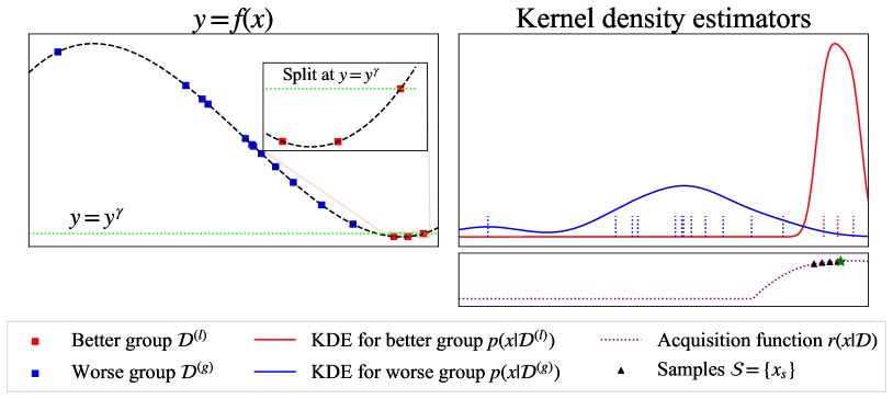
where the top-quantile $\gamma$ is computed at each iteration based on the number of observations $N(=|\mathcal{D}|)$ (see Section 3.1), and $y^{\gamma}$ is the top-$\gamma$-quantile objective value in the set of observations $\mathcal{D}$; see Figure 1 for the intuition. For simplicity, we assume that $\mathcal{D}$ is already sorted by $y_{n}$ such that $y_{1}\leq y_{2}\leq\dots\leq y_{N}$. Then the better group and the worse group are obtained as $\mathcal{D}^{(l)}=\{(\bm{x}_{n},y_{n})\}_{n=1}^{N^{(l)}}$ and $\mathcal{D}^{(g)}=\{(\bm{x}_{n},y_{n})\}_{n=N^{(l)}+1}^{N}$ where $N^{(l)}=\lceil\gamma N\rceil$. The KDEs in Eq. (6) are estimated via:

$$p(\bm{x}|\mathcal{D}^{(l)}) =w_{0}^{(l)}p_{0}(\bm{x})+\sum_{n=1}^{N^{(l)}}w_{n}k(\bm{x},\bm{x}_{n}|b^{(l)}),$$ (7)

$$p(\bm{x}|\mathcal{D}^{(g)}) =w_{0}^{(g)}p_{0}(\bm{x})+\sum_{n=N^{(l)}+1}^{N}w_{n}k(\bm{x},\bm{x}_{n}|b^{(g)})$$

where the weights $\{w_{n}\}_{n=1}^{N}$ are determined at each iteration (see Section 3.2), $k$ is a kernel function (see Section 3.3), $b^{(l)},b^{(g)}\in\mathbb{R}_{+}$ are the bandwidth (see Section 3.3.4) and $p_{0}$ is non-informative prior (see Section 3.3.5). Note that the summations of weights, i.e. $w_{0}^{(l)}+\sum_{n=1}^{N^{(l)}}w_{n},w_{0}^{(g)}+\sum_{n=N^{(l)}+1}^{N}w_{n}$, are $1$. Using the assumption in Eq. (6), we obtain the following acquisition function:

$$\mathbb{P}(y\leq y^{\gamma}|\bm{x},\mathcal{D})\stackrel{{\scriptstyle\mathrm{rank}}}{{\simeq}}r(\bm{x}|\mathcal{D})\coloneqq\frac{p(\bm{x}|\mathcal{D}^{(l)})}{p(\bm{x}|\mathcal{D}^{(g)})}.$$ (8)

We provide the intermediate process in Appendix A. The algorithm is detailed in Algorithm 1. Lines 7–16 are the main routine of TPE. In each iteration, we first calculate the algorithm parameters of TPE and then pick the configuration with the best acquisition function value based on samples from the KDE built by the better group $p(\bm{x}|\mathcal{D}^{(l)})$. Note that we can guarantee the global convergence of TPE (?) if we use the $\epsilon$-greedy algorithm in Line 14, but we stick to the greedy algorithm as we assume quite a restrictive amount of budget ($\sim 200$ evaluations) in this paper.

3 The Algorithm Details of Tree-Structured Parzen Estimator

In this section, we describe each component of TPE and we elucidate the roles of each control parameter. More specifically, we would like to highlight how each control parameter affects the trade-off between exploitation and exploration. As discussed earlier, roughly speaking, exploitation is to search near good observations and exploration is to search unseen regions. Throughout this section, (arg_name) in each section title refers to the corresponding argument’s name in Optuna and we use the default values of Optuna v3.1.0 for each visualization if not specified. Since the details of each component vary a lot by different versions, we list the difference in Table 2.

Figure 2: The optimizations of the Styblinski function by linear and sqrt. The red and blue dots show the observations till each “X evaluations”. The lower left blue shade in each figure is the optimal point and each method should find this area with as few observations as possible. Left column: the optimization using linear. It took around $500$ evaluations to first find the optimal area due to strong exploitation. Right column: the optimization using sqrt. It took less than $100$ evaluations to first find the optimal area. Although both methods did not have any observations around the optimal area at $50$ evaluations, more exploration enabled finding the optimal area.

Figure 3: The optimizations of the Styblinski function using the splitting algorithm linear with different $\beta_{1}$ (Left column: $\beta_{1}=0.05$, Center column: $\beta_{1}=0.15$, Right column: $\beta_{1}=0.25$). The blue dots show the observations till each “X evaluations”. The lower left blue shade in each figure is the optimal point and each method should find this area with as few observations as possible. We can see scattered dots (more explorative) for a small $\beta_{1}$ and concentrated dots (more exploitative) for a large $\beta_{1}$.

Figure 4: The optimizations of the Styblinski function using the splitting algorithm sqrt with different $\beta_{2}$ (Left column: $\beta_{2}=0.25$, Center column: $\beta_{2}=0.5$, Right column: $\beta_{2}=0.75$). The red dots show the observations till each “X evaluations”. The lower left blue shade in each figure is the optimal point and each method should find this area with as few observations as possible. We can see scattered dots (more explorative) for a small $\beta_{2}$ and concentrated dots (more exploitative) for a large $\beta_{2}$.

3.1 Splitting Algorithm (gamma)

The quantile $\gamma$ is used to split $\mathcal{D}$ into the better group $\mathcal{D}^{(l)}$ and the worse group $\mathcal{D}^{(g)}$ using a function $\Gamma(N)$. The first paper (?) and the second paper (?) use the following different $\Gamma$:

1. (linear) $\gamma\coloneqq\Gamma(N)=\beta_{1}\in(0,1]$,

2. (Square root (sqrt)) $\gamma\coloneqq\Gamma(N)=\beta_{2}/\sqrt{N},\beta_{2}\in(0,\sqrt{N}]$.

The parameters used in each paper were $\beta_{1}=0.15$ and $\beta_{2}=0.25$ and they limited the number of observations in the better group $\mathcal{D}^{(l)}$ to $25$.

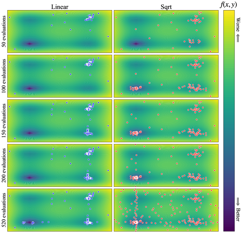
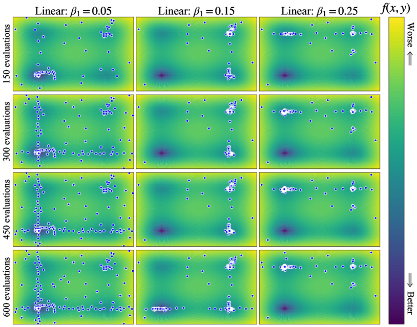
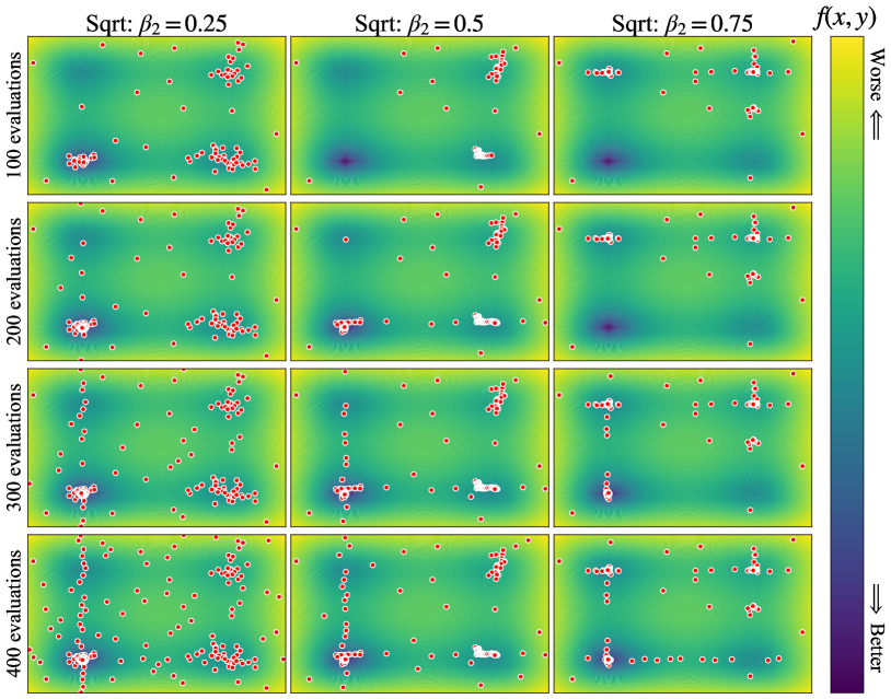
Figure 2 shows that sqrt promotes more exploration and suppresses exploitation, and Figures 3, 4 demonstrate that smaller $\beta_{1}$ and $\beta_{2}$ lead to more exploration and less exploitation. This happens because:

1. $p(\bm{x}|\mathcal{D}^{(l)})$ would have a narrower modal that requires few observations for $p(\bm{x}|\mathcal{D}^{(g)})$ to cancel out the contribution from $p(\bm{x}|\mathcal{D}^{(l)})$ in the density ratio $r(\bm{x}|\mathcal{D})$, and thus it takes less time to switch to exploration, and

2. $w_{0}^{(l)}$ occupies a larger ratio in $p(\bm{x}|\mathcal{D}^{(l)})$ in Eq. (7) due to a smaller number of observations in the better group $\mathcal{D}^{(l)}$ and it promotes exploration.

On the other hand, when the objective function has multiple modals, the multi-modality in $p(\bm{x}|\mathcal{D}^{(l)})$ allows to explore all modalities, and large $\beta_{1}$ or $\beta_{2}$ does not necessarily lead to poor performance. It explains why ? (?, ?) used linear, which gives a larger $\gamma$, for multi-objective settings.

Figure 5: The distributions of each weighting algorithm when using $N^{(g)}=100$. Left: the weight distribution for the uniform. Right: the weight distribution for the old decay. Older observations get lower weights and the latest 25 observations get the uniform weight.

Table 1: The advantages and disadvantages of each weighting algorithm.

Weighting algorithm Advantages Disadvantages Uniform - Use all observations equally - Take time to account the recent observations - Not need careful preprocessing of $y$ - Not consider the ranking in each group Old decay - Take less time to switch to exploration - Might waste the knowledge from the past - Not need careful preprocessing of $y$ - Not consider the ranking in each group Expected improvement - Consier the ranking in the better group - Need careful preprocessing of $y$

3.2 Weighting Algorithm (weights, prior_weight)

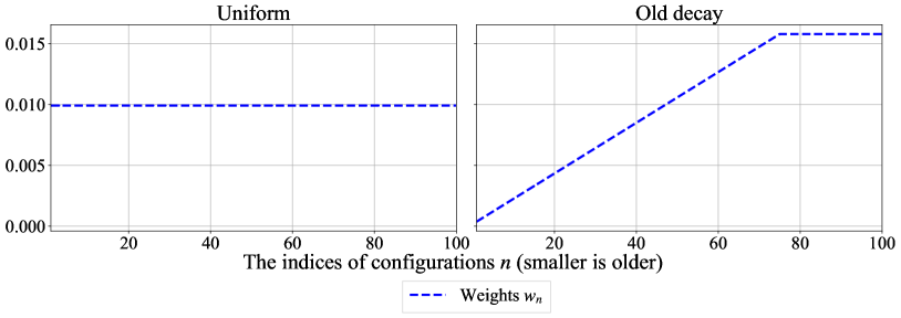
The weighting algorithm $W$ is used to determine the weights $\{w_{n}\}_{n=1}^{N}$ for KDEs. For simplicity, we denote the prior weights as $w_{0}^{(l)}\coloneqq w_{0}$ and $w_{0}^{(g)}\coloneqq w_{N+1}$, and we consider only prior_weight=1.0, which is the default value; see Section 3.3.5 for more details about prior_weight. The first paper (?) uses the following uniform weighting algorithm:

$$w_{n}\coloneqq\left\{\begin{array}[]{ll}\frac{1}{N^{(l)}+1}&(n=0,\dots,N^{(l)})\\ \frac{1}{N^{(g)}+1}&(n=N^{(l)}+1,\dots,N+1)\end{array}\right.,$$ (11)

In contrast, the second paper (?) uses the following old decay weighting algorithm:

$$w_{n}\coloneqq\left\{\begin{array}[]{ll}\frac{1}{N^{(l)}+1}&(n=0,\dots,N^{(l)})\\ \frac{w_{n}^{\prime}}{\sum_{n=N^{(l)}+1}^{N+1}w_{n}^{\prime}}&(n=N^{(l)}+1,\dots,N+1)\end{array}\right..$$ (14)

where $w_{n}^{\prime}$ (for $n=N^{(l)}+1,\dots,N+1$) is defined as:

$$w_{n}^{\prime}\coloneqq\left\{\begin{array}[]{ll}1&(t_{n}>N^{(g)}+1-T_{\mathrm{old}})\\ \tau(t_{n})+\frac{1-\tau(t_{n})}{N^{(g)}+1}&(\mathrm{otherwise})\end{array}\right..$$ (17)

Note that $t_{n}\in\{1,\dots,N^{(g)}+1\}$ for $n=N^{(l)}+1,\dots,N+1$ is the query order, which means $t_{n}=1$ is the oldest and $t_{n}=N^{(g)}+1$ is the youngest, of the $n$-th observation in $\mathcal{D}^{(g)}$, and the decay rate is $\tau(t_{n})\coloneqq(t_{n}-1)/(N^{(g)}-T_{\mathrm{old}})$ where $T_{\mathrm{old}}=25$ in the original paper (?). We take $t_{N+1}=1$ to view the prior as the oldest information. We visualize the weight distribution in Figure 5. The old decay aims to assign smaller weights to older observations as the search should focus on the current region of interest and should not be distracted by the earlier regions of interest. Furthermore, the following computation makes the acquisition function expected improvement (EI) more strictly (?):

$$w_{n}\coloneqq\left\{\begin{array}[]{ll}\frac{y^{\gamma}-y_{n}}{\sum_{n=1}^{N^{(l)}}(1+1/N^{(l)})(y^{\gamma}-y_{n})}&(n=1,\dots,N^{(l)})\\ \frac{1}{N^{(g)}+1}&(n=N^{(l)}+1,\dots,N+1)\\ \end{array}\right.$$ (20)

where $w^{\prime}_{0}$ is the mean of $y^{\gamma}-y_{n}$ for $n=1,\dots,N^{(l)}$ and

$$w_{0}\coloneqq\frac{\sum_{n=1}^{N^{(l)}}(y^{\gamma}-y_{n})/N^{(l)}}{\sum_{n=1}^{N^{(l)}}(1+1/N^{(l)})(y^{\gamma}-y_{n})}.$$ (21)

Note that the weighting algorithm used in MOTPE (?) was proven to be EI by ? (?) although it was not explicitly mentioned in the MOTPE paper.

In Table 1, we list the advantages and disadvantages of each weighting algorithm. While EI can consider the scale of $y$, we need to carefully preprocess $y$ (e.g. standardization and log transformation). For uniform and old decay, while it might be probably better to use old decay with an abundant computational budget, it is recommended to perform multiple independent TPE runs in such cases.

3.3 Kernel Functions

The kernel function is used to build the surrogate model in TPE. For the discussion of the kernel function, we consistently use the notation $k_{d}:\mathcal{X}_{d}\times\mathcal{X}_{d}\rightarrow\mathbb{R}_{\geq 0}$ to refer to the kernel function in the $d$-th dimension and focus on the uniform weight for simplicity.

3.3.1 Kernel for Numerical Parameters

For numerical parameters, we consistently use the following Gaussian kernel:

$$g(x,x_{n}|b)\coloneqq\frac{1}{\sqrt{2\pi b^{2}}}\exp{\biggl{[}-\frac{1}{2}\biggl{(}\frac{x-x_{n}}{b}\biggr{)}^{2}\biggr{]}}$$ (22)

In the original paper, the authors employed the truncated Gaussian kernel $k_{d}(x,x_{n})\coloneqq g(x,x_{n}|b)/Z(x_{n})$ where $Z(x_{n})\coloneqq\int_{L}^{R}g(x,x_{n}|b)dx$ is a normalization constant and the domain of $x$ is $\mathcal{X}_{d}\coloneqq[L,R]$. The parameter $b\in\mathbb{R}_{+}$ in the Gaussian kernel is called bandwidth, and ? (?) used Scott’s rule (?) (see Appendix C.3.2) and ? (?) used a heuristic to determine the bandwidth $b$ as described in Appendix C.3.1. In this paper, we use Scott’s rule as a main algorithm to be consistent with the classical KDE basis. Note that for a discrete parameter $x\in\{L,L+q,\dots,R\}$, the kernel is computed as:

$$k_{d}(x,x_{n})\coloneqq\frac{1}{Z(x_{n})}\int_{x-q/2}^{x+q/2}g(x^{\prime},x_{n}|b)dx^{\prime}$$ (23)

where we defined $R\coloneqq L+(K-1)q$, $q\in\mathbb{R}$, and $K\in\mathbb{Z}_{+}$. The normalization constant for the discrete kernel is computed as $Z(x_{n})\coloneqq\int_{L-q/2}^{R+q/2}g(x^{\prime},x_{n}|b)dx^{\prime}$. A large bandwidth leads to more exploration and a small bandwidth leads to less exploration as discussed in Section 3.3.4.

3.3.2 Kernel for Categorical Parameters

For categorical parameters, we consistently use the following Aitchison-Aitken kernel (?):

$$k_{d}(x,x_{n}|b)=\left\{\begin{array}[]{ll}1-b&(x=x_{n})\\ \frac{b}{C-1}&(\mathrm{otherwise})\end{array}\right.$$ (26)

where $C$ is the number of choices in the categorical parameter and $b\in[0,1)$ is the bandwidth for this kernel. Note that Optuna v3.1.0 uses a heuristic shown in Appendix C.3 to compute the bandwidth $b$ and we refer to this heuristic as optuna in the ablation study. The bandwidth in this kernel also controls the degree of exploration and a large bandwidth leads to more exploration.

Figure 6: The difference between KDEs by univariate and multivariate kernels. The brighter color shows high density. Left: the contour plot of the KDE by the univariate kernel. As the univariate kernel cannot capture the interaction effects, we see bright colors even at the top-left and bottom-right regions. Right: the contour plot of the KDE by the multivariate kernel. As the multivariate kernel can capture the interaction effects, we see bright colors only near the observations.

Figure 7: The optimizations of the Sphere function using the multivariate and univariate kernels. The red and blue dots show the observations till each “X evaluations”. The blue shade in each figure is the optimal point and each method should find this area with as less observations as possible. Left column: the optimization using the multivariate kernel. Exploration starts after the center part is covered. Right column: the optimization using the univariate kernel. The observations gather close to the two lines $x_{1}=0$ and $x_{2}=0$ because the univariate kernel cannot account for interaction effects.

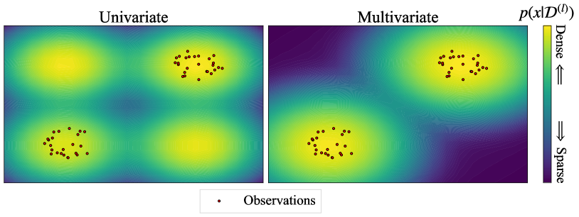
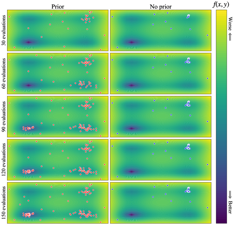
3.3.3 Univariate Kernel vs Multivariate Kernel (multivariate)

In the original paper (?, ?), the authors used the so-called univariate KDEs:

$$p(\bm{x}|\{\bm{x}_{n}\}_{n=1}^{N})\coloneqq\frac{1}{N}\prod_{d=1}^{D}\sum_{n=1}^{N}k_{d}(x_{d},x_{n,d}|b)$$ (27)

where $x_{n,d}\in\mathcal{X}_{d}$ is the $d$-th dimension of the $n$-th observation $\bm{x}_{n}$. ? (?, ?) used the univariate kernel to handle the tree-structured search space, a.k.a. a search space with some conditional parameters. The univariate kernel can handle conditional parameters because of the independence of each dimension. On the other hand, ? (?) used the following multivariate KDEs to enhance the performance in exchange for the conditional parameter handling:

$$p(\bm{x}|\{\bm{x}_{n}\}_{n=1}^{N})\coloneqq\frac{1}{N}\sum_{n=1}^{N}\prod_{d=1}^{D}k_{d}(x_{d},x_{n,d}|b).$$ (28)

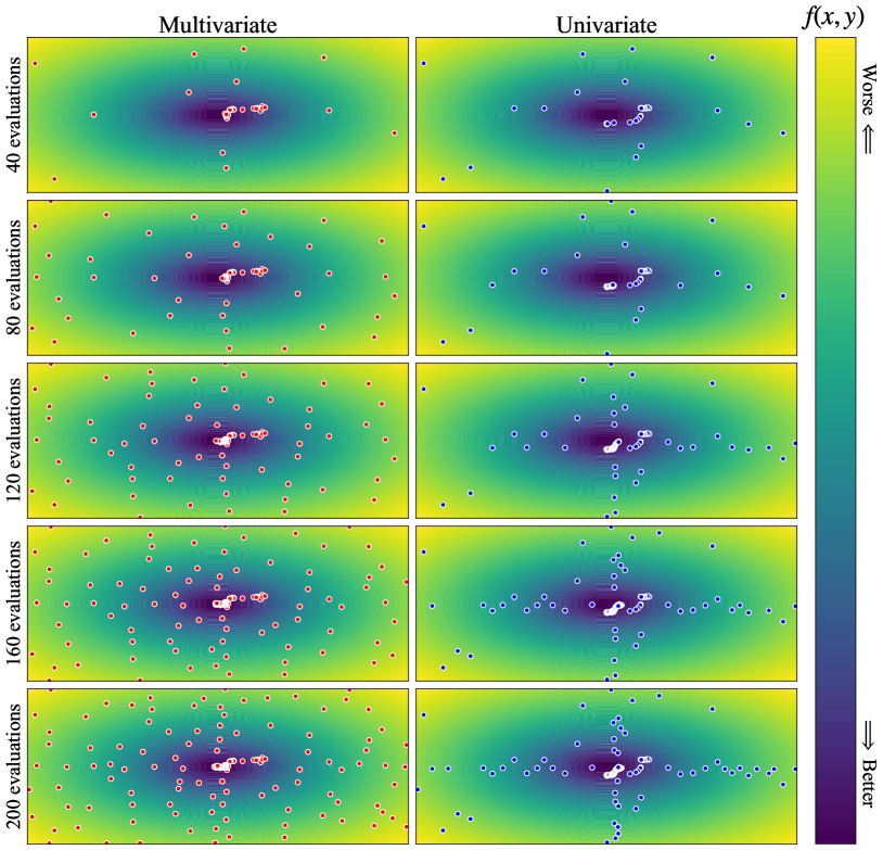
Note that when we set group=True, which we explain in Appendix C.2, in Optuna, the multivariate kernel can also be applied to the tree-structured search space. As mentioned earlier, the multivariate kernel is important to improve the performance. According to Eq. (27), since $\sum_{n=1}^{N}k_{d}(x_{d},x_{n,d}|b)$ is independent  of that of another dimension $d^{\prime}(\neq d)$, the optimization of each dimension can be separately performed and it cannot capture the interaction effect as seen in Figure 6. In contrast, as the multivariate kernel considers interaction effects, it is unlikely to be misguided compared to the univariate kernel. In fact, while the multivariate kernel recognized the exact location of the modal in Figure 7, TPE with the univariate kernel ended up searching the axes $x_{1}=0$ and $x_{2}=0$ separately because it does not have the capability to recognize the exact location of the modal. Although the separate search of each dimension is disadvantageous for many cases, it was effective for objective functions with many modals such as the Xin-She-Yang function and the Rastrigin function.

3.3.4 Bandwidth Modification (consider_magic_clip)

Figure 8: The change in the density ratio $r(\bm{x}|\mathcal{D})$ (purple dotted lines in Bottom row) with respect to the minimum bandwidth $b_{\min}$. Both settings use the same observations (red and blue dotted lines in Top row). Left: a small $b_{\min}$. Since the KDE for the better group (red line) has a sharp peak, the density ratio is sharply peaked. Right: a large $b_{\min}$. The density ratio is horizontally distributed.

Figure 9: A concrete example where the minimum bandwidth matters. The black dashed lines are the true objective function without noise and the red dots are the observations with noise. Left: a function that has a large noise compared to the variation with respect to $x$. As can be seen, some observations near $x=1$ are better than some observations near $x=1$ due to the noise. In such cases, smaller $b_{\min}$, which leads to more precise optimizations, does not make much difference. Right: a function that has a small noise compared to the variation with respect to $x$. Since the noise is small, smaller $b_{\min}$ helps to yield precise solutions.

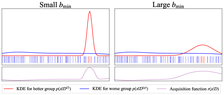
For the bandwidth of the numerical kernel defined on $[L,R]$, we first compute the bandwidth $b$ by a heuristic, e.g. Scott’s rule (?), and then we modify the bandwidth $b$ by the so-called magic clipping. Note that the heuristics of bandwidth selection used in TPE are discussed in Appendix C.3. ? (?) applied the magic clipping as follows:

$$b_{\mathrm{new}}\coloneqq\max(\{b,b_{\min}\})~{}\mathrm{where}~{}b_{\min}\coloneqq\frac{R-L}{\min(\{100,N\})}$$ (29)

and we input $N=N^{(l)}+1$ for $p(\bm{x}|\mathcal{D}^{(l)})$ and $N^{(g)}+1$ for $p(\bm{x}|\mathcal{D}^{(g)})$. Note that if $p(\bm{x}|\mathcal{D}^{(\cdot)})$ does not include the prior $p_{0}$, we input $N=N^{(\cdot)}$ instead. In principle, a small $b_{\min}$ leads to stronger exploitation and a large $b_{\min}$ leads to stronger exploration as can be seen in Figure 8. Mostly, the modification by the magic clipping expands the bandwidth and it changes the degree of how precisely we should search each parameter. For example, when we search for the best dropout rate of neural networks from the range of $[0,1]$, we might want to distinguish the difference between $0.4$ and $0.5$, but we maybe do not need to differentiate between $0.4$ and $0.41$ because it is likely that the performance variation is caused by noise.

To illustrate what we mean, Figure 9 shows objective functions with different noise levels. When the noise is dominant compared to the variation caused by a parameter (Left), a small bandwidth, which allows to precisely optimize, is not necessary. On the other hand, when the noise is negligible (Right), a small bandwidth is necessary. While it is probably better to precisely optimize the parameter for the small noise case, we might want to pick a value from $\{-5,-4,\dots,4,5\}$ for the noisy case. We call the size of such an intrinsic set of values intrinsic cardinality, which is $\mathrm{card}(\{-5,-4,\dots,4,5\})=11$ in this example. The scale of $b_{\min}$ should be inversely proportional to the intrinsic cardinality of each parameter. Since the appropriate setting of $b_{\min}$ is very important for efficient optimization and strong performance, we individually analyze the bandwidth modification in the ablation study.

Figure 10: The optimizations of the Styblinski function with and without prior $p_{0}$. The red and blue dots show the observations till each “X evaluations”. The lower left blue shade in each figure is the optimal point and each method should find this area with as less observations as possible. Left column: the optimization with prior. Unseen regions were explored every time each modal is covered by many observations. Right column: the optimization without prior. No exploration happened after one of the modals were found.

3.3.5 Non-Informative Prior (consider_prior, prior_weight)

Prior is $p_{0}$ in Eq. (7). For numerical parameters defined on $[L,R]$, $p_{0}$ is the PDF of Gaussian distribution $\mathcal{N}((R+L)/2,(R-L)^{2})$, and for categorical parameters $\{1,\dots,C\}$, $p_{0}$ is the probability mass function of uniform categorical distribution $\mathcal{U}(\{1,\dots,C\})$. Since $N^{(l)}$ is usually very small throughout an optimization, the prior is especially important for $p(\bm{x}|\mathcal{D}^{(l)})$ and it prevents strong exploitation as seen in Figure 10. prior_weight amplifies the contribution from the prior. As discussed later, the prior is indispensable to TPE. For example, when we set prior_weight=2.0, the weights $w^{(l)}_{0},w^{(g)}_{0}$ will be doubled. Therefore, a large prior_weight promotes exploration.

Table 2: The differences in each component of different versions of TPE. Other components such as prior and the number of initial configurations are shared across different versions. TPE (2011), TPE (2013), BOHB, MOTPE, c-TPE, and Optuna refer to TPE by ? (?), TPE (Hyperopt) by ? (?), TPE in BOHB (?), TPE in MOTPE (?), TPE in c-TPE (?), and TPE in Optuna v3.1.0, respectively. Note that uniform of BOHB is computed by Eq. (33), and c-TPE uses a fixed $b_{\min}$ instead of magic clipping. For the bandwidth selection, hyperopt, scott, and optuna refer to Eqs. (37), (38), and (39) in Appendix C.3, respectively. BOHB calculates the bandwidth of categorical parameters using scott as if they are numerical parameters.

Version Splitting Weighting Bandwidth Multivariate Magic clipping (gamma) (weights) Numerical Categorical (multivariate) (consider_magic_clip) TPE (2011) linear, $\beta_{1}=0.15$ uniform hyperopt $b=0$ False True TPE (2013) sqrt, $\beta_{2}=0.25$ old decay hyperopt $b=0$ False True BOHB linear, $\beta_{1}=0.15$ uniform^⋆ scott scott True False MOTPE linear, $\beta_{1}=0.10$ EI hyperopt $b=0$ False True c-TPE sqrt, $\beta_{2}=0.25$ uniform scott $b=0.2$ True False^⋆ Optuna linear, $\beta_{1}=0.10$ old decay optuna Eq. (40) True True

4 Experiments

Table 3: The search space of the control parameters used in the ablation study. Note that $\beta_{1},\beta_{2}$ are conditional parameters and we have $2\times 2\times 2\times(4+4)\times 4\times 4=1024$ possible combinations in total.

Component	Choices
Multivariate (multivariate)	{True, False}
Use prior $p_{0}$ (consider_prior)	{True, False}
Use magic clipping (consider_magic_clip)	{True, False}
Splitting algorithm $\Gamma$ (gamma)	{linear, sqrt}
1. $\beta_{1}$ in linear	{0.05, 0.10, 0.15, 0.20}
2. $\beta_{2}$ in sqrt	{0.25, 0.50, 0.75, 1.0}
Weighting algorithm $W$ (weights)	{uniform, old-decay, old-drop, EI}
Categorical bandwidth $b$ in Eq. (26)	{0.8, 0.9, 1.0, optuna}

In this section, we first provide the ablation study of each control parameter and present the recommendation of the default values. Then, we further investigate the enhancement for bandwidth selection. Finally, we compare the enhanced TPE with various baseline methods.

4.1 Ablation Study

In this experiment, we identify the importance of each control parameter discussed in the previous section via the ablation study and provide the recommended default setting.

4.1.1 Setup

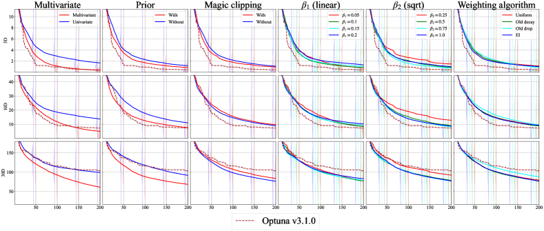
The goal of the ablation study is to identify good sets of default values from the search space specified in Table 3 and analyze the results. Note that we added old-drop, which gives uniform weights to the recent $T_{\mathrm{old}}=25$ observations and drops the weights (i.e. to give zero weights) for the rest, to the choices of the weighting algorithm to identify whether old information is necessary for optimizations. For the other parameters not specified in the table, we fixed them to the default values of Optuna v3.1.0 except we used Scott’s rule in Eq. (38) for the numerical bandwidth selection. To strengthen the reliability of the analysis, we took a diverse set of $51$ objective functions listed in Appendix D. The objective functions include $36$ benchmark functions ($12$ different functions $\times$ $3$ different dimensionalities), $8$ tasks in HPOBench (?), $4$ tasks in HPOlib (?), and $3$ tasks in JAHS-Bench-201 (?). For EI, we used the default scale of $y$ except on HPOlib which we used the log scale of the validation MSE. Each objective function is optimized using $10$ different seeds and each optimization observes $200$ configurations. For the initialization, we followed the default setting of Optuna v3.1.0 and initialized each optimization with $10$ random configurations (i.e. n_startup_trials=10).

We explain the methodologies, which are based on ? (?), for our analysis. Assume that there are $K$ possible combinations of control parameters and we obtain a set of observations $\{(\bm{x}_{k,n}^{(m)},y_{k,n}^{(m)})\}_{n=1}^{N}$ on the $m$-th benchmark ($m=1,\dots,M$) with the $k$-th possible set of the control parameters $\bm{\theta}_{k}$ where $\bm{\theta}_{k}$ ($k=1,\dots,K$) is one of the possible sets of the control parameters specified in Table 3 and we use $N=200$ in the experiments. Then we collect a set of results $\mathcal{R}_{n}^{(m)}\coloneqq\{(\bm{\theta}_{k},\zeta^{(m)}_{k,n})\}_{k=1}^{K}$ with the budget of $n$ where $\zeta_{k,n}^{(m)}\coloneqq\min_{n^{\prime}\leq n}y_{k,n^{\prime}}^{(m)}$ and we used $n\in\{50,100,150,200\}$ in the experiments. Furthermore, we define $i_{m,k}$ ($k=1,\dots,K$) so that $\zeta^{(m)}_{i_{m,1},n}\leq\zeta^{(m)}_{i_{m,2},n}\leq\dots\leq\zeta^{(m)}_{i_{m,K},n}$. For the visualization of the probability mass functions, we performed the following operations:

1. Pick a top-performance quantile $\alpha$ (in our case, $\alpha=0.05,0.5$),

2. Extract the top-$\alpha$ quantile observations $\{(\bm{\theta}_{i_{m,k}},\zeta^{(m)}_{i_{m,k},n})\}_{k=1}^{\lceil\alpha K\rceil}$,

3. Build 1D KDEs $p_{d}^{(m)}(\theta_{d})\coloneqq\sum_{k=1}^{\lceil\alpha N\rceil}k(\theta_{d},\theta_{i_{m,k},d})$ for each control parameter,

4. Take the mean of the KDEs from all the tasks $\bar{p}_{d}\coloneqq 1/M\sum_{m=1}^{M}p_{d}^{(m)}(\theta_{d})$,

5. Plot the probability mass function of the mean $\bar{p}_{d}$ of the KDEs.

For the hyperparameter importance (HPI), we used PED-ANOVA (?) and compute the HPI to achieve the top-$50\%$ performance (global HPI) and to achieve the top-$5\%$ performance from the top-$50\%$ performance (local HPI).

(a) Benchmark functions with 5D

(b) Benchmark functions with 10D

(c) Benchmark functions with 30D

Figure 11: The probability mass values of each control parameter in the top-$5\%$ and top-$50\%$ observations at {50,100,150,200} evaluations on the benchmark functions. High probability mass in a specific value implies that we are likely to yield top-$5\%$ or top-$50\%$ performance with the specific value.

Table 4: The hyperparameter importance (HPI) of each control parameter on the benchmark functions to achieve top $50\%$ and to improve to top $5\%$ from top $50\%$. HPI is measured at {50, 100, 150, 200} evaluations. We bolded the top-2 HPI. Note that while the HPI in $\beta$ quantifies whether variating $\beta$ given either linear or sqrt matters, that in “Splitting algorithm” quantifies whether switching between linear and sqrt matters.

Dimension Control parameter The number of function evaluations 50 evaluations 100 evaluations 150 evaluations 200 evaluations Top $50\%$ Top $5\%$ Top $50\%$ Top $5\%$ Top $50\%$ Top $5\%$ Top $50\%$ Top $5\%$ 5D Multivariate 23.67% 12.77% 41.39% 14.71% 48.67% 10.90% 50.81% 11.28% Prior 6.21% 9.45% 4.65% 10.47% 6.57% 8.87% 8.45% 10.19% Magic clipping 36.11% 10.35% 21.65% 9.33% 15.19% 8.77% 10.45% 12.60% Splitting algorithm 1.09% 0.97% 1.78% 3.33% 1.95% 2.95% 3.05% 3.09%       $\beta_{1}$ (linear) 9.80% 17.95% 7.10% 11.04% 5.80% 8.37% 7.24% 16.86%       $\beta_{2}$ (sqrt) 19.24% 39.12% 20.80% 27.89% 17.64% 39.32% 16.08% 22.36% Weighting algorithm 3.87% 9.39% 2.62% 23.22% 4.18% 20.82% 3.92% 23.62% 10D Multivariate 8.39% 16.64% 26.23% 14.87% 44.48% 14.38% 48.94% 14.24% Prior 25.69% 11.48% 12.96% 14.76% 6.31% 18.81% 4.50% 19.72% Magic clipping 38.79% 20.09% 31.63% 14.98% 25.45% 14.60% 21.81% 11.44% Splitting algorithm 0.87% 0.69% 2.34% 2.23% 3.32% 2.48% 3.76% 3.23%       $\beta_{1}$ (linear) 7.83% 20.42% 8.49% 17.92% 5.77% 15.04% 5.68% 13.81%       $\beta_{2}$ (sqrt) 14.70% 24.06% 15.79% 22.84% 11.83% 21.78% 11.51% 25.76% Weighting algorithm 3.74% 6.61% 2.55% 12.41% 2.84% 12.91% 3.78% 11.81% 30D Multivariate 32.83% 17.15% 18.62% 18.37% 31.01% 16.89% 36.80% 15.23% Prior 29.53% 14.52% 24.91% 15.55% 12.38% 19.74% 9.52% 20.66% Magic clipping 16.31% 26.46% 31.82% 18.99% 28.84% 14.69% 27.98% 12.38% Splitting algorithm 1.06% 1.87% 2.12% 3.17% 1.58% 5.57% 2.45% 5.69%       $\beta_{1}$ (linear) 4.82% 17.80% 4.54% 23.22% 8.66% 22.77% 6.26% 22.58%       $\beta_{2}$ (sqrt) 12.17% 8.56% 11.24% 8.94% 8.56% 7.93% 9.86% 8.71% Weighting algorithm 3.28% 13.65% 6.75% 11.75% 8.96% 12.40% 7.13% 14.75%

(a) HPOBench

(b) HPOlib

(c) JAHS-Bench-201

Figure 12: The probability mass values of each control parameter in the top-$5\%$ and top-$50\%$ observations at {50,100,150,200} evaluations on the HPO benchmarks. High probability mass in a specific value implies that we are likely to yield top-$5\%$ or top-$50\%$ performance with the specific value.

Table 5: The hyperparameter importance (HPI) of each control parameter on the HPO benchmarks to achieve top $50\%$ and to improve to top $5\%$ from top $50\%$. HPI is measured at {50, 100, 150, 200} evaluations. We bolded the top-2 HPI. Note that while the HPI in $\beta$ quantifies whether variating $\beta$ given either linear or sqrt matters, that in “Splitting algorithm” quantifies whether switching between linear and sqrt matters.

Benchmark Control parameter The number of function evaluations 50 evaluations 100 evaluations 150 evaluations 200 evaluations Top $50\%$ Top $5\%$ Top $50\%$ Top $5\%$ Top $50\%$ Top $5\%$ Top $50\%$ Top $5\%$ HPOBench Multivariate 1.41% 6.79% 2.99% 8.35% 3.29% 4.78% 5.11% 6.36% Prior 15.43% 0.60% 11.11% 1.95% 11.78% 2.90% 10.93% 3.30% Magic clipping 38.76% 10.16% 63.38% 11.95% 60.96% 12.77% 62.16% 12.43% Splitting algorithm 2.00% 7.61% 1.29% 12.26% 1.11% 4.44% 1.02% 2.98%       $\beta_{1}$ (linear) 12.61% 37.74% 3.12% 29.52% 6.00% 36.62% 7.94% 42.21%       $\beta_{2}$ (sqrt) 27.87% 29.51% 17.18% 28.03% 15.49% 23.06% 10.87% 15.18% Weighting algorithm 1.93% 7.59% 0.93% 7.94% 1.38% 15.43% 1.97% 17.53% HPOlib Multivariate 3.06% 20.88% 15.51% 16.10% 19.25% 17.85% 21.00% 17.09% Prior 8.88% 6.11% 23.51% 7.56% 31.62% 10.95% 35.41% 10.44% Magic clipping 72.53% 5.89% 38.75% 10.62% 28.31% 13.90% 22.96% 16.06% Splitting algorithm 0.30% 0.51% 0.53% 0.20% 1.51% 0.30% 2.52% 0.80%       $\beta_{1}$ (linear) 6.32% 28.93% 7.62% 17.43% 6.33% 15.05% 6.58% 19.45%       $\beta_{2}$ (sqrt) 6.70% 26.03% 4.92% 29.81% 2.34% 26.18% 0.97% 19.84% Weighting algorithm 1.98% 4.91% 7.99% 9.79% 8.92% 8.40% 8.36% 8.23% Categorical bandwidth: $b$ 0.23% 6.73% 1.16% 8.50% 1.72% 7.37% 2.20% 8.08% JAHS-Bench-201 Multivariate 11.47% 20.27% 16.16% 23.69% 17.05% 20.26% 19.79% 16.73% Prior 33.05% 5.63% 38.34% 8.17% 40.41% 8.09% 41.88% 7.62% Magic clipping 19.53% 3.75% 13.59% 5.26% 12.29% 9.45% 11.90% 11.42% Splitting algorithm 1.16% 1.22% 0.94% 3.98% 1.45% 6.03% 1.52% 5.28%       $\beta_{1}$ (linear) 3.24% 34.47% 1.34% 12.62% 2.68% 10.23% 2.94% 11.18%       $\beta_{2}$ (sqrt) 12.84% 20.15% 10.78% 28.97% 8.81% 25.91% 5.29% 28.18% Weighting algorithm 5.80% 5.28% 10.22% 11.52% 9.89% 12.87% 10.38% 12.66% Categorical bandwidth: $b$ 12.91% 9.22% 8.62% 5.79% 7.41% 7.16% 6.30% 6.93%

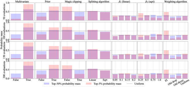
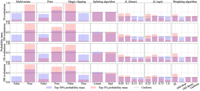
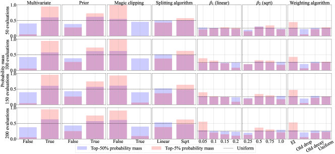
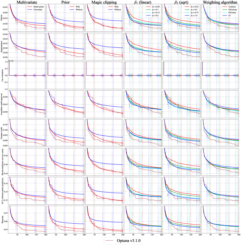
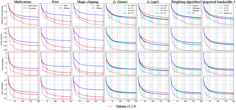
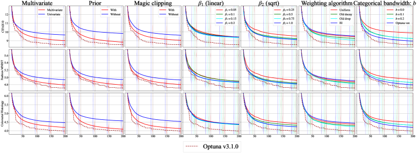
4.1.2 Results & Discussion

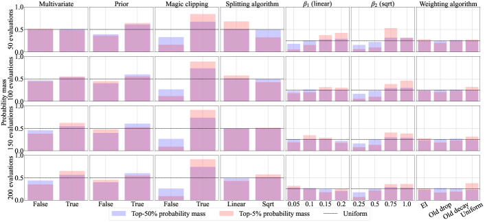
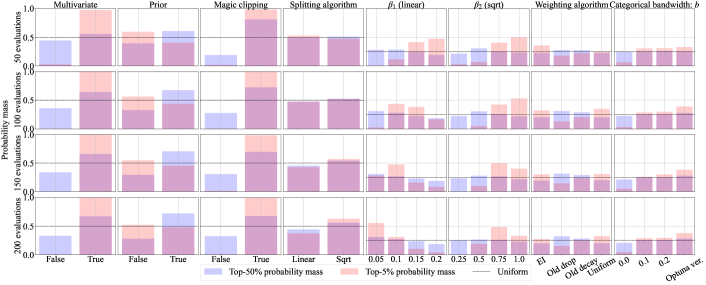
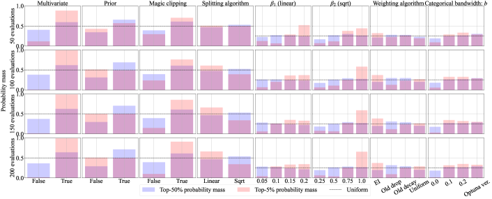
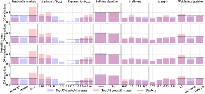
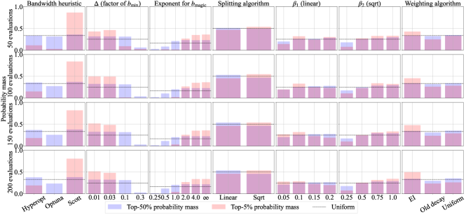
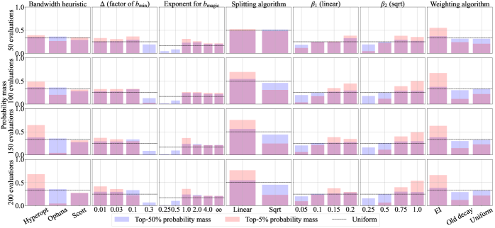
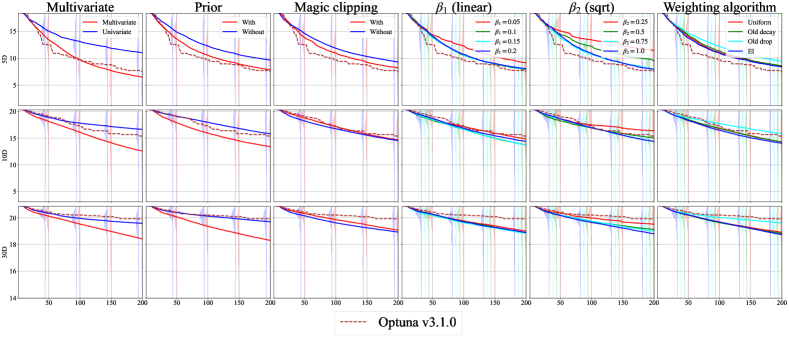
Figures 11,12 present the probability mass of each choice in the top-$50\%$ and -$5\%$ observations and Tables 4,5 present the HPI of each control parameter. Note that since the analysis loses some detailed information, we provided individual results and the details of the analysis in Appendix E.

Multivariate (multivariate): the settings with the multivariate kernel yielded a strong peak in the top-$5\%$ probability mass for almost all settings and the mean performance in the individual results showed that the multivariate kernel outperformed the univariate kernel except on the 10- and 30-dimensional Xin-She-Yang function. For the benchmark functions, the multivariate kernel is one of the most dominant factors and the HPI went up as the number of evaluations increases in the low-dimensional problems. It matches the intuition that the multivariate kernel needs more observations to be able to exploit useful information. Although the multivariate kernel was not essential for HPOBench, it is recommended to use the multivariate kernel.

Prior (consider_prior): while the settings with the prior $p_{0}$ yielded a strong peak in the top-$50\%$ probability mass for all the settings, it was not the case in the top-$5\%$ probability mass for the HPO benchmarks. For HPOBench and JAHS-Bench-201, although the settings with the prior were more likely to achieve the top-$5\%$ performance in the early stage of optimizations, the likelihood decreased over time. It implies that the prior (more exploration) is more effective in the beginning. On the other hand, for HPOlib, the likelihood of achieving the top-$5\%$ performance was higher in the settings without the prior. It implies that we should reduce the prior (more exploitation) in the beginning for HPOlib. According to the individual results, while the performance distributions of the settings without the prior were close to uniform, those with the prior has a stronger modal. It means that the prior was primarily important for the top-$50\%$ as can be seen in Tables 4,5 as well and the settings without the prior require more careful tuning. Although some settings on HPOlib without the prior could outperform those with the prior, we recommend using the prior because the likelihood difference is not striking.

Magic clipping (consider_magic_clip): according to the probability mass, the magic clipping has a negative impact on the benchmark functions and a positive impact on the HPO benchmarks. Almost no settings could achieve the top-$5\%$ performance with the magic clipping for the high-dimensional benchmark functions. The results relate to the noise level and the intrinsic cardinality discussed in Section 3.3.4. Since the magic clipping affects the performance strongly, we will investigate more in the next section.

Splitting algorithm and $\beta$ (gamma): the choice of either linear or sqrt does not affect strongly achieving the top-$50\%$. Although the HPI of the splitting algorithm is dominated by the other HPs, the splitting algorithm choice slightly affected the results. For example, while linear was more effective for the 5D benchmark functions, sqrt was more effective for the 30D benchmark functions. Since linear promotes exploitation and sqrt promotes exploration as discussed in Section 3.1, it might be useful to change the splitting algorithm depending on the dimensionality of the search space. However, the choice of $\beta$ was much more important according to the tables and we, unfortunately, could not see similar patterns in each figure although we got the following findings:

• peaks of $\beta_{1}$ in linear largely changed over time,

• peaks of $\beta_{2}$ in sqrt did not change a lot,

• the peaks change from larger $\beta$ to small $\beta$ over time (exploitation to exploration),

• linear with a small $\beta_{1}$ was effective for the high-dimensional benchmark functions,

• sqrt with a large $\beta_{2}$ was effective for the HPO benchmarks,

Another finding is that while we see that the benchmark functions required more exploitation and the HPO benchmarks required more exploration from the magic clipping, the benchmark functions tended to require more exploration from a small $\beta$ and the HPO benchmarks tended to require more exploitation from a large $\beta$. It implies that each component controls the trade-off between exploration and exploitation differently and we need to carefully tune each control parameter. However, linear with $\beta_{1}=0.1$ and sqrt with $\beta_{2}=0.75$ exhibited relatively stable performance for each problem.

Weighting algorithm (weights): although the weighting algorithm was not an important factor to attain the top-$50\%$ performance, the results showed that EI was effective to attain the top-$5\%$ performance, and uniform came next. Note that since the behavior of EI heavily depends on the distribution of the objective value $p(y)$, EI might require special treatment on $y$ as in the scale of HPOlib. For example, when the objective can take infinity, we cannot really define the weights in Eq. (20). According to the top-$50\%$ probability mass of the HPO benchmarks, old-decay and old-drop were the most frequent choices. It implies that while they are relatively robust to the choice of other control parameters, the regularization effect caused by dropping past observations limits the performance.

Categorical bandwidth $b$: for the categorical bandwidth, we found out that it is hard to attain the top-$5\%$ performance with $b=0$ because it tends to cause overfitting to one category. Otherwise, any choices exhibited more or less similar performance and optuna yielded slightly better performance than other choices.

To sum up the results of the ablation study, our recommendation is to use:

• multivariate=True,

• consider_prior=True,

• consider_magic_clip=True for the HPO benchmarks and False for the benchmark functions,

• gamma=linear with $\beta_{1}=0.1$ or gamma=sqrt with $\beta_{2}=0.75$,

• weights=EI with some processing on $y$ or weights=uniform, and

• optuna of the categorical bandwidth selection.

With this setting, our TPE outperformed Optuna v3.1.0 except for some tasks of HPOBench and HPOlib. In the next section, we further discuss enhancements to the bandwidth selection.

4.2 Analysis of the Bandwidth Selection

In this experiment, we investigate the effect of various bandwidth selection algorithms on the performance and provide the recommended default setting.

4.2.1 Setup

In the experiments, we would like to investigate the modification that we can make on Eq. (29). Recall that we use the bandwidth $b_{\mathrm{new}}=\max(\{b,b_{\min}\})$ in the end and the modified minimum bandwidth $b_{\min}$ is computed as:

$$b_{\min}\coloneqq\max(\{\Delta(R-L),b_{\mathrm{magic}}\}),$$ (30)

In the experiments, we will modify:

1. the bandwidth selection heuristic, which computes $b$, discussed in Appendix C.3,

2. the minimum bandwidth factor $\Delta$,

3. the algorithm to compute $b_{\mathrm{magic}}$, and

4. whether to use the magic clipping (we use $b_{\mathrm{magic}}=0$ for the no-magic clipping setting).

For the algorithm of $b_{\mathrm{magic}}$, we use $b_{\mathrm{magic}}=(R-L)/N^{\alpha}$ where the default setting is $\alpha=1$. Note that since $b_{\mathrm{magic}}=0$ corresponds to $\alpha=\infty$, we include it in the category of Modification 4 in the experiments and the search space of the control parameters is available in Table 6. As the magic clipping uses a function of the observation size and the splitting algorithm determines the observation size of the better and worse groups, we included all the eight choices investigated in Section 4 in the search space. Furthermore, we included uniform, EI, and old-decay as well. Otherwise, we fixed the control parameters to the recommended setting in Section 4.1.2.

Table 6: The search space of the control parameters used in the investigation of better bandwidth selection. We provide the details of the bandwidth selection heuristic in Appendix C.3. We have $6\times 4\times 3=72$ possible combinations for the bandwidth selection and $8\times 3=24$ for the splitting and the weighting algorithms. Therefore, we evaluate $72\times 24=1728$ possible combinations.

Component	Choices
The bandwidth selection heuristic	{hyperopt, optuna, scott}
The minimum bandwitdh factor $\Delta$	{$0.01$, $0.03$, $0.1$, $0.3$}
The exponent $\alpha$ for $b_{\mathrm{magic}}$	{$2^{-2}$, $2^{-1}$, $2^{0}$, $2^{1}$, $2^{2}$, $\infty$}

(a) Benchmark functions with 5D

(b) Benchmark functions with 10D

(c) Benchmark functions with 30D

Figure 13: The probability mass values of each control parameter for the bandwidth selection in the top-$5\%$ and top-$50\%$ observations at {50,100,150,200} evaluations on the benchmark functions. High probability mass in a specific value implies that we are likely to yield top-$5\%$ or top-$50\%$ performance with the specific value.

Table 7: The hyperparameter importance (HPI) of each control parameter for the bandwidth selection on the benchmark functions to achieve top $50\%$ and to improve to top $5\%$ from top $50\%$ for the bandwidth selection. HPI is measured at {50, 100, 150, 200} evaluations. We bolded the top-2 HPI. Note that while the HPI in $\beta$ quantifies whether variating $\beta$ given either linear or sqrt matters, that in “Splitting algorithm” quantifies whether switching between linear and sqrt matters.

Dimension Control parameter The number of function evaluations 50 evaluations 100 evaluations 150 evaluations 200 evaluations Top $50\%$ Top $5\%$ Top $50\%$ Top $5\%$ Top $50\%$ Top $5\%$ Top $50\%$ Top $5\%$ 5D Bandwidth heuristic 0.95% 32.15% 1.02% 33.50% 1.31% 30.52% 1.54% 29.79% $\Delta$ (factor of $b_{\min}$) 7.27% 23.56% 11.43% 31.34% 17.73% 36.59% 21.60% 39.45% Exponent for $b_{\mathrm{magic}}$ 67.05% 13.83% 66.02% 10.76% 59.48% 10.37% 58.83% 10.99% Splitting algorithm 0.78% 0.56% 1.48% 0.38% 2.26% 0.71% 2.68% 1.63%       $\beta_{1}$ (linear) 9.21% 5.83% 5.93% 5.41% 3.55% 3.25% 2.56% 2.75%       $\beta_{2}$ (sqrt) 13.94% 11.57% 13.22% 8.09% 15.18% 7.44% 12.45% 6.89% Weighting algorithm 0.81% 12.49% 0.90% 10.50% 0.47% 11.13% 0.34% 8.50% 10D Bandwidth heuristic 1.23% 41.90% 2.65% 35.62% 3.08% 33.22% 3.14% 34.17% $\Delta$ (factor of $b_{\min}$) 20.61% 18.65% 18.04% 33.10% 18.67% 32.97% 22.85% 33.27% Exponent for $b_{\mathrm{magic}}$ 67.00% 17.16% 63.13% 14.19% 59.39% 14.24% 57.82% 13.11% Splitting algorithm 0.58% 0.83% 1.09% 0.56% 1.77% 1.40% 1.68% 1.20%       $\beta_{1}$ (linear) 3.43% 11.52% 3.62% 8.10% 2.71% 9.35% 2.39% 7.75%       $\beta_{2}$ (sqrt) 5.75% 7.89% 8.34% 5.39% 11.34% 6.23% 10.03% 6.35% Weighting algorithm 1.40% 2.04% 3.13% 3.04% 3.04% 2.60% 2.09% 4.16% 30D Bandwidth heuristic 1.05% 54.42% 3.10% 45.27% 4.67% 40.70% 7.02% 37.59% $\Delta$ (factor of $b_{\min}$) 39.11% 12.94% 44.11% 20.67% 44.83% 25.66% 45.65% 27.45% Exponent for $b_{\mathrm{magic}}$ 47.92% 16.94% 41.19% 16.66% 38.49% 15.65% 37.06% 14.72% Splitting algorithm 0.17% 1.24% 0.76% 2.05% 1.04% 2.31% 1.21% 2.13%       $\beta_{1}$ (linear) 4.70% 4.83% 3.48% 7.71% 2.62% 7.83% 1.82% 7.33%       $\beta_{2}$ (sqrt) 6.76% 7.07% 6.88% 5.01% 7.66% 4.05% 6.11% 5.63% Weighting algorithm 0.28% 2.56% 0.48% 2.63% 0.69% 3.79% 1.13% 5.15%

(a) HPOBench

(b) HPOlib

(c) JAHS-Bench-201

Figure 14: The probability mass values of each control parameter for the bandwidth selection in the top-$5\%$ and top-$50\%$ observations at {50,100,150,200} evaluations on the HPO benchmarks. High probability mass in a specific value implies that we are likely to yield top-$5\%$ or top-$50\%$ performance with the specific value.

Table 8: The hyperparameter importance (HPI) of each control parameter for the bandwidth selection on the HPO benchmarks to achieve top $50\%$ and to improve to top $5\%$ from top $50\%$. HPI is measured at {50, 100, 150, 200} evaluations. We bolded the top-2 HPI. Note that while the HPI in $\beta$ quantifies whether variating $\beta$ given either linear or sqrt matters, that in “Splitting algorithm” quantifies whether switching between linear and sqrt matters.

Benchmark Control parameter The number of function evaluations 50 evaluations 100 evaluations 150 evaluations 200 evaluations Top $50\%$ Top $5\%$ Top $50\%$ Top $5\%$ Top $50\%$ Top $5\%$ Top $50\%$ Top $5\%$ HPOBench Bandwidth heuristic 1.35% 7.00% 2.05% 7.67% 2.94% 5.98% 5.05% 6.42% $\Delta$ (factor of $b_{\min}$) 4.16% 8.54% 7.25% 8.82% 7.29% 7.57% 8.28% 8.07% Exponent for $b_{\mathrm{magic}}$ 36.61% 21.51% 45.66% 22.88% 48.82% 23.75% 50.08% 25.10% Splitting algorithm 1.98% 4.60% 4.10% 7.42% 6.01% 3.99% 5.14% 1.39%       $\beta_{1}$ (linear) 28.42% 14.47% 14.35% 19.82% 9.49% 17.06% 7.49% 18.82%       $\beta_{2}$ (sqrt) 26.51% 33.87% 25.72% 25.85% 25.00% 33.13% 23.51% 26.16% Weighting algorithm 0.97% 10.01% 0.87% 7.55% 0.45% 8.53% 0.45% 14.04% HPOlib Bandwidth heuristic 9.53% 3.97% 5.83% 13.15% 7.09% 16.80% 9.83% 27.77% $\Delta$ (factor of $b_{\min}$) 8.56% 17.98% 5.52% 16.57% 5.51% 13.77% 6.27% 14.28% Exponent for $b_{\mathrm{magic}}$ 58.61% 8.98% 73.31% 5.68% 65.36% 7.53% 62.96% 8.18% Splitting algorithm 2.24% 0.29% 1.73% 4.78% 3.44% 10.45% 3.95% 12.01%       $\beta_{1}$ (linear) 7.80% 20.76% 3.10% 13.24% 1.02% 13.25% 1.17% 12.28%       $\beta_{2}$ (sqrt) 6.86% 22.93% 8.68% 37.13% 16.79% 28.33% 15.37% 18.11% Weighting algorithm 6.39% 25.10% 1.83% 9.46% 0.78% 9.86% 0.45% 7.37% JAHS-Bench-201 Bandwidth heuristic 5.82% 7.53% 5.43% 8.66% 5.68% 26.17% 4.58% 23.71% $\Delta$ (factor of $b_{\min}$) 7.40% 21.60% 17.52% 7.27% 28.02% 6.48% 33.17% 7.55% Exponent for $b_{\mathrm{magic}}$ 61.77% 22.37% 58.50% 6.91% 47.60% 9.09% 44.72% 7.32% Splitting algorithm 0.32% 2.36% 1.64% 4.82% 2.93% 8.21% 1.63% 8.05%       $\beta_{1}$ (linear) 14.95% 13.60% 6.21% 17.50% 3.31% 10.23% 3.01% 7.99%       $\beta_{2}$ (sqrt) 7.59% 17.91% 8.77% 33.75% 10.17% 25.37% 10.64% 29.95% Weighting algorithm 2.15% 14.63% 1.93% 21.10% 2.30% 14.46% 2.25% 15.42%

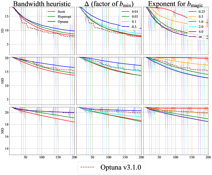
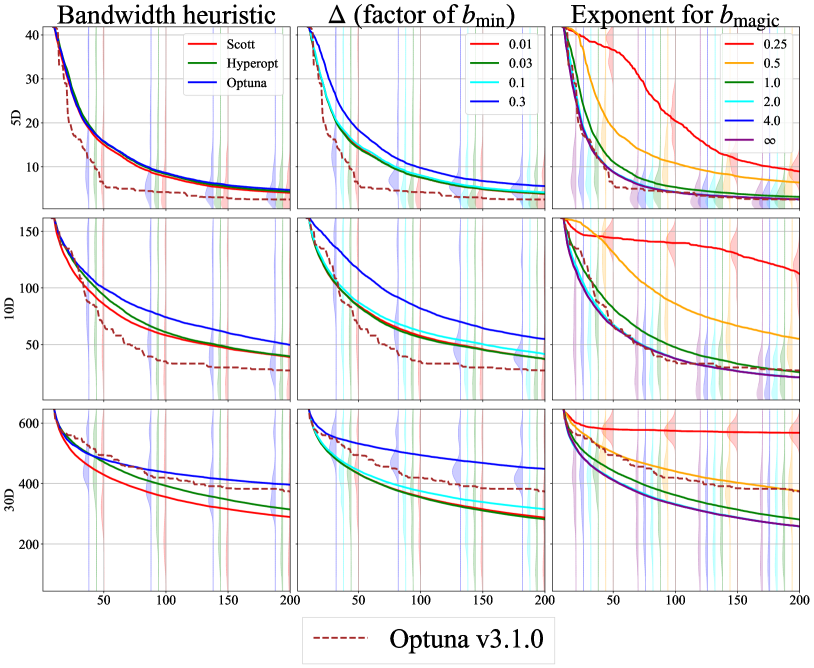
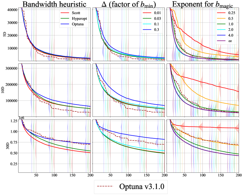
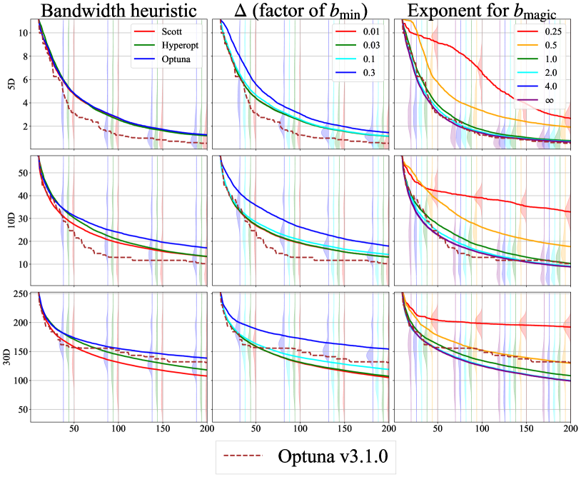
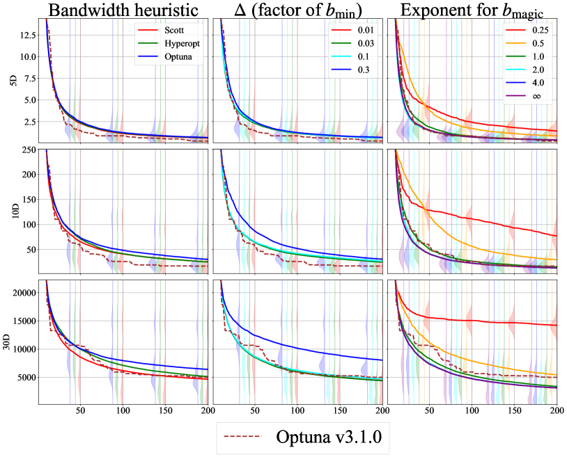
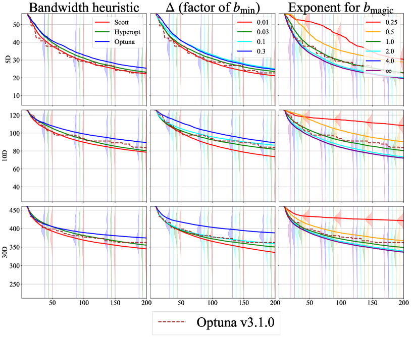
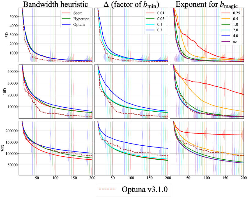
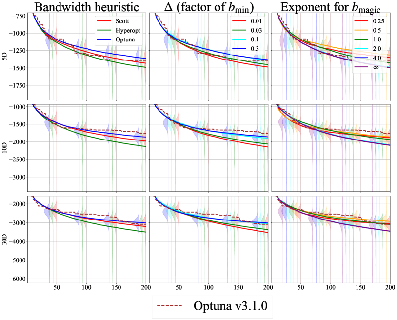
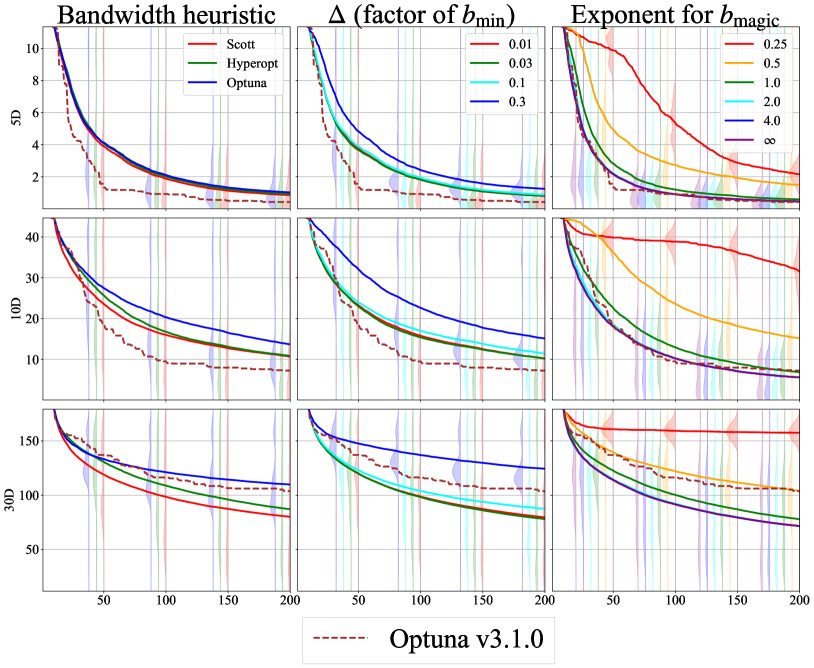
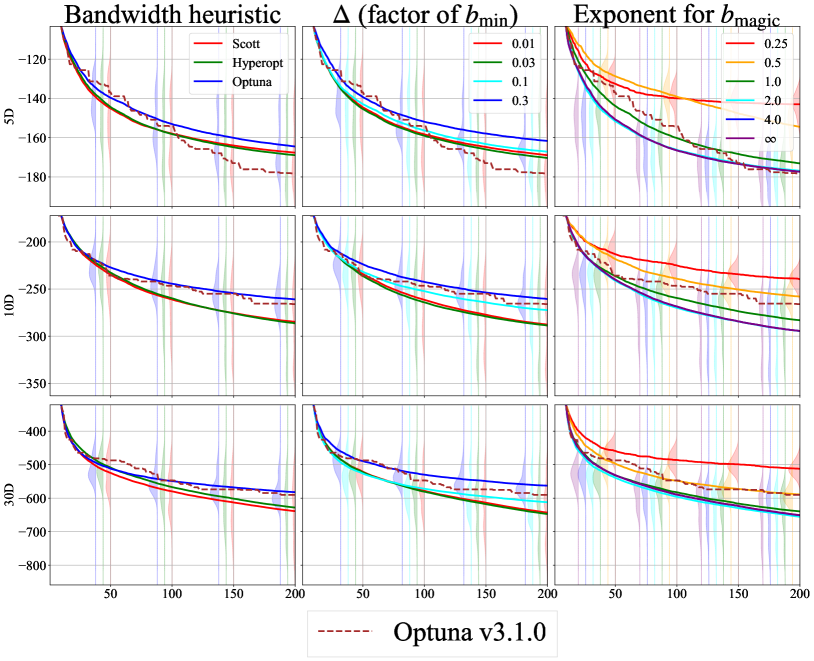
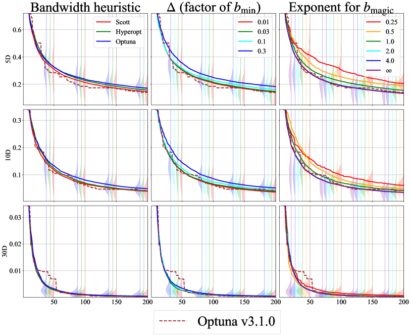
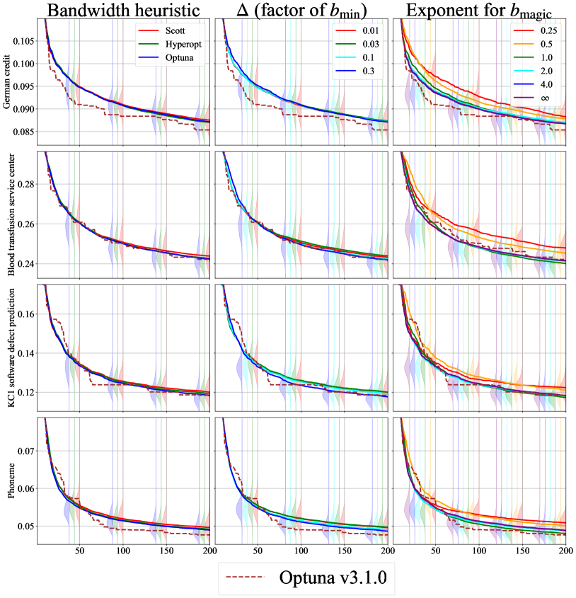
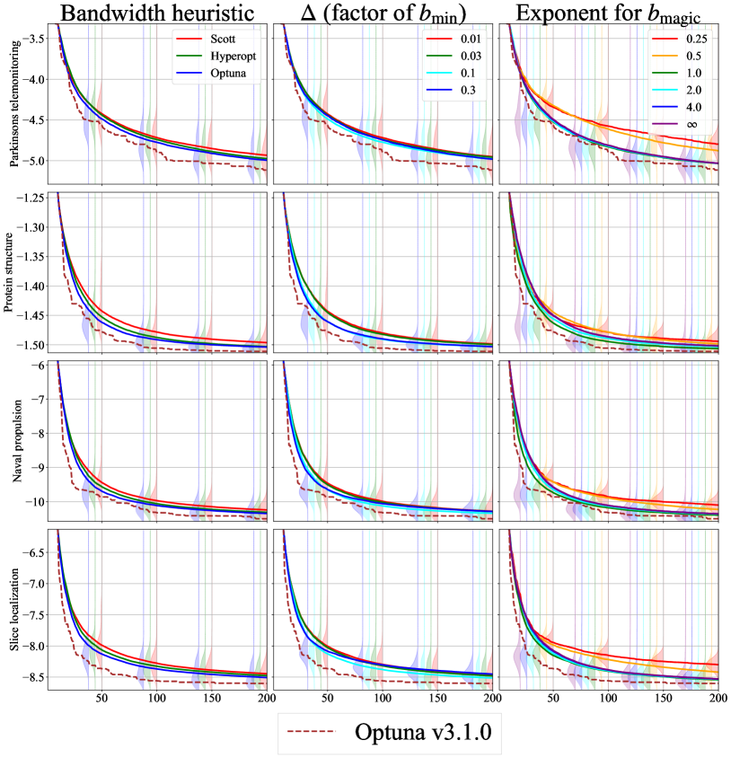
4.2.2 Results & Discussion

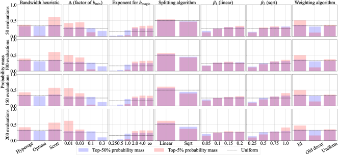
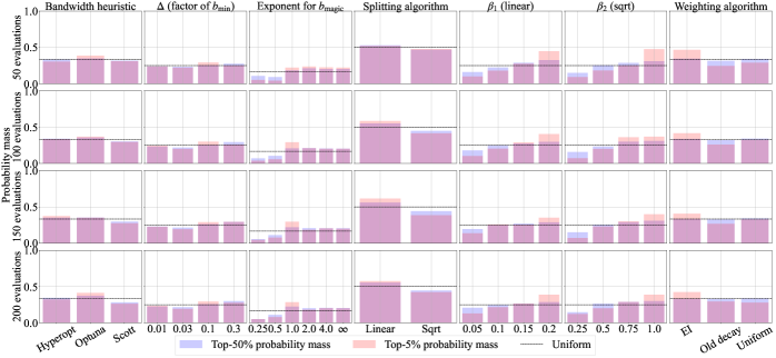
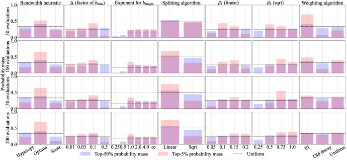
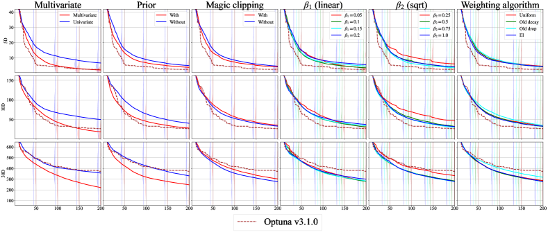
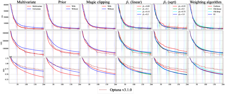
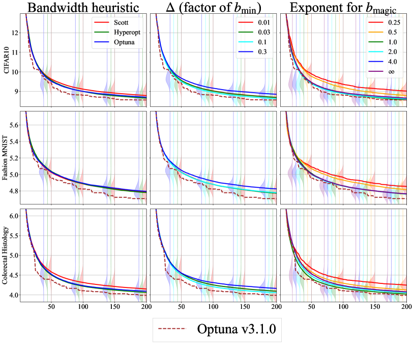
Figures 13,14 present the probability mass of each choice in the top-$50\%$ and -$5\%$ observations and Tables 7,8 present the HPI of each control parameter for the bandwidth selection. Note that since the analysis loses some detailed information, we provided individual results and the details of the analysis in Appendix E.

The minimum bandwidth factor $\Delta$: this factor is the second most important parameter for the benchmark functions and small factors $\Delta=0.01,0.03$ were effective due to the intrinsic cardinality discussed in Section 3.3.4. Although the factor $\Delta$ was not a primarily important parameter for the HPO benchmarks, we might need to take a large $\Delta$ for discrete search spaces, but $\Delta=0.3$ is too large. While we cannot generalize the optimal value $\Delta$ because the noise level of objective functions depends on tasks, our recommendation here is to take $\Delta=0.03$.

The bandwidth selection heuristic: according to the top-$5\%$ probability mass, an appropriate bandwidth selection heuristic varied across tasks. scott was the best choice for the benchmark functions, optuna was the best choice for HPOBench and HPOlib, and hyperopt was the best choice for JAHS-Bench-201. Interestingly, very few settings with optuna could achieve the top-$5\%$ performance on the search spaces with continuous parameters. We found out that this result relates to the minimum bandwidth that each heuristic can take. For example, $b$ takes about $(R-L)/10\sim(R-L)/5$ by optuna based on Eq. (39). However, the result in the minimum bandwidth factor $\Delta$ showed that $\Delta=0.1$ or larger, which makes $b$ be $(R-L)/10$ or larger, exhibits poor performance. It implies that $b$ obtained by optuna is too large for the continuous settings. On the other hand, optuna outperformed the other heuristics on HPOBench and HPOlib. Looking at the peak of the top-$5\%$ probability mass for the factor $\Delta$, we can see that $\Delta=0.1$ has the peak. This explains why optuna, which enforces $b$ to be larger than $(R-L)/10$, outperformed the others in these settings. For scott, we often observed bandwidth for discrete parameters turning zero. Therefore, we need to carefully choose the factor $\Delta$ for the HPO benchmarks when using scott. Although both scott and optuna have clear drawbacks, hyperopt showed the most stable performance due to the natural handling of the intrinsic cardinality, and thus we recommend using hyperopt by default.

The exponent $\alpha$ for $b_{\mathrm{magic}}$: larger $\alpha$, which leads to smaller $b_{\mathrm{magic}}$, was helpful for the benchmark functions, and smaller $\alpha$, which leads to larger $b_{\mathrm{magic}}$, was helpful for the HPO benchmarks as we could expect from Section 4.1.2. As the compromise for both the benchmark functions and the HPO benchmarks lied in $\alpha=2.0$, we recommend using it. However, since the exponent for $b_{\mathrm{magic}}$ is the most important parameter, we need to adapt the parameter carefully.

Splitting and weighting algorithms (gamma, weights): the conclusion for these parameters does not change largely from Section 4.1.2 except we observed that linear with $\beta_{1}=0.15$ generalized the most.

To sum up the results of the ablation study for the bandwidth selection, our recommendation is to use:

1. hyperopt by default, scott for noiseless objectives, and optuna for non-continuous spaces,

2. $\Delta=0.03$ by default, small $\Delta$ ($0.01$ or $0.03$) for noiseless objectives, and large $\Delta$ ($0.03$ or $0.1$) for noisy objectives,

3. $\alpha=2.0$ by default, $\alpha=\infty$ for noiseless objectives, and $\alpha=1.0$ for noisy objectives, and

4. linear with $\beta_{1}=0.15$ (or sqrt with $\beta_{2}=0.75$) and weights=EI.

In the next section, we validate the performance of our recommended setting against recent BO methods.

4.3 Comparison with Baseline Methods

In this experiment, we compare TPE with the recommended setting to various BO methods to show the improvement we made.

4.3.1 Setup

In this section, we compare our TPE with the following baseline methods:

• BORE (?): a classifier-based BO method inspired by TPE,

• HEBO  (?): the winner solution of the black-box optimization challenge 2020 (?),

• Random search (?): the most basic baseline method in HPO,

• SMAC  (?, ?): a random forest-based BO method widely used in practice, and

• TurBO  (?): a recent strong baseline method used in the black-box optimization challenge 2020.

We used the default settings in each package and we followed the default setting of Syne Tune (?) for BORE, which did not specify its default classifier in the original paper (?). More specifically, we used XGBoost as a classifier model in BORE and picked the best candidate point among $500$ random candidate points. For TurBO, we used the default setting in SMAC3 and it uses TurBO-1 where TurBO-M refers to TurBO with $M$ trust regions. Since HPOlib and JAHS-Bench-201 include categorical parameters, we applied one-hot encoding to the categorical parameters in each benchmark for the Gaussian process-based BOs, which are TurBO and HEBO.

For TPE, we fixed each control parameter as follows:

• multivariate=True,

• consider_prior=True,

• consider_magic_clip=True with the exponent $\alpha=2.0$ for $b_{\mathrm{magic}}$,

• gamma=linear with $\beta=0.15$,

• weights=EI,

• optuna for the categorical bandwidth selection,

• hyperopt for the bandwidth selection heuristic, and

• the minimum bandwidth factor $\Delta=0.03$.

Furthermore, we run Optuna v3.1.0 and Hyperopt v0.2.7, both of which use TPE internally, to see the improvements. For the visualization, we used the average rank of the median performance over $10$ random seeds.

Figure 15: The average rank of each optimization method. Since all the optimization methods shared initial configurations, the initial average ranks are constant. Note that since we could not run SMAC3 on JAHS-Bench-201 due to a package dependency issue, we omitted SMAC for JAHS-Bench-201. We provide the individual results in Appendix E.3.

Figure 16: The cumulative runtime of each optimization method on the sphere function with different dimensionalities (5D for Left, 10D for Center, and 30D for Right). The horizontal axis is the number of configuration evaluations and the weak-color bands show the standard error over $10$ independent runs. Note that we used 8 cores of Intel Core i7-10700.

Table 9: The qualitative summary of the results obtained from the comparison. As only HEBO, TurBO, and our TPE exhibited the strongest performance, we describe only three of them. We qualitatively rated each column for each method by $\bigcirc$ (relatively good), $\triangle$ (medium), and $\times$ (relatively bad).

	Runtime	Continuous (Low/High dimensional)		Discrete (W/O categorical)
		Low ($\sim 15\mathrm{D}$)	High ($15\mathrm{D}\sim$)	With	Without
Our TPE	$\bigcirc$	$\triangle$	$\triangle$	$\bigcirc$	$\triangle$
HEBO	$\times$	$\bigcirc$	$\times$	$\bigcirc$	$\bigcirc$
TurBO	$\triangle$	$\triangle$	$\bigcirc$	$\times$	$\triangle$

(a) A setting adapted to the benchmark functions

(b) A setting adapted to the tabular benchmarks

Figure 17: The settings adapted for each problem setting. To adapt to the benchmark functions (Top), we used gamma=linear with $\beta=0.1$, weights=EI, consider_magic_clip=False, the heuristic of scott, and $\Delta=0.01$. To adapt to the tabular benchmarks (Bottom), we used gamma=linear with $\beta=0.15$, weights=EI, consider_magic_clip=True with $\alpha=1.0$, the heuristic of optuna, and $\Delta=0.1$.

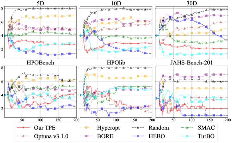
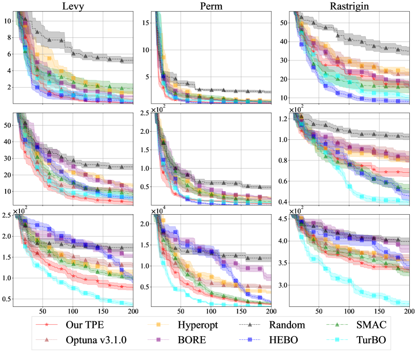
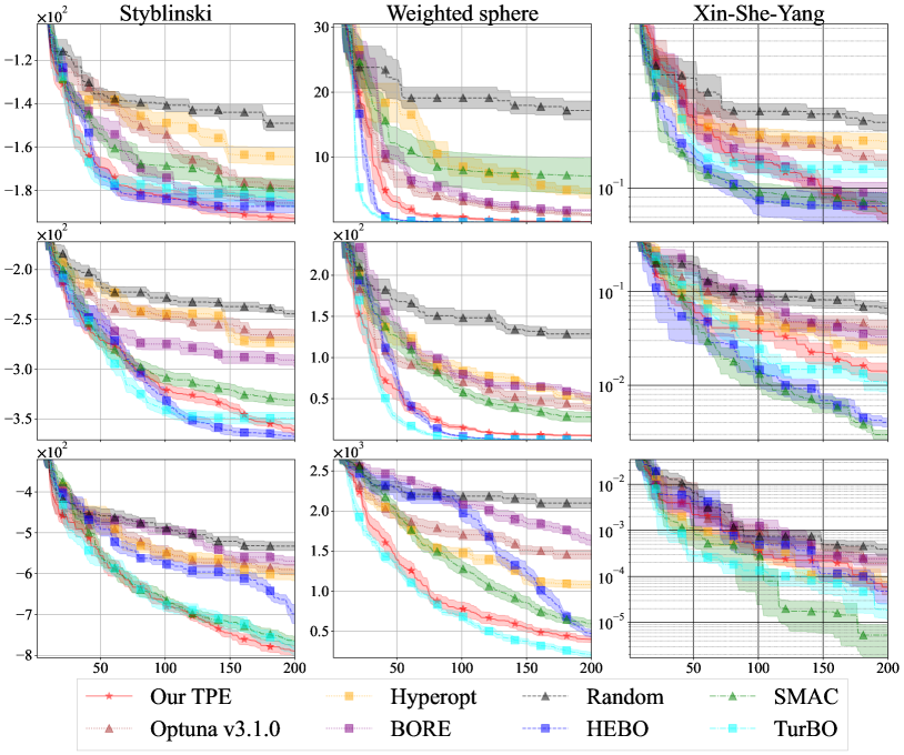
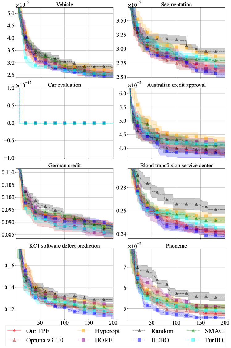
4.3.2 Results & Discussion

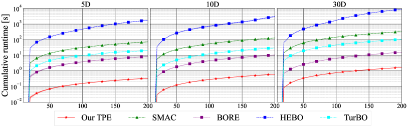
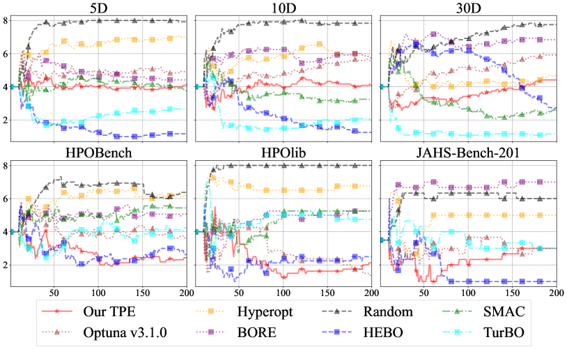
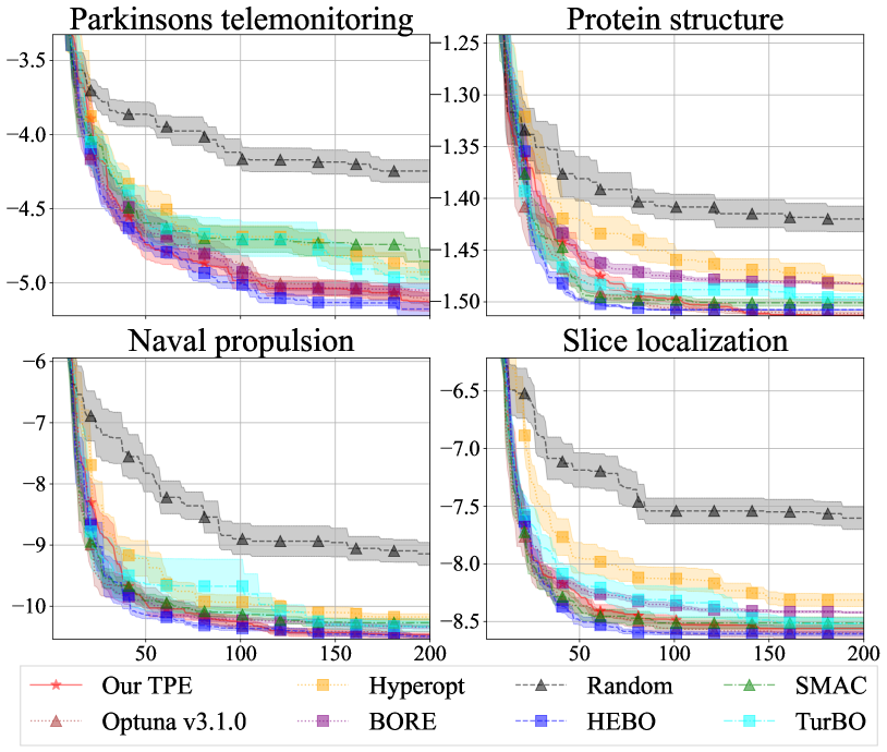
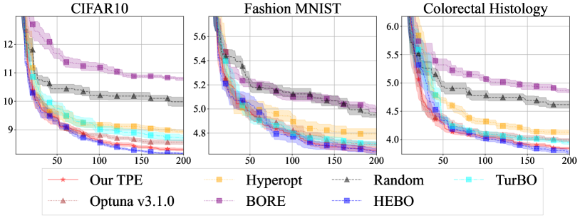
Figure 15 presents the average rank of each optimization method and we provided the individual results in Appendix E.3. We first would like to mention that Hyperopt is used for the TPE algorithm in most research papers. However, we found out that the Hyperopt implementation exhibited much worse performance and our recommended setting achieved much better generalization. For the benchmark functions, TurBO and HEBO exhibited strong performance compared to our TPE. While the performance of TurBO was degraded for the HPO benchmarks, HEBO consistently achieved the top performance on the HPO benchmarks. Although our TPE could not outperform HEBO except for the 30D problems, our TPE is much quicker compared to HEBO, which takes $2.5$ hours to sample $200$ configurations on the 30D problems, as shown in Figure 16. Since the computational burden of an objective varies, we need to carefully choose an optimization method. For example, if the evaluation of an objective takes only a few seconds, HEBO is probably not an appropriate choice as the sampling at each iteration dominates the evaluation of the objective. We summarized the qualitative evaluations in Table 9.

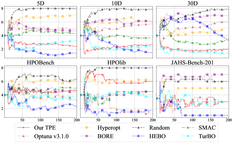
Finally, we show the comparisons using the adapted setting concluded in Section 4.2.2. Figure 17 presents the average ranks of our TPE using the settings for the benchmark functions and the tabular benchmarks. The results indicate that our TPE with the adapted settings can be competitive to the top performance in exchange for the performance degradation on the problems that are out of scope. Although these results do not guarantee that the adapted settings will be effective for an arbitrary set of benchmark functions or tabular benchmarks, we can expect stronger performance on many problem settings.

5 Conclusion

In this paper, we provided detailed explanations of each component in the TPE algorithm and showed how we should determine each control parameter. Roughly speaking, the control parameter settings should be changed depending on how much noise objective functions have and the bandwidth selection algorithm is especially important to be carefully tuned due to the variation of the intrinsic cardinality. Despite that, we also provided the default recommended setting as a conclusion and we compared our recommended version of TPE with various baseline methods in the last experiment. The results demonstrated that our TPE could perform much better than the existing TPE-related packages such as Hyperopt and Optuna and potentially outperform the state-of-the-art BO methods with much fewer computational requirements. As we focused on the single-objective optimization setting, we did not discuss settings such as multi-objective, constrained, multi-fidelity, and batch optimization and the investigation of these settings would be our future works.

A The Derivation of the Acquisition Function

Under the assumption in Eq. (6), EI and PI are equivalent (?, ?, ?). For this reason, we only discuss PI for simplicity. We show the detail of the transformations to obtain Eq. (8). We first plug in Eq. (6) to Eq. (3) (the formulation of PI) as follows:

$$\int_{-\infty}^{y^{\gamma}}p(y|\bm{x},\mathcal{D})dy =\int_{-\infty}^{y^{\gamma}}\frac{p(\bm{x}|y,\mathcal{D})p(y|\mathcal{D})}{p(\bm{x}|\mathcal{D})}dy~{}(\because\mathrm{Bayes^{\prime}~{}theorem})$$ (31)

$$=\frac{p(\bm{x}|\mathcal{D}^{(l)})}{p(\bm{x}|\mathcal{D})}\underbrace{\int_{-\infty}^{y^{\gamma}}p(y|\mathcal{D})dy}_{=\gamma}~{}(\because y\in(-\infty,y^{\gamma}]\Rightarrow p(\bm{x}|y,\mathcal{D})=p(\bm{x}|\mathcal{D}^{(l)}))$$

$$=\frac{\gamma p(\bm{x}|\mathcal{D}^{(l)})}{\gamma p(\bm{x}|\mathcal{D}^{(l)})+(1-\gamma)p(\bm{x}|\mathcal{D}^{(g)})}$$

where the last transformation used the following marginalization:

$$p(\bm{x}|\mathcal{D}) =\int_{-\infty}^{\infty}p(\bm{x}|y,\mathcal{D})p(y|\mathcal{D})dy$$ (32)

$$=p(\bm{x}|\mathcal{D}^{(l)})\int_{-\infty}^{y^{\gamma}}p(y|\mathcal{D})dy+p(\bm{x}|\mathcal{D}^{(g)})\int_{y^{\gamma}}^{\infty}p(y|\mathcal{D})dy$$

$$=\gamma p(\bm{x}|\mathcal{D}^{(l)})+(1-\gamma)p(\bm{x}|\mathcal{D}^{(g)}).$$

B Related Work of Tree-Structured Parzen Estimator

In this paper, while we discussed only the single-objective setting, there are strict generalizations with multi-objective (MO-TPE) (?, ?) and constrained optimization (c-TPE) (?) settings. More specifically, the algorithm of MOTPE is identical to the original TPE when the number of objectives is 1 and that of c-TPE is identical to the original TPE when the violation probability is almost everywhere zero, i.e. $\mathbb{P}[\bigcap_{i=1}^{K}c_{i}\leq c_{i}^{\star}|\bm{x}]=0$ for almost all  $\bm{x}\in\mathcal{X}$. TPE also has extensions for the multi-fidelity and meta-learning settings. ? (?) extended TPE to the multi-fidelity setting by combining TPE and Hyperband (?). ? (?) introduced meta-learning by considering task similarity via the overlap of promising domains.

Furthermore, ? (?) introduced BORE inspired by TPE. BORE replaces the density ratio with a classifier model based on the fact that TPE evaluates the promise of configurations by binary classification. ? (?) and ? (?) built some theories on top of BORE. ? (?) formally derived the expected improvement when we use a classifier model instead of a regression model. While TPE and BORE train a binary classifier with uniform weights for each sample, the expected improvement requires a binary classifier with different weights depending on the improvement from a given threshold. ? (?) provided a theoretical analysis of regret using the Gaussian process classifier. In contrast to BORE, TPE has almost no theories due to the multimodality nature of KDE and the explicit handling of density ratio. To the best of our knowledge, the only theory is about the convergence of the better group $\mathcal{D}^{(l)}$. ? (?) showed that $\mathcal{D}^{(l)}$ asymptotically converges to a set of the $\gamma^{\prime}$-quantile ($\gamma^{\prime}<\gamma$) configurations if the objective function $f$ does not have noise, we use the $\epsilon$-greedy algorithm in Line 14, and we use a fixed $\gamma$. This result suggests that we should pick a random configuration once in a while although we did not use the $\epsilon$-greedy algorithm because of our severely limited computational settings. In this paper, however, we only focus on TPE, but not methods using another classifier such as BORE (?) and LFBO (?).

C More Details of Kernel Density Estimator

In this section, we describe the implementation details of kernel density estimator used in each package.

C.1 Uniform Weighting Algorithm in BOHB

Suppose we have $\{x_{n}\}_{n=1}^{N}$ and we would like to build a KDE for $x\in[L,R]$, then the KDE is defined in BOHB as follows:

$$\sum_{n=1}^{N}\frac{z_{n}}{\sum_{i=1}^{N}z_{i}}g(x,x_{n}|b)$$ (33)

where $g$ is defined in Eq. (22) and $z_{n}=\int_{L}^{R}g(x,x_{n})dx$. In principle, this formulation allows to flatten PDFs even when the observations concentrate near a boundary. Note that we did not use this formulation in the experiments although we also regard this formulation as uniform.

C.2 group Parameter in Optuna for the Multivariate Kernel

In this section, we use the symbol $x_{\mathrm{null}}$ to refer to an undefined value and we use $\mathbb{R}_{\mathrm{null}}\coloneqq\mathbb{R}\cup\{x_{\mathrm{null}}\}$ for convenience.

We first formally define the tree-structured search space. Suppose $\mathcal{X}\coloneqq\mathcal{X}_{1}\times\mathcal{X}_{2}\times\dots\mathcal{X}_{D}$ is a $D$-dimensional search space with $\mathcal{X}_{d}\subseteq\mathbb{R}_{\mathrm{null}}$ for each $d\in[D]\coloneqq\{1,\dots,D\}$ and the $d_{i}$-th ($d_{i}\in[D]$) dimension is conditional for each $i\in[D_{c}]$ where $D_{c}(<D)$ is the number of conditional parameters. Furthermore, we assume that practitioners provide binary functions $c_{d_{i}}:\prod_{d\neq d_{i}}\mathcal{X}_{d}\rightarrow\{0,1\}$ for each $i\in[D_{c}]$. For example, when we optimize the following parameters of a neural network:

• The number of layers $x_{1}\coloneqq L\in[3]=\mathcal{X}_{1}$, and

• The dropout rates at the $l$-th layer $x_{l+1}\coloneqq p_{l}\in[0,1]=\mathcal{X}_{l+1}$ for $l\in[3]$,

then $x_{3}$ and $x_{4}$ are the conditional parameters in this search space. The binary functions for this search space are $c_{3}(x_{1},x_{2},x_{4})=\mathbb{I}[x_{1}\geq 2]=\mathbb{I}[L\geq 2]$ and $c_{4}(x_{1},x_{2},x_{3})=\mathbb{I}[x_{1}\geq 3]=\mathbb{I}[L\geq 3]$. Note that the dropout rate at the $l$-th layer will not be defined if there are no more than $l$ layers. Another example is the following search space of a neural network:

• The number of layers $x_{1}\coloneqq L\in[2]=\mathcal{X}_{1}$,

• The optimizer at the $1$st layer $x_{2}\in\{\mathtt{adam},\mathtt{sgd}\}=\mathcal{X}_{2}$ ,

• The coefficient $\beta_{1}\in(0,1)=\mathcal{X}_{3}$ for adam in the 1st layer,

• The coefficient $\beta_{2}\in(0,1)=\mathcal{X}_{4}$ for adam in the 1st layer,

• The momentum $m\in(0,1)=\mathcal{X}_{5}$ for sgd in the 1st layer,

• The optimizer at the $2$nd layer $x_{6}\in\{\mathtt{adam},\mathtt{sgd}\}=\mathcal{X}_{6}$,

• The coefficient $\beta_{1}\in(0,1)=\mathcal{X}_{7}$ for adam in the 2nd layer,

• The coefficient $\beta_{2}\in(0,1)=\mathcal{X}_{8}$ for adam in the 2nd layer, and

• The momentum $m\in(0,1)=\mathcal{X}_{9}$ for sgd in the 2nd layer.

In this example, all the parameters except $x_{1},x_{2}$ are conditional. The binary functions for each dimension are computed as follows:

• $c_{3}=c_{4}=\mathbb{I}[x_{2}=\mathtt{adam}]$,

• $c_{5}=\mathbb{I}[x_{2}=\mathtt{sgd}]$,

• $c_{6}=\mathbb{I}[x_{1}\geq 2]$,

• $c_{7}=c_{8}=\mathbb{I}[x_{1}\geq 2]\mathbb{I}[x_{6}=\mathtt{adam}]$, and

• $c_{9}=\mathbb{I}[x_{1}\geq 2]\mathbb{I}[x_{6}=\mathtt{sgd}]$.

As can be seen, $x_{7},x_{8},x_{9}$ require $x_{6}$ to be defined and $x_{6}$ requires $x_{1}$ to be no less than $2$. This hierarchical structure, i.e. $x_{7},x_{8},x_{9}$ require $x_{6}$ and, in turn, $x_{1}$ as well to be defined, is the exact reason why we call search spaces with conditional parameters tree-structured. Strictly speaking, we cannot provide $x_{7},x_{8},x_{9}$ to $c_{6}$, but we do not need them for $c_{6}$ due to the tree structure, and thus we provide $x_{\mathrm{null}}$ for $x_{7},x_{8},x_{9}$ instead.

Using the second example above, we will explain the group parameter in Optuna. First, we define a set of dimensions as $s\subseteq[D]$ and a subspace of $\mathcal{X}$ that takes the dimensions specified in $s$ as $\mathcal{X}_{s}\coloneqq\prod_{d\in s}\mathcal{X}_{d}$. Then group enumerates all possible $\mathcal{X}_{s}$ based on a set of observations $\mathcal{D}$ and optimizes the acquisition function separately in each subspace. For example, the second example above could take $\mathcal{X}_{\{1,2,3,4\}}$, $\mathcal{X}_{\{1,2,5\}}$, $\mathcal{X}_{\{1,2,3,4,6,7,8\}}$, $\mathcal{X}_{\{1,2,3,4,6,9\}}$, $\mathcal{X}_{\{1,2,5,6,7,8\}}$, and $\mathcal{X}_{\{1,2,5,6,9\}}$, as subspaces when we ignore dimensions that have $x_{\mathrm{null}}$. The enumeration of the subspaces could be easily reproduced by checking missing values in each observation from $\mathcal{D}$ with the time complexity of $O(DN)$. Then we perform a sampling by the TPE algorithm in each subspace using the observations that belong exactly to $\mathcal{X}_{s}$ when we ignore $x_{\mathrm{null}}$. In other words, when we have an observation $\{2,\mathtt{sgd},x_{\mathrm{null}},x_{\mathrm{null}},0.5,\mathtt{sgd},x_{\mathrm{null}},x_{\mathrm{null}},0.5\}$, we use this observation only for the sampling in $\mathcal{X}_{\{1,2,5,6,9\}}$, but not for that in $\mathcal{X}_{\{1,2,5\}}$.

C.3 Bandwidth Selection

Throughout this section, we assume that we compute the bandwidth of KDE based on a set of observations $\{x_{n}\}_{n=1}^{N}\in[L,R]^{N}$ where $x_{n}$ is sorted so that it satisfies $x_{1}\leq x_{2}\leq\dots\leq x_{N}$ and the observations also include the prior $x=(L+R)/2$ if we include the prior. Note that all methods select the bandwidth for each dimension independently of each other.

C.3.1 Hyperopt Implementation

When consider_endpoints=True, we first augment the observations as $\{x_{n}\}_{n=0}^{N+1}$ where $x_{0}=L,x_{N+1}=R$; otherwise, we just use $\{x_{n}\}_{n=1}^{N}$. Then the bandwidth $b_{n}$ for the $n$-th kernel function $k(\cdot,x_{n}|b_{n})$ ($n=1,2,\dots,N$) is computed as follows:

$$b_{n}\coloneqq\left\{\begin{array}[]{ll}x_{n}-x_{n-1}&(\mathrm{if}~{}x_{n+1}~{}\mathrm{not~{}exist})\\ x_{n+1}-x_{n}&(\mathrm{if}~{}x_{n-1}~{}\mathrm{not~{}exist})\\ \max(\{x_{n+1}-x_{n},x_{n}-x_{n-1}\})&(\mathrm{otherwise})\\ \end{array}\right..$$ (37)

This heuristic allows us to adapt the bandwidth depending on the concentration of observations. More specifically, the bandwidth will be wider if a region has few observations while the bandwidth will be narrower if a region has many observations.

C.3.2 BOHB Implementation (Scott’s Rule)

For the univariate Gaussian kernel, Scott’s rule calculates bandwidth as follows:

$$b=\biggl{(}\frac{4}{3N}\biggr{)}^{1/5}\min\biggl{(}\sigma,\frac{\mathrm{IQR}}{\Phi^{-1}(0.75)-\Phi^{-1}(0.25)}\biggr{)}\simeq 1.059N^{-1/5}\min\biggl{(}\sigma,\frac{\mathrm{IQR}}{1.34}\biggr{)}$$ (38)

where $(4/3N)^{1/5}$ comes from Eq. (3.28) by ? (?), $\mathrm{IQR}$ is the interquartile range of the observations, $\sigma$ is the standard deviation of the observations, and $\Phi:\mathbb{R}\rightarrow[0,1]$ is the cumulative distribution of $\mathcal{N}(0,1)$. BOHB calculates the bandwidth for each dimension separately and calculates the bandwidth for categorical parameters as if they are numerical parameters.

C.3.3 Optuna v3.1.0 Implementation

In contrast, the bandwidth is computed in Optuna v3.1.0 as follows:

$$b=\frac{R-L}{5}N^{-1/(D+4)}$$ (39)

where $D$ is the dimension of search space, $N$ is the number of observations, and the domain of the target parameter is $[L,R]$. Note that it is obvious from the formulation, but the constant factor $N^{-1/(D+4)}/5$ of the bandwidth is fixed for all dimensions.

For the Aitchison-Aitken kernel, the categorical bandwidth is determined in Optuna v3.1.0 as follows:

$$b=\frac{1+1/N}{1+C/N}$$ (40)

where $N$ is the number of observations, and $C\in\mathbb{Z}_{+}$ is the number of categories.

Table 10: The list of the benchmark functions. Each function can take an arbitrary dimension $D\in\mathbb{Z}_{+}$. The right column shows the domain of each function. In the experiments, we used one of the dimensions $D\in\{5,10,30\}$.

Name $f(\bm{x})$ ($\bm{x}\coloneqq[x_{1},x_{2},\dots,x_{D}]$) $|x_{d}|\leq R$ Ackley $\exp(1)+20\biggl{(}1-\exp\biggl{(}-\frac{1}{5}\sqrt{\frac{1}{D}\sum_{d=1}^{D}x_{d}^{2}}\biggr{)}\biggr{)}-\exp\biggl{(}\frac{1}{D}\sum_{d=1}^{D}\cos 2\pi x_{d}\biggr{)}$ $32.768$ Griewank $1+\frac{1}{4000}\sum_{d=1}^{D}x_{d}^{2}-\prod_{d=1}^{D}\cos\frac{x_{d}}{\sqrt{d}}$ $600$ K-Tablet $\sum_{d=1}^{K}x_{d}^{2}+\sum_{d=K+1}^{D}(100x_{d})^{2}$ where $K=\lceil D/4\rceil$ $5.12$ Levy $\sin^{2}\pi w_{1}+\sum_{d=1}^{D-1}(w_{d}-1)^{2}(1+10\sin^{2}(\pi w_{d}+1))+(w_{D}-1)^{2}(1+\sin^{2}2\pi w_{D})$ $10$ where $w_{d}=1+\frac{x_{d}-1}{4}$ Perm $\sum_{d_{1}=1}^{D}\biggl{(}\sum_{d_{2}=1}^{D}(d_{2}+1)(x_{d_{2}}^{d_{1}}-\frac{1}{{d_{2}}^{d_{1}}})\biggr{)}^{2}$ $1$ Rastrigin $10D+\sum_{d=1}^{D}(x_{d}^{2}-10\cos 2\pi x_{d})$ $5.12$ Rosenbrock $\sum_{d=1}^{D-1}\biggl{(}100(x_{d+1}-x_{d}^{2})^{2}+(x_{d}-1)^{2}\biggr{)}$ $5$ Schwefel $-\sum_{d=1}^{D}x_{d}\sin\sqrt{|x_{d}|}$ $500$ Sphere $\sum_{d=1}^{D}x_{d}^{2}$ $5$ Styblinski $\frac{1}{2}\sum_{d=1}^{D}(x_{d}^{4}-16x_{d}^{2}+5x_{d})$ $5$ Weighted sphere $\sum_{d=1}^{D}dx_{d}^{2}$ $5$ Xin-She-Yang $\sum_{d_{1}=1}^{D}|x_{d_{1}}|\exp\biggl{(}-\sum_{d_{2}=1}^{D}\sin x_{d_{2}}^{2}\biggr{)}$ $2\pi$

Table 11: The characteristics of the benchmark functions.

Name Characteristics Ackley Multimodal Griewank Multimodal K-Tablet Monomodal, ill-conditioned Levy Multimodal Perm Monomodal Rastrigin Multimodal Rosenbrock Monomodal Schwefel Multimodal Sphere Convex, monomodal Styblinski Multimodal Weighted sphere Convex, monomodal Xin-She-Yang Multimodal

Table 12: The search space of HPOBench (5 discrete parameters). HPOBench is a tabular benchmark and we can query the performance of a specified configuration from the tabular. HPOBench stores all possible configurations of an MLP in this table for 8 different OpenML datasets (Vehicle, Segmentation, Car evaluation, Australian credit approval, German credit, Blood transfusion service center, KC1 software detect prediction, Phoneme). Each parameter except “Depth” has 10 grids and the grids are taken so that each grid is equally distributed in the log-scaled range.

Hyperparameter	Parameter type	Range
L2 regularization	Discrete	$[10^{-8},1]$
Batch size	Discrete	$[4,256]$
Depth	Discrete	$[1,3]$
Initial learning rate	Discrete	$[10^{-5},1]$
Width	Discrete	$[16,1024]$

Table 13: The search space of HPOlib (6 discrete + 3 categorical parameters). HPOlib is a tabular benchmark and we can query the performance of a specified configuration from the tabular. HPOlib stores all possible configurations of an MLP in this table for 4 different datasets (Parkinsons telemonitoring, Protein structure, Naval propulsion, Slice localization).

Hyperparameter Parameter type Range Initial learning rate Discrete $\{5\times 10^{-4},10^{-3},5\times 10^{-3},10^{-2},5\times 10^{-2},10^{-1}\}$ Dropout rate {1, 2} Discrete $\{0.0,0.3,0.6\}$ Number of units {1, 2} Discrete $\{2^{4},2^{5},2^{6},2^{7},2^{8},2^{9}\}$ Batch size Discrete $\{2^{3},2^{4},2^{5},2^{6}\}$ Learning rate scheduling Categorical {cosine, constant} Activation function {1, 2} Categorical {ReLU, tanh}

Table 14: The search space of JAHS-Bench-201 (2 continuous + 2 discrete + 8 categorical parameters). JAHS-Bench-201 is a surrogate benchmark and it uses an XGBoost surrogate model trained on pre-evaluated configurations for 3 different datasets (CIFAR10, Fashion MNIST, Colorectal histology). We use the output of the XGBoost surrogate given a specified configuration as a query.

Hyperparameter Parameter type Range Learning rate Continuous $[10^{-3},1]$ L2 regularization Continuous $[10^{-5},10^{-2}]$ Depth multiplier Discrete $\{1,2,3\}$ Width multiplier Discrete $\{2^{2},2^{3},2^{4}\}$ Cell search space Categorical {none, avg-pool-3x3, bn-conv-1x1, (NAS-Bench-201 (?), Edge 1 – 6) bn-conv-3x3, skip-connection} Activation function Categorical {ReLU, Hardswish, Mish} Trivial augment (?) Categorical {True, False}

D The Details of Benchmarks

For the benchmark functions, we used $12$ different functions in Table 10 with $3$ different dimensionalities. The characteristics of each benchmark function are available in Table 11 For the HPO benchmarks, we used HPOBench (?) in Table 12, HPOlib (?) in Table 13, and JAHS-Bench-201 (?) in Table 14. In HPO benchmarks, there are two types:

1. tabular benchmark, which queries pre-recorded performance metric values from a static table which is why it cannot handle continuous parameters, and

2. surrogate benchmark, which returns the predicted performance metric values by a surrogate model for the corresponding HP configurations.

HPOlib and HPOBench are tabular benchmarks and JAHS-Bench-201 is a surrogate benchmark.

(a) Ackley with 5D (Top row), 10D (Middle row), and 30D (Bottom row)

(b) Griewank with 5D (Top row), 10D (Middle row), and 30D (Bottom row)

(c) K-Tablet with 5D (Top row), 10D (Middle row), and 30D (Bottom row)

Figure 18: The ablation study on benchmark functions. The $x$-axis is the number of evaluations and the $y$-axis is the cumulative minimum objective. The solid lines in each figure shows the mean of the cumulative minimum objective over all control parameter configurations. The transparent shades represent the distributions of the cumulative minimum objective at $\{50,100,150,200\}$ evaluations. For baselines, we provide the performance of Optuna v3.1.0 (brown dotted lines).

(a) Levy with 5D (Top row), 10D (Middle row), and 30D (Bottom row)

(b) Perm with 5D (Top row), 10D (Middle row), and 30D (Bottom row)

(c) Rastrigin with 5D (Top row), 10D (Middle row), and 30D (Bottom row)

Figure 19: The ablation study on benchmark functions. The $x$-axis is the number of evaluations and the $y$-axis is the cumulative minimum objective. The solid lines in each figure shows the mean of the cumulative minimum objective over all control parameter configurations. The transparent shades represent the distributions of the cumulative minimum objective at $\{50,100,150,200\}$ evaluations. For baselines, we provide the performance of Optuna v3.1.0 (brown dotted lines).

(a) Rosenbrock with 5D (Top row), 10D (Middle row), and 30D (Bottom row)

(b) Schwefel with 5D (Top row), 10D (Middle row), and 30D (Bottom row)

(c) Sphere with 5D (Top row), 10D (Middle row), and 30D (Bottom row)

Figure 20: The ablation study on benchmark functions. The $x$-axis is the number of evaluations and the $y$-axis is the cumulative minimum objective. The solid lines in each figure shows the mean of the cumulative minimum objective over all control parameter configurations. The transparent shades represent the distributions of the cumulative minimum objective at $\{50,100,150,200\}$ evaluations. For baselines, we provide the performance of Optuna v3.1.0 (brown dotted lines).

(a) Styblinski with 5D (Top row), 10D (Middle row), and 30D (Bottom row)

(b) Weighted sphere with 5D (Top row), 10D (Middle row), and 30D (Bottom row)

(c) Xin-She-Yang with 5D (Top row), 10D (Middle row), and 30D (Bottom row)

Figure 21: The ablation study on benchmark functions. The $x$-axis is the number of evaluations and the $y$-axis is the cumulative minimum objective. The solid lines in each figure shows the mean of the cumulative minimum objective over all control parameter configurations. The transparent shades represent the distributions of the cumulative minimum objective at $\{50,100,150,200\}$ evaluations. For baselines, we provide the performance of Optuna v3.1.0 (brown dotted lines).

Figure 22: The ablation study on HPOBench ($8$ tasks). The $x$-axis is the number of evaluations and the $y$-axis is the cumulative minimum objective. The solid lines in each figure shows the mean of the cumulative minimum objective over all control parameter configurations. The transparent shades represent the distributions of the cumulative minimum objective at $\{50,100,150,200\}$ evaluations. For baselines, we provide the performance of Optuna v3.1.0 (brown dotted lines).

(a) HPOlib

(b) JAHS-Bench-201

Figure 23: The ablation study on HPOlib ($4$ tasks) and JAHS-Bench-201 ($3$ tasks), which have categorical parameters. The $x$-axis is the number of evaluations and the $y$-axis is the cumulative minimum objective. The solid lines in each figure shows the mean of the cumulative minimum objective over all control parameter configurations. Note that the objective of HPOlib is the $\log$ of validation mean squared error. The transparent shades represent the distributions of the cumulative minimum objective at $\{50,100,150,200\}$ evaluations. For baselines, we provide the performance of Optuna v3.1.0 (brown dotted lines).

E Additional Results

In this section, we provide additional results. For the visualization of figures, we performed the following operations (see the notations invented in Section 4.1.1):

1. Fix a control parameter (e.g. multivariate=True),

2. Gather all the cumulative minimum performance curves $\{\{\zeta_{k,n}^{(m)}\}_{k=1}^{K}\}_{n=1}^{N}$ where $N=200$ was used in the experiments,

3. Plot the mean value $1/K\sum_{k=1}^{K}\zeta_{k,n}^{(m)}$ over the gathered results at each “$n$ evaluations” ($n=1,\dots,N$) as a solid line,

4. Plot vertically the (violin-plot-like) distribution of the gathered results $\{\zeta_{k,n}^{(m)}\}_{k=1}^{K}$ at $n\in\{50,100,150,200\}$ evaluations as a transparent shadow, and

5. Repeat Operations 1.–4. for all settings.

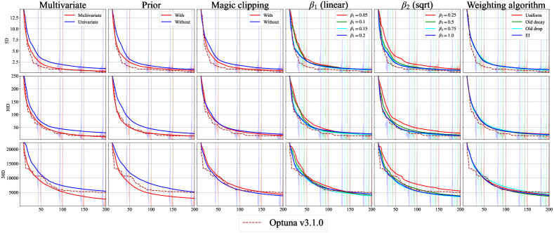
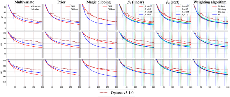
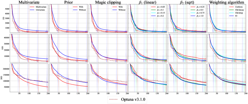
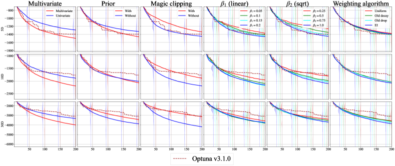
Since the standard error loses the distributional information, we used the violin-plot-like distributions instead. Furthermore, each result includes optimizations by Optuna v3.1.0 as a baseline.

E.1 Ablation Study

Figures 18–21 present the results on the benchmark functions and Figures 22,23 present the results on the HPO benchmarks.

E.2 Analysis of the Bandwidth Selection

Figures 24–35 present the results on the benchmark functions and Figures 36–39 present the results on the HPO benchmarks.

Figure 24: The ablation study of bandwidth related algorithms on the Ackley function. The $x$-axis is the number of evaluations and the $y$-axis is the cumulative minimum objective. The solid lines in each figure shows the mean of the cumulative minimum objective over all control parameter configurations. The transparent shades represent the distributions of the cumulative minimum objective at $\{50,100,150,200\}$ evaluations. For baselines, we provide the performance of Optuna v3.1.0 (brown dotted lines).

Figure 25: The ablation study of bandwidth related algorithms on the Griewank function. The $x$-axis is the number of evaluations and the $y$-axis is the cumulative minimum objective. The solid lines in each figure shows the mean of the cumulative minimum objective over all control parameter configurations. The transparent shades represent the distributions of the cumulative minimum objective at $\{50,100,150,200\}$ evaluations. For baselines, we provide the performance of Optuna v3.1.0 (brown dotted lines).

Figure 26: The ablation study of bandwidth related algorithms on the K-Tablet function. The $x$-axis is the number of evaluations and the $y$-axis is the cumulative minimum objective. The solid lines in each figure shows the mean of the cumulative minimum objective over all control parameter configurations. The transparent shades represent the distributions of the cumulative minimum objective at $\{50,100,150,200\}$ evaluations. For baselines, we provide the performance of Optuna v3.1.0 (brown dotted lines).

Figure 27: The ablation study of bandwidth related algorithms on the Levy function. The $x$-axis is the number of evaluations and the $y$-axis is the cumulative minimum objective. The solid lines in each figure shows the mean of the cumulative minimum objective over all control parameter configurations. The transparent shades represent the distributions of the cumulative minimum objective at $\{50,100,150,200\}$ evaluations. For baselines, we provide the performance of Optuna v3.1.0 (brown dotted lines).

Figure 28: The ablation study of bandwidth related algorithms on the Perm function. The $x$-axis is the number of evaluations and the $y$-axis is the cumulative minimum objective. The solid lines in each figure shows the mean of the cumulative minimum objective over all control parameter configurations. The transparent shades represent the distributions of the cumulative minimum objective at $\{50,100,150,200\}$ evaluations. For baselines, we provide the performance of Optuna v3.1.0 (brown dotted lines).

Figure 29: The ablation study of bandwidth related algorithms on the Rastrigin function. The $x$-axis is the number of evaluations and the $y$-axis is the cumulative minimum objective. The solid lines in each figure shows the mean of the cumulative minimum objective over all control parameter configurations. The transparent shades represent the distributions of the cumulative minimum objective at $\{50,100,150,200\}$ evaluations. For baselines, we provide the performance of Optuna v3.1.0 (brown dotted lines).

Figure 30: The ablation study of bandwidth related algorithms on the Rosenbrock function. The $x$-axis is the number of evaluations and the $y$-axis is the cumulative minimum objective. The solid lines in each figure shows the mean of the cumulative minimum objective over all control parameter configurations. The transparent shades represent the distributions of the cumulative minimum objective at $\{50,100,150,200\}$ evaluations. For baselines, we provide the performance of Optuna v3.1.0 (brown dotted lines).

Figure 31: The ablation study of bandwidth related algorithms on the Schwefel function. The $x$-axis is the number of evaluations and the $y$-axis is the cumulative minimum objective. The solid lines in each figure shows the mean of the cumulative minimum objective over all control parameter configurations. The transparent shades represent the distributions of the cumulative minimum objective at $\{50,100,150,200\}$ evaluations. For baselines, we provide the performance of Optuna v3.1.0 (brown dotted lines).

Figure 32: The ablation study of bandwidth related algorithms on the Sphere function. The $x$-axis is the number of evaluations and the $y$-axis is the cumulative minimum objective. The solid lines in each figure shows the mean of the cumulative minimum objective over all control parameter configurations. The transparent shades represent the distributions of the cumulative minimum objective at $\{50,100,150,200\}$ evaluations. For baselines, we provide the performance of Optuna v3.1.0 (brown dotted lines).

Figure 33: The ablation study of bandwidth related algorithms on the Styblinski function. The $x$-axis is the number of evaluations and the $y$-axis is the cumulative minimum objective. The solid lines in each figure shows the mean of the cumulative minimum objective over all control parameter configurations. The transparent shades represent the distributions of the cumulative minimum objective at $\{50,100,150,200\}$ evaluations. For baselines, we provide the performance of Optuna v3.1.0 (brown dotted lines).

Figure 34: The ablation study of bandwidth related algorithms on the weighted sphere function. The $x$-axis is the number of evaluations and the $y$-axis is the cumulative minimum objective. The solid lines in each figure shows the mean of the cumulative minimum objective over all control parameter configurations. The transparent shades represent the distributions of the cumulative minimum objective at $\{50,100,150,200\}$ evaluations. For baselines, we provide the performance of Optuna v3.1.0 (brown dotted lines).

Figure 35: The ablation study of bandwidth related algorithms on the Xin-She-Yang function. The $x$-axis is the number of evaluations and the $y$-axis is the cumulative minimum objective. The solid lines in each figure shows the mean of the cumulative minimum objective over all control parameter configurations. The transparent shades represent the distributions of the cumulative minimum objective at $\{50,100,150,200\}$ evaluations. For baselines, we provide the performance of Optuna v3.1.0 (brown dotted lines).

Figure 36: The ablation study of bandwidth algorithms on HPOBench (Vehicle, Segmentation, Car evaluation, Australian credit approval). The $x$-axis is the number of evaluations and the $y$-axis is the cumulative minimum objective. The solid lines in each figure shows the mean of the cumulative minimum objective over all control parameter configurations. the distributions of the cumulative minimum objective at $\{50,100,150,200\}$ evaluations. For baselines, we provide the performance of Optuna v3.1.0 (brown dotted lines).

Figure 37: The ablation study of bandwidth algorithms on HPOBench (German credit, Blood transfusion service center, KC1 software defect prediction, Phoneme). The $x$-axis is the number of evaluations and the $y$-axis is the cumulative minimum objective. The solid lines in each figure shows the mean of the cumulative minimum objective over all control parameter configurations. the distributions of the cumulative minimum objective at $\{50,100,150,200\}$ evaluations. For baselines, we provide the performance of Optuna v3.1.0 (brown dotted lines).

Figure 38: The ablation study of bandwidth algorithms on HPOlib. The $x$-axis is the number of evaluations and the $y$-axis is the cumulative minimum objective. The solid lines in each figure shows the mean of the cumulative minimum objective over all control parameter configurations. Note that the objective of HPOlib is the $\log$ of validation mean squared error. The transparent shades represent the distributions of the cumulative minimum objective at $\{50,100,150,200\}$ evaluations. For baselines, we provide the performance of Optuna v3.1.0 (brown dotted lines).

Figure 39: The ablation study of bandwidth algorithms on JAHS-Bench-201. The $x$-axis is the number of evaluations and the $y$-axis is the cumulative minimum objective. The solid lines in each figure shows the mean of the cumulative minimum objective over all control parameter configurations. the distributions of the cumulative minimum objective at $\{50,100,150,200\}$ evaluations. For baselines, we provide the performance of Optuna v3.1.0 (brown dotted lines).

E.3 Comparison with Baseline Methods

Figures 40–43 present the results on the benchmark functions and Figure 44 presents the results on the HPO benchmarks.

Figure 40: The comparison of optimization methods on benchmark functions. The $x$-axis is the number of evaluations and the $y$-axis is the cumulative minimum objective value. Each optimization method was run with $10$ different random seeds and we presented the standard error by the weak-color bands.

Figure 41: The comparison of optimization methods on benchmark functions. The $x$-axis is the number of evaluations and the $y$-axis is the cumulative minimum objective value. Each optimization method was run with $10$ different random seeds and we presented the standard error by the weak-color bands.

Figure 42: The comparison of optimization methods on benchmark functions. The $x$-axis is the number of evaluations and the $y$-axis is the cumulative minimum objective value. Each optimization method was run with $10$ different random seeds and we presented the standard error by the weak-color bands.

Figure 43: The comparison of optimization methods on benchmark functions. The $x$-axis is the number of evaluations and the $y$-axis is the cumulative minimum objective value. Each optimization method was run with $10$ different random seeds and we presented the standard error by the weak-color bands.

Figure 44: The comparison of optimization methods on HPOBench. The $x$-axis is the number of evaluations and the $y$-axis is the cumulative minimum objective value. Each optimization method was run with $10$ different random seeds and we presented the standard error by the weak-color bands.

(a) HPOlib

(b) JAHS-Bench-201

Figure 45: The comparison of optimization methods on the HPO benchmarks. The $x$-axis is the number of evaluations and the $y$-axis is the cumulative minimum objective value (for HPOlib, we took the log-scale of validation MSE). Each optimization method was run with $10$ different random seeds and we presented the standard error by the weak-color bands. Note that since we could not run SMAC3 on JAHS-Bench-201 due to a package dependency issue, we omitted SMAC for JAHS-Bench-201.

F General Advice for Hyperparameter Optimization

In this section, we briefly discuss simple strategies to effectively design search spaces for HPO. There are several tips to design search spaces well:

1. reduce or bundle hyperparameters as much as possible,

2. include strong baseline settings in initial configurations,

3. use ordinal parameters instead of continuous parameters,

4. consider other possible optimization algorithms,

5. restart optimization after a certain number of evaluations.

The first point is essential since the search space grows exponentially as the dimensionality becomes larger. For example, when you would like to optimize hyperparameter configurations of neural networks, it is better to define hyperparameters such as dropout rate and activation functions jointly with multiple layers rather than defining them in each layer. This design significantly reduces the dimensionality. The second point is to include strong baselines if available as the basic principle of warm-starting methods (?, ?, ?) is to start near known strong baselines. The third point is to define hyperparameters as ordinal parameters rather than continuous parameters according to intrinsic cardinality. Recall that intrinsic cardinality is defined in Section 3.3.4. We provide an example below:

⬇

low, high = 0.0, 1.0

# Definition as a continuous parameter

dropout = trial.suggest_float("dropout", low, high)

# Definition as an ordinal parameter

intrinsic_cardinality = 11

dropout_choices = np.linspace(

low, high, intrinsic_cardinality

)

index = trial.suggest_int(

"dropout-index", 0, intrinsic_cardinality - 1

)

dropout = dropout_choices[index]

The fourth point is algorithm selection. If the search space has only numerical parameters, a promising candidate would be CMA-ES (?) for large-budget settings and the Nelder-Mead method (?) for small-budget settings. On the other hand, if we have categorical or conditional parameters, we need to use either random search or BO. Note that ? (?) reported that local search methods such as Nelder-Mead and CMA-ES consistently outperformed global search methods and although they did not test TPE, TPE could also be a strong candidate due to its local search nature especially when search spaces contain categorical or conditional parameters. The fifth point is to restart optimizations. Restarting is especially important for non-global methods such as TPE and Nelder-Mead method because we may get stuck in a local optimum and miss promising regions.

References

- Addison et al. Addison, H., Inversion, K., Ryan, H., and Ted, C. (2022). Happywhale - whale and dolphin identification..
- Aitchison and Aitken Aitchison, J., and Aitken, C. (1976). Multivariate binary discrimination by the kernel method. Biometrika, 63.
- Akiba et al. Akiba, T., Sano, S., Yanase, T., Ohta, T., and Koyama, M. (2019). Optuna: A next-generation hyperparameter optimization framework. In International Conference on Knowledge Discovery & Data Mining.
- Alina et al. Alina, J., Phil, C., Rodrigo, B., and Victor, G. (2019). Open images 2019 - object detection..
- Balandat et al. Balandat, M., Karrer, B., Jiang, D., Daulton, S., Letham, B., Wilson, A., and Bakshy, E. (2020). BoTorch: A framework for efficient Monte-Carlo Bayesian optimization. In Advances in Neural Information Processing Systems.
- Bansal et al. Bansal, A., Stoll, D., Janowski, M., Zela, A., and Hutter, F. (2022). JAHS-Bench-201: A foundation for research on joint architecture and hyperparameter search. In Advances in Neural Information Processing Systems Datasets and Benchmarks Track.
- Bergstra et al. Bergstra, J., Bardenet, R., Bengio, Y., and Kégl, B. (2011). Algorithms for hyper-parameter optimization. Advances in Neural Information Processing Systems.
- Bergstra and Bengio Bergstra, J., and Bengio, Y. (2012). Random search for hyper-parameter optimization. Journal of Machine Learning Research, 13(2).
- Bergstra et al. Bergstra, J., Komer, B., Eliasmith, C., Yamins, D., and Cox, D. (2015). Hyperopt: a Python library for model selection and hyperparameter optimization. Computational Science & Discovery, 8.
- Bergstra et al. Bergstra, J., Yamins, D., and Cox, D. (2013a). Making a science of model search: Hyperparameter optimization in hundreds of dimensions for vision architectures. In International Conference on Machine Learning.
- Bergstra et al. Bergstra, J., Yamins, D., Cox, D., et al. (2013b). Hyperopt: A Python library for optimizing the hyperparameters of machine learning algorithms. In Python in Science Conference, Vol. 13.
- Brochu et al. Brochu, E., Cora, V., and de Freitas, N. (2010). A tutorial on Bayesian optimization of expensive cost functions, with application to active user modeling and hierarchical reinforcement learning. arXiv:1012.2599.
- Chen et al. Chen, Y., Huang, A., Wang, Z., Antonoglou, I., Schrittwieser, J., Silver, D., and de Freitas, N. (2018). Bayesian optimization in AlphaGo. arXiv:1812.06855.
- Cowen-Rivers et al. Cowen-Rivers, A., Lyu, W., Tutunov, R., Wang, Z., Grosnit, A., Griffiths, R., Maraval, A., Jianye, H., Wang, J., Peters, J., et al. (2022). HEBO: pushing the limits of sample-efficient hyper-parameter optimisation. Journal of Artificial Intelligence Research, 74.
- Dong and Yang Dong, X., and Yang, Y. (2020). NAS-Bench-201: Extending the scope of reproducible neural architecture search. arXiv:2001.00326.
- Eggensperger et al. Eggensperger, K., Müller, P., Mallik, N., Feurer, M., Sass, R., Klein, A., Awad, N., Lindauer, M., and Hutter, F. (2021). HPOBench: A collection of reproducible multi-fidelity benchmark problems for HPO. arXiv:2109.06716.
- Eriksson et al. Eriksson, D., Pearce, M., Gardner, J., Turner, R., and Poloczek, M. (2019). Scalable global optimization via local Bayesian optimization. Advances in Neural Information Processing Systems.
- Falkner et al. Falkner, S., Klein, A., and Hutter, F. (2018). BOHB: Robust and efficient hyperparameter optimization at scale. In International Conference on Machine Learning.
- Feurer and Hutter Feurer, M., and Hutter, F. (2019). Hyperparameter optimization. In Automated Machine Learning, pp. 3–33. Springer.
- Feurer et al. Feurer, M., Springenberg, J., and Hutter, F. (2015). Initializing Bayesian hyperparameter optimization via meta-learning. In Association for the Advancement of Artificial Intelligence.
- Garnett Garnett, R. (2022). Bayesian Optimization. Cambridge University Press.
- Gonzalvez et al. Gonzalvez, J., Lezmi, E., Roncalli, T., and Xu, J. (2019). Financial applications of Gaussian processes and Bayesian optimization. arXiv:1903.04841.
- Hansen Hansen, N. (2016). The CMA evolution strategy: A tutorial. arXiv:1604.00772.
- Hutter et al. Hutter, F., Hoos, H., and Leyton-Brown, K. (2011). Sequential model-based optimization for general algorithm configuration. In International Conference on Learning and Intelligent Optimization.
- Hvarfner et al. Hvarfner, C., Stoll, D., Souza, A., Lindauer, M., Hutter, F., and Nardi, L. (2022). BO: Augmenting acquisition functions with user beliefs for Bayesian optimization. arXiv:2204.11051.
- Jones et al. Jones, D., Schonlau, M., and Welch, W. (1998). Efficient global optimization of expensive black-box functions. Journal of Global Optimization, 13.
- Klein and Hutter Klein, A., and Hutter, F. (2019). Tabular benchmarks for joint architecture and hyperparameter optimization. arXiv:1905.04970.
- Kushner Kushner, H. (1964). A new method of locating the maximum point of an arbitrary multipeak curve in the presence of noise..
- Li et al. Li, C., de Celis Leal, D. R., Rana, S., Gupta, S., Sutti, A., Greenhill, S., Slezak, T., Height, M., and Venkatesh, S. (2017a). Rapid Bayesian optimisation for synthesis of short polymer fiber materials. Scientific Reports, 7.
- Li et al. Li, L., Jamieson, K., DeSalvo, G., Rostamizadeh, A., and Talwalkar, A. (2017b). Hyperband: A novel bandit-based approach to hyperparameter optimization. Journal of Machine Learning Research, 18.
- Liaw et al. Liaw, R., Liang, E., Nishihara, R., Moritz, P., Gonzalez, J., and Stoica, I. (2018). Tune: A research platform for distributed model selection and training. arXiv:1807.05118.
- Lindauer et al. Lindauer, M., Eggensperger, K., Feurer, M., Biedenkapp, A., Deng, D., Benjamins, C., Ruhkopf, T., Sass, R., and Hutter, F. (2022). SMAC3: A versatile Bayesian optimization package for hyperparameter optimization. Journal of Machine Learning Research, 23.
- Loshchilov and Hutter Loshchilov, I., and Hutter, F. (2016). CMA-ES for hyperparameter optimization of deep neural networks. arXiv:1604.07269.
- Müller and Hutter Müller, S., and Hutter, F. (2021). TrivialAugment: Tuning-free yet state-of-the-art data augmentation. In International Conference on Computer Vision.
- Nelder and Mead Nelder, J., and Mead, R. (1965). A simplex method for function minimization. The Computer Journal, 7.
- Nomura et al. Nomura, M., Watanabe, S., Akimoto, Y., Ozaki, Y., and Onishi, M. (2021). Warm starting CMA-ES for hyperparameter optimization. In Association for the Advancement of Artificial Intelligence.
- Oliveira et al. Oliveira, R., Tiao, L., and Ramos, F. (2022). Batch Bayesian optimisation via density-ratio estimation with guarantees. arXiv:2209.10715.
- Ozaki et al. Ozaki, Y., Takenaga, S., and Onishi, M. (2022a). Global search versus local search in hyperparameter optimization. In Congress on Evolutionary Computation.
- Ozaki et al. Ozaki, Y., Tanigaki, Y., Watanabe, S., Nomura, M., and Onishi, M. (2022b). Multiobjective tree-structured Parzen estimator. Journal of Artificial Intelligence Research, 73.
- Ozaki et al. Ozaki, Y., Tanigaki, Y., Watanabe, S., and Onishi, M. (2020). Multiobjective tree-structured Parzen estimator for computationally expensive optimization problems. In Genetic and Evolutionary Computation Conference.
- Salinas et al. Salinas, D., Seeger, M., Klein, A., Perrone, V., Wistuba, M., and Archambeau, C. (2022). Syne Tune: A library for large scale hyperparameter tuning and reproducible research. In International Conference on Automated Machine Learning.
- Schneider et al. Schneider, P., Walters, W., Plowright, A., Sieroka, N., Listgarten, J., Goodnow, R., Fisher, J., Jansen, J., Duca, J., Rush, T., et al. (2020). Rethinking drug design in the artificial intelligence era. Nature Reviews Drug Discovery, 19.
- Scott Scott, D. (2015). Multivariate density estimation: theory, practice, and visualization. John Wiley & Sons.
- Shahriari et al. Shahriari, B., Swersky, K., Wang, Z., Adams, R., and de Freitas, N. (2016). Taking the human out of the loop: A review of Bayesian optimization. Proceedings of the IEEE, 104.
- Silverman Silverman, B. (2018). Density estimation for statistics and data analysis. Routledge.
- Song et al. Song, J., Yu, L., Neiswanger, W., and Ermon, S. (2022). A general recipe for likelihood-free Bayesian optimization. In International Conference on Machine Learning.
- Tiao et al. Tiao, L., Klein, A., Seeger, M., Bonilla, E., Archambeau, C., and Ramos, F. (2021). BORE: Bayesian optimization by density-ratio estimation. In International Conference on Machine Learning.
- Turner et al. Turner, R., Eriksson, D., McCourt, M., Kiili, J., Laaksonen, E., Xu, Z., and Guyon, I. (2021). Bayesian optimization is superior to random search for machine learning hyperparameter tuning: Analysis of the black-box optimization challenge 2020. In Advances in Neural Information Processing Systems Competition and Demonstration Track.
- Vahid et al. Vahid, A., Rana, S., Gupta, S., Vellanki, P., Venkatesh, S., and Dorin, T. (2018). New Bayesian-optimization-based design of high-strength 7xxx-series alloys from recycled aluminum. Jom, 70.
- Watanabe et al. Watanabe, S., Awad, N., Onishi, M., and Hutter, F. (2023a). Speeding up multi-objective hyperparameter optimization by task similarity-based meta-learning for the tree-structured Parzen estimator. arXiv:2212.06751.
- Watanabe et al. Watanabe, S., Bansal, A., and Hutter, F. (2023b). PED-ANOVA: Efficiently quantifying hyperparameter importance in arbitrary subspaces. In arXiv:2304.10255.
- Watanabe and Hutter Watanabe, S., and Hutter, F. (2022). c-TPE: Generalizing tree-structured Parzen estimator with inequality constraints for continuous and categorical hyperparameter optimization. Gaussian Processes, Spatiotemporal Modeling, and Decision-making Systems Workshop at Advances in Neural Information Processing Systems.
- Watanabe and Hutter Watanabe, S., and Hutter, F. (2023). c-TPE: Tree-structured Parzen estimator with inequality constraints for expensive hyperparameter optimization. arXiv:2211.14411.
- Williams and Rasmussen Williams, C., and Rasmussen, C. (2006). Gaussian processes for machine learning, Vol. 2. MIT press.
- Xue et al. Xue, D., Balachandran, P., Hogden, J., Theiler, J., Xue, D., and Lookman, T. (2016). Accelerated search for materials with targeted properties by adaptive design. Nature Communications, 7.