Gradient Derivation for Learnable Parameters in Graph Attention Networks
Marion Neumeier1 *,
Andreas Tollkühn2 ,
Sebastian Dorn2 ,
Michael Botsch1 and
Wolfgang Utschick3
*We appreciate the funding of this work by AUDI AG.1 CARISSMA Institute of Automated Driving, Technische Hochschule Ingolstadt, 85049 Ingolstadt, Germany firstname.lastname@thi.de 2 AUDI AG, 85057 Ingolstadt, Germany firstname.lastname@audi.de 3 School of Computation, Information and Technology, Technical University of Munich, 80333 Munich, Germany utschick@tum.de
Abstract
This work provides a comprehensive derivation of the parameter gradients for GATv2[4 ] , a widely used implementation of Graph Attention Networks (GATs). GATs have proven to be powerful frameworks for processing graph-structured data and, hence, have been used in a range of applications. However, the achieved performance by these attempts has been found to be inconsistent across different datasets and the reasons for this remains an open research question. As the gradient flow provides valuable insights into the training dynamics of statistically learning models, this work obtains the gradients for the trainable model parameters of GATv2. The gradient derivations supplement the efforts of [2 ] , where potential pitfalls of GATv2 are investigated.
I Introduction
Over the past years, Graph Attention Networks (GATs) [5 ] [4 ] have been gaining increasing popularity for representation learning on graph-structured data. GATs update node features by aggregating the representations of neighboring nodes with a weighted sum based on attention scores assigned to each neighbor. The attention mechanism can improve a network’s robustness and performance as it enables attending to relevant nodes only in graph-structured data[1 ] . Similar to conventional Neural Networks, GATs are commonly trained using error backpropagation and gradient descent. By computing the gradient of the loss function with respect to the model’s weights, backpropagation provides a way to determine how each weight affects the output of the network and how to adjust those weights to minimize the loss. It represents a systematic way to propagate the error backward and determine the gradient for each network parameter. This gradient is then used to update the weights using an optimization algorithm such as gradient descent. Through repeatedly applying this process, the network is optimized and learns to decode relevant information from graph-structured data. Consequently, a robust learning characteristic is highly dependent on a backward pass that allows a consistent gradient flow. The choice of activation function for neural networks can greatly impact the stability of learning behavior. For instance, one common problem with certain activation functions, such as ReLU, is the occurrence of ”dying neurons”. This refers to neurons that become unresponsive due to the activation function saturating, i. e. its derivative during backpropagation is zero or nearly zero. In such cases, the network may fail to converge or suffer from slow training.
To gain understanding of the training behavior of GATv2[4 ] , this work derives the gradients for its network parameters. This study is an addition to [2 ] , in which potential drawbacks and issues of GATv2 are analyzed. Certain hypotheses of [2 ] are evidenced and supported upon the outcome of this study.
II Preliminaries
In this work, vectors are denoted as bold lowercase letters and matrices as bold capital letters.
II-A Graph definition
Let 𝒢 = ( 𝒱 , ℰ ) 𝒢 𝒱 ℰ \mathcal{G}=(\mathcal{V},\mathcal{E}) 𝒱 = { 1 , … , n } 𝒱 1 … 𝑛 \mathcal{V}=\{1,\dots,n\} ℰ ⊆ 𝒱 × 𝒱 ℰ 𝒱 𝒱 \mathcal{E}\subseteq\mathcal{V}\times\mathcal{V} j 𝑗 j i 𝑖 i ( i , j ) ∈ ℰ 𝑖 𝑗 ℰ (i,j)\in\mathcal{E} 𝒢 𝒢 \mathcal{G} 𝑨 = { 0 , 1 } | 𝒱 | × | 𝒱 | 𝑨 superscript 0 1 𝒱 𝒱 \bm{A}=\{0,1\}^{|\mathcal{V}|\times|\mathcal{V}|} 𝑾 ∈ ℝ | 𝒱 | × | 𝒱 | 𝑾 superscript ℝ 𝒱 𝒱 \bm{W}\leavevmode\nobreak\ \in\leavevmode\nobreak\ \mathbb{R}^{|\mathcal{V}|\times|\mathcal{V}|}
II-B Graph Attention Networks
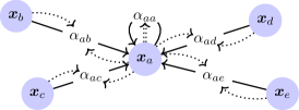
GATs are realizations of Graph Neural Networks (GNNs) operating on the concept of message-passing. In GATs, the features of the neighboring nodes are aggregated by computing attention scores α i j subscript 𝛼 𝑖 𝑗 \alpha_{ij} ( i , j ) 𝑖 𝑗 \left(i,j\right) i ∈ 𝒱 𝑖 𝒱 i\in\mathcal{V} 𝒉 i ∈ ℝ H subscript 𝒉 𝑖 superscript ℝ 𝐻 \bm{h}_{i}\in\mathbb{R}^{H} i 𝑖 i j ∈ 𝒩 i 𝑗 subscript 𝒩 𝑖 j\in\mathcal{N}_{i} i 𝑖 i 1 j ∈ 𝒩 i 𝑗 subscript 𝒩 𝑖 j\in\mathcal{N}_{i} α i j subscript 𝛼 𝑖 𝑗 \alpha_{ij}
Figure 1 : Concept of attentional message passing on graphs.[2 ]
There are different ways to compute attention scores. A very popular approach is GATv2[4 ] , where the network updates the features of node i 𝑖 i Eq. 1 3 . The equations correspond to the default implementation of GATv2 in the PyTorch Geometric framework [3 ] .
e ( 𝒉 ~ i , 𝒉 ~ j ) 𝑒 subscript ~ 𝒉 𝑖 subscript ~ 𝒉 𝑗 \displaystyle e(\tilde{\bm{h}}_{i},\tilde{\bm{h}}_{j}) = 𝒂 T LeakyReLU ( 𝚯 R 𝒉 ~ i + 𝚯 L 𝒉 ~ j ) absent superscript 𝒂 T LeakyReLU subscript 𝚯 𝑅 subscript ~ 𝒉 𝑖 subscript 𝚯 𝐿 subscript ~ 𝒉 𝑗 \displaystyle=\bm{a}^{\mathrm{T}}\text{LeakyReLU}\left({\bm{\Theta}}_{R}\tilde{\bm{h}}_{i}+{\bm{\Theta}}_{L}\tilde{\bm{h}}_{j}\right) (1)
α i j subscript 𝛼 𝑖 𝑗 \displaystyle\alpha_{ij} = softmax j ( e ( 𝒉 ~ i , 𝒉 ~ j ) ) absent subscript softmax 𝑗 𝑒 subscript bold-~ 𝒉 𝑖 subscript bold-~ 𝒉 𝑗 \displaystyle=\text{softmax}_{j}(e(\bm{\tilde{h}}_{i},\bm{\tilde{h}}_{j})) (2)
𝒉 i ′ superscript subscript 𝒉 𝑖 ′ \displaystyle\bm{h}_{i}^{\prime} = 𝒃 + ∑ j ∈ 𝒩 i α i j 𝚯 L 𝒉 ~ j absent 𝒃 subscript 𝑗 subscript 𝒩 𝑖 subscript 𝛼 𝑖 𝑗 subscript 𝚯 𝐿 subscript ~ 𝒉 𝑗 \displaystyle=\bm{b}+\sum_{j\in\mathcal{N}_{i}}\alpha_{ij}{\bm{\Theta}}_{L}\tilde{\bm{h}}_{j} (3)
The attention scores are determined by the scoring function (Eq. 1 𝒂 ∈ ℝ D 𝒂 superscript ℝ 𝐷 \bm{a}\in\mathbb{R}^{D} 𝚯 p ∈ ℝ D × ( H + 1 ) subscript 𝚯 𝑝 superscript ℝ 𝐷 𝐻 1 \bm{\Theta}_{p}\in\mathbb{R}^{D\times(H+1)} p ∈ { R , L } 𝑝 𝑅 𝐿 p\in\{R,L\} 𝒉 ~ q = [ 1 , 𝒉 q T ] T subscript ~ 𝒉 𝑞 superscript 1 superscript subscript 𝒉 𝑞 T T \tilde{\bm{h}}_{q}=[1,\bm{h}_{q}^{\mathrm{T}}]^{\mathrm{T}} q ∈ { i , j } 𝑞 𝑖 𝑗 q\in\{i,j\} 𝒉 i subscript 𝒉 𝑖 {\bm{h}}_{i} 𝒉 j subscript 𝒉 𝑗 {\bm{h}}_{j} 𝚯 R , 𝚯 L subscript 𝚯 𝑅 subscript 𝚯 𝐿
\bm{\Theta}_{R},\bm{\Theta}_{L} 𝒂 𝒂 \bm{a} j 𝑗 j e ( 𝒉 ~ i , 𝒉 ~ j ) 𝑒 subscript ~ 𝒉 𝑖 subscript ~ 𝒉 𝑗 e(\tilde{\bm{h}}_{i},\tilde{\bm{h}}_{j}) j 𝑗 j 2 ∑ j α i j = 1 subscript 𝑗 subscript 𝛼 𝑖 𝑗 1 \sum_{j}\alpha_{ij}=1 3 𝒃 ∈ ℝ D 𝒃 superscript ℝ 𝐷 \bm{b}\in\mathbb{R}^{D}
II-C Gradient computation using the Jacobian matrix
The Jacobian matrix is a matrix of all first-order partial derivatives of a vector-valued function. In the context of machine learning, the Jacobian matrix can be used to determine the gradients of the loss function with respect to the network parameters.
During forward propagation in a neural network, the output of each layer is calculated based on the input from the previous layer and layer’s parameters. Thereby, the input data is propagated through the network layer by layer to the output layer. During backpropagation, the gradients of the loss function with respect to the output of each layer are propagated backwards through the network to update the weights and biases.
To calculate the gradients of the network parameters, the Jacobian matrix of the output of each layer with respect to the input to that layer is determined. If a layer f : ℝ n → ℝ m : 𝑓 → subscript ℝ 𝑛 subscript ℝ 𝑚 f:\mathbb{R}_{n}\rightarrow\mathbb{R}_{m} 𝒚 = f ( 𝒙 ) 𝒚 𝑓 𝒙 \bm{y}=f(\bm{x}) 𝐉 𝐉 \mathbf{J} f 𝑓 f m × n 𝑚 𝑛 m\times n
𝐉 = ∂ ( vec { f ( 𝒙 ) } ) ∂ ( vec { 𝒙 } ) T = [ ∂ f ( 𝒙 ) ∂ x 1 ⋯ ∂ f ( 𝒙 ) ∂ x n ] = [ ∂ f 1 ∂ x 1 ⋯ ∂ f 1 ∂ x n ⋮ ⋱ ⋮ ∂ f m ∂ x 1 ⋯ ∂ f m ∂ x n ] , 𝐉 vec 𝑓 𝒙 superscript vec 𝒙 T matrix 𝑓 𝒙 subscript 𝑥 1 ⋯ 𝑓 𝒙 subscript 𝑥 𝑛
matrix subscript 𝑓 1 subscript 𝑥 1 ⋯ subscript 𝑓 1 subscript 𝑥 𝑛 ⋮ ⋱ ⋮ subscript 𝑓 𝑚 subscript 𝑥 1 ⋯ subscript 𝑓 𝑚 subscript 𝑥 𝑛 \mathbf{J}=\frac{\partial(\text{vec}\{f(\bm{x})\})}{\partial(\text{vec}\{\bm{x}\})^{\textrm{T}}}=\begin{bmatrix}\frac{\partial f(\bm{x})}{\partial x_{1}}\quad\cdots\quad\frac{\partial f(\bm{x})}{\partial x_{n}}\end{bmatrix}=\begin{bmatrix}\frac{\partial f_{1}}{\partial x_{1}}&\cdots&\frac{\partial f_{1}}{\partial x_{n}}\\[4.30554pt]
\vdots&\ddots&\vdots\\[4.30554pt]
\frac{\partial f_{m}}{\partial x_{1}}&\cdots&\frac{\partial f_{m}}{\partial x_{n}}\end{bmatrix}, (4)
and whose ( i , j ) 𝑖 𝑗 (i,j) 𝐉 i j = ∂ f i ∂ x j subscript 𝐉 𝑖 𝑗 subscript 𝑓 𝑖 subscript 𝑥 𝑗 \mathbf{J}_{ij}=\frac{\partial f_{i}}{\partial x_{j}} vec { 𝐗 } vec 𝐗 \text{vec}\{\mathbf{X}\} f ( 𝒙 ) 𝑓 𝒙 f(\bm{x}) y = f ( 𝒖 ) 𝑦 𝑓 𝒖 y=f(\bm{u}) 𝒖 = g ( 𝒙 ) 𝒖 𝑔 𝒙 \bm{u}=g(\bm{x})
∂ ( vec { 𝒚 } ) ∂ ( vec { 𝒙 } ) T = ∂ ( vec { 𝒚 } ) ∂ ( vec { 𝒖 } ) T ⋅ ∂ ( vec { 𝒖 } ) ∂ ( vec { 𝒙 } ) T . vec 𝒚 superscript vec 𝒙 T ⋅ vec 𝒚 superscript vec 𝒖 T vec 𝒖 superscript vec 𝒙 T \frac{\partial(\text{vec}\{\bm{y}\})}{\partial(\text{vec}\{\bm{x}\})^{\textrm{T}}}=\frac{\partial(\text{vec}\{\bm{y}\})}{\partial(\text{vec}\{\bm{u}\})^{\textrm{T}}}\cdot\frac{\partial(\text{vec}\{\bm{u}\})}{\partial(\text{vec}\{\bm{x}\})^{\textrm{T}}}. (5)
Through the repeated usage of the chain rule, the gradients of the networks’ parameters can be determined.
III Gradients of GATv2 network parameters
In this section, the derivatives for the trainable parameters of the GATv2[4 ] architecture are derived. The gradients for updating the weights and biases due to node i 𝑖 i j ∈ 𝒩 i 𝑗 subscript 𝒩 𝑖 j\in\mathcal{N}_{i} i 𝑖 i N = | 𝒩 i | 𝑁 subscript 𝒩 𝑖 N=|\mathcal{N}_{i}| 𝚯 R , 𝚯 L ∈ ℝ D × ( H + 1 ) subscript 𝚯 𝑅 subscript 𝚯 𝐿
superscript ℝ 𝐷 𝐻 1 \mathbf{\Theta}_{R},\mathbf{\Theta}_{L}\in\mathbb{R}^{D\times(H+1)} 𝒂 ∈ ℝ D 𝒂 superscript ℝ 𝐷 \bm{a}\in\mathbb{R}^{D} 𝒃 ∈ ℝ D 𝒃 superscript ℝ 𝐷 \bm{b}\in\mathbb{R}^{D} 𝚯 R = [ 𝚯 R b , 𝚯 R w ] subscript 𝚯 𝑅 subscript 𝚯 subscript 𝑅 𝑏 subscript 𝚯 subscript 𝑅 𝑤 \bm{\Theta}_{R}=[\bm{\Theta}_{R_{b}},\bm{\Theta}_{R_{w}}] 𝚯 L subscript 𝚯 𝐿 \mathbf{\Theta}_{L} 𝚯 R w subscript 𝚯 subscript 𝑅 𝑤 \bm{\Theta}_{R_{w}} 𝚯 R b subscript 𝚯 subscript 𝑅 𝑏 \bm{\Theta}_{R_{b}} ℒ ( 𝒉 i ′ , 𝒚 ) ℒ superscript subscript 𝒉 𝑖 ′ 𝒚 \mathcal{L}(\bm{h}_{i}^{\prime},\bm{y}) 2 𝚯 R subscript 𝚯 𝑅 \mathbf{\Theta}_{R} vec { 𝐗 } vec 𝐗 \text{vec}\{\mathbf{X}\} 𝐗 𝐗 \mathbf{X} c 𝑐 c
Figure 2 : Partial forward (black) and backward (blue) pass for the parameter 𝚯 R subscript 𝚯 𝑅 \mathbf{\Theta}_{R} 𝒂 l , i j subscript 𝒂 𝑙 𝑖 𝑗
\bm{a}_{l,ij} 𝒂 l , i j B superscript subscript 𝒂 𝑙 𝑖 𝑗
B {}^{\textrm{B}}\bm{a}_{l,ij} l 𝑙 l g p subscript 𝑔 𝑝 g_{p} p 𝑝 p
III-A Gradient for parameter 𝚯 R subscript 𝚯 𝑅 \mathbf{\Theta}_{R}
𝐉 a 9 , i 1 = ∂ ( vec { 𝒉 i ′ } ) ∂ ( vec { 𝒂 9 , i 1 } ) T = ∂ ( vec { ∑ j ∈ 𝒩 i 𝒂 9 , i j } ) ∂ ( vec { 𝒂 9 , i 1 } ) T = [ ∂ ( vec { ∑ j ∈ 𝒩 i a 9 , i j } ( 1 ) ) ∂ a 9 , i 1 ( 1 ) ⋯ ∂ ( vec { ∑ j ∈ 𝒩 i a 9 , i j } ( 1 ) ) ∂ a 9 , i 1 ( D ) ⋮ ⋱ ⋮ ∂ ( vec { ∑ j ∈ 𝒩 i a 9 , i j } ( D ) ) ∂ a 9 , i 1 ( 1 ) ⋯ ∂ ( vec { ∑ j ∈ 𝒩 i a 9 , i j } ( D ) ) ∂ a 9 , i 1 ( D ) ] subscript 𝐉 subscript 𝑎 9 𝑖 1
vec superscript subscript 𝒉 𝑖 ′ superscript vec subscript 𝒂 9 𝑖 1
T vec subscript 𝑗 subscript 𝒩 𝑖 subscript 𝒂 9 𝑖 𝑗
superscript vec subscript 𝒂 9 𝑖 1
T matrix vec superscript subscript 𝑗 subscript 𝒩 𝑖 subscript 𝑎 9 𝑖 𝑗
1 superscript subscript 𝑎 9 𝑖 1
1 ⋯ vec superscript subscript 𝑗 subscript 𝒩 𝑖 subscript 𝑎 9 𝑖 𝑗
1 superscript subscript 𝑎 9 𝑖 1
𝐷 ⋮ ⋱ ⋮ vec superscript subscript 𝑗 subscript 𝒩 𝑖 subscript 𝑎 9 𝑖 𝑗
𝐷 superscript subscript 𝑎 9 𝑖 1
1 ⋯ vec superscript subscript 𝑗 subscript 𝒩 𝑖 subscript 𝑎 9 𝑖 𝑗
𝐷 superscript subscript 𝑎 9 𝑖 1
𝐷 \displaystyle\mathbf{J}_{a_{9,i1}}=\frac{\partial(\text{vec}\{\bm{h}_{i}^{\prime}\})}{\partial(\text{vec}\{\bm{a}_{9,i1}\})^{\mathrm{T}}}=\frac{\partial(\text{vec}\{\sum_{j\in\mathcal{N}_{i}}\bm{a}_{9,ij}\})}{\partial(\text{vec}\{\bm{a}_{9,i1}\})^{\mathrm{T}}}=\begin{bmatrix}\frac{\partial(\text{vec}\{\sum_{j\in\mathcal{N}_{i}}a_{9,ij}\}^{(1)})}{\partial a_{9,i1}^{(1)}}&\cdots&\frac{\partial(\text{vec}\{\sum_{j\in\mathcal{N}_{i}}a_{9,ij}\}^{(1)})}{\partial a_{9,i1}^{(D)}}\\
\vdots&\ddots&\vdots\\
\frac{\partial(\text{vec}\{\sum_{j\in\mathcal{N}_{i}}a_{9,ij}\}^{(D)})}{\partial a_{9,i1}^{(1)}}&\cdots&\frac{\partial(\text{vec}\{\sum_{j\in\mathcal{N}_{i}}a_{9,ij}\}^{(D)})}{\partial a_{9,i1}^{(D)}}\\
\end{bmatrix}
= [ 1 0 ⋯ 0 0 1 ⋯ ⋮ ⋮ ⋱ ⋱ 0 0 ⋯ 0 1 ] = 𝐈 absent matrix 1 0 ⋯ 0 0 1 ⋯ ⋮ ⋮ ⋱ ⋱ 0 0 ⋯ 0 1 𝐈 \displaystyle\hskip 25.6073pt=\begin{bmatrix}1&0&\cdots&0\\
0&1&\cdots&\vdots\\
\vdots&\ddots&\ddots&0\\
0&\cdots&0&1\end{bmatrix}=\mathbf{I}
𝐉 a 8 , i 1 = 𝐉 a 9 , i 1 ⋅ ∂ ( vec { 𝒂 9 , i 1 } ) ∂ ( vec { 𝒂 8 , i 1 } ) T = 𝐉 a 9 , i 1 ⋅ ∂ ( vec { ( 𝒂 8 , i 1 ⋅ 𝒉 ~ 1 ) ) } ∂ ( vec { 𝒂 8 , i 1 } ) T = 𝐈 ⋅ [ h ~ 1 T 𝟎 1 × H ⋯ 𝟎 1 × H 𝟎 1 × H h ~ 1 T ⋯ ⋮ ⋮ ⋱ ⋱ 𝟎 1 × H 𝟎 1 × H ⋯ 𝟎 1 × H h ~ 1 T ] \displaystyle\mathbf{J}_{a_{8,i1}}=\mathbf{J}_{a_{9,i1}}\cdot\frac{\partial(\text{vec}\{\bm{a}_{9,i1}\})}{\partial(\text{vec}\{\bm{a}_{8,i1}\})^{\mathrm{T}}}=\mathbf{J}_{a_{9,i1}}\cdot\frac{\partial(\text{vec}\{({\bm{a}}_{8,i1}\cdot\tilde{\bm{h}}_{1}))\}}{\partial(\text{vec}\{\bm{a}_{8,i1}\})^{\mathrm{T}}}=\mathbf{I}\cdot\begin{bmatrix}\tilde{h}_{1}^{\textrm{T}}&\bm{0}_{1\times H}&\cdots&\bm{0}_{1\times H}\\
\bm{0}_{1\times H}&\tilde{h}_{1}^{\textrm{T}}&\cdots&\vdots\\
\vdots&\ddots&\ddots&\bm{0}_{1\times H}\\
\bm{0}_{1\times H}&\cdots&\bm{0}_{1\times H}&\tilde{h}_{1}^{\textrm{T}}\end{bmatrix}
= [ h ~ 1 T 𝟎 1 × H ⋯ 𝟎 1 × H 𝟎 1 × H h ~ 1 T ⋯ ⋮ ⋮ ⋱ ⋱ 𝟎 1 × H 𝟎 1 × H ⋯ 𝟎 1 × H h ~ 1 T ] absent matrix superscript subscript ~ ℎ 1 T subscript 0 1 𝐻 ⋯ subscript 0 1 𝐻 subscript 0 1 𝐻 superscript subscript ~ ℎ 1 T ⋯ ⋮ ⋮ ⋱ ⋱ subscript 0 1 𝐻 subscript 0 1 𝐻 ⋯ subscript 0 1 𝐻 superscript subscript ~ ℎ 1 T \displaystyle\hskip 25.6073pt=\begin{bmatrix}\tilde{h}_{1}^{\textrm{T}}&\bm{0}_{1\times H}&\cdots&\bm{0}_{1\times H}\\
\bm{0}_{1\times H}&\tilde{h}_{1}^{\textrm{T}}&\cdots&\vdots\\
\vdots&\ddots&\ddots&\bm{0}_{1\times H}\\
\bm{0}_{1\times H}&\cdots&\bm{0}_{1\times H}&\tilde{h}_{1}^{\textrm{T}}\end{bmatrix}
J a 7 , i 1 = 𝐉 a 8 , i 1 ⋅ ∂ ( vec { 𝒂 8 , i 1 } ) ∂ ( vec { a 7 , i 1 } ) T = 𝐉 a 8 , i 1 ⋅ ∂ ( vec { ( 𝚯 L ⋅ a 7 , i 1 ) } ) ∂ ( a 7 , i 1 ) T = 𝐉 a 8 , i 1 ⋅ vec { ( 𝚯 L ) } subscript 𝐽 subscript 𝑎 7 𝑖 1
⋅ subscript 𝐉 subscript 𝑎 8 𝑖 1
vec subscript 𝒂 8 𝑖 1
superscript vec subscript 𝑎 7 𝑖 1
T ⋅ subscript 𝐉 subscript 𝑎 8 𝑖 1
vec ⋅ subscript 𝚯 𝐿 subscript 𝑎 7 𝑖 1
superscript subscript 𝑎 7 𝑖 1
T ⋅ subscript 𝐉 subscript 𝑎 8 𝑖 1
vec subscript 𝚯 𝐿 \displaystyle{J}_{a_{7,i1}}=\mathbf{J}_{a_{8,i1}}\cdot\frac{\partial(\text{vec}\{\bm{a}_{8,i1}\})}{\partial(\text{vec}\{{a}_{7,i1}\})^{\textrm{T}}}=\mathbf{J}_{a_{8,i1}}\cdot\frac{\partial(\text{vec}\{(\mathbf{\Theta}_{L}\cdot{a}_{7,i1})\})}{\partial({a}_{7,i1})^{\textrm{T}}}=\mathbf{J}_{a_{8,i1}}\cdot\text{vec}\{(\mathbf{\Theta}_{L})\}
= [ 𝒉 ~ 1 T 𝟎 1 × H ⋯ 𝟎 1 × H 𝟎 1 × H 𝒉 ~ 1 T ⋯ ⋮ ⋮ ⋱ ⋱ 𝟎 1 × H 𝟎 1 × H ⋯ 𝟎 1 × H 𝒉 ~ 1 T ] ⋅ vec { ( 𝚯 L ) } = [ 𝒉 ~ 1 T 𝚯 L ( 1 ) 𝒉 ~ 1 T 𝚯 L ( 2 ) ⋮ 𝒉 ~ 1 T 𝚯 L ( D ) ] = 𝚯 L 𝒉 ~ 1 → ∑ d = 1 D ( 𝚯 L 𝒉 ~ 1 ) ( d ) absent ⋅ matrix superscript subscript ~ 𝒉 1 T subscript 0 1 𝐻 ⋯ subscript 0 1 𝐻 subscript 0 1 𝐻 superscript subscript ~ 𝒉 1 T ⋯ ⋮ ⋮ ⋱ ⋱ subscript 0 1 𝐻 subscript 0 1 𝐻 ⋯ subscript 0 1 𝐻 superscript subscript ~ 𝒉 1 T vec subscript 𝚯 𝐿 matrix superscript subscript ~ 𝒉 1 T superscript subscript 𝚯 𝐿 1 superscript subscript ~ 𝒉 1 T superscript subscript 𝚯 𝐿 2 ⋮ superscript subscript ~ 𝒉 1 T superscript subscript 𝚯 𝐿 𝐷 subscript 𝚯 𝐿 subscript ~ 𝒉 1 → superscript subscript 𝑑 1 𝐷 superscript subscript 𝚯 𝐿 subscript ~ 𝒉 1 𝑑 \displaystyle\hskip 25.6073pt=\begin{bmatrix}\tilde{\bm{h}}_{1}^{\textrm{T}}&\bm{0}_{1\times H}&\cdots&\bm{0}_{1\times H}\\
\bm{0}_{1\times H}&\tilde{\bm{h}}_{1}^{\textrm{T}}&\cdots&\vdots\\
\vdots&\ddots&\ddots&\bm{0}_{1\times H}\\
\bm{0}_{1\times H}&\cdots&\bm{0}_{1\times H}&\tilde{\bm{h}}_{1}^{\textrm{T}}\end{bmatrix}\cdot\text{vec}\{(\mathbf{\Theta}_{L})\}=\begin{bmatrix}\tilde{\bm{h}}_{1}^{\textrm{T}}\mathbf{\Theta}_{L}^{(1)}\\
\tilde{\bm{h}}_{1}^{\textrm{T}}\mathbf{\Theta}_{L}^{(2)}\\
\vdots\\
\tilde{\bm{h}}_{1}^{\textrm{T}}\mathbf{\Theta}_{L}^{(D)}\\
\end{bmatrix}=\mathbf{\Theta}_{L}\tilde{\bm{h}}_{1}\rightarrow\sum_{d=1}^{D}(\mathbf{\Theta}_{L}\tilde{\bm{h}}_{1})^{(d)}
𝐉 a 7 , i = c o n c a t j ( J a 7 , i j ) = [ J a 7 , i 1 J a 7 , i 2 ⋯ J a 7 , i N ] = [ A 7 , i 1 A 7 , i 2 ⋯ A 7 , i N ] subscript 𝐉 subscript 𝑎 7 𝑖
𝑐 𝑜 𝑛 𝑐 𝑎 subscript 𝑡 𝑗 subscript 𝐽 subscript 𝑎 7 𝑖 𝑗
subscript 𝐽 subscript 𝑎 7 𝑖 1
subscript 𝐽 subscript 𝑎 7 𝑖 2
⋯ subscript 𝐽 subscript 𝑎 7 𝑖 𝑁
matrix subscript 𝐴 7 𝑖 1
subscript 𝐴 7 𝑖 2
⋯ subscript 𝐴 7 𝑖 𝑁
\displaystyle\mathbf{J}_{a_{7,i}}=concat_{j}({J}_{a_{7,ij}})=\left[{J}_{a_{7,i1}}\quad{J}_{a_{7,i2}}\quad\cdots\quad{J}_{a_{7,iN}}\right]=\begin{bmatrix}A_{7,i1}&A_{7,i2}&\cdots&A_{7,iN}\\
\end{bmatrix}
𝐉 a 6 , i = 𝐉 a 7 , i ⋅ ∂ ( vec { 𝒂 7 , i } ) ∂ ( vec { 𝒂 6 , i } ) T = 𝐉 a 7 , i ⋅ [ ( 1 − α i 1 ) − α i 1 α i 2 − α i 1 α i 3 ⋯ − α i 1 α i N − α i 1 α i 2 α i 2 ( 1 − α i 2 ) − α i 2 α i 3 ⋯ ⋮ − α i 1 α i 3 − α i 2 α i 3 α i 3 ( 1 − α i 3 ) ⋯ ⋮ ⋮ ⋱ ⋱ ⋱ ⋮ − α i 1 α i N − α i 2 α i N ⋯ ⋯ α i N ( 1 − α i N ) ] subscript 𝐉 subscript 𝑎 6 𝑖
⋅ subscript 𝐉 subscript 𝑎 7 𝑖
vec subscript 𝒂 7 𝑖
superscript vec subscript 𝒂 6 𝑖
T ⋅ subscript 𝐉 subscript 𝑎 7 𝑖
matrix 1 subscript 𝛼 𝑖 1 subscript 𝛼 𝑖 1 subscript 𝛼 𝑖 2 subscript 𝛼 𝑖 1 subscript 𝛼 𝑖 3 ⋯ subscript 𝛼 𝑖 1 subscript 𝛼 𝑖 𝑁 subscript 𝛼 𝑖 1 subscript 𝛼 𝑖 2 subscript 𝛼 𝑖 2 1 subscript 𝛼 𝑖 2 subscript 𝛼 𝑖 2 subscript 𝛼 𝑖 3 ⋯ ⋮ subscript 𝛼 𝑖 1 subscript 𝛼 𝑖 3 subscript 𝛼 𝑖 2 subscript 𝛼 𝑖 3 subscript 𝛼 𝑖 3 1 subscript 𝛼 𝑖 3 ⋯ ⋮ ⋮ ⋱ ⋱ ⋱ ⋮ subscript 𝛼 𝑖 1 subscript 𝛼 𝑖 𝑁 subscript 𝛼 𝑖 2 subscript 𝛼 𝑖 𝑁 ⋯ ⋯ subscript 𝛼 𝑖 𝑁 1 subscript 𝛼 𝑖 𝑁 \displaystyle\mathbf{J}_{a_{6,i}}=\mathbf{J}_{a_{7,i}}\cdot\frac{\partial(\text{vec}\{\bm{a}_{7,i}\})}{\partial(\text{vec}\{\bm{a}_{6,i}\})^{\textrm{T}}}=\mathbf{J}_{a_{7,i}}\cdot\begin{bmatrix}(1-\alpha_{i1})&-\alpha_{i1}\alpha_{i2}&-\alpha_{i1}\alpha_{i3}&\cdots&-\alpha_{i1}\alpha_{iN}\\
-\alpha_{i1}\alpha_{i2}&\alpha_{i2}(1-\alpha_{i2})&-\alpha_{i2}\alpha_{i3}&\cdots&\vdots\\
-\alpha_{i1}\alpha_{i3}&-\alpha_{i2}\alpha_{i3}&\alpha_{i3}(1-\alpha_{i3})&\cdots&\vdots\\
\vdots&\ddots&\ddots&\ddots&\vdots\\
-\alpha_{i1}\alpha_{iN}&-\alpha_{i2}\alpha_{iN}&\cdots&\cdots&\alpha_{iN}(1-\alpha_{iN})\\
\end{bmatrix}
= [ ∑ j N α i 1 ( δ 1 j − α i j ) A 7 , i j ∑ j N α i 2 ( δ 2 j − α i j ) A 7 , i j ⋮ ∑ j N α i N ( δ N j − α i j ) A 7 , i j ] T , where δ l j = { 1 , if l = j 0 , else formulae-sequence absent superscript matrix superscript subscript 𝑗 𝑁 subscript 𝛼 𝑖 1 subscript 𝛿 1 𝑗 subscript 𝛼 𝑖 𝑗 subscript 𝐴 7 𝑖 𝑗
superscript subscript 𝑗 𝑁 subscript 𝛼 𝑖 2 subscript 𝛿 2 𝑗 subscript 𝛼 𝑖 𝑗 subscript 𝐴 7 𝑖 𝑗
⋮ superscript subscript 𝑗 𝑁 subscript 𝛼 𝑖 𝑁 subscript 𝛿 𝑁 𝑗 subscript 𝛼 𝑖 𝑗 subscript 𝐴 7 𝑖 𝑗
T where subscript 𝛿 𝑙 𝑗 cases 1 if 𝑙 𝑗 0 else \displaystyle\hskip 25.6073pt=\begin{bmatrix}\sum_{j}^{N}\alpha_{i1}(\delta_{1j}-\alpha_{ij})A_{7,ij}\\
\sum_{j}^{N}\alpha_{i2}(\delta_{2j}-\alpha_{ij})A_{7,ij}\\
\vdots\\
\sum_{j}^{N}\alpha_{iN}(\delta_{Nj}-\alpha_{ij})A_{7,ij}\\
\end{bmatrix}^{\textrm{T}},\quad\text{ where }\delta_{lj}=\begin{cases}1,&\text{if}\ l=j\\
0,&\text{else}\end{cases}
𝐉 a 6 , i 1 = 𝐉 a 6 , i ⋅ ∂ ( vec { 𝒂 6 , i } ) ∂ ( vec { 𝒂 6 , i 1 } ) T = 𝐉 a 6 , i 1 ⋅ [ 1 0 ⋯ 0 ] T subscript 𝐉 subscript 𝑎 6 𝑖 1
⋅ subscript 𝐉 subscript 𝑎 6 𝑖
vec subscript 𝒂 6 𝑖
superscript vec subscript 𝒂 6 𝑖 1
T ⋅ subscript 𝐉 subscript 𝑎 6 𝑖 1
superscript 1 0 ⋯ 0
T \displaystyle\mathbf{J}_{a_{6,i1}}=\mathbf{J}_{a_{6,i}}\cdot\frac{\partial(\text{vec}\{\bm{a}_{6,i}\})}{\partial(\text{vec}\{\bm{a}_{6,i1}\})^{\textrm{T}}}=\mathbf{J}_{a_{6,i1}}\cdot\left[1\quad 0\quad\cdots\quad 0\right]^{\textrm{T}}
= [ ∑ j N α i 1 ( δ 1 j − α i j ) A 7 , i j ] , where δ 1 j = { 1 , if j = 1 0 , else formulae-sequence absent matrix superscript subscript 𝑗 𝑁 subscript 𝛼 𝑖 1 subscript 𝛿 1 𝑗 subscript 𝛼 𝑖 𝑗 subscript 𝐴 7 𝑖 𝑗
where subscript 𝛿 1 𝑗 cases 1 if 𝑗 1 0 else \displaystyle\hskip 25.6073pt=\begin{bmatrix}\sum_{j}^{N}\alpha_{i1}(\delta_{1j}-\alpha_{ij})A_{7,ij}\end{bmatrix},\quad\text{ where }\delta_{1j}=\begin{cases}1,&\text{if}\ j=1\\
0,&\text{else}\end{cases}
𝐉 a 5 , i 1 = 𝐉 a 6 , i 1 ⋅ ∂ ( vec { 𝒂 6 , i 1 } ) ∂ ( vec { 𝒂 5 , i 1 } ) T = 𝐉 a 6 , i 1 ⋅ ∂ ( vec { 𝒂 5 , i 1 ⊙ 𝒂 } ) ∂ ( vec { 𝒂 5 , i 1 } ) T = 𝐉 a 6 , i 1 ⋅ [ a ( 1 ) a ( 2 ) ⋯ a ( D ) ] subscript 𝐉 subscript 𝑎 5 𝑖 1
⋅ subscript 𝐉 subscript 𝑎 6 𝑖 1
vec subscript 𝒂 6 𝑖 1
superscript vec subscript 𝒂 5 𝑖 1
T ⋅ subscript 𝐉 subscript 𝑎 6 𝑖 1
vec direct-product subscript 𝒂 5 𝑖 1
𝒂 superscript vec subscript 𝒂 5 𝑖 1
T ⋅ subscript 𝐉 subscript 𝑎 6 𝑖 1
matrix superscript 𝑎 1 superscript 𝑎 2 ⋯ superscript 𝑎 𝐷 \displaystyle\mathbf{J}_{a_{5,i1}}=\mathbf{J}_{a_{6,i1}}\cdot\frac{\partial(\text{vec}\{\bm{a}_{6,i1}\})}{\partial(\text{vec}\{\bm{a}_{5,i1}\})^{\textrm{T}}}=\mathbf{J}_{a_{6,i1}}\cdot\frac{\partial(\text{vec}\{\bm{a}_{5,i1}\odot\bm{a}\})}{\partial(\text{vec}\{\bm{a}_{5,i1}\})^{\textrm{T}}}=\mathbf{J}_{a_{6,i1}}\cdot\begin{bmatrix}{a}^{(1)}&{a}^{(2)}&\cdots&{a}^{(D)}\\
\end{bmatrix}
= [ ∑ j N α i 1 ( δ 1 j − α i j ) A 7 , i j ] ⋅ [ a ( 1 ) a ( 2 ) ⋯ a ( D ) ] absent ⋅ matrix superscript subscript 𝑗 𝑁 subscript 𝛼 𝑖 1 subscript 𝛿 1 𝑗 subscript 𝛼 𝑖 𝑗 subscript 𝐴 7 𝑖 𝑗
matrix superscript 𝑎 1 superscript 𝑎 2 ⋯ superscript 𝑎 𝐷 \displaystyle\hskip 25.6073pt=\begin{bmatrix}\sum_{j}^{N}\alpha_{i1}(\delta_{1j}-\alpha_{ij})A_{7,ij}\end{bmatrix}\cdot\begin{bmatrix}{a}^{(1)}&{a}^{(2)}&\cdots&{a}^{(D)}\\
\end{bmatrix}
= [ a ( 1 ) ∑ j N α i 1 ( δ 1 j − α i j ) A 7 , i j a ( 2 ) ∑ j N α i 1 ( δ 1 j − α i j ) A 7 , i j ⋮ a ( D ) ∑ j N α i 1 ( δ 1 j − α i j ) A 7 , i j ] T absent superscript matrix superscript 𝑎 1 superscript subscript 𝑗 𝑁 subscript 𝛼 𝑖 1 subscript 𝛿 1 𝑗 subscript 𝛼 𝑖 𝑗 subscript 𝐴 7 𝑖 𝑗
superscript 𝑎 2 superscript subscript 𝑗 𝑁 subscript 𝛼 𝑖 1 subscript 𝛿 1 𝑗 subscript 𝛼 𝑖 𝑗 subscript 𝐴 7 𝑖 𝑗
⋮ superscript 𝑎 𝐷 superscript subscript 𝑗 𝑁 subscript 𝛼 𝑖 1 subscript 𝛿 1 𝑗 subscript 𝛼 𝑖 𝑗 subscript 𝐴 7 𝑖 𝑗
T \displaystyle\hskip 25.6073pt=\begin{bmatrix}a^{(1)}\sum_{j}^{N}\alpha_{i1}(\delta_{1j}-\alpha_{ij})A_{7,ij}\\
a^{(2)}\sum_{j}^{N}\alpha_{i1}(\delta_{1j}-\alpha_{ij})A_{7,ij}\\
\vdots\\
a^{(D)}\sum_{j}^{N}\alpha_{i1}(\delta_{1j}-\alpha_{ij})A_{7,ij}\\
\end{bmatrix}^{\textrm{T}}
𝐉 a 4 , i 1 = 𝐉 a 5 , i 1 ⋅ ∂ ( vec { 𝒂 5 , i 1 } ) ∂ ( vec { 𝒂 4 , i 1 } ) T = 𝐉 a 5 , i 1 ⋅ ∂ ( LeakyRELU ( vec { 𝒂 5 , i 1 } ) ) ∂ ( vec { 𝒂 4 , i 1 } ) T = 𝐉 a 5 , i 1 ⋅ [ s i 1 ( 1 ) 0 ⋯ 0 0 s i 1 ( 2 ) ⋯ 0 ⋮ ⋱ ⋱ 0 0 0 ⋯ s i 1 ( D ) ] subscript 𝐉 subscript 𝑎 4 𝑖 1
⋅ subscript 𝐉 subscript 𝑎 5 𝑖 1
vec subscript 𝒂 5 𝑖 1
superscript vec subscript 𝒂 4 𝑖 1
T ⋅ subscript 𝐉 subscript 𝑎 5 𝑖 1
LeakyRELU vec subscript 𝒂 5 𝑖 1
superscript vec subscript 𝒂 4 𝑖 1
T ⋅ subscript 𝐉 subscript 𝑎 5 𝑖 1
matrix superscript subscript 𝑠 𝑖 1 1 0 ⋯ 0 0 superscript subscript 𝑠 𝑖 1 2 ⋯ 0 ⋮ ⋱ ⋱ 0 0 0 ⋯ superscript subscript 𝑠 𝑖 1 𝐷 \displaystyle\mathbf{J}_{a_{4,i1}}=\mathbf{J}_{a_{5,i1}}\cdot\frac{\partial(\text{vec}\{\bm{a}_{5,i1}\})}{\partial(\text{vec}\{\bm{a}_{4,i1}\})^{\textrm{T}}}=\mathbf{J}_{a_{5,i1}}\cdot\frac{\partial(\text{LeakyRELU}(\text{vec}\{\bm{a}_{5,i1}\}))}{\partial(\text{vec}\{\bm{a}_{4,i1}\})^{\textrm{T}}}=\mathbf{J}_{a_{5,i1}}\cdot\begin{bmatrix}s_{i1}^{(1)}&0&\cdots&0\\
0&s_{i1}^{(2)}&\cdots&0\\
\vdots&\ddots&\ddots&0\\
0&0&\cdots&s_{i1}^{(D)}\\
\end{bmatrix}
= [ s i 1 ( 1 ) a ( 1 ) ∑ j N ( α i 1 ( δ 1 j − α i j ) A 7 , i j ) s i 1 ( 2 ) a ( 2 ) ∑ j N ( α i 1 ( δ 1 j − α i j ) A 7 , i j ) ⋮ s i 1 ( D ) a ( D ) ∑ j N ( α i 1 ( δ 1 j − α i j ) A 7 , i j ) ] T , where s i 1 ( d ) = { 1 , if a 4 , i 1 ( d ) > 0 s n , else formulae-sequence absent superscript matrix superscript subscript 𝑠 𝑖 1 1 superscript 𝑎 1 superscript subscript 𝑗 𝑁 subscript 𝛼 𝑖 1 subscript 𝛿 1 𝑗 subscript 𝛼 𝑖 𝑗 subscript 𝐴 7 𝑖 𝑗
superscript subscript 𝑠 𝑖 1 2 superscript 𝑎 2 superscript subscript 𝑗 𝑁 subscript 𝛼 𝑖 1 subscript 𝛿 1 𝑗 subscript 𝛼 𝑖 𝑗 subscript 𝐴 7 𝑖 𝑗
⋮ superscript subscript 𝑠 𝑖 1 𝐷 superscript 𝑎 𝐷 superscript subscript 𝑗 𝑁 subscript 𝛼 𝑖 1 subscript 𝛿 1 𝑗 subscript 𝛼 𝑖 𝑗 subscript 𝐴 7 𝑖 𝑗
T where superscript subscript 𝑠 𝑖 1 𝑑 cases 1 if superscript subscript 𝑎 4 𝑖 1
𝑑 0 subscript 𝑠 𝑛 else \displaystyle\hskip 25.6073pt=\begin{bmatrix}s_{i1}^{(1)}a^{(1)}\sum_{j}^{N}(\alpha_{i1}(\delta_{1j}-\alpha_{ij})A_{7,ij})\\
s_{i1}^{(2)}a^{(2)}\sum_{j}^{N}(\alpha_{i1}(\delta_{1j}-\alpha_{ij})A_{7,ij})\\
\vdots\\
s_{i1}^{(D)}a^{(D)}\sum_{j}^{N}(\alpha_{i1}(\delta_{1j}-\alpha_{ij})A_{7,ij})\\
\end{bmatrix}^{\textrm{T}},\quad\text{ where }s_{i1}^{(d)}=\begin{cases}1,&\text{if}\ a_{4,i1}^{(d)}>0\\
s_{n},&\text{else}\end{cases}
𝐉 a 2 , i 1 = 𝐉 a 4 , i 1 ⋅ ∂ ( vec { 𝒂 4 , i 1 } ) ∂ ( vec { 𝒂 2 , i 1 } ) T = 𝐉 a 4 , i 1 ⋅ 𝐈 = 𝐉 a 4 , i 1 subscript 𝐉 subscript 𝑎 2 𝑖 1
⋅ subscript 𝐉 subscript 𝑎 4 𝑖 1
vec subscript 𝒂 4 𝑖 1
superscript vec subscript 𝒂 2 𝑖 1
T ⋅ subscript 𝐉 subscript 𝑎 4 𝑖 1
𝐈 subscript 𝐉 subscript 𝑎 4 𝑖 1
\displaystyle\mathbf{J}_{a_{2,i1}}=\mathbf{J}_{a_{4,i1}}\cdot\frac{\partial(\text{vec}\{\bm{a}_{4,i1}\})}{\partial(\text{vec}\{\bm{a}_{2,i1}\})^{\textrm{T}}}=\mathbf{J}_{a_{4,i1}}\cdot\mathbf{I}=\mathbf{J}_{a_{4,i1}}
𝚯 R w , i 1 T B = ∂ 𝒉 i ′ ∂ 𝚯 R w , i 1 = ∂ ( vec { 𝒉 i ′ } ) ∂ ( vec { 𝒂 2 , i 1 } ) T ⋅ ∂ ( vec { 𝒂 2 , i 1 } ) ∂ ( vec { 𝚯 R } ) T superscript superscript subscript 𝚯 subscript 𝑅 𝑤 𝑖 1
T B superscript subscript 𝒉 𝑖 ′ subscript 𝚯 subscript 𝑅 𝑤 𝑖 1
⋅ vec superscript subscript 𝒉 𝑖 ′ superscript vec subscript 𝒂 2 𝑖 1
T vec subscript 𝒂 2 𝑖 1
superscript vec subscript 𝚯 𝑅 T \displaystyle{}^{\text{B}}\mathbf{\Theta}_{R_{w},i1}^{\textrm{T}}=\frac{\partial\bm{h}_{i}^{\prime}}{\partial\mathbf{\Theta}_{R_{w},i1}}=\frac{\partial(\text{vec}\{\bm{h}_{i}^{\prime}\})}{\partial(\text{vec}\{\bm{a}_{2,i1}\})^{\textrm{T}}}\cdot\frac{\partial(\text{vec}\{\bm{a}_{2,i1}\})}{\partial(\text{vec}\{\mathbf{\Theta}_{R}\})^{\textrm{T}}}
= 𝐉 a 2 , i 1 ⋅ ∂ ( vec { 𝚯 R h i } ) ∂ ( vec { 𝚯 R } ) T = 𝐉 a 2 , i 1 ⋅ [ 𝒉 ~ 1 T 𝟎 1 × H ⋯ 𝟎 1 × H 𝟎 1 × H 𝒉 ~ 1 T ⋯ ⋮ ⋮ ⋱ ⋱ 𝟎 1 × H 𝟎 1 × H ⋯ 𝟎 1 × H 𝒉 ~ 1 T ] = [ h i ( 1 ) s i 1 ( 1 ) a ( 1 ) ∑ j N ( α i 1 ( δ 1 j − α i j ) A 7 , i j ) h i ( 2 ) s i 1 ( 1 ) a ( 2 ) ∑ j N ( α i 1 ( δ 1 j − α i j ) A 7 , i j ) ⋮ h i ( D ) s i 1 ( 1 ) a ( 2 ) ∑ j N ( α i 1 ( δ 1 j − α i j ) A 7 , i j ) h i ( 1 ) s i 1 ( 2 ) a ( 2 ) ∑ j N ( α i 1 ( δ 1 j − α i j ) A 7 , i j ) ⋮ h i ( D ) s i 1 ( D ) a ( 2 ) ∑ j N ( α i 1 ( δ 1 j − α i j ) A 7 , i j ) ] T absent ⋅ subscript 𝐉 subscript 𝑎 2 𝑖 1
vec subscript 𝚯 𝑅 subscript ℎ 𝑖 superscript vec subscript 𝚯 𝑅 T ⋅ subscript 𝐉 subscript 𝑎 2 𝑖 1
matrix superscript subscript ~ 𝒉 1 T subscript 0 1 𝐻 ⋯ subscript 0 1 𝐻 subscript 0 1 𝐻 superscript subscript ~ 𝒉 1 T ⋯ ⋮ ⋮ ⋱ ⋱ subscript 0 1 𝐻 subscript 0 1 𝐻 ⋯ subscript 0 1 𝐻 superscript subscript ~ 𝒉 1 T superscript matrix superscript subscript ℎ 𝑖 1 superscript subscript 𝑠 𝑖 1 1 superscript 𝑎 1 superscript subscript 𝑗 𝑁 subscript 𝛼 𝑖 1 subscript 𝛿 1 𝑗 subscript 𝛼 𝑖 𝑗 subscript 𝐴 7 𝑖 𝑗
superscript subscript ℎ 𝑖 2 superscript subscript 𝑠 𝑖 1 1 superscript 𝑎 2 superscript subscript 𝑗 𝑁 subscript 𝛼 𝑖 1 subscript 𝛿 1 𝑗 subscript 𝛼 𝑖 𝑗 subscript 𝐴 7 𝑖 𝑗
⋮ superscript subscript ℎ 𝑖 𝐷 superscript subscript 𝑠 𝑖 1 1 superscript 𝑎 2 superscript subscript 𝑗 𝑁 subscript 𝛼 𝑖 1 subscript 𝛿 1 𝑗 subscript 𝛼 𝑖 𝑗 subscript 𝐴 7 𝑖 𝑗
superscript subscript ℎ 𝑖 1 superscript subscript 𝑠 𝑖 1 2 superscript 𝑎 2 superscript subscript 𝑗 𝑁 subscript 𝛼 𝑖 1 subscript 𝛿 1 𝑗 subscript 𝛼 𝑖 𝑗 subscript 𝐴 7 𝑖 𝑗
⋮ superscript subscript ℎ 𝑖 𝐷 superscript subscript 𝑠 𝑖 1 𝐷 superscript 𝑎 2 superscript subscript 𝑗 𝑁 subscript 𝛼 𝑖 1 subscript 𝛿 1 𝑗 subscript 𝛼 𝑖 𝑗 subscript 𝐴 7 𝑖 𝑗
T \displaystyle\hskip 25.6073pt=\mathbf{J}_{a_{2,i1}}\cdot\frac{\partial(\text{vec}\{\mathbf{\Theta}_{R}h_{i}\})}{\partial(\text{vec}\{\mathbf{\Theta}_{R}\})^{\textrm{T}}}=\mathbf{J}_{a_{2,i1}}\cdot\begin{bmatrix}\!\tilde{\bm{h}}_{1}^{\textrm{T}}&\bm{0}_{1\times H}&\cdots&\bm{0}_{1\times H}\\
\bm{0}_{1\times H}&\tilde{\bm{h}}_{1}^{\textrm{T}}&\cdots&\vdots\\
\vdots&\ddots&\ddots&\bm{0}_{1\times H}\\
\bm{0}_{1\times H}&\cdots&\bm{0}_{1\times H}&\tilde{\bm{h}}_{1}^{\textrm{T}}\end{bmatrix}=\begin{bmatrix}h_{i}^{(1)}s_{i1}^{(1)}a^{(1)}\sum_{j}^{N}(\alpha_{i1}(\delta_{1j}-\alpha_{ij})A_{7,ij})\\
h_{i}^{(2)}s_{i1}^{(1)}a^{(2)}\sum_{j}^{N}(\alpha_{i1}(\delta_{1j}-\alpha_{ij})A_{7,ij})\\
\vdots\\
h_{i}^{(D)}s_{i1}^{(1)}a^{(2)}\sum_{j}^{N}(\alpha_{i1}(\delta_{1j}-\alpha_{ij})A_{7,ij})\\
h_{i}^{(1)}s_{i1}^{(2)}a^{(2)}\sum_{j}^{N}(\alpha_{i1}(\delta_{1j}-\alpha_{ij})A_{7,ij})\\
\vdots\\
h_{i}^{(D)}s_{i1}^{(D)}a^{(2)}\sum_{j}^{N}(\alpha_{i1}(\delta_{1j}-\alpha_{ij})A_{7,ij})\\
\end{bmatrix}^{\textrm{T}}
= [ h i ( 1 ) s i 1 ( 1 ) a ( 1 ) α i 1 ∑ j N ( ( δ 1 j − α i j ) A 7 , i j ) h i ( 2 ) s i 1 ( 1 ) a ( 2 ) α i 1 ∑ j N ( ( δ 1 j − α i j ) A 7 , i j ) ⋮ h i ( D ) s i 1 ( 1 ) a ( 2 ) α i 1 ∑ j N ( ( δ 1 j − α i j ) A 7 , i j ) h i ( 1 ) s i 1 ( 2 ) a ( 2 ) α i 1 ∑ j N ( ( δ 1 j − α i j ) A 7 , i j ) ⋮ h i ( D ) s i 1 ( D ) a ( 2 ) α i 1 ∑ j N ( ( δ 1 j − α i j ) A 7 , i j ) ] T = [ h i ( 1 ) s i 1 ( 1 ) a ( 1 ) α i 1 S 1 h i ( 2 ) s i 1 ( 1 ) a ( 2 ) α i 1 S 1 ⋮ h i ( D ) s i 1 ( 1 ) a ( 2 ) α i 1 S 1 h i ( 1 ) s i 1 ( 2 ) a ( 2 ) α i 1 S 1 ⋮ h i ( D ) s i 1 ( D ) a ( 2 ) α i 1 S 1 ] T absent superscript matrix superscript subscript ℎ 𝑖 1 superscript subscript 𝑠 𝑖 1 1 superscript 𝑎 1 subscript 𝛼 𝑖 1 superscript subscript 𝑗 𝑁 subscript 𝛿 1 𝑗 subscript 𝛼 𝑖 𝑗 subscript 𝐴 7 𝑖 𝑗
superscript subscript ℎ 𝑖 2 superscript subscript 𝑠 𝑖 1 1 superscript 𝑎 2 subscript 𝛼 𝑖 1 superscript subscript 𝑗 𝑁 subscript 𝛿 1 𝑗 subscript 𝛼 𝑖 𝑗 subscript 𝐴 7 𝑖 𝑗
⋮ superscript subscript ℎ 𝑖 𝐷 superscript subscript 𝑠 𝑖 1 1 superscript 𝑎 2 subscript 𝛼 𝑖 1 superscript subscript 𝑗 𝑁 subscript 𝛿 1 𝑗 subscript 𝛼 𝑖 𝑗 subscript 𝐴 7 𝑖 𝑗
superscript subscript ℎ 𝑖 1 superscript subscript 𝑠 𝑖 1 2 superscript 𝑎 2 subscript 𝛼 𝑖 1 superscript subscript 𝑗 𝑁 subscript 𝛿 1 𝑗 subscript 𝛼 𝑖 𝑗 subscript 𝐴 7 𝑖 𝑗
⋮ superscript subscript ℎ 𝑖 𝐷 superscript subscript 𝑠 𝑖 1 𝐷 superscript 𝑎 2 subscript 𝛼 𝑖 1 superscript subscript 𝑗 𝑁 subscript 𝛿 1 𝑗 subscript 𝛼 𝑖 𝑗 subscript 𝐴 7 𝑖 𝑗
T superscript matrix superscript subscript ℎ 𝑖 1 superscript subscript 𝑠 𝑖 1 1 superscript 𝑎 1 subscript 𝛼 𝑖 1 subscript 𝑆 1 superscript subscript ℎ 𝑖 2 superscript subscript 𝑠 𝑖 1 1 superscript 𝑎 2 subscript 𝛼 𝑖 1 subscript 𝑆 1 ⋮ superscript subscript ℎ 𝑖 𝐷 superscript subscript 𝑠 𝑖 1 1 superscript 𝑎 2 subscript 𝛼 𝑖 1 subscript 𝑆 1 superscript subscript ℎ 𝑖 1 superscript subscript 𝑠 𝑖 1 2 superscript 𝑎 2 subscript 𝛼 𝑖 1 subscript 𝑆 1 ⋮ superscript subscript ℎ 𝑖 𝐷 superscript subscript 𝑠 𝑖 1 𝐷 superscript 𝑎 2 subscript 𝛼 𝑖 1 subscript 𝑆 1 T \displaystyle\hskip 25.6073pt=\begin{bmatrix}h_{i}^{(1)}s_{i1}^{(1)}a^{(1)}\alpha_{i1}\sum_{j}^{N}((\delta_{1j}-\alpha_{ij})A_{7,ij})\\
h_{i}^{(2)}s_{i1}^{(1)}a^{(2)}\alpha_{i1}\sum_{j}^{N}((\delta_{1j}-\alpha_{ij})A_{7,ij})\\
\vdots\\
h_{i}^{(D)}s_{i1}^{(1)}a^{(2)}\alpha_{i1}\sum_{j}^{N}((\delta_{1j}-\alpha_{ij})A_{7,ij})\\
h_{i}^{(1)}s_{i1}^{(2)}a^{(2)}\alpha_{i1}\sum_{j}^{N}((\delta_{1j}-\alpha_{ij})A_{7,ij})\\
\vdots\\
h_{i}^{(D)}s_{i1}^{(D)}a^{(2)}\alpha_{i1}\sum_{j}^{N}((\delta_{1j}-\alpha_{ij})A_{7,ij})\\
\end{bmatrix}^{\textrm{T}}=\begin{bmatrix}h_{i}^{(1)}s_{i1}^{(1)}a^{(1)}\alpha_{i1}S_{1}\\
h_{i}^{(2)}s_{i1}^{(1)}a^{(2)}\alpha_{i1}S_{1}\\
\vdots\\
h_{i}^{(D)}s_{i1}^{(1)}a^{(2)}\alpha_{i1}S_{1}\\
h_{i}^{(1)}s_{i1}^{(2)}a^{(2)}\alpha_{i1}S_{1}\\
\vdots\\
h_{i}^{(D)}s_{i1}^{(D)}a^{(2)}\alpha_{i1}S_{1}\\
\end{bmatrix}^{\textrm{T}}
𝚯 R w , i T B = ∂ 𝒉 i ′ ∂ 𝚯 R w , i = ∑ k N 𝚯 R w , i k T B = ∑ k N [ h i ( 1 ) s i k ( 1 ) a ( 1 ) α i k S k ⋮ h i ( D ) s i k ( D ) a ( D ) α i k S k ] T superscript superscript subscript 𝚯 subscript 𝑅 𝑤 𝑖
T B superscript subscript 𝒉 𝑖 ′ subscript 𝚯 subscript 𝑅 𝑤 𝑖
superscript subscript 𝑘 𝑁 superscript superscript subscript 𝚯 subscript 𝑅 𝑤 𝑖 𝑘
T B superscript subscript 𝑘 𝑁 superscript matrix superscript subscript ℎ 𝑖 1 superscript subscript 𝑠 𝑖 𝑘 1 superscript 𝑎 1 subscript 𝛼 𝑖 𝑘 subscript 𝑆 𝑘 ⋮ superscript subscript ℎ 𝑖 𝐷 superscript subscript 𝑠 𝑖 𝑘 𝐷 superscript 𝑎 𝐷 subscript 𝛼 𝑖 𝑘 subscript 𝑆 𝑘 T \displaystyle{}^{\text{B}}\mathbf{\Theta}_{R_{w},i}^{\textrm{T}}=\frac{\partial\bm{h}_{i}^{\prime}}{\partial\mathbf{\Theta}_{R_{w},i}}=\sum_{k}^{N}{}^{\text{B}}\mathbf{\Theta}_{R_{w},ik}^{\textrm{T}}=\sum_{k}^{N}\begin{bmatrix}h_{i}^{(1)}s_{ik}^{(1)}a^{(1)}\alpha_{ik}S_{k}\\
\vdots\\
h_{i}^{(D)}s_{ik}^{(D)}a^{(D)}\alpha_{ik}S_{k}\\
\end{bmatrix}^{\textrm{T}}
Hence, the gradient of 𝒉 i ′ superscript subscript 𝒉 𝑖 ′ \bm{h}_{i}^{\prime} t 𝑡 t 𝚯 R w , i subscript 𝚯 subscript 𝑅 𝑤 𝑖
\mathbf{\Theta}_{R_{w,i}}
Θ R w , i ( t ) B = ∑ k N Θ R w , i k ( t ) B = ∑ k N [ h i ( t ) a ( t ) s i k ( t ) α i k S k ] = h i ( t ) a ( t ) ∑ k N [ s i k ( t ) α i k S k ] superscript superscript subscript Θ subscript 𝑅 𝑤 𝑖
𝑡 B superscript subscript 𝑘 𝑁 superscript superscript subscript Θ subscript 𝑅 𝑤 𝑖 𝑘
𝑡 B superscript subscript 𝑘 𝑁 matrix superscript subscript ℎ 𝑖 𝑡 superscript 𝑎 𝑡 superscript subscript 𝑠 𝑖 𝑘 𝑡 subscript 𝛼 𝑖 𝑘 subscript 𝑆 𝑘 superscript subscript ℎ 𝑖 𝑡 superscript 𝑎 𝑡 superscript subscript 𝑘 𝑁 matrix superscript subscript 𝑠 𝑖 𝑘 𝑡 subscript 𝛼 𝑖 𝑘 subscript 𝑆 𝑘 \displaystyle{}^{\text{B}}{\Theta}_{R_{w},i}^{(t)}=\sum_{k}^{N}{}^{\text{B}}{\Theta}_{R_{w},ik}^{(t)}=\sum_{k}^{N}\begin{bmatrix}h_{i}^{(t)}a^{(t)}s_{ik}^{(t)}\alpha_{ik}S_{k}\end{bmatrix}=h_{i}^{(t)}a^{(t)}\sum_{k}^{N}\begin{bmatrix}s_{ik}^{(t)}\alpha_{ik}S_{k}\end{bmatrix}
where S k = ∑ j N ( δ k j − α i j ) A 7 , i j , with δ k j = { 1 , if k = j 0 , else formulae-sequence where subscript 𝑆 𝑘 superscript subscript 𝑗 𝑁 subscript 𝛿 𝑘 𝑗 subscript 𝛼 𝑖 𝑗 subscript 𝐴 7 𝑖 𝑗
with subscript 𝛿 𝑘 𝑗 cases 1 if 𝑘 𝑗 0 else \displaystyle\hskip 25.6073pt\text{ where }S_{k}=\sum_{j}^{N}(\delta_{kj}-\alpha_{ij})A_{7,ij},\quad\text{ with }\delta_{kj}=\begin{cases}1,&\text{if}\ k=j\\
0,&\text{else}\end{cases}
and A 7 , i j = ∑ d D ( 𝚯 L 𝒉 ~ j ) ( d ) . and subscript 𝐴 7 𝑖 𝑗
superscript subscript 𝑑 𝐷 superscript subscript 𝚯 𝐿 subscript ~ 𝒉 𝑗 𝑑 \displaystyle\hskip 25.6073pt\text{ and }A_{7,ij}=\sum_{d}^{D}\left(\mathbf{\Theta}_{L}\tilde{\bm{h}}_{j}\right)^{(d)}.
The mathematical expression can be reformulated as follows.
Θ R w , i ( t ) B = h i ( t ) a ( t ) ∑ k N [ s i k ( t ) α i k S k ] = h i ( t ) a ( t ) ∑ k N [ s i k ( t ) α i k ∑ j N ( δ k j − α i j ) A 7 , i j ] superscript superscript subscript Θ subscript 𝑅 𝑤 𝑖
𝑡 B superscript subscript ℎ 𝑖 𝑡 superscript 𝑎 𝑡 superscript subscript 𝑘 𝑁 matrix superscript subscript 𝑠 𝑖 𝑘 𝑡 subscript 𝛼 𝑖 𝑘 subscript 𝑆 𝑘 superscript subscript ℎ 𝑖 𝑡 superscript 𝑎 𝑡 superscript subscript 𝑘 𝑁 matrix superscript subscript 𝑠 𝑖 𝑘 𝑡 subscript 𝛼 𝑖 𝑘 superscript subscript 𝑗 𝑁 subscript 𝛿 𝑘 𝑗 subscript 𝛼 𝑖 𝑗 subscript 𝐴 7 𝑖 𝑗
\displaystyle{}^{\text{B}}{\Theta}_{R_{w},i}^{(t)}=h_{i}^{(t)}a^{(t)}\sum_{k}^{N}\begin{bmatrix}s_{ik}^{(t)}\alpha_{ik}S_{k}\end{bmatrix}=h_{i}^{(t)}a^{(t)}\sum_{k}^{N}\begin{bmatrix}s_{ik}^{(t)}\alpha_{ik}\sum\limits_{j}^{N}(\delta_{kj}-\alpha_{ij})A_{7,ij}\end{bmatrix}
= h i ( t ) a ( t ) ∑ k N [ s i k ( t ) α i k ( ∑ j ≠ k N ( − α i j ) A 7 , i j + ( 1 − α i k ) A 7 , i k ) ] , where α i k = ( 1 − ∑ j ≠ k N α i j ) formulae-sequence absent superscript subscript ℎ 𝑖 𝑡 superscript 𝑎 𝑡 superscript subscript 𝑘 𝑁 matrix superscript subscript 𝑠 𝑖 𝑘 𝑡 subscript 𝛼 𝑖 𝑘 superscript subscript 𝑗 𝑘 𝑁 subscript 𝛼 𝑖 𝑗 subscript 𝐴 7 𝑖 𝑗
1 subscript 𝛼 𝑖 𝑘 subscript 𝐴 7 𝑖 𝑘
where subscript 𝛼 𝑖 𝑘 1 superscript subscript 𝑗 𝑘 𝑁 subscript 𝛼 𝑖 𝑗 \displaystyle\hskip 25.6073pt=h_{i}^{(t)}a^{(t)}\sum_{k}^{N}\begin{bmatrix}s_{ik}^{(t)}\alpha_{ik}\left(\sum\limits_{j\neq k}^{N}(-\alpha_{ij})A_{7,ij}+(1-\alpha_{ik})A_{7,ik}\right)\end{bmatrix},\quad\text{ where }\alpha_{ik}=(1-\sum\limits_{j\neq k}^{N}\alpha_{ij})
= h i ( t ) a ( t ) ∑ k N [ s i k ( t ) α i k ( ∑ j ≠ k N ( − α i j ) A 7 , i j + ( 1 − ( 1 − ∑ j ≠ k N α i j ) ) A 7 , i k ) ] absent superscript subscript ℎ 𝑖 𝑡 superscript 𝑎 𝑡 superscript subscript 𝑘 𝑁 matrix superscript subscript 𝑠 𝑖 𝑘 𝑡 subscript 𝛼 𝑖 𝑘 superscript subscript 𝑗 𝑘 𝑁 subscript 𝛼 𝑖 𝑗 subscript 𝐴 7 𝑖 𝑗
1 1 superscript subscript 𝑗 𝑘 𝑁 subscript 𝛼 𝑖 𝑗 subscript 𝐴 7 𝑖 𝑘
\displaystyle\hskip 25.6073pt=h_{i}^{(t)}a^{(t)}\sum_{k}^{N}\begin{bmatrix}s_{ik}^{(t)}\alpha_{ik}\left(\sum\limits_{j\neq k}^{N}(-\alpha_{ij})A_{7,ij}+(1-(1-\sum_{j\neq k}^{N}\alpha_{ij}))A_{7,ik}\right)\end{bmatrix}
= h i ( t ) a ( t ) ∑ k N [ s i k ( t ) α i k ( ∑ j ≠ k N ( − α i j ) A 7 , i j + ( ∑ j ≠ k N α i j ) A 7 , i k ) ] absent superscript subscript ℎ 𝑖 𝑡 superscript 𝑎 𝑡 superscript subscript 𝑘 𝑁 matrix superscript subscript 𝑠 𝑖 𝑘 𝑡 subscript 𝛼 𝑖 𝑘 superscript subscript 𝑗 𝑘 𝑁 subscript 𝛼 𝑖 𝑗 subscript 𝐴 7 𝑖 𝑗
superscript subscript 𝑗 𝑘 𝑁 subscript 𝛼 𝑖 𝑗 subscript 𝐴 7 𝑖 𝑘
\displaystyle\hskip 25.6073pt=h_{i}^{(t)}a^{(t)}\sum_{k}^{N}\begin{bmatrix}s_{ik}^{(t)}\alpha_{ik}\left(\sum\limits_{j\neq k}^{N}(-\alpha_{ij})A_{7,ij}+(\sum\limits_{j\neq k}^{N}\alpha_{ij})A_{7,ik}\right)\end{bmatrix}
= h i ( t ) a ( t ) ∑ k N [ s i k ( t ) ( ∑ j ≠ k N α i k α i j ( A 7 , i k − A 7 , i j ) ) ] absent superscript subscript ℎ 𝑖 𝑡 superscript 𝑎 𝑡 superscript subscript 𝑘 𝑁 matrix superscript subscript 𝑠 𝑖 𝑘 𝑡 superscript subscript 𝑗 𝑘 𝑁 subscript 𝛼 𝑖 𝑘 subscript 𝛼 𝑖 𝑗 subscript 𝐴 7 𝑖 𝑘
subscript 𝐴 7 𝑖 𝑗
\displaystyle\hskip 25.6073pt=h_{i}^{(t)}a^{(t)}\sum_{k}^{N}\begin{bmatrix}s_{ik}^{(t)}\left(\sum\limits_{j\neq k}^{N}\alpha_{ik}\alpha_{ij}(A_{7,ik}-A_{7,ij})\right)\end{bmatrix}
= h i ( t ) a ( t ) ∑ k N ∑ j ≠ k N [ s i k ( t ) α i k α i j ( A 7 , i k − A 7 , i j ) ] absent superscript subscript ℎ 𝑖 𝑡 superscript 𝑎 𝑡 superscript subscript 𝑘 𝑁 superscript subscript 𝑗 𝑘 𝑁 matrix superscript subscript 𝑠 𝑖 𝑘 𝑡 subscript 𝛼 𝑖 𝑘 subscript 𝛼 𝑖 𝑗 subscript 𝐴 7 𝑖 𝑘
subscript 𝐴 7 𝑖 𝑗
\displaystyle\hskip 25.6073pt=h_{i}^{(t)}a^{(t)}\sum_{k}^{N}\sum\limits_{j\neq k}^{N}\begin{bmatrix}s_{ik}^{(t)}\alpha_{ik}\alpha_{ij}(A_{7,ik}-A_{7,ij})\end{bmatrix}
= h i ( t ) a ( t ) ∑ k N ∑ j ≠ k N 1 2 [ 2 s i k ( t ) α i k α i j ( A 7 , i k − A 7 , i j ) ] absent superscript subscript ℎ 𝑖 𝑡 superscript 𝑎 𝑡 superscript subscript 𝑘 𝑁 superscript subscript 𝑗 𝑘 𝑁 1 2 matrix 2 superscript subscript 𝑠 𝑖 𝑘 𝑡 subscript 𝛼 𝑖 𝑘 subscript 𝛼 𝑖 𝑗 subscript 𝐴 7 𝑖 𝑘
subscript 𝐴 7 𝑖 𝑗
\displaystyle\hskip 25.6073pt=h_{i}^{(t)}a^{(t)}\sum_{k}^{N}\sum\limits_{j\neq k}^{N}\frac{1}{2}\begin{bmatrix}2\,s_{ik}^{(t)}\alpha_{ik}\alpha_{ij}(A_{7,ik}-A_{7,ij})\end{bmatrix}
= h i ( t ) a ( t ) ∑ k N ∑ j ≠ k N 1 2 [ s i k ( t ) α i k α i j ( A 7 , i k − A 7 , i j ) + s i k ( t ) α i k α i j ( A 7 , i k − A 7 , i j ) ] absent superscript subscript ℎ 𝑖 𝑡 superscript 𝑎 𝑡 superscript subscript 𝑘 𝑁 superscript subscript 𝑗 𝑘 𝑁 1 2 matrix superscript subscript 𝑠 𝑖 𝑘 𝑡 subscript 𝛼 𝑖 𝑘 subscript 𝛼 𝑖 𝑗 subscript 𝐴 7 𝑖 𝑘
subscript 𝐴 7 𝑖 𝑗
superscript subscript 𝑠 𝑖 𝑘 𝑡 subscript 𝛼 𝑖 𝑘 subscript 𝛼 𝑖 𝑗 subscript 𝐴 7 𝑖 𝑘
subscript 𝐴 7 𝑖 𝑗
\displaystyle\hskip 25.6073pt=h_{i}^{(t)}a^{(t)}\sum_{k}^{N}\sum_{j\neq k}^{N}\frac{1}{2}\begin{bmatrix}s_{ik}^{(t)}\alpha_{ik}\alpha_{ij}(A_{7,ik}-A_{7,ij})+s_{ik}^{(t)}\alpha_{ik}\alpha_{ij}(A_{7,ik}-A_{7,ij})\end{bmatrix}
= h i ( t ) a ( t ) ( ∑ k N ∑ j ≠ k N 1 2 [ s i k ( t ) α i k α i j ( A 7 , i k − A 7 , i j ) ] + ∑ k N ∑ j ≠ k N 1 2 [ s i k ( t ) α i k α i j ( A 7 , i k − A 7 , i j ) ] ) absent superscript subscript ℎ 𝑖 𝑡 superscript 𝑎 𝑡 superscript subscript 𝑘 𝑁 superscript subscript 𝑗 𝑘 𝑁 1 2 matrix superscript subscript 𝑠 𝑖 𝑘 𝑡 subscript 𝛼 𝑖 𝑘 subscript 𝛼 𝑖 𝑗 subscript 𝐴 7 𝑖 𝑘
subscript 𝐴 7 𝑖 𝑗
superscript subscript 𝑘 𝑁 superscript subscript 𝑗 𝑘 𝑁 1 2 matrix superscript subscript 𝑠 𝑖 𝑘 𝑡 subscript 𝛼 𝑖 𝑘 subscript 𝛼 𝑖 𝑗 subscript 𝐴 7 𝑖 𝑘
subscript 𝐴 7 𝑖 𝑗
\displaystyle\hskip 25.6073pt=h_{i}^{(t)}a^{(t)}\left(\sum_{k}^{N}\sum_{j\neq k}^{N}\frac{1}{2}\begin{bmatrix}s_{ik}^{(t)}\alpha_{ik}\alpha_{ij}(A_{7,ik}-A_{7,ij})\end{bmatrix}+\sum_{k}^{N}\sum_{j\neq k}^{N}\frac{1}{2}\begin{bmatrix}s_{ik}^{(t)}\alpha_{ik}\alpha_{ij}(A_{7,ik}-A_{7,ij})\end{bmatrix}\right)
= h i ( t ) a ( t ) ( ∑ k N ∑ j ≠ k N 1 2 [ s i k ( t ) α i k α i j ( A 7 , i k − A 7 , i j ) ] − ∑ k N ∑ j ≠ k N 1 2 [ s i k ( t ) α i k α i j ( A 7 , i j − A 7 , i k ) ] ) absent superscript subscript ℎ 𝑖 𝑡 superscript 𝑎 𝑡 superscript subscript 𝑘 𝑁 superscript subscript 𝑗 𝑘 𝑁 1 2 matrix superscript subscript 𝑠 𝑖 𝑘 𝑡 subscript 𝛼 𝑖 𝑘 subscript 𝛼 𝑖 𝑗 subscript 𝐴 7 𝑖 𝑘
subscript 𝐴 7 𝑖 𝑗
superscript subscript 𝑘 𝑁 superscript subscript 𝑗 𝑘 𝑁 1 2 matrix superscript subscript 𝑠 𝑖 𝑘 𝑡 subscript 𝛼 𝑖 𝑘 subscript 𝛼 𝑖 𝑗 subscript 𝐴 7 𝑖 𝑗
subscript 𝐴 7 𝑖 𝑘
\displaystyle\hskip 25.6073pt=h_{i}^{(t)}a^{(t)}\left(\sum_{k}^{N}\sum_{j\neq k}^{N}\frac{1}{2}\begin{bmatrix}s_{ik}^{(t)}\alpha_{ik}\alpha_{ij}(A_{7,ik}-A_{7,ij})\end{bmatrix}-\sum_{k}^{N}\sum_{j\neq k}^{N}\frac{1}{2}\begin{bmatrix}s_{ik}^{(t)}\alpha_{ik}\alpha_{ij}(A_{7,ij}-A_{7,ik})\end{bmatrix}\right)
= h i ( t ) a ( t ) ( ∑ k N ∑ j ≠ k N 1 2 [ s i k ( t ) α i k α i j ( A 7 , i k − A 7 , i j ) ] − ∑ j N ∑ k ≠ j N 1 2 [ s i j ( t ) α i k α i j ( A 7 , i k − A 7 , i j ) ] ) absent superscript subscript ℎ 𝑖 𝑡 superscript 𝑎 𝑡 superscript subscript 𝑘 𝑁 superscript subscript 𝑗 𝑘 𝑁 1 2 matrix superscript subscript 𝑠 𝑖 𝑘 𝑡 subscript 𝛼 𝑖 𝑘 subscript 𝛼 𝑖 𝑗 subscript 𝐴 7 𝑖 𝑘
subscript 𝐴 7 𝑖 𝑗
superscript subscript 𝑗 𝑁 superscript subscript 𝑘 𝑗 𝑁 1 2 matrix superscript subscript 𝑠 𝑖 𝑗 𝑡 subscript 𝛼 𝑖 𝑘 subscript 𝛼 𝑖 𝑗 subscript 𝐴 7 𝑖 𝑘
subscript 𝐴 7 𝑖 𝑗
\displaystyle\hskip 25.6073pt=h_{i}^{(t)}a^{(t)}\left(\sum_{k}^{N}\sum_{j\neq k}^{N}\frac{1}{2}\begin{bmatrix}s_{ik}^{(t)}\alpha_{ik}\alpha_{ij}(A_{7,ik}-A_{7,ij})\end{bmatrix}-\sum_{j}^{N}\sum_{k\neq j}^{N}\frac{1}{2}\begin{bmatrix}s_{ij}^{(t)}\alpha_{ik}\alpha_{ij}(A_{7,ik}-A_{7,ij})\end{bmatrix}\right)
= h i ( t ) a ( t ) ∑ k N ∑ j N 1 2 [ α i k α i j ( A 7 , i k − A 7 , i j ) ( s i k ( t ) − s i j ( t ) ) ] , j ≠ k formulae-sequence absent superscript subscript ℎ 𝑖 𝑡 superscript 𝑎 𝑡 superscript subscript 𝑘 𝑁 superscript subscript 𝑗 𝑁 1 2 matrix subscript 𝛼 𝑖 𝑘 subscript 𝛼 𝑖 𝑗 subscript 𝐴 7 𝑖 𝑘
subscript 𝐴 7 𝑖 𝑗
superscript subscript 𝑠 𝑖 𝑘 𝑡 superscript subscript 𝑠 𝑖 𝑗 𝑡 𝑗 𝑘 \displaystyle\hskip 25.6073pt=h_{i}^{(t)}a^{(t)}\sum_{k}^{N}\sum_{j}^{N}\frac{1}{2}\begin{bmatrix}\alpha_{ik}\alpha_{ij}(A_{7,ik}-A_{7,ij})(s_{ik}^{(t)}-s_{ij}^{(t)})\end{bmatrix},\quad j\neq k
= h i ( t ) a ( t ) ∑ j , k 𝒮 i [ α i k α i j ( A 7 , i k − A 7 , i j ) ( s i k ( t ) − s i j ( t ) ) ] , absent superscript subscript ℎ 𝑖 𝑡 superscript 𝑎 𝑡 superscript subscript 𝑗 𝑘
subscript 𝒮 𝑖 matrix subscript 𝛼 𝑖 𝑘 subscript 𝛼 𝑖 𝑗 subscript 𝐴 7 𝑖 𝑘
subscript 𝐴 7 𝑖 𝑗
superscript subscript 𝑠 𝑖 𝑘 𝑡 superscript subscript 𝑠 𝑖 𝑗 𝑡 \displaystyle\hskip 25.6073pt=h_{i}^{(t)}a^{(t)}\sum_{j,k}^{\mathcal{S}_{i}}\begin{bmatrix}\alpha_{ik}\alpha_{ij}(A_{7,ik}-A_{7,ij})(s_{ik}^{(t)}-s_{ij}^{(t)})\end{bmatrix},
where 𝒮 i = [ 𝒩 i ] 2 subscript 𝒮 𝑖 superscript delimited-[] subscript 𝒩 𝑖 2 \mathcal{S}_{i}=[\mathcal{N}_{i}]^{2} 𝒩 i subscript 𝒩 𝑖 \mathcal{N}_{i}
With regard to the loss function ℒ ℒ \mathcal{L} Θ R w , i ( t ) superscript subscript Θ subscript 𝑅 𝑤 𝑖
𝑡 {\Theta}_{R_{w,i}}^{(t)} Θ R w , i ( t ) superscript subscript Θ subscript 𝑅 𝑤 𝑖
𝑡 {\Theta}_{R_{w,i}}^{(t)}
Θ R w , i ( t ) B = ∂ ℒ ∂ h i ′ ( t ) ⋅ [ h i ( t ) a ( t ) ∑ j , k 𝒮 i α i j α i k ( A j − A k ) ( s i j ( t ) − s i k ( t ) ) ] , and superscript superscript subscript Θ subscript 𝑅 𝑤 𝑖
𝑡 B ⋅ ℒ superscript subscript ℎ 𝑖 ′ 𝑡
delimited-[] superscript subscript ℎ 𝑖 𝑡 superscript 𝑎 𝑡 superscript subscript 𝑗 𝑘
subscript 𝒮 𝑖 subscript 𝛼 𝑖 𝑗 subscript 𝛼 𝑖 𝑘 subscript 𝐴 𝑗 subscript 𝐴 𝑘 superscript subscript 𝑠 𝑖 𝑗 𝑡 superscript subscript 𝑠 𝑖 𝑘 𝑡 and
\displaystyle{}^{\text{B}}\Theta_{R_{w},i}^{(t)}=\frac{\partial\mathcal{L}}{\partial{h}_{i}^{\prime(t)}}\!\cdot\!\left[h_{i}^{(t)}a^{(t)}\sum_{j,k}^{\mathcal{S}_{i}}\alpha_{ij}\alpha_{ik}(A_{j}\!-\!A_{k})(s_{ij}^{(t)}-s_{ik}^{(t)})\right]\!,\quad\text{and}
Θ R b , i ( t ) B = ∂ ℒ ∂ h i ′ ( t ) ⋅ [ a ( t ) ∑ j , k 𝒮 i α i j α i k ( A j − A k ) ( s i j ( t ) − s i k ( t ) ) ] , superscript superscript subscript Θ subscript 𝑅 𝑏 𝑖
𝑡 B ⋅ ℒ superscript subscript ℎ 𝑖 ′ 𝑡
delimited-[] superscript 𝑎 𝑡 superscript subscript 𝑗 𝑘
subscript 𝒮 𝑖 subscript 𝛼 𝑖 𝑗 subscript 𝛼 𝑖 𝑘 subscript 𝐴 𝑗 subscript 𝐴 𝑘 superscript subscript 𝑠 𝑖 𝑗 𝑡 superscript subscript 𝑠 𝑖 𝑘 𝑡 \displaystyle{}^{\text{B}}\Theta_{R_{b},i}^{(t)}=\frac{\partial\mathcal{L}}{\partial{h}_{i}^{\prime(t)}}\!\cdot\!\left[a^{(t)}\sum_{j,k}^{\mathcal{S}_{i}}\alpha_{ij}\alpha_{ik}(A_{j}\!-\!A_{k})(s_{ij}^{(t)}-s_{ik}^{(t)})\right]\!,
where s i { j , k } ( t ) = { 1 , if a 4 , i { j , k } ( t ) > 0 s n , else , where superscript subscript 𝑠 𝑖 𝑗 𝑘 𝑡 cases 1 if superscript subscript 𝑎 4 𝑖 𝑗 𝑘
𝑡 0 subscript 𝑠 𝑛 else \displaystyle\hskip 25.6073pt\text{ where }s_{i\{j,k\}}^{(t)}=\begin{cases}1,&\text{if}\ a_{4,i\{j,k\}}^{(t)}>0\\
s_{n},&\text{else}\end{cases},
and A 7 , i j = ∑ d D ( 𝚯 L 𝒉 ~ j ) ( d ) . and subscript 𝐴 7 𝑖 𝑗
superscript subscript 𝑑 𝐷 superscript subscript 𝚯 𝐿 subscript ~ 𝒉 𝑗 𝑑 \displaystyle\hskip 25.6073pt\text{ and }A_{7,ij}=\sum_{d}^{D}\left(\mathbf{\Theta}_{L}\tilde{\bm{h}}_{j}\right)^{(d)}.
III-B Gradient for parameter 𝚯 L subscript 𝚯 𝐿 \mathbf{\Theta}_{L}
With regard to the loss function ℒ ℒ \mathcal{L} Θ L w , i ( t ) superscript subscript Θ subscript 𝐿 𝑤 𝑖
𝑡 {\Theta}_{L_{w,i}}^{(t)} Θ L w , i ( t ) superscript subscript Θ subscript 𝐿 𝑤 𝑖
𝑡 {\Theta}_{L_{w,i}}^{(t)}
Θ L w , i ( t ) B = ∂ ℒ ∂ h i ′ ( t ) ⋅ ∑ k N [ h k ( t ) a ( t ) s i k ( t ) α i k S k + α i k h k ( t ) ] , and superscript superscript subscript Θ subscript 𝐿 𝑤 𝑖
𝑡 B ⋅ ℒ superscript subscript ℎ 𝑖 ′ 𝑡
superscript subscript 𝑘 𝑁 matrix superscript subscript ℎ 𝑘 𝑡 superscript 𝑎 𝑡 superscript subscript 𝑠 𝑖 𝑘 𝑡 subscript 𝛼 𝑖 𝑘 subscript 𝑆 𝑘 subscript 𝛼 𝑖 𝑘 superscript subscript ℎ 𝑘 𝑡 and
\displaystyle{}^{\text{B}}\Theta_{L_{w},i}^{(t)}=\frac{\partial\mathcal{L}}{\partial{h}_{i}^{\prime(t)}}\!\cdot\!\sum_{k}^{N}\begin{bmatrix}h_{k}^{(t)}a^{(t)}s_{ik}^{(t)}\alpha_{ik}S_{k}+\alpha_{ik}h_{k}^{(t)}\end{bmatrix},\quad\text{and}\quad\quad\quad\quad\quad\quad\quad\quad\quad\quad\quad\quad\quad\quad\quad\quad\quad\quad\quad\quad\quad\quad\quad\quad\quad\quad\text{ }
Θ L b , i ( t ) B = ∂ ℒ ∂ h i ′ ( t ) ⋅ ∑ k N [ a ( t ) s i k ( t ) α i k S k + α i k ] . superscript superscript subscript Θ subscript 𝐿 𝑏 𝑖
𝑡 B ⋅ ℒ superscript subscript ℎ 𝑖 ′ 𝑡
superscript subscript 𝑘 𝑁 matrix superscript 𝑎 𝑡 superscript subscript 𝑠 𝑖 𝑘 𝑡 subscript 𝛼 𝑖 𝑘 subscript 𝑆 𝑘 subscript 𝛼 𝑖 𝑘 \displaystyle{}^{\text{B}}\Theta_{L_{b},i}^{(t)}=\frac{\partial\mathcal{L}}{\partial{h}_{i}^{\prime(t)}}\!\cdot\!\sum_{k}^{N}\begin{bmatrix}a^{(t)}s_{ik}^{(t)}\alpha_{ik}S_{k}+\alpha_{ik}\end{bmatrix}.
III-C Gradient for parameter 𝐛 𝐛 \bm{b}
With regard to the loss function ℒ ℒ \mathcal{L} 𝒃 𝒃 \bm{b}
𝒃 T B = ∂ ℒ ∂ 𝒉 i ′ ⋅ ∂ ( vec { 𝒉 ~ i ′ } ) ∂ ( vec { 𝒃 } ) T = ∂ ℒ ∂ 𝒉 i ′ ⋅ ∂ ( vec { ∑ j ∈ 𝒩 i a 9 , i j + 𝒃 } ) ∂ ( vec { 𝒃 } ) T = ∂ ℒ ∂ 𝒉 i ′ ⋅ [ 1 0 ⋯ 0 0 1 ⋯ ⋮ ⋮ ⋱ ⋱ 0 0 ⋯ 0 1 ] = ∂ ℒ ∂ 𝒉 i ′ . \displaystyle{}^{\text{B}}\bm{b}^{\mathrm{T}}=\frac{\partial\mathcal{L}}{\partial\bm{h}_{i}^{\prime}}\cdot\frac{\partial(\text{vec}\{\bm{\tilde{h}}_{i}^{\prime}\})}{\partial(\text{vec}\{\bm{b}\})^{\mathrm{T}}}=\frac{\partial\mathcal{L}}{\partial\bm{h}_{i}^{\prime}}\cdot\frac{\partial(\text{vec}\{\sum_{j\in\mathcal{N}_{i}}a_{9,ij}+\bm{b}\})}{\partial(\text{vec}\{\bm{b}\})^{\mathrm{T}}}=\frac{\partial\mathcal{L}}{\partial\bm{h}_{i}^{\prime}}\cdot\begin{bmatrix}1&0&\cdots&0\\
0&1&\cdots&\vdots\\
\vdots&\ddots&\ddots&0\\
0&\cdots&0&1\end{bmatrix}=\frac{\partial\mathcal{L}}{\partial\bm{h}_{i}^{\prime}}.\quad\quad\quad\quad\quad\quad\quad\quad\quad\,\,\,\,\text{ }
References
[1]
Knyazev, Boris and Taylor, Graham W. and Amer, Mohamed R., “Understanding
attention and generalization in graph neural networks,” in Proceedings
of the 33rd International Conference on Neural Information Processing Systems
(NIPS) , 2019, vol. 33, pp. 4202–4212.
[2]
M. Neumeier, A. Tollkühn, S. Dorn, M. Botsch, and W. Utschick,
“Optimization and interpretability of graph attention networks for small
sparse graph structures in automotive applications,” in IEEE
Intelligent Vehicles Symposium (IV) , 2023.
[3]
PyTorch Geometric, “Gatv2conv.” [Online]. Available:
https://pytorch-geometric.readthedocs.io/en/latest/modules/nn.html#torch_geometric.nn.conv.GATv2Conv
[4]
Shaked Brody, Uri Alon, Eran Yahav, “How attentive are graph attention
networks?” in International Conference on Learning Representations
(ICLR) , 2022, vol. 10.
[5]
P. Veličković, G. Cucurull, A. Casanova, A. Romero, P. Liò, and
Y. Bengio, “Graph attention networks,” in International Conference on
Learning Representations (ICLR) , 2018, vol. 6.