Bragg’s law for X-ray scattering by quantum thermodynamic time crystals, Q-balls, as manifestation of the mechanism of High-T_c superconductivity

Abstract

Proposed by the author Q-ball mechanism of the pseudogap state and high-Tc superconductivity in cuprates was recently supported by micro X-ray diffraction data in HgBa₂CuO_4+y. This provides a remarkable opportunity to investigate X-ray diffraction produced by the quantum thermodynamic time crystals, a direct embodiment of those are just the Euclidean Q-balls considered in the aforementioned theory. Simultaneously, it is also demonstrated that T-linear temperature dependence of electrical resistivity in the Q-ball phase arises due to scattering of electrons on the condensed charge/spin fluctuations inside the Q-balls. This gives a clue concerning possible mechanism of T-linear behaviour of electrical resistivity in the strange metal phase of high-T_c cuprates. For this purpose the Green’s functions of X-ray photons and fermions scattered by the Q-balls in the pseudogap phase of high-Tc superconductors are calculated using the Feynman diagrammatic technique. The Bragg’s peaks intensity, provided by the imaginary part of the retarded photon Green’s function, is calculated. In total, obtained results describe X-ray and electron scattering on the finite size Q-ball of CDW/SDW density, that oscillates with bosonic frequency $\Omega=2\pi nT$ in Matsubara time, i.e. the quantum thermodynamic time crystal. It is found, that theoretical results are in good correspondence with X-ray diffraction data in HgBa₂CuO_4+y reported recently. The T-linear dependence of electrical resistivity arises due to inverse temperature dependence of the Q-ball radius as function of temperature.

I Introduction

A recent theory of a Q-ball mechanism of the pseudogap (PG) phase and high-T_c superconductivity in cuprates Mukhin(2022) ; Mukhin(2022_1) was proposed to account theoretically for the most salient features of these and newly found compounds. As the next step the Q-balls theory predictions for X-ray scattering Mukhin(2023) were found in favourable accord with the X-ray diffraction experimental results on high-Tc cuprate superconductors in the pseudogap phase campi22 ; campi . This provides a remarkable opportunity to investigate X-ray diffraction produced by the quantum thermodynamic time crystals, a direct embodiment of those are just the Euclidean Q-balls considered in the aforementioned theory. For this purpose the X-ray ’photon’ Green’s function scattered by the Q-balls in the pseudogap phase of high-Tc superconductors is calculated below using the same Feynman diagrammatic technique that was previously used for random impurity scattering in metal alloys, but with some important adjustment. In the derivation a toy model for ”scalar” photonic Green’s function is used for simplicity. As a result, the Bragg’s peak intensity, provided by the imaginary part of the retarded ’photon’ Green’s function, is calculated. Hence, presented results describe X-ray scattering on the finite size Q-ball of CDW/SDW density, that oscillates with bosonic frequency $\Omega=2\pi nT$ in Matsubara time, i.e. the quantum thermodynamic time crystal. A few remarks are in order to simplify the job for the general reader. Namely, turning back to the Q-ball picture, we mention that an essential prerequisite for the Q-balls emergence is the attraction between condensed elementary bosonic spin-/charge-density-wave excitations. It is self-consistently triggered by the formation of Cooper-pairs condensates inside Euclidean Q-balls Mukhin(2022) . Hence, the binding of the fermions into Cooper/local pairs inside the Q-balls occurs via an exchange with semiclassical density fluctuations of a finite amplitude below a high enough temperature T^∗. The latter is of the order of the excitation ‘mass’, i.e., proportional to the inverse of the correlation length of the short-range spin-/charge-density-wave fluctuations. The Q-ball charge Q counts the number of condensed elementary bosonic excitations forming the finite amplitude spin-/charge-density wave inside the Q-ball volume. The amplitude of the Q-ball fluctuation lies in the vicinity of the local minimum of the free energy of the Q-ball, thus making it stable. Euclidean Q-balls arise due to the global invariance of the effective theory under the $U(1)$ phase rotation of the Fourier amplitudes of the spin-/charge-density fluctuations, leading to the conservation of the ‘Noether charge’ Q in Matsubara time. This is reminiscent of the Q-balls formation in the supersymmetric standard model, where the Noether charge responsible for the baryon number conservation in real time is associated with the ${U}(1)$ symmetry of the squarks field Rosen ; Coleman (1985) ; Lee and Pang (1992) . Contrary to the squark Q-balls, the Euclidean Q-balls arise at finite temperature T^∗ and the phase of the dominating Fourier component of the spin-/charge-density wave fluctuation rotates with bosonic Matsubara frequency $\Omega=2\pi T$ in the Euclidean space time. Simultaneously, the local minimum of the Q-ball potential energy located at the finite value of the modulus of the Fourier amplitude arises due to the local/Cooper pairing Mukhin(2022_1) . A ‘bootstrap’ condition is an exchange with fluctuations of a finite amplitude that causes the local/Cooper pairing of fermions inside Q-balls already at high temperatures. An idea of a semiclassical ‘pairing glue’ between fermions in cuprates, but for an itinerant case, was proposed earlier in Mukhin (2018) . Hence, the proposed superconducting pairing mechanism inside Q-balls is distinct from the usual phonon- elis or spin-fermion coupling models Chubukov (2003) considered previously for high-T_c cuprates, based upon the exchange with infinitesimal spin- and charge-density fluctuations Seibold or polarons Bianconi (1994) in the usual Fröhlich picture.

II Quintessence of Euclidean Q-Balls Picture

In order to derive the explicit relation for the Q-ball charge conservation, one may use Mukhin(2022) ; Mukhin(2022_1) a simple model Euclidean action ${S}_{M}$ with a scalar complex field $M(\tau,{\bf{r}})$, written as:

$$S_{M}=\int_{0}^{\beta}\int_{V}d\tau d^{D}{\bf{r}}\dfrac{1}{g}\left\{|\partial_{\tau}M|^{2}+s^{2}|\partial_{{\bf{r}}}M|^{2}+{\mu_{0}^{2}}{|M|}^{2}+gU_{f}(|M|^{2})\right\},\;M\equiv M(\tau,{\bf{r}})\,,$$ (1)

where $s$ is bare propagation velocity, and the ‘mass’ term $\mu_{0}^{2}\sim 1/\xi^{2}$ is responsible for finite correlation length $\xi$ of the fluctuations. Effective potential energy $U_{f}(|M|^{2})$, as was first derived in Mukhin(2022) ; Mukhin(2022_1) , depends on the field amplitude $|M|$ and contains charge-/spin-fermion coupling constant $g$ in front. $M(\tau+1/T,{\bf{r}})=M(\tau,{\bf{r}})$ is periodic function of Matsubara time at finite temperature $T$ agd and may be considered, e.g., as an amplitude of the SDW/CDW fluctuation with wave vector ${\bf{Q_{DW}}}$:

$${M}_{\tau,{\bf{r}}}={M}(\tau,{\bf{r}})e^{i{\bf{Q_{DW}\cdot r}}}+{M(\tau,{\bf{r}})}^{*}e^{-i{\bf{Q_{DW}\cdot r}}},\;$$

$$M(\tau,{\bf{r}})\equiv|M({\bf{r}})|e^{-i\Omega\tau},\;\Omega=2\pi nT,\;n=1,2,...$$ (2)

The model (1) is $U(1)$ invariant under the global phase rotation $\phi$: $M\rightarrow Me^{i\phi}$. Hence, corresponding ‘Noether charge’ is conserved along the Matsubara time axis. The ‘Noether charge’ conservation makes possible Matsubara time periodic, finite volume Q-ball semiclassical solutions, that otherwise would be banned in D$>2$ by Derrick theorem Derrick in the static case. Previously, Q-balls were introduced by Coleman Coleman (1985) for Minkowski space in QCD and were classified as non-topological solitons Lee and Pang (1992) . It is straightforward to derive classical dynamics equation for the field $M(\tau,{\bf{r}})$ from Equation (1):

$$\dfrac{\delta S_{M}}{\delta M^{*}(\tau,{\bf{r}})}=-\partial^{2}_{\tau}M(\tau,{\bf{r}})-s^{2}\sum_{\alpha={\bf{r}}}\partial^{2}_{\alpha}M(\tau,{\bf{r}})+\mu_{0}^{2}{M(\tau,{\bf{r}})}+gM(\tau,{\bf{r}})\dfrac{\partial U_{f}}{\partial|M(\tau,{\bf{r}})|^{2}}=0.$$ (3)

It provides conservation of the ‘Noether charge’ Q defined via space integral of the Euclidean time component $j_{\tau}$ of the $D+1$-dimensional ‘current density’ $\{j_{\tau},\vec{j}\}$ of the scalar field $M(\tau,{\bf{r}})$:

$$Q=\int_{V}j_{\tau}d^{D}{\bf{r}}\;,$$ (4)

where the current density is defined as:

$$j_{\alpha}=\frac{i}{2}\left\{M^{*}(\tau,{\bf{r}})\partial_{\alpha}M(\tau,{\bf{r}})-M(\tau,{\bf{r}})\partial_{\alpha}M^{*}(\tau,{\bf{r}})\right\},\;\alpha=\tau,{\bf{r}}.$$ (5)

It is straightforward to check that charge Q is conserved for the non-topological field configurations, that occupy finite volume $V$, i.e., $M(\tau,{\bf{r}}\notin V)\equiv 0$:

$$\dfrac{\partial Q}{\partial\tau}=\dfrac{\partial}{\partial\tau}\int_{V}j_{\tau}d^{D}{\bf{r}}=-s^{2}\oint_{S(V)}\vec{j}\cdot d\vec{S}=0\;,$$ (6)

Now, approximating the ‘Q-ball’ field configuration with a step function $\Theta({\bf{r}})$:

$$M(\tau,{\bf{r}})=e^{-i\Omega\tau}M\Theta\left\{{\bf{r}}\right\}\;;\quad\Theta({\bf{r}})\equiv\begin{cases}1;\;{\bf{r}}\in V;\\ 0;\;{\bf{r}}\notin V.\end{cases}$$ (7)

one finds expression for the conserved charge Q:

$$Q=\int_{V}j_{\tau}d^{D}{\bf{r}}=\Omega M^{2}V.$$ (8)

This relation leads to inverse proportionality between volume $V$ and fluctuation scattering intensity $\sim$$M^{2}$ of, e.g., X-ray radiation by the density wave inside a Q-ball, see Equation (LABEL:MV) below.

It is important to mention here that the non-zero charge Q in Equation (8) follows as a result of broken ‘charge neutrality’ in the choice for the SDW/CDW fluctuation in Equation (2), where periodic dependence on Matsubara time $\tau$ enters via an exponential factor with a single sign frequency $\Omega$, rather than in the form of a real function, e.g., $\propto\cos(\Omega\tau+\phi)$. Now, in the step-function approximation of Equation (7), the action $S_{M}$ equals:

$$S_{M}=\frac{1}{gT}\left\{\dfrac{Q^{2}}{VM^{2}}+V[\mu_{0}^{2}M^{2}+gU_{f}]\right\},$$ (9)

where Equation (9) is obtained using charge conservation condition Equation (8). It is remarkable that as it follows from the above expression in Equation (9), the Q-ball volume enters in denominator in the $\propto Q^{2}/V$ term. Hence, provided the $\propto V$ term is positive, there is a minimum of action $S_{M}$ (free energy) at finite volume $V_{Q}$ of a Q-ball. Hence, volume $V_{Q}$ that minimises $S_{M}$ and energy $E_{Q}$ equal:

$$V_{Q}=\dfrac{Q}{M\sqrt{\mu_{0}^{2}M^{2}+gU_{f}(M)}}\;;$$ (10)

$$E_{Q}=TS^{min}_{M}=\dfrac{2Q\sqrt{\mu_{0}^{2}M^{2}+gU_{f}(M)}}{gM}=\dfrac{2Q\Omega}{g},$$ (11)

where the last equality in Equation (11) follows directly after substitution of expression $V_{Q}$ from Equation (10) into Equation (8), which then expresses $V_{Q}$ via $Q$ and $\Omega$. As a result, charge $Q$ cancels in Equation (11), and the following self-consistency equation follows Mukhin(2022_1) :

$$0=(\mu_{0}^{2}-\Omega^{2})M^{2}+gU_{f}(M).$$ (12)

Another self-consistency equation arises from solution of the Eliashberg-like equations with the SDW/CDW fluctuation field ${M}_{\tau,{\bf{r}}}$ from Equation (2) playing role of the pairing boson Mukhin(2022) ; Mukhin(2022_1) . Namely, it was also demonstrated in Mukhin(2022) ; Mukhin(2022_1) that a fermionic spectral gap $g_{0}$ inside Euclidean Q-balls arises in the vicinity of the ‘nested’ regions of the bare Fermi surface (corresponding to the antinodal points of the cuprates Fermi surface) and scales with the local superconducting density $n_{s}$ inside the Q-balls:

$$g_{0}=\sqrt{2M(M-\Omega)}\,;\;n_{s}=2|\Psi|^{2}\approx\frac{\nu\varepsilon_{0}}{2}\tanh^{2}\frac{g_{0}}{2T}\tanh\frac{2g_{0}}{3\varepsilon_{0}},$$ (13)

where $|\Psi|^{2}$ is local/Cooper-pairs density inside Q-ball Mukhin(2022) , and $\nu\varepsilon_{0}$ is the density of fermionic states involved in ‘nesting’. Substitution of Equation (13) into expression for the Q-ball free energy drop due to pairing of fermions leads to the following expression for the pairing-induced effective potential energy $U_{eff}(M)$ of SDW/CDW field Mukhin(2022) ; Mukhin(2022_1) :

$$U_{eff}(M)\equiv\mu_{0}^{2}M^{2}+gU_{f}=\mu_{0}^{2}M^{2}-\dfrac{4g\nu\varepsilon_{0}\Omega}{3}I\left(\dfrac{M}{\Omega}\right)\;,\;M\equiv|M(\tau)|$$ (14)

$$I\left(\dfrac{M}{\Omega}\right)=\int_{1}^{M/\Omega}d\alpha\dfrac{\alpha\sqrt{2\alpha\left(\alpha-1\right)}}{(1+8\alpha\left(\alpha-1\right))}\tanh{\dfrac{\sqrt{2\alpha\left(\alpha-1\right)}\Omega}{\varepsilon_{0}}}\tanh{\dfrac{\sqrt{2\alpha\left(\alpha-1\right)}\Omega}{2T}}.$$ (15)

The plot of $U_{eff}(M)$ vs. $M/\Omega$ for different temperatures $T\leq T^{*}=\mu_{0}/2\pi$ is presented in Figure 1. The figure manifests characteristic Q-ball local minimum at finite amplitude that, in contradistinction with the squarks theory Coleman (1985) , is produced here by condensation of superconducting local/Cooper pairs inside the CDW Q-balls, first arising at temperature $T^{*}$. The minimum deepens down when temperature decreases to $T=T_{c}$, at which Q-ball volume becomes infinite and bulk superconductivity sets in.

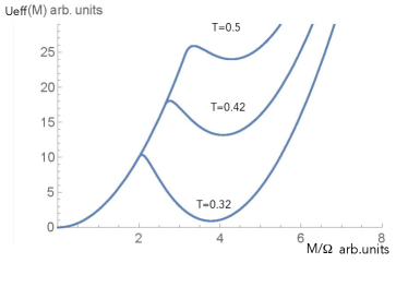
Figure 1: The plots of $U_{eff}(M)$ at different normalised temperatures $T/T^{*}$ manifesting characteristic Q-ball local energy minimum at finite amplitude due to condensation of local/Cooper pairs inside Q-balls, obtained from Equations (14) and (15), see text.

III Summary of Theoretical Predictions for Q-Balls

Summarising, Equation (1) was used to describe effective theory of the Fourier components of the leading Q-ball (i.e., short-range) SDW/CDW fluctuations. Explicit expression for $U_{f}(|M(\tau,{\bf{r}})|)$ was derived and investigated in detail previously Mukhin(2022) ; Mukhin(2022_1) by integrating out Cooper/local-pairs fluctuations in the ‘nested’ Hubbard model with charge-/spin-fermion interactions. As a result, Q-ball self-consistency Equation (12) was solved and investigated, and it was established that Euclidean Q-balls describe stable semiclassical short-range charge/spin-ordering fluctuations of finite energy that appear at finite temperatures below some temperature T^∗, found to be $T^{*}\approx\mu_{0}/2\pi$ Mukhin(2022) ; Mukhin(2022_1) . Next, it was also found that transition into pseudogap phase at the temperature T^∗ is of 1st order with respect to the amplitude $M$ of the Q-ball SDW/CDW fluctuation and of 2nd order with respect to the superconducting gap $g_{0}$. In particular, the following temperature dependences of these characteristics of the Q-balls were derived from Equations (12), (13), and (15) in the vicinity of the transition temperature T^∗ into pseudogap phase Mukhin(2022_1) for the CDW/SDW amplitude:

$$M=\Omega\left(1+\left(\dfrac{T^{*}-T}{\mu_{0}}\right)^{\frac{2}{5}}\left(\dfrac{15\mu^{2}_{0}}{4\sqrt{2}g\nu}\right)^{\frac{2}{5}}\right),\quad T^{*}=\dfrac{\mu_{0}}{2\pi}\,,$$ (16)

and for the pseudogap $g_{0}$:

$$g_{0}^{2}=\left({T}^{*}-T\right)^{\frac{2}{5}}{\Omega}^{2}\left(\dfrac{15\mu_{0}}{g\nu}\right)^{\frac{2}{5}},$$ (17)

which follows after substitution of Equation (16) into Equation (13). These dependences are plotted in Figure 5b in Mukhin(2022_1) .

III.1 Temperature dependences of Q-ball parameters close to $T^{*}$

Strikingly, but it follows from Equation (17), that micro X-ray diffraction data also allow to infer an emergence of superconducting condensates inside the Q-balls below T^∗. The reason is in the inflation of the volume, which is necessary to stabilise the superconducting condensate at vanishing density. Indeed, this is the most straightforward to infer from linearised Ginzburg–Landau (GL) equation aaa for the superconducting order parameter $\Psi$ of a Q-ball of radius $R$ in the spherical coordinates:

$$-\dfrac{\hbar^{2}}{4m}\ddot{\chi}={bg_{0}^{2}}\chi\;;\quad\Psi(\rho)=\dfrac{C\chi(\rho)}{\rho}\;;\quad\Psi(R)=0,$$ (18)

where $g_{0}^{2}$ from Equation (13) substitutes GL parameter $a=\alpha\cdot(T_{c}-T)/T_{c}$ modulo dimensionful constant $b$ of GL free energy functional aaa . Then, it follows directly from solution of Equation (18):

$${\chi}\propto\sin(k_{n}\rho)\;;\quad Rk_{n}=\pi n,\;;\quad n=1,2,...,$$ (19)

that Equation (18) would possess solution (19) with the eigenvalue ${bg_{0}^{2}}$ only if the Q-ball radius is greater than $R_{min}$:

$$\dfrac{\hbar^{2}}{4m}\left(\dfrac{\pi}{R_{min}}\right)^{2}={bg_{0}^{2}}.$$ (20)

Hence, due to conservation condition Equation (8), charge Q should obey the following condition:

$${Q}\geq Q_{min}\equiv{\Omega M^{2}}(R_{m})^{3}={\Omega M^{2}}\dfrac{(\pi\hbar)^{3}}{g_{0}^{3}(4mb)^{3/2}}\;.$$ (21)

This would have an immediate influence on the temperature dependence of the most probable value of charge Q. The letter value could be evaluated using expression for the Q-ball energy Equation (11): $E_{Q}={2Q\Omega}/{g}$ obtained in Mukhin(2022) . Then, Boltzmann distribution of energies of the Q-balls ‘gas’ indicates that the most numerous, i.e., the most probable to occur, Q-balls are those with the smallest possible charge Q, and their respective population (overage) number $\bar{n}_{Q}$ in unit volume of the sample is:

$$\bar{n}_{Q}\propto\dfrac{1}{V}G_{Q}\exp{\left\{-\dfrac{E_{Q}}{k_{B}T}\right\}}=G_{Q}\exp{\left\{-\dfrac{2Q\Omega}{gk_{B}T}\right\}}\;,G_{Q}=\dfrac{V}{V_{Q}},$$ (22)

where $G_{Q}$ counts the number of possible Q-ball ‘positions’ in the sample of volume $V$, $V_{Q}$ being Q-ball volume, and $\Omega/k_{B}T=2\pi$. Hence, Equation (22) indicates that the Boltzmann’s exponent is greater for smaller $Q$. On the other hand, due to accommodated superconducting condensates inside the Q-balls, their Noether charge Q is limited from below by Q_min, as demands Equation (21). Substituting into Equations (20) and (21) temperature dependences of $M$ and $g_{0}$ from Equations (16) and (17), one finds:

$$R_{min}=\dfrac{1}{\Omega(T^{*}-T)^{1/5}}\dfrac{\pi\hbar}{\sqrt{4mb}}\left(\dfrac{g\nu}{15\mu_{0}}\right)^{1/5}\,;$$ (23)

$$M^{2}=\Omega^{2}\left(1+\left(\dfrac{T^{*}-T}{\mu_{0}}\right)^{\frac{2}{5}}\left(\dfrac{15\mu^{2}_{0}}{4\sqrt{2}g\nu}\right)^{\frac{2}{5}}\right)^{2}\,;$$ (24)

$$Q_{min}=\left(1+\left(\dfrac{T^{*}-T}{\mu_{0}}\right)^{\frac{2}{5}}\left(\dfrac{15\mu^{2}_{0}}{4\sqrt{2}g\nu}\right)^{\frac{2}{5}}\right)^{2}\dfrac{(\pi\hbar)^{3}}{(4mb)^{3/2}(T^{*}-T)^{3/5}}\left(\dfrac{g\nu}{15\mu_{0}}\right)^{3/5}$$ (25)

An immediate measurable consequence of the Q-ball charge conservation in the form of Eq. (8) would be inverse correlation between Q-ball volume $V_{Q}=4\pi R_{Q}^{3}/3$ and CDW/SDW amplitude squared $M^{2}$ at fixed temperature $T=\Omega/2\pi$. This anticorrelation might be extracted e.g. from experimental X-ray scattering data campi22 in the form of dependence of the amplitude $A\sim M^{2}$ of X-ray scattering peak on its width in momentum space $\Delta k\sim 1/R_{Q}\sim V_{Q}^{-1/3}$ in the pseudogap phase of high-T_c cupratesMukhin(2022) . In order to make a precise prediction one has to derive X-ray scattering cross-section by Q-balls. Taking into account exponential dependence of the Boltzmann distribution of the energies of the Q-balls on their ‘Noether charge’ Q and their respective population (overage) number $\bar{n}_{Q}$ in Eq. (22), one may fix $Q=Q_{min}$ close enough to the transition temperature $T^{*}$ in the farther derivations of the X-ray scattering cross-section by the Q-balls presented below.

IV Bragg’s law for X-ray scattering by Q-balls

IV.1 Photon Green’s function in Q-balls gas

Using phonon-like ansatz for the photon Green’s function $D_{0}(\tau,{\bf{r}})$ in ideal crystal and then introducing photon scattering by the Q-ball scalar field $M(\tau,{\bf{r}})$ defined in Eqs. (2), (7), one finds the following equation after averaging over positions of the Q-ball centres in space and over zero-origin $\tau_{0}$ of Matsubara time, compare with random space impurity scattering technique agd :

$$D({r}-{r}^{\prime})=D_{0}({r}-{r}^{\prime})+$$

$$+\gamma^{2}\displaystyle\sum_{Q}\bar{n}_{Q}\int d^{4}r_{1}d^{4}r_{2}D_{0}({r}-{r}_{1})D_{M}^{Q}({r}_{1}-{r}_{2})D({r}_{1}-{r}_{2})D({r}_{2}-{r}^{\prime})\,$$ (26)

$$r\equiv\{\tau,{\bf{r}}\},\;\int d^{4}r\equiv\int_{0}^{\beta}d\tau\int d^{3}{\bf{r}}\,,$$

where $\bar{n}_{Q}$ is given in Eq. (22), interaction constant $\gamma$ sets the scale of the scattering amplitude of X-ray photon on the Q-ball field, and Boltzmann distribution of the Q-balls energies $E_{Q}$, given in Eq. (11), regulates via $\bar{n}_{Q}$ a density of Q-balls gas. The most probable to occur Q-balls are those with the smallest possible charge $Q=Q_{min}$, and $G_{Q}$ counts the number of possible ‘positions’ for a Q-ball in the sample of volume $V$, $V_{Q}$ being Q-ball’s volume, and $\Omega/k_{B}T=2\pi$. A Q-ball field correlator $D_{M}^{Q}(\tau,{\bf{r}})$ is obtained by using Eqs. (2), (7) and averaging over origin $\tau_{0}$ of Matsubara time:

$$D_{M}^{Q}(\tau,{\bf{r}})=2M^{2}\exp\{-{r}{\kappa}\}\cos{({\bf{Q}}\cdot{\bf{r}}-\Omega\tau)};\quad\kappa=\dfrac{1}{R_{Q}},\;R_{Q}=\left(3V_{Q}/4\pi\right)^{1/3}.$$ (27)

for a Q-ball of radius $R_{Q}$. The upper index $Q$ in $D_{M}^{Q}$ signifies dependence of parameter $\kappa$ on the charge $Q$ in accord with Eqs. (8), (10). Equation (26) in diagrammatic form is presented in Fig. 2.

Figure 2: The Dyson equation for X-ray scattering by Q-balls of CDW/SDW bosonic field : the dashed line is CDW/SDW Q-ball bosonic Euclidean field correlator $D_{M}^{Q}$ averaged over coordinates of Q-ball’s centres in a crystal and Matsubara time zero-origin $\tau_{0}$. Heavy and thin lines are photon’s temperature Green’s functions $D({r}-{r}^{\prime})$ and $D_{0}({r}-{r}^{\prime})$ respectively. Crosses are vertices of X-ray photon-Q-ball field interaction $\gamma$.

In order to pass to momentum representation in Eq. (26) one has to calculate the Fourier transform of the Q-ball field correlator $D_{M}^{Q}(\tau,{\bf{r}})$ defined in Eq. (27):

$$D_{M}^{Q}(\omega,{\bf{q}})={2M^{2}}{\int^{1/T}_{0}}d\tau\int d^{3}{\bf{r}}\cos{({\bf{Q}}\cdot{\bf{r}}-\Omega\tau)}\exp\{-r\kappa\ -i({\bf{q}}\cdot{\bf{r}}-i\omega\tau)\}=$$

$$=\dfrac{8\pi M^{2}\kappa}{T}\left[\dfrac{\delta_{\omega,\Omega}}{(({\bf{Q}}-{\bf{q}})^{2}+\kappa^{2})^{2}}+\dfrac{\delta_{\omega,-\Omega}}{(({\bf{Q}}+{\bf{q}})^{2}+\kappa^{2})^{2}}\right]$$ (28)

where $\delta_{i,j}$ is Kronecker delta. Then, Eq.(26) takes the following form in momentum representation:

$$D^{-1}(\omega,{\bf{p}})={D_{0}}^{-1}(\omega,{\bf{p}})-\gamma^{2}T\displaystyle V\sum_{\omega^{\prime},Q}\bar{n}_{Q}\int d^{3}{\bf{q}}D_{M}^{Q}(\omega^{\prime},{\bf{q}})D(\omega-\omega^{\prime},{\bf{p}}-{\bf{q}})\,;$$ (29)

$${D_{0}}^{-1}(\omega,{\bf{p}})=-\dfrac{\omega^{2}+c^{2}p^{2}}{c^{2}p^{2}}\,,\;\omega=2\pi nT\,;n=\pm 1,\pm 2,...\,.$$ (30)

Here $c$ is light (X-ray radiation) velocity and linear dispersion $\omega_{0}(p)=cp$ is assumed for simplicity. Hence, after tedious, but straightforward calculation one finds photon’s self-energy to the second order in coupling strength $\gamma$ :

$$D^{-1}(\omega,{\bf{p}})={D_{0}}^{-1}(\omega,{\bf{p}})+16\pi^{2}\gamma_{Q}^{2}M^{2}I_{2}(\omega)\,;\quad I_{2}(\omega)=I_{+}+I_{-}\,;$$ (31)

$$I_{+}=\dfrac{\kappa\dfrac{|\omega-\Omega|^{3}}{c^{3}}+\frac{1}{4}\left[\left(\dfrac{\omega-\Omega}{c}\right)^{2}(\Delta^{2}-3\kappa^{2})+(\Delta^{2}+\kappa^{2})^{2}\right]}{\left(\Delta^{2}+\kappa^{2}-\left(\dfrac{\omega-\Omega}{c}\right)^{2}\right)^{2}+4\left(\dfrac{\omega-\Omega}{c}\right)^{2}\Delta^{2}}\,;\quad\Delta\equiv|{\bf{Q}}-{\bf{p}}|\,;$$ (32)

$$I_{-}=I_{+}(-\Omega,-{\bf{Q}}),$$ (33)

$$\gamma_{Q}^{2}\equiv V\bar{n}_{Q}\gamma^{2}\propto\gamma^{2}VV_{Q_{min}}^{-1}\exp{\left\{-\dfrac{2Q_{min}\Omega}{gk_{B}T}\right\}},$$ (34)

where summation over Q-ball charge $Q$ in Eq. (29) is approximately substituted with the number of Q-balls of minimal charge $Q_{min}$ calculated above in Eqs. (21), (25). Next, one has to continue analytically the Green’s function $D$ in Eq. (31) from imaginary axis points $i\omega=2\pi nT$ to real axis $i\omega\rightarrow z$, considering for definiteness e.g. $\Omega=2\pi T>0$, in accord with Eq. (2). Then expressions for the integrals $I_{\pm}$ in Eq. (33) take the form:

$$D^{-1}(z,{\bf{p}})=\dfrac{z^{2}-c^{2}p^{2}}{c^{2}p^{2}}+16\pi^{2}\gamma_{Q}^{2}M^{2}(I_{+}(z)+I_{-}(z))\,;$$ (35)

$$I_{\pm}(z)=\displaystyle\dfrac{i\kappa\dfrac{(i\Omega\mp z)^{3}}{c^{3}}-\frac{1}{4}\left[\left(\dfrac{z\mp i\Omega}{c}\right)^{2}(\Delta_{\pm}^{2}-3\kappa^{2})-(\Delta_{\pm}^{2}+\kappa^{2})^{2}\right]}{\left[\kappa^{2}+\left(\Delta_{\pm}-\left(\dfrac{z\mp i\Omega}{c}\right)\right)^{2}\right]\left[\kappa^{2}+\left(\Delta_{\pm}+\left(\dfrac{z\mp i\Omega}{c}\right)\right)^{2}\right]}\;,$$ (36)

$$\Delta_{\pm}=|{\bf{Q}}\mp{\bf{p}}|.$$ (37)

It is easy to check, using Eq. (27) for the Q-ball field correlator, that contributions due to terms $I_{\pm}$ in Eq. (36), (37) are space-time (PT) symmetric, see also Fig. (3a,b). First, consider for definiteness pole of $D(z,{\bf{p}})$ when contribution due to $I_{+}(z)$ dominates and $I_{-}(z)$ is negligible. Then, remarkably, the term with $I_{+}(z)$ leads to a famous Bragg’s reflection law Bragg in the scattering configuration in Fig. (3a) with finite life-time, that gives X-ray scattering intensity, see Eq. (39) below.

Figure 3: a. Bragg’s reflection of incident X-ray (wave vector ${\bf{p}}$) by the Q-ball with wave-vector ${\bf{Q}}$ described with the term $I_{+}$ in Eqs. (35) - (39), see text. b. The space-time (PT) symmetric scattering event described by term with $I_{-}$ in Eq. (35).

Assume that relation between frequency and momentum of the photon is weakly disturbed by scattering, i.e. $z^{2}\approx c^{2}p^{2}$ according to Eq. (35). Then, momentum of the incident photon minimises denominator of $I_{+}(z)$ when $|{\bf{Q}}-{\bf{p}}|-|{\bf{p}}|=0$. The latter relation, according to Fig. (3) and notations therein, turns into Bragg’s rule for X-rays reflection by the Q-ball:

$${2}\dfrac{2\pi}{Q}\sin{\Theta}\equiv{2}d\sin{\Theta}={\lambda_{p}}\equiv\dfrac{2\pi}{p},$$ (38)

where $d=2\pi/Q$ is period of CDW/SDW, see Fig. (3), and $\lambda_{p}$ is wave length of the X-ray photon with wave vector $p$ (Plank’s constant $\hbar=1$). Expanding $I_{+}$ in Eq. (36) in the vicinity of wave vector ${\bf{p}}$ obeying the Bragg’s relation $|{\bf{Q}}-{\bf{p}}|-|{\bf{p}}|=0$ in (38) one finds:

$${D_{R}}^{-1}(\omega,{\bf{p}})=\dfrac{\omega^{2}-c^{2}p^{2}}{c^{2}p^{2}}+\dfrac{2\pi^{2}\gamma_{Q}^{2}M^{2}\left[|{\bf{Q}}-{\bf{p}}|\left(|{\bf{Q}}-{\bf{p}}|-\dfrac{\omega}{c}\right)+i\dfrac{\Omega\omega}{c^{2}}\right]}{\kappa^{2}+\left(|{\bf{Q}}-{\bf{p}}|-\dfrac{\omega}{c}\right)^{2}},$$ (39)

where $\Gamma$ is scattering intensity of X-ray photon with momentum ${\bf{p}}$ by a single Q-ball with wave-vector ${\bf{Q}}$, and real frequency variable $z$ is substituted with a common notation $\omega$ giving X-ray energy $\hbar\omega$. The overall line shape of the X-ray scattering peak, characterised by $-\frac{1}{\pi}Im{D_{R}}(z,{\bf{p}})$ then reads:

$$-\dfrac{1}{\pi}Im{D_{R}}(\omega,{\bf{p}})=\dfrac{\Gamma(\omega,{\bf{p}})}{\left[\dfrac{\left(\dfrac{\omega}{c}\right)^{2}-p^{2}}{p^{2}}+\dfrac{2\pi^{2}\gamma_{Q}^{2}M^{2}p|{\bf{Q}}-{\bf{p}}|\left(|{\bf{Q}}-{\bf{p}}|-\dfrac{\omega}{c}\right)}{\kappa^{2}+\left(|{\bf{Q}}-{\bf{p}}|-\dfrac{\omega}{c}\right)^{2}}\right]^{2}+\Gamma(\omega,{\bf{p}})^{2}}$$ (40)

$$\Gamma(\omega,{\bf{p}})=\dfrac{2\pi^{2}\gamma_{Q}^{2}M^{2}{\Omega\omega}}{{c^{2}}\left(\kappa^{2}+\left(|{\bf{Q}}-{\bf{p}}|-\dfrac{\omega}{c}\right)^{2}\right)},$$ (41)

$$\kappa^{2}\geq\left(|{\bf{Q}}-{\bf{p}}|-p\right)^{2}\,,$$ (42)

IV.2 X-ray diffraction pattern in Q-balls gas

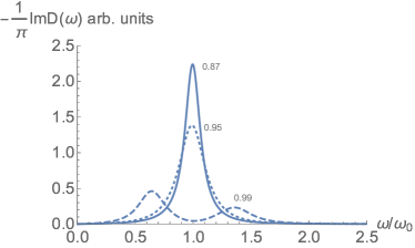
Figure 4: Q-ball scattered X-ray Green’s function $-\dfrac{1}{\pi}Im{D_{R}}(\omega,{\bf{p}})$ in Eq. (40) at different temperatures indicated by $T/T^{*}$ ratios as function of wave-vector $p$ expressed via frequency $cp=\omega$ in units of incident X-ray frequency $\omega_{0}$, with dimensionless scattering amplitude $g=0.115$ defined as: $2\pi^{2}\gamma_{Q}^{2}M^{2}\Omega/T^{*}\equiv g(T/T^{*})^{3}$.

The above expression for the Green’s function of the X-ray photon scattered by Q-balls is remarkable: besides information on the X-ray scattering intensity it contains the famous Bragg’s reflection law Bragg , when the Q-ball radius $R$ is big enough with respect to photon wave length $\lambda\sim 1/p$, i.e. $1/R\sim\kappa\ll p$ in Eq. (38). The X-ray scattering intensity is characterized by imaginary part of the Green’s function $-\dfrac{1}{\pi}Im{D_{R}}(\omega,{\bf{p}})$ in Eq. (40) which provides the density of states of the scattered X-rays with energy $\hbar\omega$, see Fig. 4.

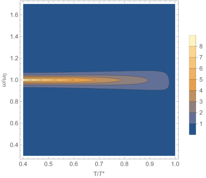
(a) a)

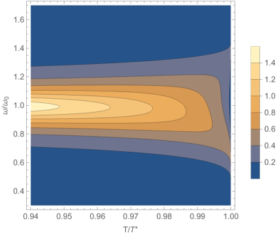
(b) b)

Figure 5: Q-ball scattered X-ray spectral line given by false colour intensity plots a) of the Green’s function $-\dfrac{1}{\pi}Im{D_{R}}(\omega,{\bf{p}})$ in Eq. (40) at different temperatures indicated by $T/T^{*}$ ratios as function of frequency/wave-vector $p$ expressed as dimensionless frequency $\omega=cp$ in units of incident X-ray frequency $\omega_{0}$, with dimensionless scattering amplitude $g=0.115$ defined as in Fig. 4; b) is the same as a) but with higher resolution in temperature $T\approx T^{*}$. The picture is in good correspondence with experimental plot in Fig. 1 of the recently published X-ray diffraction data campi22 for the short-range dynamic CDW satellite peak intensity that appeared below $T^{*}$ temperature.

The splitting of the peak into two at temperatures close to $T^{*}$ follows directly from Eq. (40) and will be evaluated below in analytic form. The scattered X-rays line shape is also possible to represent in a form of the false color plots in Fig. 5 as generated from Eq. (40), with the splitting of the peaks in Fig. 4 at temperatures very close to $T^{*}$ resulted in Fig. 5b. The figure Fig. 5a dramatically resembles experimental plots published recently campi22 . Next, there are two opposite limits that can be used to derive analytically treatable consequences from the general Eq. (40). Namely, consider first the limit $\pi\gamma Mp\ll\kappa\approx R_{min}^{-1}$, where $R_{min}$ is the most probable Q-ball size close to $T^{*}$ temperature given by Eq. (23). Then, Eq. (40) is reduced to a single Lorentzian:

$$-\dfrac{1}{\pi}Im{D_{R}}(\omega,{\bf{p}})\approx\dfrac{\tilde{\Gamma}(\omega,{\bf{p}})}{\dfrac{4}{p^{2}}\left(\dfrac{\omega}{c}-p\right)^{2}+\tilde{\Gamma}^{2}(\omega,{\bf{p}})},$$ (43)

$$\tilde{\Gamma}(\omega,{\bf{p}})=\dfrac{2\pi^{2}\gamma_{Q}^{2}M^{2}{\Omega p}}{{c}\kappa^{2}},$$ (44)

$$-\dfrac{1}{\pi}Im{D_{R}}(\omega,{\bf{p}})_{max}=\pi^{-1}\tilde{\Gamma}^{-1}(\omega,{\bf{p}}).$$ (45)

Hence, the amplitude of the Lorentzian peak in Eq. (45) equals $\pi^{-1}\tilde{\Gamma}^{-1}(\omega,{\bf{p}})$. Substituting temperature dependences of all the parameters entering the Lorentzian peak amplitude in Eq. (45) from Eqs. (23), (24) one finds the following theoretical dependences plotted in Fig.6 of different characteristics of X-ray scattering.

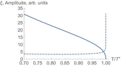
(a) a)

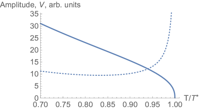
(b) b)

Figure 6: a) Theoretical temperature dependence of the SDW/CDW single Q-ball scattered X-rays line peak amplitude and inverse of the peak width $\xi$: $-\dfrac{1}{\pi}Im{D_{R}}(\omega,{\bf{p}})_{max}$ (solid line), $\xi=R_{min}$ (dashed line), as functions of reduced temperature expressed in units of ${T/T^{*}}$; b) solid line is the same as in a), dotted line is Q-ball volume $V_{Q}\propto R_{min}^{3}$ as function of reduced temperature ${T/T^{*}}$. The pictures are in good correspondence with experimental plots in Fig. 2 of the recently published X-ray diffraction data campi22 for the short-range dynamic CDW X-rays scattering satellite peak intensity that appeared below $T^{*}$ temperature.

These plots are in good qualitative correspondence with the experimental data of the X-ray scattering in high-$T_{c}$ cuprates HgBa₂CuO_4+y campi22 .

V Q-ball mechanism of the $T$-linear temperature dependence of electrical resistivity in strange metal phase

The above derivation of the X-ray diffraction by Q-balls could be now adjusted to show a cause of linear temperature dependence of electrical resistivity of the high-T_c superconductor in the Q-ball fluctuations phase described in this paper.

Figure 7: The Dyson equation for a fermion scattering by Q-balls of CDW/SDW bosonic field : the dashed line is CDW/SDW Q-ball bosonic Euclidean field correlator $D_{M}^{Q}$ averaged over coordinates of Q-ball’s centres in a crystal and Matsubara time zero-origin $\tau_{0}$. Heavy and thin lines are fermionic temperature Green’s functions $G({r}-{r}^{\prime})$ and $G_{0}({r}-{r}^{\prime})$ respectively. Dots are vertices of fermion- Q-ball field $M$ interaction Eq. (46).

Consider now Fig. 7, where now, contrary to Fig. 2, the heavy and thin lines are fermionic temperature Green’s functions $G({r}-{r}^{\prime})$ and $G_{0}({r}-{r}^{\prime})$ respectively, that depend on the differences of the $D+1$ coordinates after averaging over position of a Q-ball in space and Matsubara time origin $\tau_{0}$. Dots are vertices of fermion- Q-ball field $M$ interaction introduced in Mukhin(2022) ; Mukhin(2022_1) via the expression:

$${S}_{f}=\int_{0}^{\beta}\int_{V}d\tau d^{D}{\bf{r}}\sum_{{\bf{q}},\sigma}\left[c^{+}_{{\bf{q}}\sigma}(\partial_{\tau}+\varepsilon_{q})c_{{\bf{q}},\sigma}+\left(c^{+}_{{\bf{q+Q}_{DW}},\sigma}M(\tau,{\bf{r}})\sigma c_{{\bf{q}},\sigma}+H.c.\right)\right]\,.$$ (46)

First, some rough evaluation is in order. Consider fermionic momentum uncertainty $\Delta p$ due to finite radius $R_{Q}$ of a Q-ball fluctuation and related uncertainty $\varepsilon_{Q}$ of fermionic excitation energy $\varepsilon$ in the vicinity of Fermi chemical potential:

$$\Delta p\sim\dfrac{\hbar}{R_{Q}};$$ (47)

$$\Delta\varepsilon(p)\equiv\varepsilon_{Q}\sim v_{F}\Delta p\sim v_{F}\dfrac{\hbar}{R_{Q}};$$ (48)

$$\Delta t\Delta\varepsilon(p)\sim\tau_{Q}\Delta\varepsilon(p)\geq\hbar\Rightarrow\dfrac{1}{\tau_{Q}}\sim v_{F}\dfrac{1}{R_{Q}}\,,$$ (49)

where $1/\tau_{Q}$ is fermionic quasiparticle decay rate due to Q-ball fluctuation. Now, using expression for the Q-ball conserved ‘Noether charge’ Q Eq. 8, and temperature dependences for the M-field amplitude in Eq. (16) giving $M\propto T$ well below T^∗ temperature, one finds T-linear dependence of $1/\tau_{Q}$:

$$\dfrac{1}{\tau_{Q}}\sim v_{F}\dfrac{\hbar}{R_{Q}}\sim\left(\dfrac{\Omega M^{2}4\pi}{3Q}\right)^{1/3}\propto\dfrac{T}{{N_{Q}}^{1/3}}\,,$$ (50)

where $N_{Q}=Q/g$ is temperature independent number of condensed charge/spin excitations forming a Q-ball. The temperature independence of $N_{Q}$ follows from the Boltzmann distribution $P(Q)$ of the ”charges” Q via Q-balls energies $E_{Q}$, given in Eq. (11), that prove to be linear temperature dependent:

$$P(Q)\sim\exp\left\{-\dfrac{E_{Q}}{k_{B}T}\right\}\sim\exp\left\{-\dfrac{2Q\Omega}{gk_{B}T}\right\}\equiv\exp\left\{-\dfrac{4\pi Q}{g}\right\},$$ (51)

where definition of bosonic Matsubara frequency $\Omega=2\pi Tn$, $n=1$ was used in accord with Eq. (2). Hence, using $1/\tau_{Q}$ in the Drude like kinetic equation for the fermionic quasiparticle momentum in external electric field one finds T-linear electrical resistivity in the Q-ball fluctuations phase, in qualitative accord with high-T_c cuprates behavior in the strange metal phase Zaanen . Next, a more thorough derivation follows from the Dyson equation in Fig. 7 for the fermionic Green’s function $G$ with M-field bosonic Green’s function ${D^{Q}}_{M}$ given in Eq. (28):

$$G(\omega,p)=\dfrac{1}{i\omega-\xi-\bar{G}};\quad\xi=v_{F}(|{p}|-p_{F})$$ (52)

$$\bar{G}(\omega,p)=\sum_{Q}n_{Q}M^{2}\dfrac{8\pi\kappa\hbar}{(2\pi)^{3}}\int d^{3}\vec{p}_{1}\left\{\dfrac{G(\vec{p}_{1},\omega-\Omega)}{(\vec{p}-\vec{p}_{1}-\vec{Q})^{2}+\kappa^{2}}+\dfrac{G(\vec{p}_{1},\omega+\Omega)}{(\vec{p}-\vec{p}_{1}+\vec{Q})^{2}+\kappa^{2}}\right\}=$$

$$=\dfrac{4}{\pi}\sum_{Q}n_{Q}M^{2}\varepsilon_{Q}\left(I_{+}+I_{-}\right)\,;\quad I_{\pm}=\int^{\infty}_{-\infty}\dfrac{d\xi}{\left[i(\omega\mp\Omega)-\xi-\bar{G}_{\pm}\right]\left[{\varepsilon_{Q}}^{2}+(\xi-\xi_{\pm})^{2}\right]};$$ (53)

$$\xi_{\pm}=v_{F}(|\vec{p}\mp\vec{Q}|-p_{F});\quad\bar{G}_{\pm}=\bar{G}(\omega,|\vec{p}\mp\vec{Q}|);\quad n_{Q}\propto\exp\left\{-\dfrac{4\pi Q}{g}\right\},$$ (54)

that after analytic continuation to the real axis of $\omega$ gives retarded Green’s function:

$$G^{R}(\omega,p)=\dfrac{1}{i\omega-\xi-\bar{G}^{R}};$$ (55)

$$\bar{G}^{R}(\omega,p)={4}\sum_{Q}n_{Q}M^{2}\varepsilon_{Q}\left\{\dfrac{1}{\omega+i\varepsilon_{Q}-\xi_{+}-{\bar{G}^{R}}_{+}}+\dfrac{1}{\omega+i\varepsilon_{Q}-\xi_{-}-{\bar{G}^{R}}_{-}}\right\}\,$$ (56)

$${\bar{G}^{R}}_{\pm}=\bar{G}^{R}(\omega,|\vec{p}\mp\vec{Q}|).$$ (57)

The latter expression for $G^{R}$ finally leads to a scattering crossection renormalised expression for the quasi-particle life-time $\tau_{Q}$:

$$\dfrac{1}{\tau_{Q}}\approx\dfrac{8\sum_{Q}n_{Q}M^{2}}{\varepsilon_{Q}}\propto T\,,$$ (58)

where the last T-linear estimate for $1/\tau_{Q}$ again follows from the mentioned above relations:$M\sim T$, $\varepsilon_{Q}\sim T$ and Eq. (54) for $n_{Q}$.

VI Conclusions

To summarise, one concludes, that presented above theoretical results and their favourable comparison with experiment campi22 ; campi indicate that X-ray diffraction makes ”visible” the gas of Q-balls with Cooper pairs condensates below T*, and hence opens avenue for direct investigation of the thermodynamic quantum time crystals of CDW/SDW densities. In a particular picture related with high-T_c scenario the vanishing density of superconducting condensates at T* leads to inflation of Q-balls sizes, that self-consistently suppresses X-ray Bragg’s peak intensity close to Q-ball phase transition temperature. Linear temperature dependence of electrical resistivity in the Q-ball phase due to scattering of electrons on the condensed charge/spin fluctuations inside Q-balls is also demonstrated. The T-linear dependence of electrical resistivity arises due to inverse temperature dependence of the Q-ball radius as function of temperature in the strange metal phase.

VII ACKNOWLEDGMENTS

The author is grateful to prof. Antonio Bianconi for making available the experimental data on micro X-ray diffraction in high-T_c cuprates prior to publication and to prof. Carlo Beenakker and his group for stimulating discussions of the work. This research was in part supported by Grant No. K2-2022-025 in the framework of the Increase Competitiveness Program of NUST MISIS.

References

- (1) Mukhin, S.I. Euclidean Q-Balls of Fluctuating SDW/CDW in the ’Nested’ Hubbard Model of High-Tc Superconductors as the Origin of Pseudogap and Superconducting Behaviors. Condens. Matter 2022, 7, 31. https://doi.org/10.3390/condmat7020031
- (2) Mukhin, S.I. Euclidean Q-balls of electronic spin/charge densities confining superconducting condensates as the origin of pseudogap and high-Tc superconducting behaviours. Ann. Phys. 2022, 447, 169000. https://doi.org/10.1016/j.aop.2022.169000.
- (3) Mukhin, S.I. Possible Manifestation of Q-Ball Mechanism of High-Tc Superconductivity in X-ray Diffraction. Condens. Matter,8, 16 (2023), https://doi.org/10.3390/condmat8010016.
- (4) Campi, G.; Barba, L.; Zhigadlo, N.D.; Ivanov, A.A.; Menushenkov, A.P.; Bianconi, A. Q-Balls in the pseudogap phase of Superconducting HgBa2CuO4+y. Condens. Matter 2023, 8, 15. https://doi.org/10.3390/condmat8010015.
- (5) Campi, G.; Bianconi, A.; Poccia, N.; Bianconi, G.; Barba, L.; Arrighetti, G.; Innocenti, D.; Karpinski, J.; Zhigadlo, N.D.; Kazakov, S.M.; et al. Inhomogeneity of charge-density-wave order and quenched disorder in a high-Tc superconductor. Nature 2015, 525, 359–362.
- (6) Li, L.; Wang, Y.; Komiya, S.; Ono, S.; Ando, Y.; Gu, G.D.; Ong, N.P. Diamagnetism and Cooper pairing above Tc in cuprates. Phys. Rev. B 2010, 81, 054510.
- (7) Uemura, Y.J.; Luke, G.M.; Sternlieb, B.J.; Brewer, J.H.; Carolan, J.F.; Hardy, W.; Yu, X.H. Universal correlations between Tc and ns/m* in high-Tc cuprate superconductors. Phys. Rev. Lett. 1989, 62, 2317–2320.
- (8) Bednorz, J.G.; Müller, K.A. Possible highTc superconductivity in the Ba-La-Cu-O system. Z. Phys. B 1986, 64, 189.
- (9) Gao, L.; Xue, Y.Y.; Chen, F.; Xiong, Q.; Meng, R.L.; Ramirez, D.; Chu, C.W.; Eggert, J.H.; Mao, H.K. Superconductivity up to 164 K in HgBa2Cam-1CumO2m+2+δ (m=1, 2, and 3) under quasihydrostatic pressures. Phys. Rev. B 1994, 50, 4260.
- (10) Nagamatsu, J.; Nakagawa, N.; Muranaka, T.; Zenitani, Y.; Akimitsu, J. Superconductivity at 39 K in magnesium diboride. Nature 2001, 410, 63.
- (11) Kamihara, Y.; Hiramatsu, H.; Hirano, M.; Kawamura, R.; Yanagi, H.; Kamiya, T.; Hosono, H. Iron-Based Layered Superconductor: LaOFeP. J. Am. Chem. Soc. 2006, 128, 10012. https://doi.org/10.1021/ja063355c .
- (12) Ozawa, T.C.; Kauzlarich, S.M.; Chemistry of layered d-metal pnictide oxides and their potential as candidates for new superconductors. Sci. Technol. Adv. Mater. 2008, 9, 033003.
- (13) Hashimoto, M.; He, R.-H.; Tanaka, K.; Testaud, J.-P.; Meevasana, W.; Moore, R.G.; Lu, D.; Yao, H.; Yoshida, Y.; Eisaki, H.; et al. Particle—Hole symmetry breaking in the pseudogap state of Bi2201. Nat. Phys 2010, 6, 414. https://doi.org/10.1038/nphys1632.
- (14) Davis, J.C.S.; Lee, D.-H. Concepts relating magnetic interactions, intertwined electronic orders, and strongly correlated superconductivity. Proc. Natl. Acad. Sci. USA 2013, 110, 17623. https://doi.org/10.1073/pnas.1316512110.
- (15) Tranquada, J.M.; Gu, G.D.; Hücker, M.; Jie, Q.; Kang, H.-J.; Klingeler, R.; Li, Q.; Tristan, N.; Wen, J.S.; Xu, G.Y.; et al. Evidence for unusual superconducting correlations coexisting with stripe order in La1.875Ba0.125CuO4. Phys. Rev. B 2008, 78, 174529.
- (16) Bardeen, J.; Cooper, L.N.; Schrieffer, J.R. Microscopic Theory of Superconductivity. Phys. Rev. 1957, 106, 162.
- (17) Fradkin, E.; Kivelson, S.A.; Tranquada, J.M. Colloquium: Theory of intertwined orders in high temperature superconductors. Rev. Mod. Phys. 2015, 87, 457.
- (18) Keimer, B.; Kivelson, S.; Norman, M.; Uchida, S.; Zaanen, J. From quantum matter to high-temperature superconductivity in copper oxides. Nature 2015, 518, 179. https://doi.org/10.1038/ nature14165.
- (19) Coleman, S.R. Q-balls. Nuclear Phys. B 1985, 262, 263–283.
- (20) Rosen, G. Particlelike Solutions to Nonlinear Complex Scalar Field Theories with PositiveDefinite Energy Densities. J. Math. Phys. 1968, 9, 996. https://doi.org/10.1063/1.1664693.
- (21) Lee, T.D.; Pang, Y. Nontopological solitons. Phys. Rept. 1992, 221, 251–350.
- (22) Mukhin, S.I. Negative Energy Antiferromagnetic Instantons Forming Cooper-Pairing Glue and Hidden Order in High-Tc Cuprates. Condens. Matter 2018, 3, 39.
- (23) Eliashberg, G.M. Interactions between electrons and lattice vibrations in a superconductor. JETP 1960, 11, 696–702.
- (24) Abanov, A.; Chubukov, A.V.; Schmalian, J., Quantum-critical theory of the spin-fermion model and its application to cuprates: Normal state analysis. Adv. Phys. 2003, 52, 119–218.
- (25) Seibold, G.; Arpaia, R.; Peng, Y.Y.; Fumagalli, R.; Braicovich, L.; Di Castro, C.; Caprara, S. Strange metal behaviour from charge density fluctuations in cuprates. Commun. Phys. 2021, 4, 1–6.
- (26) Bianconi, A.; Missori, M. The instability of a 2D electron gas near the critical density for a Wigner polaron crystal giving the quantum state of cuprate superconductors. Solid State Commun. 1994, 91, 287–293.
- (27) Abrikosov, A.A.; Gor’kov, L.P.; Dzyaloshinski, I.E. Methods of Quantum Field Theory in Statistical Physics; Dover Publications: New York, NY, USA, 1963.
- (28) Derrick, G.H. Comments on nonlinear wave equations as models for elementary particles. J. Math. Phys. 1964, 5, 1252–1254.
- (29) Bragg, W. L. , The diffraction of short electromagnetic waves by a crystal; Proc. Cambridge Philos. Soc. 17, 43?57 (1913).
- (30) Abrikosov, A.A. Fundamentals of the Theory of Metals; Elsevier Science Publishers B.V.: Amsterdam, The Netherlands, 1988; Chapter 17.
- (31) Feodor V. Kusmartsev, Daniele Di Castro, Ginestra Bianconi, Antonio Bianconi, Transformation of strings into an inhomogeneous phase of stripes and itinerant carriers. Phys. Lett. A 2000, 275, 118–123.
- (32) Masella, G.; Angelone, A.; Mezzacapo, F.; Pupillo, G.; Prokof´ev, N.V. Supersolid Stripe Crystal from Finite-Range Interactions on a Lattice. Phys. Rev. Lett. 2019, 123, 045301.
- (33) Innocenti, D.; Ricci, A.; Poccia, N.; Campi, G.; Fratini, M.; Bianconi, A. A Model for Liquid-Striped Liquid Phase Separation in Liquids of Anisotropic Polarons. J. Supercond. Nov. Magn. 2009, 22, 529–533. https://doi.org/10.1007/s10948-009-0474-9.
- (34) Trugenberger, C.A., Magnetic Monopoles, Dyons and Confinement in Quantum Matter. Condens. Matter 2023, 8, 2. https://doi.org/10.3390/condmat8010002.
- (35) Li, H.; Zhou, X.; Parham, S.; Gordon, K.N.; Zhong, R.D.; Schneeloch, J.; Gu, G.D.; Huang, Y.; Berger, H.; Arnold, G.B.; et al. Four-legged starfish-shaped Cooper pairs with ultrashort antinodal length scales in cuprate superconductors. arXiv 2018, arXiv:1809.02194.