How Well Does the Metropolis Algorithm Cope
With Local Optima?

Abstract.

The Metropolis algorithm (MA) is a classic stochastic local search heuristic. It avoids getting stuck in local optima by occasionally accepting inferior solutions. To better and in a rigorous manner understand this ability, we conduct a mathematical runtime analysis of the MA on the CLIFF benchmark. Apart from one local optimum, cliff functions are monotonically increasing towards the global optimum. Consequently, to optimize a cliff function, the MA only once needs to accept an inferior solution. Despite seemingly being an ideal benchmark for the MA to profit from its main working principle, our mathematical runtime analysis shows that this hope does not come true. Even with the optimal temperature (the only parameter of the MA), the MA optimizes most cliff functions less efficiently than simple elitist evolutionary algorithms (EAs), which can only leave the local optimum by generating a superior solution possibly far away. This result suggests that our understanding of why the MA is often very successful in practice is not yet complete. Our work also suggests to equip the MA with global mutation operators, an idea supported by our preliminary experiments.

1. Introduction

A major difficulty faced by many search heuristics is that the heuristic might run into a local optimum and then find it hard to escape from it. A number of mechanisms have been proposed to overcome this difficulty, e. g., restart mechanisms, discarding good solutions (non-elitism), tabu mechanisms, global mutation operators (which can, in principle, generate any solution as offspring), or diversity mechanisms (which prevent a larger population to fully converge into a local optimum). While all these ideas have been successfully used in practice, a rigorous understanding of how these mechanisms work and in which situation to employ which one, is still largely missing.

To shed some light on this important question, we analyze how the Metropolis algorithm (MA) profits from its mechanism to leave local optima. The MA is a simple randomized hillclimber except that it can also accept an inferior solution. This happens with some small probability which depends on the degree of inferiority and the temperature, the only parameter of the MA. Choosing the right temperature is a delicate problem – a too low temperature makes it hard to leave local optima, whereas a too high temperature forbids an effective hillclimbing.

From this description of the MA one might speculate that the MA copes particularly well with local optima that are close (and thus easy to reach) to inferior solutions from which improving paths lead away from the local optimum. The main result of this work is that this is not true. We conduct a rigorous runtime analysis of the MA on the Cliff benchmark, in which every local optimum is a neighbor of a solution from which improving paths lead right to the global optimum. For this classic benchmark, we prove that the MA even with the optimal (instance-specific) temperature is less efficient on most problem instances than a simple elitist mutation-based algorithm called ${(1+1)}$ EA with standard mutation rate. If the ${(1+1)}$ EA uses an optimized mutation rate, then this discrepancy is even more pronounced. Our experimental results support these findings and show that also several other simple heuristics using global mutation clearly outperform the MA on cliff functions. These results have motivated us to conduct preliminary experiments with the MA equipped with a global mutation operator instead of the usual one-bit flips. While not fully conclusive, these experiments generally show a good performance of the MA with global mutation operators on Cliff. We note that this idea, replacing local mutation by global mutation in a local search heuristic was taken up in (Doerr et al., 2023a) and proven to give significant performance gains when the move acceptance hyper-heuristic optimizes the Cliff benchmark.

For reasons of space, in the conference version (Doerr et al., 2023b) we can only sketch the proofs of our mathematical results. The appendix of this preprint contains the missing proofs.

2. Previous Works

The mathematical runtime analysis of randomized search heuristics has produced a decent number of results on how elitist evolutionary algorithm cope with local optima, but much fewer on other algorithms. The majority of results on evolutionary algorithms concern mutation-based algorithms. Results derived from the Jump benchmark suggest that higher mutation rates or a heavy-tailed random mutation rate (Doerr et al., 2017) as well as a stagnation-detection mechanism (Rajabi and Witt, 2022, 2023, 2021; Doerr and Rajabi, 2023) can speed up leaving local optima. Some examples have been given where elitist crossover-based algorithms coped remarkably well with local optima (Jansen and Wegener, 2002; Dang et al., 2018; Rowe and Aishwaryaprajna, 2019; Antipov et al., 2020), but it is not clear to what extent these results generalize (Witt, 2021).

There are a few runtime results on non-elitist evolutionary algorithms, however, they do not give a very conclusive picture. The results of Jägersküpper and Storch (2007); Lehre (2010, 2011); Rowe and Sudholt (2014); Doerr (2022); Hevia Fajardo and Sudholt (2021) show that in many situations, there is essentially no room between a regime with low selection pressure, in which the algorithm cannot optimize any function with unique optimum efficiently, and a regime with high selection pressure, in which the algorithm essentially behaves like its elitist counterpart. Only with a very careful parameter choice, one can profit from non-elitism in a small middle regime. For example, with a population size of order $\Theta(\log n)$, the ${(1,\lambda)}$ EA can optimize the function $\textsc{Cliff}_{\frac{n}{3}-\frac{3}{2},\frac{n}{3}}$ in polynomial time (Hevia Fajardo and Sudholt, 2021). However, the exponential dependence of the runtime on $\lambda$, roughly $6.20^{\lambda}$, implies that this algorithm parameter has to be chosen very carefully. Other examples of successful applications of non-elitism in evolutionary algorithms exist, e.g., Dang et al. (2021). Most of these works do not regard classic benchmarks, but artificial problems designed to demonstrate that a particular behavior can happen, so it is usually difficult to estimate how widespread this behavior really is. The very recent work (Jorritsma et al., 2023) shows moderate advantages of comma selection on randomly disturbed OneMax functions.

Outside the range of well-established search heuristics, Paixão et al. (2017) show that the strong-selection weak-mutation process from biology can optimize some functions faster than elitist evolutionary algorithms. Lissovoi et al. (2023) show that the move-acceptance hyper-heuristic proposed by Lehre and Özcan (2013) can optimize cliff functions in cubic time. However, as recently shown in (Doerr et al., 2023a), it performs significantly worse than most EAs on the Jump benchmark.

For the MA algorithm, the rigorous understanding is less developed than for EAs. The classic result of Sasaki and Hajek (1988) shows that the MA can compute good approximations for the maximum matching problem. An analogous result was shown for the ${(1+1)}$ EA (Giel and Wegener, 2003), demonstrating that this problem can also be solved via elitist methods. Jerrum and Sorkin (1998) showed that the MA can solve certain random instances of the minimum bisection problem in quadratic time.

Jansen and Wegener (2007) conducted a runtime analysis of MA on the classic OneMax benchmark. While it is not surprising that the MA does not profit from its ability to accept inferior solutions on this unimodal benchmark, their result shows that only very small temperatures (namely such that the probability of accepting an inferior solution is at most $O(\log(n)/n)$) lead to polynomial runtimes. As a side result to their study on hyperheuristics, Lissovoi et al. (2023, Theorem 14) show that the MA cannot optimize the multimodal Jump benchmark in sub-exponential time. The same work also contains a runtime analysis on the Cliff problem, which we will discuss in more detail after having introduced this benchmark further below. Wang et al. (2021) show a good performance of the MA on the DLB benchmark (roughly by a factor of $n$ faster than elitist EAs). This problem, first proposed by Lehre and Nguyen (2019) has (many) local optima, however, these are easy to leave since they all have a strictly better solution in Hamming distance two.

Again a number of results exist for artificially designed problems. Among them, Droste et al. (2000) defined a Valley problem that is hard to solve for the MA with any fixed temperature, whereas Simulated Annealing, that is, the MA with a suitable cooling schedule, solves it in polynomial time. Jansen and Wegener (2007) construct an objective function such that the MA with a very small temperature has a polynomial runtime, whereas the ${(1+1)}$ EA needs time $\Omega(n^{\Omega(\log\log n)})$. Oliveto et al. (2018) proposed a problem called Valley, different from the homonymous Valley problem defined by Droste et al. (2000), such that again the MA and the Strong Selection Weak Mutation algorithm have a much better runtime than the ${(1+1)}$ EA. Similar results where obtained for a similar problem called ValleyPath, which contains a chain of several local optima. It should be noted that all these problems were designed to demonstrate a particular difference between two algorithms and are even farther from real-world problems than the classic benchmarks like OneMax, Jump and Cliff. For example, the Valley and ValleyPath problems defined by Oliveto et al. (2018) are essentially a one-dimensional problems that are encoded into the discrete hypercube. For this reason, it is hard to derive general insights from these works beyond the fact that the algorithms regarded can have drastically different performances.

3. Preliminaries

3.1. The Metropolis Algorithm and the ${(1+1)}$ EA

The Metropolis Algorithm (MA) (Metropolis et al., 1953) is a simple single-trajectory search heuristic for pseudo-Boolean optimization. It selects and evaluates a random neighbor of the current solution and accepts it (i) always if it is at least as good as the parent, and (ii) with probability $e^{-\delta/T}$ if its fitness is by $\delta$ worse than the fitness of the current solution. Here $T$, often called temperature, is the single parameter of the MA. See Algorithm 1 for the pseudocode of the MA. To ease our later analyses, we use the parameterization $\alpha=e^{1/T}$, that is, the parameter $\alpha>0$ fixes the probability $\alpha^{-\delta}$ of accepting a solution worse than the parent by $\delta$. The MA and its generalization Simulated Annealing have found numerous successful applications in various areas, see, e.g., van Laarhoven and Aarts (1987); Dowsland and Thompson (2012).

Algorithm 1 The Metropolis algorithm with temperature $T$ for the maximization of $f\colon\{0,1\}^{n}\to\mathbb{R}$. We ususally write $\alpha=e^{1/T}$.

Select $x^{(0)}$ uniformly at random from $\{0,1\}^{n}$.

for $t\leftarrow 0,1,\dots$ do

     Create $y$ by flipping a bit of $x^{(t)}$ chosen uniformly at random.

     if $f(y)\geq f(x^{(t)})$ then

         $x^{(t+1)}\leftarrow y$

     else

         $x^{(t+1)}\leftarrow y$ with probability $e^{(f(y)-f(x^{(t)}))/T}$ and

         $x^{(t+1)}\leftarrow x^{(t)}$ with the remaining probability.      

To understand to what extent the MA profits from its ability to accept inferior solutions, we compare it with a simple elitist stochastic hillclimber, the ${(1+1)}$ EA (Algorithm 2). As the MA, it follows a single search trajectory, however, it never accepts inferior search points. To be able to leave local optima, the ${(1+1)}$ EA does not move to random neighbors of the current solution (that is, generates the new solution by flipping a random bit), but flips each bit of the current solution independently with some probability $p$. A common recommendation for this mutation rate is $p=1/n$, see, e.g., Bäck (1996); Droste et al. (2002); Ochoa (2002); Witt (2013). With this choice, with probability approximately $1/e\approx 0.37$ the new solution is a neighbor of the current search point.

Algorithm 2 The ${(1+1)}$ EA with mutation rate $p$ for the maximization of $f\colon\{0,1\}^{n}\to\mathbb{R}$.

Select $x^{(0)}$ uniformly at random from $\{0,1\}^{n}$.

for $t\leftarrow 0,1,\dots$ do

     Create $y$ by flipping each bit of $x^{(t)}$ independently with probability $p$.

     if $f(y)\geq f(x^{(t)})$ then $x^{(t+1)}\leftarrow y$

     else $x^{(t+1)}\leftarrow x^{(t)}$.      

As runtime $T$ (synonymously, optimization time) of these algorithms, we regard the (random) first point in time $t$ where an optimum has been sampled. We shall mostly be interested in expected runtimes.

3.2. The Cliff and OneMax Functions

The aim of this paper is to study how efficient the MA is at optimizing functions with a local optimum. The two best-studied benchmark functions to model situations with local optima are Jump (Droste et al., 2002) and Cliff (Jägersküpper and Storch, 2007). That the MA has enormous difficulties optimizing Jump was shown by Lissovoi et al. (2023). This result is not too surprising when considering the fitness landscape of Jump. The valley of low fitness separating the local optimum from the global one is deep (it consists of the solutions of lowest fitness) and the fitness gradient is pointing towards the local optimum everywhere in this valley.

For this reason, in this work we analyze the performance of the MA on the Cliff benchmark, where the valley of low fitness is more shallow and the fitness inside the valley is not deceptive, that is, the gradient is pointing towards the optimum. With these properties, Cliff should be a problem where the MA could profit from its ability to occasionally accept an inferior solution. Surprisingly, as our precise analysis for the full spectrum of temperatures will show, this is not true.

Like Jump functions, also Cliff functions were originally defined with only one parameter determining the distance of the local optimum from the global optimum, which also is the width of the valley of fitness lower than the one of the local optimum. Since a series of recent work on the Jump benchmark (Jansen, 2015; Bambury et al., 2021; Rajabi and Witt, 2021; Doerr and Zheng, 2021; Friedrich et al., 2022; Doerr and Qu, 2023a, c, b; Witt, 2023; Bian et al., 2023) has shown that this restricted class of Jump functions can give misleading insights, we follow their example and extend also the Cliff benchmark to have two independent parameters for the distance between local and global optimum and the width of the valley of low fitness around the local optimum. This leads to the following definition of the Cliff benchmark.

Let $n\in\mathbb{N}$ denote the problem size, that is, the length of the bit-string encoding of the problem. As common, we shall usually suppress this parameter from our notation. Let $m\in\mathbb{N}_{\geq 1}$ and $d\in\mathbb{R}_{>0}$ such that $m<n$ and $d<m-1$. Then we define

$$\textsc{Cliff}_{d,m}(x)\coloneqq\begin{cases}\|x\|_{1}&\mbox{if }\|x\|_{1}\leq n-m,\\ \|x\|_{1}-d-1&\mbox{otherwise}\end{cases}$$

for all $x\in\{0,1\}^{n}$, where $\|x\|_{1}$ is the number of one-bits in the bit string. We note that the function $\textsc{Cliff}_{d,m}$ is increasing as the number of one-bits of the argument increases except for the points with $n-m$ one-bits, where the fitness decreases sharply by $d$ if we add one more one-bit to the search point. See Figure 4 for an illustration. We note that the original cliff benchmark is the special case with $d=m-3/2$.

​​​

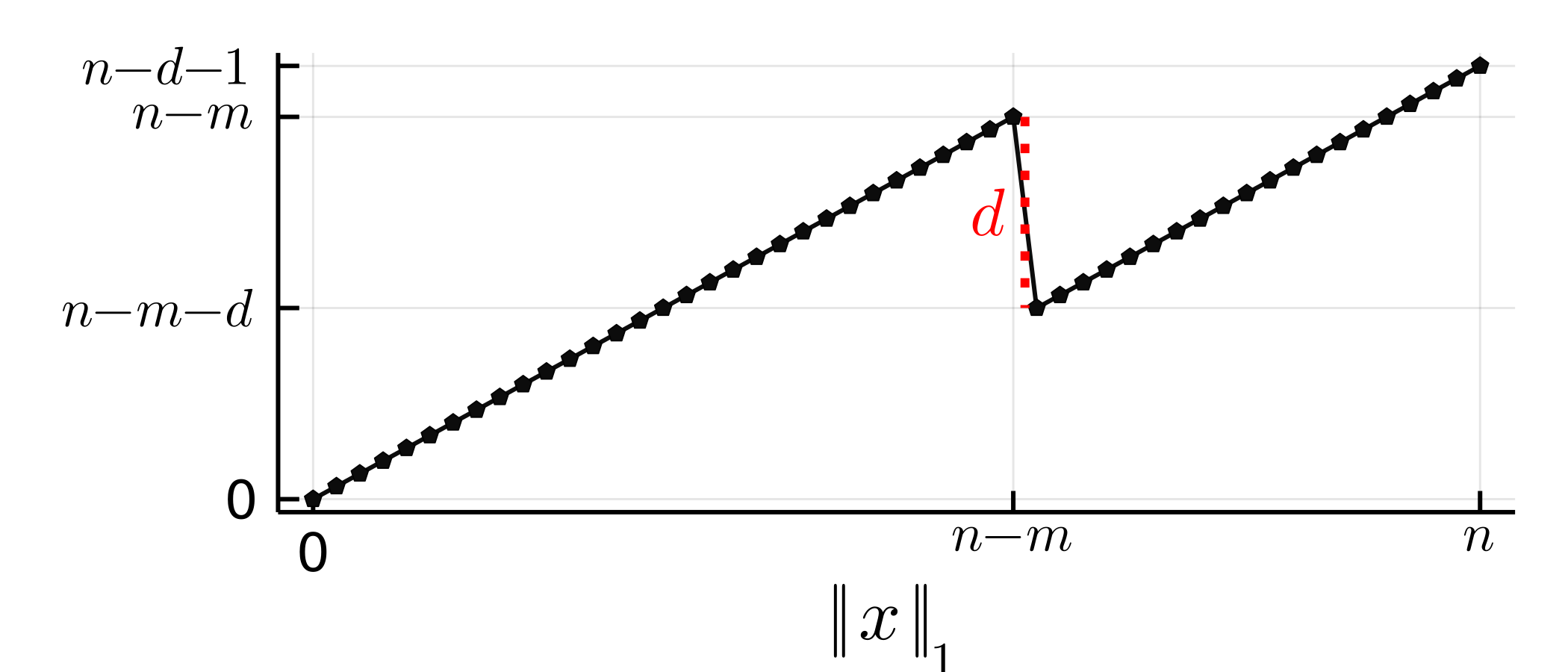
Figure 1. The function $\textsc{Cliff}_{d,m}$.

To the best of our knowledge, the only runtime analysis of the MA on Cliff functions was conducted by (Lissovoi et al., 2023, Theorem 11). On the original $\textsc{Cliff}_{d,m}$ function with fixed $d=m-3/2$, the authors showed a lower bound for the runtime of

$$\min\left\{\frac{1}{2}\cdot\frac{n-m+1}{m-1}\cdot\left(cn/\log n\right)^{m-3/2},n^{\omega(1)}\right\},$$

where $c>0$ is a suitable constant. For super-constant valley widths (and thus cliff heights), this result assures that the runtime of the Metropolis algorithm is super-polynomial. For constant $m$, the $\tilde{\Omega}(n^{m-0.5})$ lower bound is mildly lower than the $\Theta(n^{m})$ runtime of the ${(1+1)}$ EA. So this result leaves some room for a possible advantage from accepting inferior solutions for the restricted case that the valley extends to the global optimum.

On the two slopes of Cliff, the function is essentially equivalent to the classic OneMax benchmark

$$\textsc{OneMax}(x)\coloneqq\|x\|_{1}.$$

Consequently, understanding the MA on OneMax will be crucial for our analysis on Cliff. Intuitively, if the MA is run on Cliff, assuming $m\ll n/2$, it first of all has to optimize a OneMax-like function to reach the cliff, accept the drop to jump down the cliff and then again optimize a OneMax-like function to reach the global optimum. However, it may (and usually will) happen that the MA returns to the cliff point or even points left of the cliff again after having overcome it for the first time.

4. Mathematical Runtime Analysis

4.1. OneMax

As explained above, we start our mathematical analysis with a runtime analysis of the MA on OneMax. This results will be needed in our analysis on Cliff, but it is also interesting in its own right as it very precisely describes the transitions between the different parameter regimes.

Many randomized search heuristics optimize the OneMax function in time $\Theta(n\log n)$. More precisely, a runtime of $(1\pm o(1))n\ln(n)$ is the best performance a heuristic can have which generates offspring from single previous solutions in an unbiased manner (Doerr et al., 2020a). It is easy to see that with a sufficiently small temperature (that is, $\alpha$ sufficiently large), the MA attains this runtime as well. Since in our analysis on Cliff smaller values of $\alpha$ will be necessary to leave the local optimum, we need a runtime analysis also for such parameter values. The only previous work on this question (Jansen and Wegener, 2007) has shown the following three results for the number $T$ of iterations taken to find the optimum:

• If $\alpha\geq\epsilon n$ for any positive constant $\epsilon$, then

  $$E[T]=O(n\log n).$$

• If $\alpha=o(n)$, then

  $$E[T]=\Omega(\alpha 2^{n/3\alpha}).$$

• $E[T]$ is polynomial in $n$ if and only if $\alpha=\Omega(n/\log n)$.

Our main result, see Theorem A.5 below, significantly extends this state of the art. Different from the previous work, it is tight apart from lower order terms for all $\alpha=\omega(\sqrt{n})$ and thus, in particular, for the phase transition between $(1+o(1))n\ln n$ and runtimes exponential in $\frac{n}{\alpha}$.

Moreover, it implies that the best possible runtime of $(1\pm o(1))n\ln n$ is obtained for $\alpha\geq\frac{n}{\ln\ln n}$, which characterizes the optimal parameter settings for the MA on OneMax.

Our result also implies the known result that the runtime is polynomial in $n$ if and only if $\alpha=\Omega(\frac{n}{\log n})$, however, we also make precise the runtime behavior in this critical phase: For all $\alpha=\frac{1}{c}\frac{n}{\ln n}$, the runtime is

$$(1\pm o(1))\frac{1}{c}n^{c+1}(\ln n)^{-1}.$$

Our methods would also allow to prove results for smaller values of $\alpha$, but in the light of the previously shown $\exp(\Omega(n/\alpha))$ lower bound, these appear less interesting and consequently we do not explore this further.

Theorem 4.1.

Let $T$ be the runtime of the MA with $\alpha=\omega(\sqrt{n})$ on OneMax. Then

$$E[T]=(1\pm o(1))n\ln(n)+\mathds{1}_{\alpha\leq n}(1\pm o(1))\alpha e^{n/\alpha}.$$

The proof of our theorem uses state-of-the-art methods for the runtime analysis that were not available at the time of Jansen and Wegener (2007). In particular, we use so-called drift arguments, see Lengler (2020), to show that the MA quickly reaches the equilibrium point of $\kappa=n-\lceil\tfrac{n}{\alpha+1}\rceil$ one-bits in the proof of the following Theorem A.1.

Theorem 4.2.

Let $d(x)$ be the fitness distance (and Hamming distance) of $x$ to the optimum, in other words, the number of zeros in $x$ and $x^{(t)}$ denote the current solution at the end of iteration $t$ (and $x^{(0)}$ the random initial solution). Let $k^{*}=\frac{n}{\alpha+1}$ and $k=\lceil k^{*}\rceil$. Then the first time $T$ such that the Metropolis algorithm with parameter $\alpha$ finds a solution $x^{(T)}$ with $d(x^{(T)})\leq k$ satisfies

$$E[T]\leq\frac{\alpha}{\alpha+1}n(\ln(n)+1).$$

If $k=o(n)$, then we also have $E[T]\geq(1-o(1))n\ln(\frac{n}{k})$.

Proof.

By definition of the algorithm, the probability for reducing the fitness distance from a solution $x$ with $i$ zero-bits is

$$p_{i}^{-}:=\frac{i}{n}$$

and the probability for increasing the distance is

$$p_{i}^{+}:=\frac{n-i}{\alpha n}.$$

Let $D_{t}=d(x^{(t)})$ for convenience. We see that the expected progress in one iteration satisfies

(1) $$E[D_{t}-D_{t+1}\mid D_{t}]=p_{D_{t}}^{-}+\frac{1}{\alpha}\,p_{D_{t}}^{+}=D_{t}\left(\frac{1}{n}+\frac{1}{\alpha n}\right)-\frac{1}{\alpha}\,.$$

To derive a situation with multiplicative drift, we regard a shifted version of the process $(D_{t})$. Let $X_{t}=D_{t}-k^{*}$ for all $t$. By (5), we have

$$E[X_{t}-X_{t+1}\mid X_{t}] =E[D_{t}-D_{t+1}\mid D_{t}]$$

$$=D_{t}\left(\frac{1}{n}+\frac{1}{\alpha n}\right)-\frac{1}{\alpha}$$

$$=\left(X_{t}+\frac{n}{\alpha+1}\right)\left(\frac{1}{n}+\frac{1}{\alpha n}\right)-\frac{1}{\alpha}$$

$$=X_{t}\left(\frac{1}{n}+\frac{1}{\alpha n}\right)=:X_{t}\delta,$$

that is, we have an expected multiplicative progress towards $0$ in the regime $X_{t}\geq 0$ (which is the regime $D_{t}\geq k^{*}$).

To apply the multiplicative drift theorem, we require a process in the non-negative numbers, having zero as target, and such that the smallest positive value is bounded away from zero. For this reason, we define $(Y_{t})$ by $Y_{t}=0$ if $X_{t}<k+1-k^{*}=:y_{\min}$ and $Y_{t}=X_{t}$ otherwise (in other words, for $D_{t}\geq k+1$, the processes $(X_{t})$ and $(Y_{t})$ agree, and we have $Y_{0}=0$ otherwise). Since $(X_{t})$ changes by at most one per step and since $y_{\min}\geq 1$, in an iteration $t$ such that $X_{t}=Y_{t}\geq y_{\min}$ we have $Y_{t+1}\leq X_{t+1}$ and thus $E[Y_{t}-Y_{t+1}\mid Y_{t}]\geq E[X_{t}-X_{t+1}\mid X_{t}]=X_{t}\delta=Y_{t}\delta$, that is, we have the same multiplicative progress. We can thus apply the multiplicative drift theorem from (Doerr et al., 2012) (also found as Theorem 11 in the survey (Lengler, 2020)) and derive that the first time $T$ such that $Y_{T}=0$ satisfies $E[T]\leq\frac{1+\ln(n/y_{\min})}{\delta}\leq\frac{\alpha}{\alpha+1}n(\ln(n)+1)$ as claimed.

For the lower bound, we argue as follows, very similar to the proof of (Jansen and Wegener, 2007, Proposition 5). Let $D_{0}$ be the fitness distance of the initial random search point. We condition momentarily on a fixed outcome of $D_{0}$ that is larger than $k$. Consider in parallel a run of the randomized local search heuristic RLS (Doerr et al., 2020a) on OneMax, starting with a fitness distance of $D_{0}$. Note that this is equivalent to saying that we start a second run of the Metropolis algorithm with parameter $\alpha=\infty$. Denote the fitness distances of this run by $\tilde{D}_{t}$. This is again a Markov chain with one-step changes in $\{-1,0,1\}$, however, with transition probabilities $\tilde{p}_{i}^{-}=p_{i}^{-}$ and $\tilde{p}_{i}^{+}=0\leq p_{i}^{+}$. Consequently, a simple induction shows that $D_{t}$ stochastically dominates $\tilde{D}_{t}$. In particular, the first hitting time $\tilde{T}$ of $k$ of this chain is a lower bound for $T$, both in the stochastic domination sense and in expectation. We therefore analyze $\tilde{T}$. Since $\tilde{D}_{t}$ in each step either decreases by one or remains unchanged, we can simply sum up the waiting times for making a step towards the target, that is, $E[\tilde{T}]=\sum_{i=D_{0}}^{k-1}\frac{1}{p_{i}^{-}}=\sum_{i=D_{0}}^{k-1}\frac{n}{i}=n(H_{D_{0}}-H_{k-1})$, where $H_{m}:=\sum_{i=1}^{m}\frac{1}{i}$ denotes the $m$-th Harmonic number. Using the well-known estimate $\ln(m)\leq H_{m}\leq\ln(m)+1$, we obtain $E[\tilde{T}]\geq n(\ln(D_{0})-\ln(k)-1)$. Recall that this estimate was conditional on a fixed value of $D_{0}$. Since $D_{0}$ follows a binomial distribution with parameters $n$ and $\frac{1}{2}$, we have $D_{0}\geq\frac{n}{2}-n^{3/4}$ with probability $1-o(1)$, and in this case, $E[T\mid D_{0}\geq\frac{n}{2}-n^{3/4}]\geq n(\ln(\frac{n}{2}-n^{3/4}-1)-\ln(k)-1)=(1-o(1))n\ln(\frac{n}{k})$, where the last estimate exploits our assumption $k=o(n)$. Just from the contribution of this case, we obtain $E[T]\geq(1-o(1))E[T\mid D_{0}\geq\frac{n}{2}-n^{3/4}]=(1-o(1))n\ln(\frac{n}{k})$. ∎

Once the number of one-bits has reached at least $\kappa$, it is less likely to flip one of the few remaining zero-bits (which is necessary to make further progress) than to generate and accept an inferior solution. In this region of negative drift, we use a precise Markov chain analysis. This analysis considers the expected transition times $E_{i}$ from the level of $n-i$ to the level of $n-i+1$ one-bits and makes heavy use of the recursion formula

$$E_{i}=\frac{n}{i}+\frac{n-i}{\alpha i}E_{i+1}$$

that is a consequence of the Markov property and the transition probabilities $i/n$ and $\alpha(n-i)/n$ from the level of $n-i$ one-bits to a superior and inferior level, respectively.

We profit here from the fact that the optimization time when starting in an arbitrary solution in the negative drift regime is very close to the optimization time when starting in a solution that is a Hamming neighbor of the optimum. This runtime behavior, counter-intuitive at first sight, is caused by the fact that the apparent advantage of starting with a Hamming neighbor is diminished by that fact that (at least for $\alpha$ not too large) it is much easier to generate and accept an inferior solution than to flip the unique missing bit towards the optimum. We make this precise in the following theorem. Since it does not take additional effort, we formulate and prove this result for a range of starting points $k$ that extends also in the regime of positive drift. In this section, we shall use it only for $\ell=k=\lceil k^{*}\rceil$.

Theorem 4.3.

For all $1\leq\ell\leq\frac{2.5}{1+2.5/\alpha}\frac{n}{\alpha}$, we have

$$E_{1}\leq E_{\ell}^{0}\leq(1+O(\tfrac{\alpha}{n}))E_{1}.$$

To estimate $E_{1}$, we use again elementary Markov arguments, but this time to derive an expression for $E_{1}$ in terms of $E_{\ell}$ for some $\ell$ sufficiently far in the regime with positive drift (Theorem A.3). Being in the positive drift regime, $E_{\ell}$ then can be easily bounded via drift arguments, which gives the final estimate for $E_{1}$ (Corollary A.4).

Theorem 4.4.

Let $\alpha\geq 1$ and $\ell=o(\sqrt{n})$. Let

$$E_{1}^{+}=n\left(\sum_{i=0}^{\ell-1}\left(\frac{n}{\alpha}\right)^{i}\frac{1}{(i+1)!}\right)+\left(\frac{n}{\alpha}\right)^{\ell}\frac{1}{\ell!}E_{\ell+1}.$$

Then $(1-o(1))E_{1}^{+}\leq E_{1}\leq E_{1}^{+}$.

By estimating $E_{\ell}$ for $\ell$ in the positive drift regime, we obtain the following estimate for $E_{1}$, which is tight apart from lower order terms when $\alpha=o(n)$.

Corollary 4.5.

Let $\alpha=\omega(\sqrt{n})$. Then

$$(1-2\exp(-\tfrac{2}{3}\tfrac{n}{\alpha})-o(1))\alpha e^{n/\alpha}\leq E_{1}\leq\alpha e^{n/\alpha}.$$

If $\alpha\geq 2n$, then $E_{1}\leq 2n$.

Proof of Theorem A.5.

Let $k=\lceil\frac{n}{\alpha+1}\rceil$. Let $T_{k}$ be the first time that a solution $x$ with $d(x)\leq k$ is found. By Theorem A.1, we have $E[T_{k}]\leq(1+o(1))n\ln(n)$. Since $\alpha=\omega(1)$ and thus $k=o(n)$, Theorem A.1 also gives the lower bound $E[T_{k}]\geq(1-o(1))n\ln(\frac{n}{k})$.

When $\alpha\geq n-1$, that is, $k=1$, then by Corollary A.4 the remaining expected runtime is $E_{1}=O(n)$. Together with our estimates on $T_{k}$, this shows the claim $E[T]=(1\pm o(1))n\ln(n)$ for this case.

Hence let $\alpha<n-1$ and thus $k\geq 2$. Since $\alpha=\omega(\sqrt{n})$ and we aim at an asymptotic result, we can assume that $n$, and thus $\alpha$, are sufficiently large. Then $k\leq 2\frac{n}{\alpha+1}\leq\frac{2.5}{1+2.5/\alpha}\frac{n}{\alpha}$, that is, $k$ satisfies the assumptions of Theorem A.2. By this theorem, the expectation of the remaining runtime satisfies $E_{k}^{0}=(1+O(\frac{\alpha}{n}))E_{1}$. By Corollary A.4, $E_{1}\leq\alpha e^{n/\alpha}$. This shows an upper bound of $E[T]\leq(1+o(1))n\ln(n)+(1+O(\frac{\alpha}{n}))\alpha e^{n/\alpha}$. For $\alpha\geq\frac{n}{\ln\ln n}$, this is the claimed upper bound $(1+o(1))n\ln(n)$, for $\alpha<\frac{n}{\ln\ln n}$, this is the claimed upper bound $(1\pm o(1))n\ln(n)+(1\pm o(1))\alpha e^{n/\alpha}$.

If remains to show the lower bound for $\alpha<n-1$. If $\alpha\geq\frac{n}{\ln\ln n}$ and thus $k=O(\log\log n)$, the lower bound

$$E[T_{k}] \geq(1-o(1))n\ln(\tfrac{n}{k})$$

$$=(1-o(1))n\ln(n)$$

suffices. For $\alpha<\frac{n}{\ln\ln n}$, we estimate $E[T]\geq E[T_{k}]+E_{k}^{0}\geq E[T_{k}]+E_{1}=(1-o(1))n\ln(\frac{n}{k})+(1-2\exp(-\frac{2}{3}\frac{n}{\alpha})-o(1))\alpha e^{n/\alpha}=(1-o(1))n\ln(\frac{n}{k})+(1-o(1))\alpha e^{n/\alpha}$, again using Theorem A.2 and Corollary A.4. For $\alpha\geq\frac{n}{\ln(n)}$, we have $\ln(\frac{n}{k})=(1-o(1))\ln(n)$ and thus $E[T]\geq(1-o(1))n\ln(n)+(1-o(1))\alpha e^{n/\alpha}$. For $\alpha\leq\frac{n}{\ln(n)}$, we have $n\ln(n)=o(\alpha e^{n/\alpha})$, hence our claimed lower bound is $E[T]\geq(1-o(1))\alpha e^{n/\alpha}$, which follows trivially from the estimate $E[T]\geq(1-o(1))n\ln(\frac{n}{k})+(1-o(1))\alpha e^{n/\alpha}$ just shown. ∎

As an additional insight from the drift analysis, we obtain that a OneMax-value of at least $n-\lceil\frac{n}{\alpha+1}\rceil$ is always obtained very efficiently (in expected time $(1+o(1))n\ln n$ at most). Hence as long as $\alpha=\omega(1)$, an almost optimal solution of fitness $(1-o(1))n$ is found in that time.

4.2. Cliff

We now analyze the runtime of the Metropolis on the generalize class of Cliff functions proposed in this work. Compared to the previous analysis on classic Cliff functions in (Lissovoi et al., 2023), we overcome two additional technical obstacles. The first, obvious one, is that our class of Cliff functions comes with two parameters $m$ and $d$ and the MA has the parameter $\alpha$. In this three-dimensional parameter space, complex interactions appear which make the runtime analysis challenging and the final results complex. The second is that we aim at tighter bounds than those shown in (Lissovoi et al., 2023) and at bounds that are informative also in the super-polynomial regime. For this reason, we cannot assume that $\alpha=\Omega(n/\log n)$ as otherwise the hill-climbing part would be super-polynomial.

Nevertheless, we can describe parameter ranges leading to efficient runtimes, determine whether the runtime depends polynomially or exponentially on the parameters, and achieve rather tight bounds.

Our main result, Theorem 4.6 below, distinguishes between two cases according to the location of the cliff (i. e., the points having $n-m$ one-bits) in relation to the equilibrium point $n-\lceil\frac{n}{\alpha+1}\rceil$ mentioned above w. r. t.  OneMax. In Part 1 of the theorem, the equilibrium point comes after the cliff point (i. e., all points before the cliff have a positive drift), while Part 2 covers the opposite case. Intuitively, the distinction takes into account that overcoming the cliff without falling back before the cliff is especially unlikely if the cliff resides in the negative drift region. In Part 1, the runtime bounds depend crucially on the transition time $E_{m-1}$ from $n-m+1$ to $n-m+2$ one-bits. Intuitively, this term arises since all neighbors of state $n-m+1$ are improving, making a transition back to the cliff point of $n-m$ one-bits likely. Once the MA has reached at least $n-m+2$ one-bits, at least one worsening would have to be a accepted to return to the cliff, which in turn makes it more likely to reach the global optimum from those states.

Theorem 4.6.

Let $T$ be the runtime of the MA with $\alpha=\omega(\sqrt{n})$ on $\textsc{Cliff}_{d,m}$, where $m=o(\sqrt{n})$ and $d\geq 1$. Let $k^{*}\coloneqq\frac{n}{\alpha+1}$ and $\beta\coloneqq\frac{2.5}{1+2.5/\alpha}(n/\alpha)$. Let $E_{m-1}$ denote the first hitting time of a state with $n-m+2$ one-bits from a state with $n-m+1$ one-bits. Then:

1. If $k^{*}<m+1$, then

   $$\mathord{E}\mathord{\left[T\right]} \leq\begin{cases}\left((1+O(\frac{\alpha}{n}))\frac{\left(\frac{n}{\alpha}\right)^{m-2}}{(m-2)!}+1+o(\tfrac{\alpha}{n})\right)E_{m-1}&\mbox{}\\ \hfill{\text{if }m-2\leq\beta,}&\\ \left((1+O(\frac{\alpha}{n}))\frac{\left(\frac{n}{\alpha}\right)^{m-2}}{(m-2)!}+\tfrac{5}{3}+o(\tfrac{\alpha}{n})\right)E_{m-1}&\mbox{}\\ \hfill{\text{if }m-2>\beta},\end{cases}$$

   and

   $$\mathord{E}\mathord{\left[T\right]} \geq\left(1-o(1)\right)\left(\frac{\left(\frac{n}{\alpha}\right)^{m-2}}{(m-2)!}+1\right)E_{m-1},$$

   where

   $$(1-o(1))\frac{n^{2}\alpha^{d-1}}{m(m-1)}\left(\alpha+\frac{n}{m+1}\right)\leq E_{m-1}$$

   $$\leq(1+o(1))\frac{n^{2}\alpha^{d-1}}{m(m-1)}\left(\alpha+\frac{n}{(m+1)\frac{\alpha+1}{\alpha}-n/\alpha}\right).$$

2. If $m+1\leq k^{*}$, then

   $$\left(\frac{1}{\sqrt{2\pi}e^{\alpha/(12n)}}-o(1)\right)\frac{\alpha^{d+2}e^{n/\alpha}}{\sqrt{n/\alpha}}\leq\mathord{E}\mathord{\left[T\right]}$$

   $$\hskip 85.35826pt\leq(1-o(1))\alpha^{d+2}e^{n/\alpha}.$$

The proof of the theorem starts out with similar methods like on OneMax, i. e., drift analysis and estimations of expected transitions times between neighboring states of MA. A big amount of additional complexity has to be introduced to analyze the MA when its search point is around the cliff. Here the MA tends to repeatedly jump down and up the cliff, which has to be handled by careful analyses of random walks. Also, the second case ($m+1\leq k^{*}$) has to be analyzed with different arguments than the first case since the drift at the cliff point switches sign accordingly. Again, the recursive expression for the transition times $E_{i}$ mentioned above plays a central role in this analysis.

We will develop simpler, but weaker bounds for the runtime formulas of the theorem in Subsection 4.3 where we compare the results from the two main theorems in this section.

To compare the Metropolis algorithm with evolutionary algorithms, we now also estimate the optimization time of the ${(1+1)}$ EA on Cliff functions. An expected runtime of $\Theta(n^{m})$ has already been proven in Paixão et al. (2017) for the classic case $d=m-3/2$ and mutation rate $p=\frac{1}{n}$.

In the following theorem, we prove an upper bound on the optimization time of the ${(1+1)}$ EA with general mutation rate $p$ on $\textsc{Cliff}_{d,m}$. Since our main aim is showing that the ${(1+1)}$ EA in many situations is faster than the MA, we prove no lower bounds. We note that for $k$ or $p$ not too large, one could show matching lower bounds with the methods developed in Doerr et al. (2017); Bambury et al. (2021).

Theorem 4.7.

Consider the ${(1+1)}$ EA with general mutation rate $0<p<\frac{1}{2}$ optimizing $\textsc{Cliff}_{d,m}$ with arbitrary $m$ and $1\leq d<m-1$. Then the expected optimization time is at most

$$E[T] \leq p^{-1}(1-p)^{-n+1}(1+\ln n)$$

$$\quad+\binom{m}{\lfloor d\rfloor+2}^{-1}p^{-\lfloor d\rfloor-2}(1-p)^{-n+\lfloor d\rfloor+2}.$$

Any $p$ minimizing this bound satisfies $p\leq\frac{\lfloor d\rfloor+2}{n}$. If $m=O(n^{1/2}/\log n)$ and $p=\frac{\lambda}{n}$ for some $0<\lambda\leq\lfloor d\rfloor+2$, then this bound is $E[T]\leq(1+o(1))\frac{e^{\lambda}}{\lambda^{\lfloor d\rfloor+2}}\binom{m}{\lfloor d\rfloor+2}^{-1}n^{\lfloor d\rfloor+2}$. This latter bound is minimized for $\lambda=\lfloor d\rfloor+2$, which yields

$$E[T]\leq(1+o(1))\binom{m}{\lfloor d\rfloor+2}^{-1}\left(\frac{ne}{\lfloor d\rfloor+2}\right)^{\lfloor d\rfloor+2}.$$

The proof of the theorem uses the well-known fitness-level technique (Wegener, 2001) to analyze the expected time until the ${(1+1)}$ EA reaches the cliff point. Moreover, the same type of arguments is used to analyze the expected time to reach the global optimum after having reached the level of at least $n-m+\lfloor d\rfloor+2$ one-bits, i. e., a level to the right of the cliff having strictly larger fitness than the cliff point. These expected times are essentially covered by the first term in the general bound on $\mathord{E}\mathord{\left[T\right]}$ in the theorem. The second term essentially accounts for the expected time to reach the level $n-m+\lfloor d\rfloor+2$ from the cliff. Additional arguments are used if $d$ is an integer, i. e., the levels of $n-m$ and $n-m+d+1$ one-bits share the same fitness. Here MA can jump back to the cliff point from the level of $n-m+d+1$ one-bits (and in fact such a jump back tends to be more likely than a step increasing the number of one-bits), so a random walk analysis is employed to estimate the time to reach the level of $n-m+d+2$ one-bits for the first time.

4.3. Comparison of MA and ${(1+1)}$ EA

Still considering the Cliff function, we shall now compare the bounds we have obtained for the expected runtime of the MA in Theorem 4.6 with the bounds on the runtime of the ${(1+1)}$ EA from Theorem B.6. To this end, we will first investigate optimal parameter choices for $\alpha$ depending on the Cliff parameters $m$ and $d$ and compare it with the bound for the ${(1+1)}$ EA, both for the standard mutation probability $1/n$ and the optimized one $(\lfloor d\rfloor+2)/n$.

Our bounds on the runtime of MA and ${(1+1)}$ EA are rather precise, but arithmetically complicated and not necessarily tight. Since we want to analyze how much faster the MA can be compared to the ${(1+1)}$ EA, we compute parameter settings for $\alpha$ that make the lower bounds for the MA as small as possible. These minimized lower bounds will be contrasted with the upper bounds for the ${(1+1)}$ EA. Again, we have to distinguish between the two main cases for $m$ in relation to $n$ and $\alpha$ that appear in Theorem 4.6.

Case $\boldmath m+1>\lceil\tfrac{n}{\alpha+1}\rceil$: In this case, corresponding to Part 1 of Theorem 4.6, we have a lower bound on the runtime of the MA of

$$(1-o(1))\left(1+\frac{\left(\frac{n}{\alpha}\right)^{m-2}}{(m-2)!}\right)\frac{n^{2}\alpha^{d}}{m(m-1)}.$$

By computing the derivative of $\alpha^{d}\big{(}1+\frac{\left(\frac{n}{\alpha}\right)^{m-2}}{(m-2)!}\big{)}$, we find that the expression is first decreasing and then increasing in $\alpha$ if $m-2\geq d$. We assume this condition on $d$ now without analyzing the border case $d\in(m-2,m-1)$. Then the bound (up to a factor $1\pm o(1)$) is minimized for $\alpha^{*}=n\left(\frac{m-d-2}{d(m-2)!}\right)^{1/(m-2)}.$ For convenience, we assume $m=\omega(1)$ hereinafter and obtain

$$\alpha^{*}=(1\pm o(1))\frac{en}{m-2}.$$

Plugging this in our lower bound, we have an expected runtime for the MA of at least $(1-o(1))\frac{n^{2}}{m^{2}}\alpha^{d}=(1-o(1))e^{d}\left(\frac{n}{m}\right)^{d+2}.$

By comparison, the bounds for the ${(1+1)}$ EA with the two mutation probabilities $1/n$ and $(\lfloor d\rfloor+2)/n$ are no larger than

$$(1+o(1))e\left(\frac{n(\lfloor d\rfloor+2)}{m}\right)^{\lfloor d\rfloor+2}\text{and }(1+o(1))\left(\frac{ne}{m}\right)^{\lfloor d\rfloor+2},$$

respectively, where we used $\binom{a}{b}\geq(a/b)^{b}$. Hence, if $d$ is not an integer, the bound for the optimized ${(1+1)}$ EA is by a factor $\Theta((n/m)^{\lceil d\rceil-d})$ smaller than for the MA; in the exceptional case of integral $d$, the bound for the MA is by a factor no larger than $(1+o(1))e^{2}$ smaller. The bound for the standard ${(1+1)}$ EA loses at most a factor of order $O(d^{d})$. Note also that $d$ must be a small constant for efficient (polynomial) optimization times anyway. Hence, the optimized MA is not much faster than the standard ${(1+1)}$ EA, while typically the optimized ${(1+1)}$ EA is even faster than the optimized MA.

Intuitively, the value $\alpha^{*}\approx\frac{en}{m}$ says that the equilibrium point $\frac{n}{\alpha+1}$ is around $\frac{m}{e}$, i. e., the cliff is clearly in the positive drift region. Hence, it seems plausible that the true minimal expected runtime of the MA is obtained for $\alpha$ falling into the present case. However, since we do not have a sufficiently precise, global expression for the runtime, we still have to consider the case with the cliff in the negative drift region.

Case $\boldmath m+1\leq\lceil\tfrac{n}{\alpha+1}\rceil$: In this case, corresponding to Part 2 of Theorem 4.6, the bound on the expected runtime of the MA is at least

(2) $$\left(\frac{1}{\sqrt{2\pi}e^{1/12}}-o(1)\right)\frac{\alpha^{d+2}e^{n/\alpha}}{\sqrt{n/\alpha}},$$

where we have used $\alpha\leq n$. For given $n$ and $d$, the latter expression is first decreasing and then increasing in $\alpha$, with the minimum taken at $\alpha^{*}=\tfrac{n}{d+5/2}$. Depending on the integrality of $\tfrac{n}{\alpha+1}$ appearing in the case condition, this choice of $\alpha$ may be slightly too big and violate the general assumption $d<m-1$; however, then $\alpha^{*}\approx\tfrac{n}{d+3}$ can be chosen to minimize the bound while meeting the condition. This will not essentially change the following reasoning. Plugging in $\alpha=\frac{n}{d+5/2}$ in (2) gives a lower bound for the MA of

$$\left(\frac{1}{\sqrt{2\pi}e^{1/12}}-o(1)\right)\left(\frac{ne}{d+5/2}\right)^{d+2}$$

then. The upper bounds for the ${(1+1)}$ EA in Theorem B.6 for mutation probabilities $1/n$ and $(\lfloor d\rfloor+2)/n$ are no larger than

$$(1+o(1))en^{\lceil d\rceil+1}\text{ and }(1+o(1))\left(\frac{ne}{\lfloor d\rfloor+2}\right)^{\lfloor d\rfloor+2},$$

respectively, where we simply estimated $\binom{m}{\lfloor d\rfloor+2}^{-1}\leq 1$. If $d$ is not an integer, the bound for the optimized ${(1+1)}$ EA turns out lower than for the MA by a factor $\Theta((n/d)^{\lceil d\rceil-d})$; if it is an integer, the bound for MA is at most by a constant factor of

$$\sqrt{2\pi}e^{1/12}\left(\frac{d+2.5}{d+2}\right)^{d+2}$$

smaller. Moreover, the bound for the ${(1+1)}$ EA with standard mutation rate is at most by a factor of order $O(d^{d})$ bigger. Altogether, we have arrived at the same conclusions as in the previous case.

5. Experiments

To supplement our theoretical results, we have run the MA, the ${(1+1)}$ EA and a few related algorithms on different instances of the Cliff problem. More precisely, besides the MA with $\alpha\in\{20,30,40\}$ (good values in a preliminary experiment with broader range of $\alpha$), we used the ${(1+1)}$ EA both with the standard mutation probability $1/n$ and the higher mutation probability $\lceil d+1\rceil/n$, the Fast-${(1+1)}$ EA using heavy-tailed mutation from Doerr et al. (2017) (with parameter $\beta=1.5$), and the SD-${(1+1)}$ EA, using stagnation detection, from Rajabi and Witt (2022) (with parameters $R=n^{3}$ and the threshold value $(n/r)^{r}(n/(n-r))^{n-r}\ln(enR)$ for strength $r$). We ran these algorithms on Cliff functions with problem size $n=150$ and problem parameters $d=3$ and growing $m\in\{8,12,16,\dots,32\}$.

The runtimes depicted in Figure 2 show that for all three value of $\alpha$, the MA is clearly slower than the other algorithms (among which the ${(1+1)}$ EA with high mutation rate and Fast ${(1+1)}$ EA performed best).

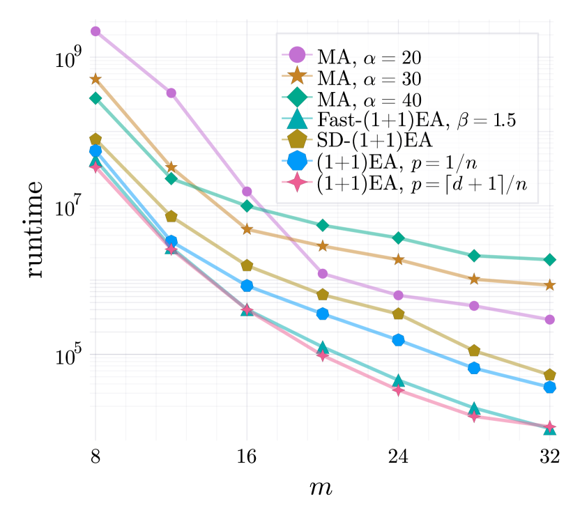
Figure 2. Comparison of MA with ${(1+1)}$ EA and its variants on $\textsc{Cliff}_{m,d}$ for $n=150$, $d=3$ and increasing $m$; averaged over 100 runs.

Since the EAs using global mutation apparently coped well with the valley of low fitness, we also tried the MA with these mutation operators instead of one-bit flips. In this set of experiments, we ran the standard MA, the MA using the standard bit mutation of the ${(1+1)}$ EA with mutation rate $1/n$, and the MA using the heavy-tailed mutation of the Fast-${(1+1)}$ EA, all for $\alpha=20$ (the most promising value for the smaller problem size $n=100$ which we used here). To investigate whether the ability of MA to accept worse search points was relevant, we included the ${(1+1)}$ EA with mutation rate $1/n$ in this comparison. In the runtime results presented in Figure 3, the two global-mutation MAs overall perform better than the standard MA. The ${(1+1)}$ EA might be the overall best choice, only occasionally mildly beaten by the heavy-tailed MA. While these preliminary experiments do not suffice to draw final conclusions, they motivate as future work a closer analysis of MA with global mutation operators.

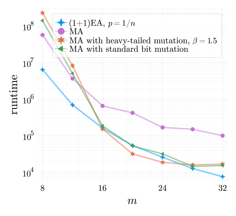
Figure 3. Comparison of ${(1+1)}$ EA and different variants of MA, including global mutation, on $\textsc{Cliff}_{m,d}$ for $n=100$, $\alpha=20$, $d=3$ and increasing $m$; averaged over 50 runs.

6. Conclusions

We have conducted a mathematical runtime analysis of the Metropolis algorithm (MA), a local search algorithm that with positive probability may accept worse solutions, on a generalization of the multimodal Cliff benchmark problem. This problem, which always has a gradient towards the global optimum except for one Hamming level, seems like a canonical candidate where MA can profit from its ability to accept inferior solutions. However, our mathematical runtime analysis has revealed that this intuition is not correct. The simple elitist ${(1+1)}$ EA is for many parameter settings faster than the MA, even for an optimal choice of the temperature parameter of the MA. This failed attempt to explain the effectiveness of the MA raises the question of what is the real reason for the success of the MA in many practical applications.

The comparably good performance of algorithms using global mutation operators suggest to also use the MA with such operators. Our preliminary experimental results show that this can indeed be an interesting idea – backing up these findings with a mathematical runtime analysis is an interesting problem for future research.

A second question of interest is to what extent simulated annealing, that is, the MA with a temperature decreasing over time, can improve the relatively weak performance of the classic MA on Cliff even with optimal choice of the temperature. From our understanding gained in this work, we are slightly pessimistic, mostly because again a relatively small temperature is necessary to reach the local optimum and then diving into the fitness valley is difficult, but definitely a rigorous analysis of this question is necessary to understand this question.

Appendix

In the following two sections, we give detailed analyses including full mathematical proofs of the theorems stated in the Section Mathematical Runtime Analysis of the main paper, dealing with the OneMax and Cliff functions, respectively.

Appendix A Analysis of OneMax – Full Proofs

In this section, we study the performance of the Metropolis algorithm on the OneMax benchmark. OneMax is the possibly best-studied benchmark in the theory of randomized search heuristics. For a given problem size $n\in\mathbb{N}$, the OneMax function is the mapping $f:\{0,1\}^{n}\to\mathbb{N}$ defined by $f(x)=\|x\|_{1}=\sum_{i=1}^{n}x_{i}$ for all $x=(x_{1},\dots,x_{n})\in\{0,1\}^{n}$. This is an easy benchmark representing problems or parts of problems where the gradient points into the direction of the global optimum $x^{*}=(1,\dots,1)$.

It is safe to say that $\Theta(n\log n)$ is a typical runtime of a randomized search heuristic optimizing OneMax. This runtime, more precisely, $(1+o(1))n\ln$ (Doerr et al., 2020a), was proven for the randomized local search heuristic, a randomized hillclimber that flips a single random bit and accepts the new solution if it is at least as good as the previous one. Many simple evolutionary algorithms also solve OneMax in time $\Theta(n\log n)$ with suitable parameters, e.g., the mutation-based ${(\mu+\lambda)}$ EA (Mühlenbein, 1992; Droste et al., 2002; Witt, 2006; Antipov and Doerr, 2021).

It might appear surprising at first that it takes time $\Omega(n\log n)$ to find the correct value of $n$ bits for a simple function like OneMax, where the correct value each bit can be found from the discrete partial derivative at any search point (i.e., by comparing the fitness of the search point and the search point obtained by flipping this bit). The reason is that many randomized search heuristics flip bits chosen at random and then the so-called coupon-collector effect implies that it takes $\Omega(n\log n)$ time until each bit was flipped at least once. It is clear that this problem can be overcome, and an $O(n)$ runtime can be obtained, by flipping the bits in a given order, however, as shown in (Doerr et al., 2010), this can lead to unexpected difficulties when trying to design algorithms that not always flip single bits. Linear runtimes on OneMax have also been obtained via crossover-based EAs (Doerr and Doerr, 2018; Antipov et al., 2020). The black-box complexity of OneMax, that is, the best performance a black-box optimization algorithm can have on the class of all functions isomorphic to OneMax, is $\Theta(n/\log n)$ (Erdős and Rényi, 1963). Despite the fact that these faster performances have been shown for particular algorithms, it still appears appropriate to call $\Theta(n\log n)$ the typical runtime of a general-purpose search heuristic on OneMax. In fact, Lehre and Witt (Lehre and Witt, 2012) have shown that any unary unbiased black-box algorithm, that is, any black-box algorithm that treats the bit positions $1,\dots,n$ and the bit values $0$ and $1$ in a symmetric fashion (unbiasedness) and that creates new solution only from one parent (unary), takes time at least $\Omega(n\log n)$ on OneMax. A precise tight bound of $(1\pm o(1))n\ln n$ was given in (Doerr et al., 2020a).

We now conduct a precise analysis of how the Metropolis algorithm with different values of the parameter $\alpha$ performs on the OneMax problem. The only previous work on this question (Jansen and Wegener, 2007) has shown the following three results for the number $T$ of iterations taken to find the optimum.

• If $\alpha\geq\varepsilon n$ for any positive constant $\varepsilon$, then $E[T]=O(n\log n)$.

• If $\alpha=o(n)$, then $E[T]=\Omega(\alpha 2^{n/3\alpha})$.

• $E[T]$ is polynomial in $n$ if and only if $\alpha=\Omega(n/\log n)$.

This first work clearly shows that a relatively large value of $\alpha$ is necessary to efficiently optimize OneMax.

Our main result (Theorem A.5) is very precise analysis of the runtime of the Metropolis algorithm on OneMax showing that for all $\alpha=\omega(\sqrt{n})$, we have

$$E[T]=(1\pm o(1))n\ln(n)+(1\pm o(1))\alpha\exp(\tfrac{n}{\alpha}).$$

This result covers the most interesting regime describing the transition from polynomial to exponential runtimes. Our methods would also allow to prove results for smaller values of $\alpha$, but in the light of the previously shown $\exp(\Omega(n/\alpha))$ lower bound, these appear less interesting and consequently we do not explore this further.

Different from the previous work, our runtime result is tight apart from lower order terms for all $\alpha=\omega(\sqrt{n})$ and thus, in particular, for the phase transition between $(1+o(1))n\ln n$ and runtimes exponential in $\frac{n}{\alpha}$. From this, we learn that we have a runtime of $(1\pm o(1))n\ln(n)$ if $\alpha\geq\frac{n}{\ln\ln n}$, but that the runtime becomes $\omega(n\log n)$ when $\alpha\leq(1-\varepsilon)\frac{n}{\ln\ln n}$ for any constant $\varepsilon>0$. Recall from above that $(1\pm o(1))n\ln n$ is the best runtime a unary unbiased black-box algorithm can have on OneMax (and in fact any function $f:\{0,1\}^{n}\to\mathbb{R}$ with unique global optimum), so this insight characterizes the optimal parameter settings for the Metropolis algorithm on OneMax.

Our result also implies the known result that the runtime is polynomial in $n$ if and only if $\alpha=\Omega(\frac{n}{\log n})$, however, we also make precise the runtime behavior in this critical phase: For all $\alpha=\frac{1}{c}\frac{n}{\ln n}$, the runtime is $(1\pm o(1))\frac{1}{c}n^{c+1}(\ln n)^{-1}$.

We show this result not only because precise runtime results give a better picture of the performance of an algorithm, but also because our alternative analysis method gives additional insights on where this runtime stems from. In particular, we observe that a OneMax fitness of $\lceil n-\frac{n}{\alpha+1}\rceil$ is always obtained very efficiently (in expected time $(1+o(1))n\ln n$ at most). Hence as long as $\alpha=\omega(1)$, an almost optimal solution of fitness $(1-o(1))n$ is found in that time. A third motivation for this detailed analysis on OneMax is that we need similar arguments in the next section, where we study the performance of the Metropolis algorithm to see how well it copes with local optima.

A.1. Preliminaries and Notation

From the symmetry of the Metropolis algorithm and the OneMax function, it is clear that all search points $x\in\{0,1\}^{n}$ having the same number of ones, that is, the same OneMax value, and thus the same number of zeroes, that is, same distance

$$d(x):=n-\textsc{OneMax}(x)$$

from the optimum, behave equivalently. For this reason, let us, for all $i\in[0..n]$, denote by $L_{i}=\{x\in\{0,1\}^{n}\mid d(x)=i\}$ the set of search points in distance $i$. Since the Metropolis algorithm creates new solutions by flipping single bits, an iteration starting with a solution $x\in L_{i}$ for some $i$ can only end with a solution in $L_{i-1}$, $L_{i}$, or $L_{i+1}$. By definition of the algorithm, the probability for reducing the fitness distance from a solution $x\in L_{i}$ (that is, creating an offspring in $L_{i-1}$) is

$$p_{i}^{-}:=\frac{i}{n}$$

and the probability for increasing the distance (that is, creating an offspring in $L_{i+1}$ and accepting it as new solution) is

$$p_{i}^{+}:=\frac{n-i}{\alpha n}.$$

We note that this notation is different from the one used in (Jansen and Wegener, 2007), where the notation was based on the fitness and not on the distance. Hence our $p_{i}^{+}$ equals the $p_{n-i}^{-}$ used there. We prefer to work with the distance since the more critical part of the optimization process is close to the optimum.

With the transition probabilities just defined, we can use simple Markov chain arguments to, in principle, compute the expected runtime. For $i\geq j$, denote by $E_{i}^{j}$ the expected time the Metropolis algorithm (with some given parameter $\alpha$ suppressed in this notation) takes to find a solution in $L_{j}$ when started with a solution in $L_{i}$. We abbreviate $E_{i}=E_{i}^{i-1}$. Then, by elementary properties of Markov processes,

(3) $$E_{i}^{j}=\sum_{\ell=i}^{j+1}E_{\ell}.$$

From the one-step equation $E_{i}=1+p_{i}^{+}(E_{i+1}+E_{i})+(1-p_{i}^{+}-p_{i}^{-})E_{i}$, we derive the following equation, which was also used in (Jansen and Wegener, 2007).

(4) $$E_{i}=\frac{1}{p_{i}^{-}}+\frac{p_{i}^{+}}{p_{i}^{-}}E_{i+1}.$$

The analysis of the runtime of the Metropolis algorithm on OneMax in (Jansen and Wegener, 2007) was solely based on the above two equations (with, of course, non-trivial estimates of the arising sums). In this work, we partially take a different route by separately analyzing the part of the process in which the algorithm has a positive expected fitness gain per iteration. This is when the fitness distance is still large and thus is it easy to find improving solutions. In this part of the process, we can conveniently use multiplicative drift analysis, a tool presented a few years after (Jansen and Wegener, 2007). For the remainder of the process, we use arguments similar to those in (Jansen and Wegener, 2007), however, we profit from the fact that we need to cover only a smaller range of fitness levels.

A.2. Pseudo-linear Time in the Regime with Positive Drift

We start our analysis with the part of the process where the expected progress per iteration is positive. We recall that we denote by $d(x)$ the fitness distance (and Hamming distance) of $x$ to the optimum, in other words, the number of zeros in $x$. Recalling that $x^{(t)}$ denotes the current solution at the end of iteration $t$ (and $x^{(0)}$ the random initial solution), and defining $D_{t}=d(x^{(t)})$ for convenience, we see that the expected progress in one iteration satisfies

(5) $$E[D_{t}-D_{t+1}\mid D_{t}]=p_{D_{t}}^{-}+\frac{1}{\alpha}\,p_{D_{t}}^{+}=\frac{D_{t}}{n}-\frac{n-D_{t}}{\alpha n}=D_{t}\left(\frac{1}{n}+\frac{1}{\alpha n}\right)-\frac{1}{\alpha}\,.$$

In particular, the expected progress is positive when $D_{t}>\frac{n}{\alpha+1}=:k^{*}$ and negative when $D_{t}<k^{*}$. An expected progress towards a target can be translated into estimates on the hitting time of this target, usually via so-called drift theorems (Lengler, 2020), and this is our approach to show the following result.

Theorem A.1.

Let $k^{*}=\frac{n}{\alpha+1}$ and $k=\lceil k^{*}\rceil$. Then the first time $T$ such that the Metropolis algorithm with parameter $\alpha$ finds a solution $x^{(T)}$ with $d(x^{(T)})\leq k$ satisfies

$$E[T]\leq\frac{\alpha}{\alpha+1}n(\ln(n)+1).$$

If $k=o(n)$, then we also have $E[T]\geq(1-o(1))n\ln(\frac{n}{k})$.

Proof.

To derive a situation with multiplicative drift, we regard a shifted version of the process $(D_{t})$. Let $X_{t}=D_{t}-k^{*}$ for all $t$. By (5), we have

$$E[X_{t}-X_{t+1}\mid X_{t}] =E[D_{t}-D_{t+1}\mid D_{t}]$$

$$=D_{t}\left(\frac{1}{n}+\frac{1}{\alpha n}\right)-\frac{1}{\alpha}$$

$$=\left(X_{t}+\frac{n}{\alpha+1}\right)\left(\frac{1}{n}+\frac{1}{\alpha n}\right)-\frac{1}{\alpha}$$

$$=X_{t}\left(\frac{1}{n}+\frac{1}{\alpha n}\right)=:X_{t}\delta,$$

that is, we have an expected multiplicative progress towards $0$ in the regime $X_{t}\geq 0$ (which is the regime $D_{t}\geq k^{*}$).

To apply the multiplicative drift theorem, we require a process in the non-negative numbers, having zero as target, and such that the smallest positive value is bounded away from zero. For this reason, we define $(Y_{t})$ by $Y_{t}=0$ if $X_{t}<k+1-k^{*}=:y_{\min}$ and $Y_{t}=X_{t}$ otherwise (in other words, for $D_{t}\geq k+1$, the processes $(X_{t})$ and $(Y_{t})$ agree, and we have $Y_{0}=0$ otherwise). Since $(X_{t})$ changes by at most one per step and since $y_{\min}\geq 1$, in an iteration $t$ such that $X_{t}=Y_{t}\geq y_{\min}$ we have $Y_{t+1}\leq X_{t+1}$ and thus $E[Y_{t}-Y_{t+1}\mid Y_{t}]\geq E[X_{t}-X_{t+1}\mid X_{t}]=X_{t}\delta=Y_{t}\delta$, that is, we have the same multiplicative progress. We can thus apply the multiplicative drift theorem from (Doerr et al., 2012) (also found as Theorem 11 in the survey (Lengler, 2020)) and derive that the first time $T$ such that $Y_{T}=0$ satisfies $E[T]\leq\frac{1+\ln(n/y_{\min})}{\delta}\leq\frac{\alpha}{\alpha+1}n(\ln(n)+1)$ as claimed.

For the lower bound, we argue as follows, very similar to the proof of (Jansen and Wegener, 2007, Proposition 5). Let $D_{0}$ be the fitness distance of the initial random search point. We condition momentarily on a fixed outcome of $D_{0}$ that is larger than $k$. Consider in parallel a run of the randomized local search heuristic RLS (Doerr et al., 2020a) on OneMax, starting with a fitness distance of $D_{0}$. Note that this is equivalent to saying that we start a second run of the Metropolis algorithm with parameter $\alpha=\infty$. Denote the fitness distances of this run by $\tilde{D}_{t}$. This is again a Markov chain with one-step changes in $\{-1,0,1\}$, however, with transition probabilities $\tilde{p}_{i}^{-}=p_{i}^{-}$ and $\tilde{p}_{i}^{+}=0\leq p_{i}^{+}$. Consequently, a simple induction shows that $D_{t}$ stochastically dominates $\tilde{D}_{t}$. In particular, the first hitting time $\tilde{T}$ of $k$ of this chain is a lower bound for $T$, both in the stochastic domination sense and in expectation. We therefore analyze $\tilde{T}$. Since $\tilde{D}_{t}$ in each step either decreases by one or remains unchanged, we can simply sum up the waiting times for making a step towards the target, that is, $E[\tilde{T}]=\sum_{i=D_{0}}^{k-1}\frac{1}{p_{i}^{-}}=\sum_{i=D_{0}}^{k-1}\frac{n}{i}=n(H_{D_{0}}-H_{k-1})$, where $H_{m}:=\sum_{i=1}^{m}\frac{1}{i}$ denotes the $m$-th Harmonic number. Using the well-known estimate $\ln(m)\leq H_{m}\leq\ln(m)+1$, we obtain $E[\tilde{T}]\geq n(\ln(D_{0})-\ln(k)-1)$. Recall that this estimate was conditional on a fixed value of $D_{0}$. Since $D_{0}$ follows a binomial distribution with parameters $n$ and $\frac{1}{2}$, we have $D_{0}\geq\frac{n}{2}-n^{3/4}$ with probability $1-o(1)$, and in this case, $E[T\mid D_{0}\geq\frac{n}{2}-n^{3/4}]\geq n(\ln(\frac{n}{2}-n^{3/4}-1)-\ln(k)-1)=(1-o(1))n\ln(\frac{n}{k})$, where the last estimate exploits our assumption $k=o(n)$. Just from the contribution of this case, we obtain $E[T]\geq(1-o(1))E[T\mid D_{0}\geq\frac{n}{2}-n^{3/4}]=(1-o(1))n\ln(\frac{n}{k})$. ∎

We note that there is a non-vanishing gap between our upper and lower bound in the theorem above when $k=n^{\Omega(1)}$. The reason, most likely, is the argument used in the lower bound proof that the Metropolis algorithm cannot be faster than randomized local search, which ignores any negative effect of accepting inferior solutions. For our purposes, the theorem above is sufficient, since for all but very large values of $\alpha$ (where the gap is negligible) the runtime of the Metropolis algorithm is dominated by the second part of the optimization process starting from a solution $x$ with $d(x)=k$. The reason why we could not prove a tighter bound for all values of $\alpha$ is that the existing multiplicative drift theorems for lower bounds, e.g., Theorem 2.2 in (Witt, 2013) or Theorem 3.7 in (Doerr et al., 2020b), either are not applicable to our process or necessarily lead to a constant-factor gap to the upper bound obtained from multiplicative drift. Applying the variable drift theorem from (Doerr et al., 2011) to the process $Z_{t}=\min\{Y_{s}\mid s\leq t\}$ appears to be a promising way to overcome these difficulties, but since we do not need such a precise bound, we do not follow this route any further.

A.3. Progress Starting the Equilibrium Point

In the regime with negative drift, we use elementary Markov chain arguments to estimate runtimes. We profit here from the fact that the optimization time when starting in an arbitrary solution in the negative drift regime is very close to the optimization time when starting in a solution that is a Hamming neighbor of the optimum. This runtime behavior, counter-intuitive at first sight, is caused by the fact that the apparent advantage of starting with a Hamming neighbor is diminished by that fact that (at least for $\alpha$ not too large) it is much easier to generate and accept an inferior solution than to flip the unique missing bit towards the optimum. We make this precise in the following theorem. Since it does not take additional effort, we formulate and prove this result for a range of starting points $k$ that extends also in the regime of positive drift. In this section, we shall use it only for $\ell=k=\lceil k^{*}\rceil$.

Theorem A.2.

For all $1\leq\ell\leq\frac{2.5}{1+2.5/\alpha}\frac{n}{\alpha}$, we have

$$E_{1}\leq E_{\ell}^{0}\leq(1+O(\tfrac{\alpha}{n}))E_{1}.$$

Proof.

By equation (4) and the values for $p_{i}^{+},p_{i}^{-}$ computed earlier, we see that

(6) $$E_{i}=\frac{n}{i}+\frac{n-i}{\alpha i}E_{i+1},$$

for all $i\in[1..n-1]$. By omitting the first summand, we obtain $E_{i+1}\leq\frac{\alpha i}{n-i}E_{i}$, and an elementary induction yields $E_{j+1}\leq\alpha^{j}\frac{1\cdot 2\dots j}{(n-j)\dots(n-1)}E_{1}$ for all $j\in[1..n-1]$. Using the estimate $j!\leq 3\sqrt{j}(\frac{j}{e})^{j}$ stemming from a sharp version of Stirling’s formula due to Robbins (Robbins, 1995) (also stated as Theorem 1.4.10 in (Doerr, 2020)), we estimate, for $j\in[1..\ell]$,

$$\alpha^{j}\frac{1\cdot 2\dots j}{(n-j)\dots(n-1)} \leq 3\frac{\alpha}{n-1}j^{3/2}\left(\frac{\alpha(j-1)}{e(n-j)}\right)^{j-1}$$

$$\leq 3\frac{\alpha}{n-1}j^{3/2}\left(\frac{\alpha\ell}{e(n-\ell)}\right)^{j-1}$$

$$\leq 3\frac{\alpha}{n-1}j^{3/2}\left(\tfrac{2.5}{e}\right)^{j-1},$$

where we note that our assumption $\ell\leq\frac{2.5}{1+2.5/\alpha}\frac{n}{\alpha}$ is equivalent to $\frac{\alpha\ell}{e(n-\ell)}\leq\frac{2.5}{e}$.

By (3), we have

$$E_{\ell}^{0} =E_{1}+\sum_{j=1}^{\ell-1}E_{j+1}$$

$$\leq E_{1}+\sum_{j=1}^{\ell-1}\alpha^{j}\frac{1\cdot 2\dots j}{(n-j)\dots(n-1)}E_{1}$$

$$\leq E_{1}+\sum_{j=1}^{\ell-1}3\frac{\alpha}{n-1}j^{3/2}\left(\tfrac{2.5}{e}\right)^{j-1}E_{1}$$

$$=(1+O(\tfrac{\alpha}{n}))E_{1},$$

where we exploited that the series $\sum_{j=1}^{\infty}j^{A}B^{j}$ converges for all constants $A\in\mathbb{R}$ and $b\in(0,1)$. Note that the first line in this set of equations also shows our elementary lower bound $E_{\ell}^{0}\geq E_{1}$. ∎

From Theorems A.1 and A.2, both applied with $k=\lceil k^{*}\rceil$, we know the runtime of the Metropolis algorithm on OneMax except that we do not yet understand $E_{1}$. This is what we do now.

A.4. Estimating $E_{1}$

To estimate $E_{1}$, we use again elementary Markov arguments, but this time to derive an expression for $E_{1}$ in terms of $E_{\ell}$ for some $\ell$ sufficiently far in the regime with positive drift (Theorem A.3). Being in the positive drift regime, $E_{\ell}$ then can be easily bounded via drift arguments, which gives the final estimate for $E_{1}$ (Corollary A.4).

Theorem A.3.

Let $\alpha\geq 1$ and $\ell=o(\sqrt{n})$. Let

$$E_{1}^{+}=n\left(\sum_{i=0}^{\ell-1}\left(\frac{n}{\alpha}\right)^{i}\frac{1}{(i+1)!}\right)+\left(\frac{n}{\alpha}\right)^{\ell}\frac{1}{\ell!}E_{\ell+1}.$$

Then $(1-o(1))E_{1}^{+}\leq E_{1}\leq E_{1}^{+}$.

Proof.

We first show that for all $\ell\in[0..n-1]$, we have

(7) $$E_{1}=\sum_{i=0}^{\ell-1}\frac{n\cdot(n-1)\dots(n-i)}{\alpha^{i}(i+1)!}+\frac{(n-1)\dots(n-\ell)}{\alpha^{\ell}\ell!}E_{\ell+1}.$$

This is trivially true for $\ell=0$ (when using the convention that an empty sum evaluates to zero and an empty product evaluates to one). Assume now that equation (7) is true for some $\ell\in[0..n-2]$. Together with equation (6), we compute

$$E_{1} =\sum_{i=0}^{\ell-1}\frac{n\cdot(n-1)\dots(n-i)}{\alpha^{i}(i+1)!}+\frac{(n-1)\dots(n-\ell)}{\alpha^{\ell}\ell!}E_{\ell+1}$$

$$=\sum_{i=0}^{\ell-1}\frac{n\cdot(n-1)\dots(n-i)}{\alpha^{i}(i+1)!}+\frac{(n-1)\dots(n-\ell)}{\alpha^{\ell}\ell!}\left(\frac{n}{\ell+1}+\frac{n-(\ell+1)}{\alpha(\ell+1)}E_{\ell+2}\right)$$

$$=\sum_{i=0}^{\ell}\frac{n\cdot(n-1)\dots(n-i)}{\alpha^{i}(i+1)!}+\frac{(n-1)\dots(n-(\ell+1))}{\alpha^{\ell+1}(\ell+1)!}E_{\ell+2},$$

which shows the equation also for $\ell+1$. By induction, the equation holds for all $\ell\in[0..n-1]$.

From equation (7), we immediately obtain $E_{1}\leq E_{1}^{+}$. For $i=o(\sqrt{n})$, we estimate $(n-1)\dots(n-i)=n^{i}\prod_{j=1}^{i}(1-\frac{i}{n})\geq n^{i}(1-\frac{1}{n}\sum_{j=1}^{i}j)=n^{i}(1-\frac{i(i-1)}{2n})=n^{i}(1-o(1))$, where the inequality uses an elementary generalization of Bernoulli’s inequality sometimes called Weierstrass inequality (see, e.g., (Doerr, 2020, Lemma 1.4.8)). This shows the lower bound $E_{1}\geq(1-o(1))E_{1}^{+}$. ∎

By estimating $E_{\ell}$ for $\ell$ in the positive drift regime, we obtain the following estimate for $E_{1}$, which is tight apart from lower order terms when $\alpha=o(n)$.

Corollary A.4.

Let $\alpha=\omega(\sqrt{n})$. Then

$$(1-2\exp(-\tfrac{2}{3}\tfrac{n}{\alpha})-o(1))\alpha e^{n/\alpha}\leq E_{1}\leq\alpha e^{n/\alpha}.$$

If $\alpha\geq 2n$, then $E_{1}\leq 2n$.

Proof.

Let $\ell=\lceil 3\frac{n}{\alpha}\rceil$. Since $\ell=o(\sqrt{n})$, we can use Theorem A.3 with this $\ell$ to estimate $E_{1}$. Let $X$ denote a random variable following a Poisson distribution with parameter $\lambda:=\frac{n}{\alpha}$. Then

$$n\left(\sum_{i=0}^{\ell-1}\left(\frac{n}{\alpha}\right)^{i}\frac{1}{(i+1)!}\right) =\alpha\left(\sum_{i=0}^{\ell-1}\frac{\lambda^{i+1}}{(i+1)!}\right)$$

$$=\alpha e^{\lambda}\left(\sum_{i=0}^{\ell}\frac{\lambda^{i}e^{-\lambda}}{i!}-e^{-\lambda}\right)$$

$$=\alpha e^{\lambda}\left(\Pr[X\leq\ell]-e^{-\lambda}\right).$$

To estimate the second summand in Theorem A.3, we first note that $(\frac{n}{\alpha})^{\ell}\frac{1}{\ell!}\leq(\frac{ne}{\ell\alpha})^{\ell}\leq(\frac{e}{3})^{3\lambda}$ follows from the estimate $\ell!\geq(\frac{\ell}{e})^{\ell}$. To bound $E_{\ell+1}$, we observe from equation (5) that the drift of the fitness distance $D_{t}$, whenever $D_{t}\geq\ell+1$, satisfies $E[D_{t}-D_{t+1}]=D_{t}(\frac{1}{n}+\frac{1}{\alpha n})-\frac{1}{\alpha}\geq\frac{\ell+1}{n}-\frac{1}{\alpha}\geq\frac{2}{\alpha}$, using $\ell\geq 3\frac{n}{\alpha}$ in the last estimate. Consequently, we have an additive drift of at least $\frac{2}{\alpha}$ for $D_{t}\in[\ell+1..n]$, and thus the additive drift theorem of He and Yao (He and Yao, 2001) (also found as Theorem 2.3.1 in (Lengler, 2020)) yields that the expected time it takes to reach a $D_{t}$ value of $\ell$ when starting in $\ell+1$ is at most $E_{\ell+1}\leq\frac{\alpha}{2}$.

Putting these three estimates together, we obtain an upper bound of

$$E_{1} \leq n\left(\sum_{i=0}^{\ell-1}\left(\frac{n}{\alpha}\right)^{i}\frac{1}{(i+1)!}\right)+\left(\frac{n}{\alpha}\right)^{\ell}\frac{1}{\ell!}E_{\ell+1}$$

$$\leq\alpha e^{\lambda}\left(\Pr[X\leq\ell]-e^{-\lambda}\right)+\left(\frac{e}{3}\right)^{3\lambda}\cdot\frac{\alpha}{2}\leq\alpha e^{\lambda}.$$

For the lower bound, we note that a Poisson random variable $Z$ with parameter $\lambda$ satisfies the Chernoff-type bound $\Pr[Z\geq\lambda+\gamma]\leq\exp(-\frac{\gamma^{2}}{2(\lambda+\gamma)})$ for all $\gamma\geq 0$, see (Boucheron et al., 2013, Section 2.2). Consequently, with $\gamma=2\lambda$, we obtain $\Pr[X\leq\ell]\geq 1-\exp(-\frac{2}{3}\lambda)$. This gives a lower bound of

$$E_{1} \geq(1-o(1))n\left(\sum_{i=0}^{\ell-1}\left(\frac{n}{\alpha}\right)^{i}\frac{1}{(i+1)!}\right)$$

$$\geq(1-o(1))\alpha e^{\lambda}\left(\Pr[X\leq\ell]-e^{-\lambda}\right)$$

$$\geq(1-\exp(-\tfrac{2}{3}\lambda)-\exp(-\lambda)-o(1))\alpha e^{\lambda}.$$

For the case $\alpha\geq 2n$, we use again the additive drift argument. Whenever $D_{t}\geq 1$, we have $E[D_{t}-D_{t+1}\mid D_{t}]=D_{t}(\frac{1}{n}+\frac{1}{\alpha n})-\frac{1}{\alpha}\geq\frac{1}{n}-\frac{1}{\alpha}\geq\frac{1}{2n}$. Hence the additive drift theorem bounds the expected time $E_{1}$ to reach $D_{t}=0$ starting from $D_{t}=1$ by $1/\frac{1}{2n}=2n$. ∎

A.5. A Tight Estimate for the Total Optimization Time

From the partial results proven so far, we now obtain an estimate for the total runtime that is tight apart from lower order terms.

Theorem A.5.

Let $T$ be the runtime of the Metropolis algorithm with parameter $\alpha$ on the OneMax function defined on bit strings of length $n$. Let $\alpha=\omega(\sqrt{n})$. Then

$$E[T]=(1\pm o(1))n\ln(n)+{\mathds{1}}_{\alpha\leq n}(1\pm o(1))\alpha e^{n/\alpha}.$$

Proof.

Let $k=\lceil\frac{n}{\alpha+1}\rceil$. Let $T_{k}$ be the first time that a solution $x$ with $d(x)\leq k$ is found. By Theorem A.1, we have $E[T_{k}]\leq(1+o(1))n\ln(n)$. Since $\alpha=\omega(1)$ and thus $k=o(n)$, Theorem A.1 also gives the lower bound $E[T_{k}]\geq(1-o(1))n\ln(\frac{n}{k})$.

When $\alpha\geq n-1$, that is, $k=1$, then by Corollary A.4 the remaining expected runtime is $E_{1}=O(n)$. Together with our estimates on $T_{k}$, this shows the claim $E[T]=(1\pm o(1))n\ln(n)$ for this case.

Hence let $\alpha<n-1$ and thus $k\geq 2$. Since $\alpha=\omega(\sqrt{n})$ and we aim at an asymptotic result, we can assume that $n$, and thus $\alpha$, are sufficiently large. Then $k\leq 2\frac{n}{\alpha+1}\leq\frac{2.5}{1+2.5/\alpha}\frac{n}{\alpha}$, that is, $k$ satisfies the assumptions of Theorem A.2. By this theorem, the expectation of the remaining runtime satisfies $E_{k}^{0}=(1+O(\frac{\alpha}{n}))E_{1}$. By Corollary A.4, $E_{1}\leq\alpha e^{n/\alpha}$. This shows an upper bound of $E[T]\leq(1+o(1))n\ln(n)+(1+O(\frac{\alpha}{n}))\alpha e^{n/\alpha}$. For $\alpha\geq\frac{n}{\ln\ln n}$, this is the claimed upper bound $(1+o(1))n\ln(n)$, for $\alpha<\frac{n}{\ln\ln n}$, this is the claimed upper bound $(1\pm o(1))n\ln(n)+(1\pm o(1))\alpha e^{n/\alpha}$.

If remains to show the lower bound for $\alpha<n-1$. If $\alpha\geq\frac{n}{\ln\ln n}$ and thus $k=O(\log\log n)$, the lower bound $E[T_{k}]\geq(1-o(1))n\ln(\frac{n}{k})=(1-o(1))n\ln(n)$ suffices. For $\alpha<\frac{n}{\ln\ln n}$, we estimate $E[T]\geq E[T_{k}]+E_{k}^{0}\geq E[T_{k}]+E_{1}=(1-o(1))n\ln(\frac{n}{k})+(1-2\exp(-\frac{2}{3}\frac{n}{\alpha})-o(1))\alpha e^{n/\alpha}=(1-o(1))n\ln(\frac{n}{k})+(1-o(1))\alpha e^{n/\alpha}$, again using Theorem A.2 and Corollary A.4. For $\alpha\geq\frac{n}{\ln(n)}$, we have $\ln(\frac{n}{k})=(1-o(1))\ln(n)$ and thus $E[T]\geq(1-o(1))n\ln(n)+(1-o(1))\alpha e^{n/\alpha}$. For $\alpha\leq\frac{n}{\ln(n)}$, we have $n\ln(n)=o(\alpha e^{n/\alpha})$, hence our claimed lower bound is $E[T]\geq(1-o(1))\alpha e^{n/\alpha}$, which follows trivially from the estimate $E[T]\geq(1-o(1))n\ln(\frac{n}{k})+(1-o(1))\alpha e^{n/\alpha}$ just shown. ∎

Appendix B Analysis of Cliff – Full Proofs

We now examine how the Metropolis algorithm behaves when optimizing a function with a local optimum. Two well-established and well-studied benchmark functions to model situations with local optima are Jump (Droste et al., 2002) and Cliff (Jägersküpper and Storch, 2007). In this research, we investigate the Metropolis algorithm on Cliff instead of Jump for two primary reasons. Firstly, on Jump functions, since the difference between the fitness of the local optimum and its neighbors is of order $n$, it is unlikely that the algorithm accepts such a fitness decrease. Also, the deceptive valley in the function Jump does not allow the search to get far from the local optimum because of accepting all improvements. We refer the interested reader to (Lissovoi et al., 2019, Theorem 13) for a lower bound on the optimization time of Metropolis on Jump. We should mention that the authors in (Oliveto et al., 2018) also studied the Metropolis algorithm on the function so-called Valley, which is a multimodal problem containing both increasing and decreasing valleys.

In contrast to Jump functions, for Cliff functions the valley of low fitness is more shallow and the fitness inside the valley is not deceptive, that is, the gradient is pointing towards the optimum. These properties could let them appear like an easy optimization problem for the Metropolis algorithm, but as our precise analysis for the full spectrum of temperatures will show, this is not true.

Cliff functions were originally defined with only one parameter determining the distance of the local optimum from the global optimum (Jägersküpper, 2007). However, since the Metropolis algorithm is sensitive to function values when it accepts worse solutions, we are interested in analyzing different depths for the valley in the fitness function. That is why we define an additional parameter to express the depth of the cliff.

Let again $n\in\mathbb{N}$ denote the problem size. As before, we shall usually suppress this parameter from our notation. Let $m\in\mathbb{N}_{\geq 1}$ and $d\in\mathbb{R}_{>0}$ such that $m<n$ and $d<m-1$. Then the function $\textsc{Cliff}_{d,m}$ is increasing as the number of one-bits of the argument increases except for the points with $n-m$ one-bits, where the fitness decreases sharply by $d$ if we add one more one-bit to the search point. Formally,

$$\textsc{Cliff}_{d,m}(x)\coloneqq\left\{\begin{array}[]{ll}\|x\|_{1}&\mbox{if }\|x\|_{1}\leq n-m,\\ \|x\|_{1}-d-1&\mbox{otherwise}.\end{array}\right.$$

See Figure 4 for a graphical sketch. Note that the original cliff function can be obtained with fixed parameter $d=m-3/2$.

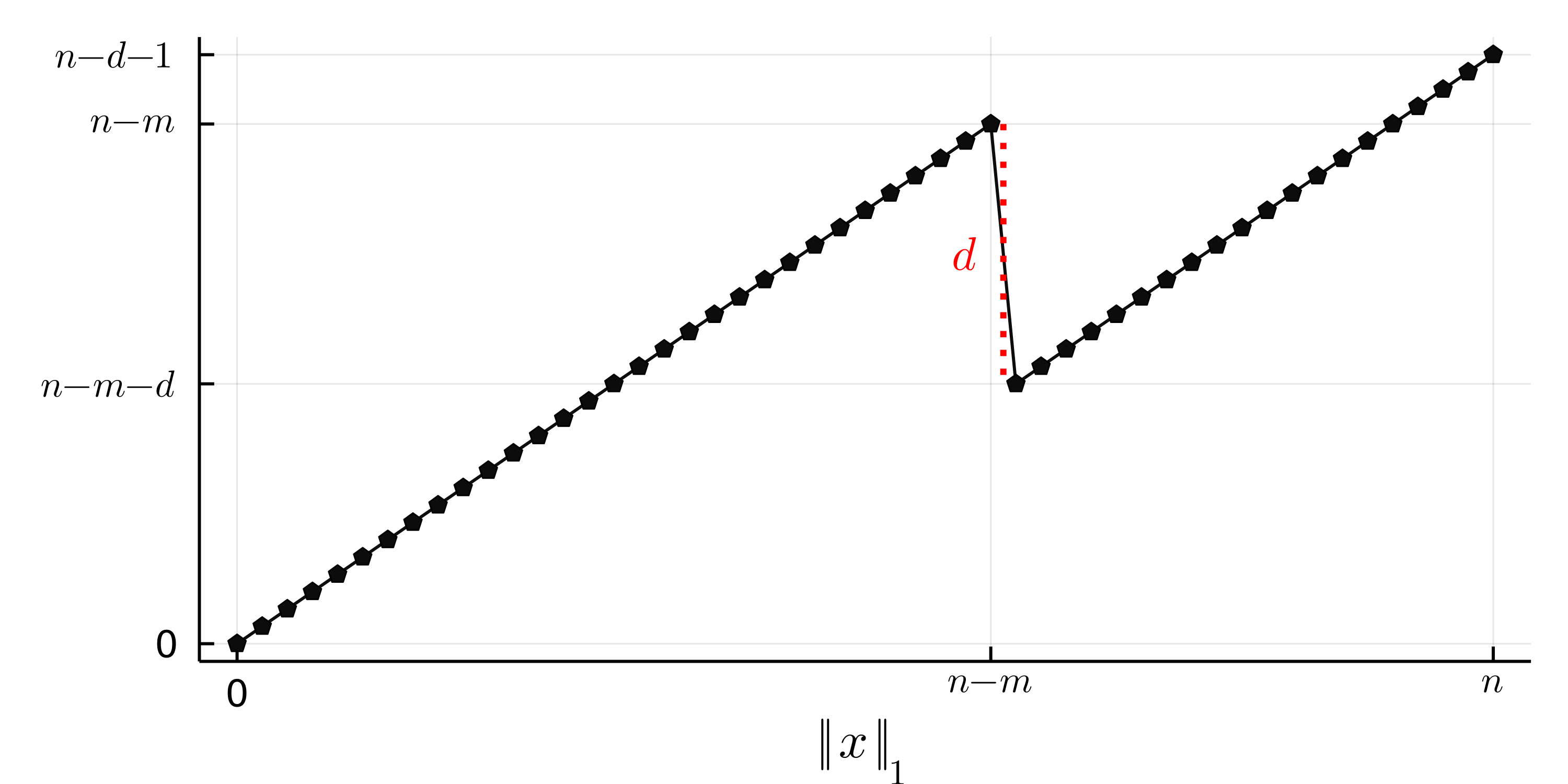
Figure 4. The function $\textsc{Cliff}_{d,m}$.

To the best of our knowledge, the only available analysis of the Metropolis Algorithm on Cliff functions is conducted in (Lissovoi et al., 2019, Theorem 10). On $\textsc{Cliff}_{d,m}$ with fixed $d=m-3/2$, the authors show a lower bound of

$$\min\left\{\frac{1}{2}\cdot\frac{n-m+1}{m-1}\cdot\left(n/\log n\right)^{m-3/2},n^{\omega(1)}\right\}$$

for some $\alpha\geq 1$.

In this paper, we are interested in more rigorous bounds for the optimization time and a better understanding of the impact of two parameters $d$ and $m$, i. e., the depth and the local of the cliff on the runtime.

We recall some definitions used in Subsection A.1. Let $L_{i}$ be the set of search points with $i$ zero-bits, i. e., $L_{i}\coloneqq\{x\in\{0,1\}^{n}\mid n-\|x\|_{1}=i\}$. For $j<i$, let $E_{i}^{j}$ be the expected number of iterations the Metropolis algorithm spends to find a solution in $L_{j}$ when started with a solution in $L_{i}$. We write $E_{i}=E_{i}^{i-1}$. By the distance $d(x)$ of a search point $x$ we understand the Hamming distance to the global optimum $1^{n}$, i. e., $d(x)=n-\|x\|_{1}$.

Hereinafter, by writing Cliff, we mean the function $\textsc{Cliff}_{d,m}$ defined in the beginning of the section for parameters $d,m$ clear from the context. There are two slopes in Cliff on which the algorithm has the same behavior as on OneMax. More precisely, for $i\notin\{m-1,m\}$, the expected time $E_{i}$ the Metropolis algorithm takes to find a solution with distance $i-1$ when started with a solution with distance $i$ follows Equation (6), that is, we have

(8) $$E_{i}=\frac{n}{i}+\frac{n-i}{\alpha i}E_{i+1}.$$

However, in the local optimum, i. e., solutions with $n-m$ one-bits, increasing the number of ones does not increase the fitness. In this case, $p^{-}_{m}$, denoting the probability of accepting a search point with distance $m-1$ (i. e., a search point with $n-m+1$ one-bits), equals $\alpha^{-d}m/n$, and $p^{+}_{m}$, denoting the probability of accepting a search point with distance $m+1$, equals $\alpha^{-1}(n-m)/n$. Using Equation (4), we obtain

(9) $$E_{m}=\alpha^{d}\frac{n}{m}+\alpha^{d-1}\cdot\frac{n-m}{m}E_{m+1}.$$

Finally, for the search points with distance $m-1$, we have $p^{-}_{m-1}=\frac{m-1}{n}$ and $p^{+}_{m-1}=\frac{n-m+1}{n}$, resulting in

(10) $$E_{m-1}=\frac{n}{m-1}+\frac{n-m+1}{m-1}E_{m}.$$

To ease our analysis of the optimization time $T$, we shall assume that $m=o(n)$. Then a simple Chernoff bound argument shows that the initial search point is at a distance greater than $m$ from the global optimum with high probability. Thus, we have

$$\left(1-o(1)\right)\left(E_{m}+E_{m-1}+E_{m-2}^{0}\right)\leq\mathord{E}\mathord{\left[T\right]}\leq E_{n}^{m}+E_{m}+E_{m-1}+E_{m-2}^{0}.$$

Intuitively, the term $E_{m-1}$ is one of the most influential terms on the total optimization time. The reason is that with the search points in this state, the algorithm goes back to the local optimum with $n-m$ one-bits $(1+o(1))n/m=\omega(1)$ times in expectation, where it has to again try many steps to accept a worse solution with fitness difference $d$. Besides aforementioned event, the term $E_{1}$, which is hidden in $E^{0}_{m-2}$, also plays an important role in the optimization time as their corresponding search points have the least drift value or basically, the most negative drift value among all search points except the ones near the drop for some $\alpha$.

We will even observe that $E_{1}$ might impact on the total optimization time more significantly than $E_{m-1}$ if all search points within the distance $m$ have the negative drift, that is, the drop is at a distance less than the equilibrium $k^{*}\coloneqq\frac{n}{\alpha+1}$. In this case, if the algorithm is only one improvement away from the global optimum, it might get back to the local optimum with high probability. That is why we are not really interested in $E_{m-1}$, which is basically captured by $E_{1}$ in this case. Contrariwise, when the equilibrium point $k^{*}\coloneqq\frac{n}{\alpha+1}$ is on the second slope, it becomes essential to consider and analyze the role of $E_{m-1}$ in the total optimization time, and this term cannot be ignored in the total optimization time without additional assumptions.

The following theorem is our main result in this section. This theorem analyzes the optimization time of Metropolis algorithm on $\textsc{Cliff}_{d,m}$ in two parts: where the search points with distance $m+1$ are in the regime with positive drift (Part 1) or negative drift (Part 2).

In Part 1, if the equilibrium point is far from the drop (i. e., $m-2>\beta\approx 2.5k^{*}$), we have to use some additional arguments (Lemma B.3) as Theorem A.2 is only valid for $\ell\leq\beta$. That is why there are two cases for the upper bound. We discuss this issue more comprehensively in the Subsection B.1.

Theorem B.1.

Let $k^{*}\coloneqq\frac{n}{\alpha+1}$ and $\beta\coloneqq\frac{2.5}{1+2.5/\alpha}(n/\alpha)$. Let $T$ denote the first time Metropolis with $\alpha=\omega(\sqrt{n})$ on $\textsc{Cliff}_{d,m}$ with $m=o(\sqrt{n})$ and $d\geq 1$ finds the optimum point $1^{n}$.

1. If $k^{*}<m+1$, then

   $$\mathord{E}\mathord{\left[T\right]} \leq\begin{cases}\left((1+O(\frac{\alpha}{n}))\frac{\left(\frac{n}{\alpha}\right)^{m-2}}{(m-2)!}+1+o(\alpha/n)\right)E_{m-1}&\text{if }m-2\leq\beta,\\ \left((1+O(\frac{\alpha}{n}))\frac{\left(\frac{n}{\alpha}\right)^{m-2}}{(m-2)!}+5/3+o(\alpha/n)\right)E_{m-1}&\text{if }m-2>\beta,\end{cases}$$

   and

   $$\mathord{E}\mathord{\left[T\right]} \geq\left(1-o(1)\right)\left(\frac{\left(\frac{n}{\alpha}\right)^{m-2}}{(m-2)!}+1\right)E_{m-1},$$

   where

   $$(1-o(1))\frac{n^{2}\alpha^{d-1}}{m(m-1)}\left(\alpha+\frac{n}{m+1}\right)\leq E_{m-1}\leq(1+o(1))\frac{n^{2}\alpha^{d-1}}{m(m-1)}\left(\alpha+\frac{n}{(m+1)\frac{\alpha+1}{\alpha}-n/\alpha}\right).$$

2. If $m+1\leq k^{*}$, then

   $$\left(\frac{1}{\sqrt{2\pi}e^{\alpha/(12n)}}-o(1)\right)\frac{\alpha^{d+2}e^{n/\alpha}}{\sqrt{n/\alpha}}\leq\mathord{E}\mathord{\left[T\right]}\leq(1-o(1))\alpha^{d+2}e^{n/\alpha}.$$

In Subsection B.1, we discuss the optimization time for the part 1 while the part 2 is investigated in Subsection B.2.

B.1. Progress When the Cliff is Below the Equilibrium Point

In this subsection, we investigate the case that the drift at the search points with distance $m+1$ is positive, that is, we prove part 1 of Theorem B.1.

In this case, the algorithm easily climbs up to the local optimum, that is, a search point with $n-m$ one-bits, in $\Theta(n\log n)$ steps as shown in Subsection A.2. Leaving the local optimum to a search point closer to the global optimum is difficult, that is, the time $E_{m}$ is large, but since the algorithm from a search point in distance $m-1$ often moves back to the local optimum, we have this fact $E_{m}=o\left(E_{m-1}\right)$.

Regarding $E_{m-1}$, using recurrence relations obtained at the beginning of the section, we obtain a relation between $E_{m-1}$ and $E_{m+1}$. Also, since the drift at the search points with distance $m+1$ is positive, we have a closed form for $E_{m+1}$ via the drift theorem, resulting in the following closed form for $E_{m-1}$.

Lemma B.2.

Let $k^{*}=\frac{n}{\alpha+1}$. For $k^{*}<m+1=o(n)$, we have

$$(1-o(1))\frac{n^{2}\alpha^{d-1}}{m(m-1)}\left(\alpha+\frac{n}{m+1}\right)\leq E_{m-1}\leq(1+o(1))\frac{n^{2}\alpha^{d-1}}{m(m-1)}\left(\alpha+\frac{n}{(m+1)\frac{\alpha+1}{\alpha}-n/\alpha}\right).$$

Proof.

Note that we have $\alpha>\frac{n}{m+1}-1=\omega(1)$ from our assumptions.

By Equation (9) and (10), we have

$$E_{m-1} =\frac{n}{m-1}+\frac{n-m+1}{m-1}E_{m}=\frac{n}{m-1}+\frac{n-m+1}{m-1}\left(\alpha^{d-1}\left(\frac{\alpha n}{m}+\frac{n-m}{m}E_{m+1}\right)\right).$$

For the lower bound, since $m=o(n)$, we have

$$E_{m-1} \geq\frac{n-m+1}{m-1}\left(\alpha^{d-1}\left(\frac{\alpha n}{m}+\frac{n-m}{m}E_{m+1}\right)\right)$$

$$=(1-o(1))\frac{n}{m-1}\left(\alpha^{d-1}\left(\frac{\alpha n}{m}+(1-o(1))\frac{n}{m}E_{m+1}\right)\right)$$

(11) $$=(1-o(1))\frac{n^{2}}{m(m-1)}\left(\alpha^{d-1}\left(\alpha+E_{m+1}\right)\right),$$

and for the upper bound,

$$E_{m-1} \leq\frac{n}{m-1}+\frac{n}{m-1}\left(\alpha^{d-1}\left(\frac{\alpha n}{m}+\frac{n}{m}E_{m+1}\right)\right)$$

$$=\frac{n}{m-1}+\frac{n^{2}}{m(m-1)}\left(\alpha^{d-1}\left(\alpha+E_{m+1}\right)\right)$$

(12) $$=(1+o(1))\frac{n^{2}}{m(m-1)}\left(\alpha^{d-1}\left(\alpha+E_{m+1}\right)\right).$$

It remains to estimate $E_{m+1}$. Using Equation (5), the drift at distance $m+1$ is positive and equals $\Delta\coloneqq\frac{(m+1)(\alpha+1)-n}{\alpha n}$. Since the drift at larger distances is at least $\Delta$, by the additive drift theorem of He and Yao (He and Yao, 2001) (also found as Theorem 2.3.1 in (Lengler, 2020)), the expected time to reach the distance $m$ starting from the distance $m+1$ is at most $1/\Delta=\frac{n}{(m+1)\frac{\alpha+1}{\alpha}-n/\alpha}$. For the lower bound on $E_{m+1}$, a necessary condition to reach the distance $m$ from the distance $m+1$ is that one of $m+1$ zero-bits flips, happening with probability $(m+1)/n$. This upper bound on reaching the distance $m$ holds in every step. Using the geometric distribution, we need at least $n/(m+1)$ steps in expectation. Altogether, we have

(13) $$\frac{n}{m+1}\leq E_{m+1}\leq\frac{n}{(m+1)\frac{\alpha+1}{\alpha}-n/\alpha}.$$

Replacing $E_{m+1}$ in Equation (11) and (12) with Equation (13), we get the following bounds.

$$(1-o(1)) \frac{n^{2}\alpha^{d-1}}{m(m-1)}\left(\alpha+\frac{n}{m+1}\right)\leq E_{m-1}$$

$$\leq(1+o(1))\frac{n^{2}\alpha^{d-1}}{m(m-1)}\left(\alpha+\frac{n}{(m+1)\frac{\alpha+1}{\alpha}-n/\alpha}\right).$$

∎

We note that the above estimate for $E_{m+1}$ would be exactly the same for the optimization process on OneMax since the time to go from distance $m+1$ to $m$ is not affected by the cliff. The reason why we could not use results from Section 4.1 here is that there we did not analyze the $E_{i}$ separately, but used a simpler argument to analyze the sum of the first $E_{i}$.

Now, we discuss how we estimate $E_{m-2}^{0}$, i. e., the expected time to reach the global optimum from a search point located in the second position after the drop in the valley. Since in the valley, we have the same recurrence relation between $E_{i}$ and $E_{i+1}$ as for OneMax, we can use similar arguments as in Theorem A.2. If we have $m-2\leq\beta\coloneqq\frac{2.5}{1+2.5/\alpha}\frac{n}{\alpha}$, the term $E_{m-2}^{0}$ asymptotically equals $E_{1}$. Otherwise, if $m-2>\beta$, we only have the estimation $E_{\beta}^{0}=(1+o(\alpha/n))E_{1}$, so we also need to analyze $E_{m-2}^{\beta}$.

In the following lemma, we prove that the expected time to reach the distance $\beta$ starting from $m-2$, i. e., $E_{m-2}^{\beta}$, is at most by a constant factor larger than $E_{m-1}$.

Lemma B.3.

Let $\beta\coloneqq\frac{2.5}{1+2.5/\alpha}(n/\alpha)$. For $\beta<m-2=o(\sqrt{n})$, we have

$$E_{m-2}^{\beta}\leq(2/3+o(1))E_{m-1}.$$

For the proof of the previous lemma, we need a classical inequality from probability theory called Wald’s inequality.

Lemma B.4 (Wald’s inequality from (Doerr and Künnemann, 2015)).

Let $T$ be a random variable with a finite expectation, and let $X_{1}$, $X_{2}$, …be non negative random variables with $\mathord{E}\mathord{\left[X_{i}\mid T\geq i\right]}\leq C$. Then

$$\mathord{E}\mathord{\left[\sum_{i=1}^{T}X_{i}\right]}\leq\mathord{E}\mathord{\left[T\right]}\cdot C.$$

Proof of Lemma B.3.

For $\beta\leq i\leq m-1$, let $S_{i}$ be the event of that the algorithm starts from a search point with distance $i$ and reaches a search point with distance $\beta$ before it reaches distance $m-1$. Reusing the notation $x^{(t)}$ from Subsection A.2, we let $X_{t}=n-\|x^{(t)}\|_{1}$. If we define $U_{a}^{b}=\min\{t\mid X_{t}=b\text{ and }X_{0}=a\}$, $S_{i}$ is defined as the event that $U_{i}^{\beta}<U_{i}^{m-1}$.

In the first part of the proof, we aim at bounding $\mathord{\Pr}\mathord{\left[S_{m-2}\right]}$ from below. According to the definition, we have $\mathord{\Pr}\mathord{\left[S_{m-1}\right]}=0$, $\mathord{\Pr}\mathord{\left[S_{\beta}\right]}=1$, and for $\beta+1\leq i\leq m-2$, using the law of total probability,

$$\mathord{\Pr}\mathord{\left[S_{i}\right]}=p_{i}^{-}\mathord{\Pr}\mathord{\left[S_{i-1}\right]}+p_{i}^{+}\mathord{\Pr}\mathord{\left[S_{i+1}\right]}+(1-p_{i}^{-}-p_{i}^{+})\mathord{\Pr}\mathord{\left[S_{i}\right]},$$

which can be rewritten as

$$\mathord{\Pr}\mathord{\left[S_{i}\right]}-\mathord{\Pr}\mathord{\left[S_{i-1}\right]}=\frac{p_{i}^{+}}{p_{i}^{-}}(\mathord{\Pr}\mathord{\left[S_{i+1}\right]}-\mathord{\Pr}\mathord{\left[S_{i}\right]}).$$

By denoting $w_{i}\coloneqq\prod_{k=i}^{m-2}\frac{p_{k}^{+}}{p_{k}^{-}}$ and carrying out a simple induction, for all $\beta+1\leq i\leq m-1$, we have

$$\mathord{\Pr}\mathord{\left[S_{i}\right]}-\mathord{\Pr}\mathord{\left[S_{i-1}\right]}=w_{i}(\mathord{\Pr}\mathord{\left[S_{m-1}\right]}-\mathord{\Pr}\mathord{\left[S_{m-2}\right]}).$$

Through a telescoping sum of the equations, we get

$$\mathord{\Pr}\mathord{\left[S_{m-1}\right]}-\mathord{\Pr}\mathord{\left[S_{\beta}\right]}=\left(\mathord{\Pr}\mathord{\left[S_{m-1}\right]}-\mathord{\Pr}\mathord{\left[S_{m-2}\right]}\right)\sum_{i=\beta+1}^{m-1}w_{i}.$$

Hence, using the fact that $\mathord{\Pr}\mathord{\left[S_{m-1}\right]}=0$, $\mathord{\Pr}\mathord{\left[S_{\beta}\right]}=1$, we have

$$\mathord{\Pr}\mathord{\left[S_{m-2}\right]}=\frac{1}{\sum_{i=\beta+1}^{m-1}w_{i}}.$$

Furthermore, for $\beta+1\leq i\leq m-2$, since $\frac{p_{i}^{+}}{p_{i}^{-}}=\frac{n-i}{\alpha i}\leq\frac{n}{\alpha\cdot\beta}$, we obtain $w_{i}\leq\left(\frac{n}{\alpha\beta}\right)^{m-i-1}$. Since $n/(\alpha\beta)<1$, using the geometric series sum formula, we get

$$\sum_{i=\beta+1}^{m-1}w_{i}\leq\sum_{i=0}^{\infty}\left(\frac{n}{\alpha\beta}\right)^{k}=\left(1-\frac{n}{\alpha\beta}\right)^{-1},$$

resulting in $\mathord{\Pr}\mathord{\left[S_{m-2}\right]}\geq\left(1-\frac{n}{\alpha\beta}\right)=\frac{3+5/\alpha}{5}\geq 3/5$ through the geometric distribution.

Now, in the second part of the proof, we estimate the time $\tau$ for the process starting from a search point with distance $m-2$ to reach a search point with distance either $m-1$ or $\beta$, that is,

$$\tau\coloneqq\min\left\{U_{m-2}^{m-1},U_{m-2}^{\beta}\right\}.$$

To compute an upper bound on $E[\tau]$, we introduce a stopped process, $y^{(t)}$ defined as follows. We let $y^{(0)}=x^{(0)}$, and for $t\geq 1$,

$$y^{(t)}=\left\{\begin{array}[]{ll}x^{(t)}&\mbox{if }X_{t}\neq m-1,\\ y^{(t-1)}&\mbox{otherwise},\end{array}\right.$$

and let $Y_{t}\coloneqq n-\|y^{(t)}\|_{1},$ and $\tau^{\prime}\coloneqq U_{m-2}^{\beta}$. The process $y^{(t)}$ follows the same movements as $x^{(t)}$, except if $x^{(t)}$ gets to a point with distance $m-1$, where it is stopped. With our definition, we see immediately that $\forall t\geq 0,Y_{t}\leq m-2$, and that $\tau\leq\tau^{\prime}$.

To compute $E[\tau^{\prime}],$ we compute the drift associated to $Y_{t}$, and we notice that this process has the same drift as the process associated to the optimization of OneMax by the MA ($y^{(t)}$ is not affected by the cliff because it can never reach it). We then use Theorem A.1 to deduce that

$$E[\tau]\leq E[\tau^{\prime}]\leq\frac{\alpha}{\alpha+1}n(\ln n+1),$$

resulting in $E[\tau]=o(E_{m-1})$ through Lemma B.2 with $m=o(\sqrt{n})$.

Now, in the final part of the proof, we estimate $E_{m-2}^{\beta}$ by using $\mathord{\Pr}\mathord{\left[S_{m-2}\right]}$ and $\mathord{E}\mathord{\left[\tau\right]}$ which were bounded in the previous paragraphs. Let $I_{t}$ be the random variable denoting the number of iterations starting from a search point with distance $m-2$ to reach a search point with distance $m-1$, and thereafter again to reach a search point with distance $m-2$. Then we have

(14) $$E_{m-2}^{\beta}\leq\mathord{E}\mathord{\left[\sum_{t=1}^{\ell}I_{t}\right]}+\mathord{E}\mathord{\left[\tau\mid S_{m-2}\right]},$$

where $\ell$ is the number of times the algorithm reaches a search point with distance $m-1$ before $\beta$ starting with a search point with distance $m-2$. Since the assumptions of the Wald’s inequality in Lemma B.4 are satisfied, the first term in the right-hand side of the inequality equals $\mathord{E}\mathord{\left[\ell\right]}C$, where based on the definition, we have $\mathord{E}\mathord{\left[I_{i}\mid i\leq\ell\right]}=\mathord{E}\mathord{\left[E_{m-1}\right]}+\mathord{E}\mathord{\left[\tau\mid\overline{S_{m-2}}\right]}\eqqcolon C$. Also, using the geometric distribution, we have $\mathord{E}\mathord{\left[\ell\right]}+1=\mathord{\Pr}\mathord{\left[S_{m-2}\right]}^{-1}$. Altogether, the right-hand side of Inequality (14) is bounded from above by

$$\left(\mathord{\Pr}\mathord{\left[S_{m-2}\right]}^{-1}-1\right)\left(E_{m-1}+\mathord{E}\mathord{\left[\tau\mid\overline{S_{m-2}}\right]}\right)+\mathord{E}\mathord{\left[\tau\mid S_{m-2}\right]}$$

$$\quad=\left(\mathord{\Pr}\mathord{\left[S_{m-2}\right]}^{-1}-1\right)E_{m-1}+\left(\frac{1-\mathord{\Pr}\mathord{\left[S_{m-2}\right]}}{\mathord{\Pr}\mathord{\left[S_{m-2}\right]}}\right)\mathord{E}\mathord{\left[\tau\mid\overline{S_{m-2}}\right]}+\mathord{E}\mathord{\left[\tau\mid S_{m-2}\right]}$$

$$\quad=\left(\mathord{\Pr}\mathord{\left[S_{m-2}\right]}^{-1}-1\right)E_{m-1}+\left(\frac{\mathord{\Pr}\mathord{\left[\overline{S_{m-2}}\right]}\mathord{E}\mathord{\left[\tau\mid\overline{S_{m-2}}\right]}+\mathord{\Pr}\mathord{\left[S_{m-2}\right]}\mathord{E}\mathord{\left[\tau\mid S_{m-2}\right]}}{\mathord{\Pr}\mathord{\left[S_{m-2}\right]}}\right)$$

$$\quad=\left(\mathord{\Pr}\mathord{\left[S_{m-2}\right]}^{-1}-1\right)E_{m-1}+\left(\frac{\mathord{E}\mathord{\left[\tau\right]}}{\mathord{\Pr}\mathord{\left[S_{m-2}\right]}}\right).$$

Using the bounds obtained on $\mathord{\Pr}\mathord{\left[S_{m-2}\right]}$ and $\mathord{E}\mathord{\left[\tau\right]}$, we can finally conclude

$$E_{m-2}^{\beta}\leq\left(2/3+o(1)\right)E_{m-1}.$$

∎

Finally, by working out the informal arguments for the overall proof idea given at the beginning of this subsection, we rigorously prove the optimization time in Part 1 of Theorem B.1 as follows.

Proof of Theorem B.1 part 1.

Let $z_{0}\coloneqq\|x^{(0)}\|_{1}$ be the number of one-bits in the initial random search point. Then, using Chernoff’s bound, for $m=o(n)$, $\mathord{\Pr}\mathord{\left[z_{0}\leq n-m\right]}$, i. e., the probability that the initial search point is at a distance at least $m$ from the optimum, is exponentially close to 1, more precisely $1-2^{-\Omega(n)}$. Therefore, we have

(15) $$\left(1-2^{-\Omega(n)}\right)\left(E_{z_{0}}^{m}+E_{m}+E_{m-1}+E_{m-2}^{0}\right)\leq\mathord{E}\mathord{\left[T\right]}\leq E_{z_{0}}^{m}+E_{m}+E_{m-1}+E_{m-2}^{0}.$$

In the following paragraphs, we estimate each of the terms in the last expression and then finally bound $\mathord{E}\mathord{\left[T\right]}$.

• Since $m+1>\frac{n}{\alpha+1}$ and $\alpha=\omega(\sqrt{n})$, the drift as defined is positive, and by Theorem A.1,

  $$(1-o(1))n\ln n\leq E_{z_{0}}^{m}\leq\frac{\alpha}{\alpha+1}n(\ln(n)+1).$$

  Using Lemma B.2 and the fact that $d\geq 1$, we have $E_{m-1}=\Omega(n^{3}/m^{3})$, resulting in $E_{z_{0}}^{m}=o(E_{m-1})$ for $m=o(\sqrt{n})$.

• By Equation (10), we have $E_{m}=o(E_{m-1})$, and using Lemma B.2, we have $E_{m-1}$ as defined in the statement of the lemma.

• We consider the following two cases. If $m-2\leq\beta$, we use Theorem A.2 since for all $i\in[1..m-2]$, the equation $E_{i}=\frac{n}{i}+\frac{n-i}{\alpha i}E_{i+1}$ holds due to Equation (8), so all arguments in the proof of Theorem A.2 are still valid. This results in $E_{m-2}^{0}=(1+O(\alpha/n))E_{1}$. Otherwise, if $m-2>\beta$, we have $E^{0}_{m-2}=E^{\beta}_{m-2}+E^{0}_{\beta}$. By Lemma B.3 we get $E_{m-2}^{\beta}\leq(2/3+o(1))E_{m-1}$ and by Theorem A.2, we have $E_{\beta}^{0}=(1+O(\alpha/n))E_{1}$ for the same reason as in the previous case. Therefore, we have $E_{m-2}^{0}\geq E_{1}$ and

  $$E_{m-2}^{0}\leq\begin{cases}(1+O(\alpha/n))E_{1}&\text{if }m-2\leq\beta,\\ (2/3+o(1))E_{m-1}+(1+O(\alpha/n))E_{1}&\text{if }m-2>\beta.\end{cases}$$

  To compute $E_{1}$, since $m=o(\sqrt{n})$ and the equation $E_{i}=\frac{n}{i}+\frac{n-i}{\alpha i}E_{i+1}$ holds for $1\leq i\leq m-2$, we can use Theorem A.3. By this theorem for $\ell=m-2$, we get $(1-o(1))E_{1}^{+}\leq E_{1}\leq E_{1}^{+}$ such that

  $$E_{1}^{+} =n\left(\sum_{i=0}^{m-3}\left(\frac{n}{\alpha}\right)^{i}\frac{1}{(i+1)!}\right)+\left(\frac{n}{\alpha}\right)^{m-2}\frac{1}{(m-2)!}E_{m-1}$$

  (16) $$=\alpha\left(\sum_{i=0}^{m-3}\left(\frac{n}{\alpha}\right)^{i+1}\frac{1}{(i+1)!}\right)+\left(\frac{n}{\alpha}\right)^{m-2}\frac{1}{(m-2)!}E_{m-1}.$$

  We now compute the first summand in two cases according to $\alpha$: $\alpha<n$ and $\alpha\geq n$. In the first case, which is $n/\alpha>1$, let us denote $f(k)\coloneqq\left(\frac{n}{\alpha}\right)^{k}\frac{1}{k!}$. Since $f(k)/f(k-1)=\frac{n/\alpha}{k}$, $f(k)$ is increasing for $k<n/\alpha$. Thus, since we have $m+1>\frac{n}{\alpha+1}$, the summation in the last expression (Equation (16)) can be bounded based on the largest term, which is the term of $i=m-3$. Therefore, we get

  $$E_{1}^{+} \leq\alpha(m-3)\left(\frac{n}{\alpha}\right)^{m-2}\frac{1}{(m-2)!}+\left(\frac{n}{\alpha}\right)^{m-2}\frac{1}{(m-2)!}E_{m-1}$$

  $$\leq\left(\frac{n}{\alpha}\right)^{m-2}\frac{1}{(m-2)!}\left(\alpha m+E_{m-1}\right)$$

  $$=(1+o(1))\left(\frac{n}{\alpha}\right)^{m-2}\frac{1}{(m-2)!}E_{m-1},$$

  where we have used $m=o\left(\sqrt{n}\right)$ and $E_{m-1}=\Omega(\alpha n^{2}/m^{2})$ using Lemma B.2 with $d\geq 1$.

  For $n/\alpha\leq 1$, the first summand in Equation (16) is $O(\alpha)$, so it is again asymptotically dominated by $E_{m-1}=\Omega(\alpha n^{2}/m^{2})$ using Lemma B.2 with $d\geq 1$. Thus, for $n/\alpha\leq 1$, we have

  $$E_{1}^{+} =o(E_{m-1})+\left(\frac{n}{\alpha}\right)^{m-2}\frac{1}{(m-2)!}E_{m-1}.$$

  For both cases $n/\alpha>1$ and $n/\alpha\leq 1$, we can conclude the upper bound

  $$E_{1}^{+} \leq o(E_{m-1})+(1+o(1))\left(\frac{n}{\alpha}\right)^{m-2}\frac{1}{(m-2)!}E_{m-1}.$$

Altogether, by Equation (15), we can conclude $\mathord{E}\mathord{\left[T\right]}\geq(1-o(1))E_{m-1}$, and

$$\mathord{E}\mathord{\left[T\right]}\leq\begin{cases}E_{z_{0}}^{m}+(1+o(1))E_{m-1}+(1+O(\alpha/n))E_{1}^{+}&\text{if }m-2\leq\beta,\\ E_{z_{0}}^{m}+(1+o(1))E_{m-1}+(2/3+o(1))E_{m-1}+(1+O(\alpha/n))E_{1}^{+}&\text{if }m-2>\beta,\end{cases}$$

which gives us

$$\mathord{E}\mathord{\left[T\right]}\leq\begin{cases}\left((1+O(\frac{\alpha}{n}))\frac{\left(\frac{n}{\alpha}\right)^{m-2}}{(m-2)!}+1+o(\alpha/n)\right)E_{m-1}&\text{if }m-2\leq\beta,\\ \left((1+O(\frac{\alpha}{n}))\frac{\left(\frac{n}{\alpha}\right)^{m-2}}{(m-2)!}+5/3+o(\alpha/n)\right)E_{m-1}&\text{if }m-2>\beta,\end{cases}$$

and for the lower bound, we get

$$\mathord{E}\mathord{\left[T\right]}\geq\left(1-o(1)\right)\left(\left(\frac{n}{\alpha}\right)^{m-2}\frac{1}{(m-2)!}+1\right)E_{m-1}.$$

∎

B.2. Progress When the Cliff is in Negative Drift Region

In this subsection, we analyze the optimization time of Metropolis on Cliff, when the drift at the search points with distance $m+1$ is not positive. In other words, the algorithm reaches local optima no sooner than a search point with negative drift.

In this case, we shall argue (in the proof of Theorem B.1, Part 2) that

$$\left(1-2^{-n}\right)E_{1}<\mathord{E}\mathord{\left[T\right]}\leq(1+O(\alpha/n))E_{1},$$

that is, the optimization time is well described by the time taken to find the optimum from one of its Hamming neighbors. Here the lower bound stems from the fact that the algorithm has to visit a Hamming neighbor before finding the optimum except when the random initial solution is already the optimum.

For the upper bound, by elementary properties of Markov processes, we have

$$\mathord{E}\mathord{\left[T\right]}\leq E_{n}^{\lceil\frac{n}{\alpha+1}\rceil}+E_{\lceil\frac{n}{\alpha+1}\rceil}^{m}+E_{m}+E_{m-1}^{0}.$$

Using Equation (8), (9), and (10), we will show that $E_{i}$ is asymptotically larger than $E_{i-1}$ for the last three terms representing the search points in the negative drift region.

Therefore, the following lemma bounding $E_{1}$ plays an important role to estimate the optimization time. The $\alpha^{d+2}e^{n/\alpha}$ factor appearing in both bounds comes from the fact that the gap is reached and has to be overcome a repeated number of times due to the negative drift.

Lemma B.5.

If $m\leq\frac{n}{\alpha+1}-1$ and $\alpha=\omega(\sqrt{n})$, we have

$$\left(\frac{1}{\sqrt{2\pi}e^{\alpha/(12n)}}-o(1)\right)\frac{\alpha^{d+2}e^{\lfloor n/\alpha\rfloor}}{\sqrt{\lfloor n/\alpha\rfloor}}\leq E_{1}\leq\alpha^{d+2}e^{n/\alpha}+o(n).$$

Proof.

Regarding the lower bound, using Equation (8), we have $E_{i}=\frac{n}{i}+\frac{n-i}{\alpha i}E_{i+1}\geq\frac{n}{i}+\frac{n}{c\alpha i}E_{i+1}$ for $i\in[1..m-2]\cup[m+1..\lfloor\frac{n}{\alpha}\rfloor]$, where $c=1+\lfloor\frac{n}{\alpha}\rfloor/(n-\lfloor\frac{n}{\alpha}\rfloor)$ because

$$E_{i} =\frac{n}{i}+\frac{n-i}{\alpha i}E_{i+1}=\frac{n}{i}+\frac{n}{(1+i/(n-i))\alpha i}E_{i+1}$$

$$\geq\frac{n}{i}+\frac{n}{(1+\lfloor\frac{n}{\alpha}\rfloor/(n-\lfloor\frac{n}{\alpha}\rfloor))\alpha i}E_{i+1}=\frac{n}{i}+\frac{n}{c\alpha i}E_{i+1}.$$

Then, using the recursive formulas for $i\in[1..m-2]$, we achieve

$$E_{1} \geq\sum_{i=0}^{m-3}\frac{n}{(i+1)!}\left(\frac{n}{c\alpha}\right)^{i}+\frac{1}{(m-2)!}\left(\frac{n}{c\alpha}\right)^{m-2}E_{m-1}.$$

In the drop region, i.e., $i=m$ and $i=m-1$, using Equation (9) and (10), we have

$$E_{m-1}\geq\frac{n}{m-1}+\frac{n}{c(m-1)}E_{m},$$

$$E_{m}\geq\alpha^{d}\frac{n}{m}+\alpha^{d}\frac{n}{c\alpha m}E_{m+1},$$

which results in

$$E_{1}\geq\sum_{i=0}^{m-2}\frac{n}{(i+1)!}\left(\frac{n}{c\alpha}\right)^{i}+\frac{\alpha}{(m-1)!}\left(\frac{n}{c\alpha}\right)^{m-1}E_{m},$$

and furthermore

$$E_{1}\geq\sum_{i=0}^{m-2}\frac{n}{(i+1)!}\left(\frac{n}{c\alpha}\right)^{i}+\frac{n\cdot\alpha^{d+1}}{m!}\left(\frac{n}{c\alpha}\right)^{m-1}+\frac{\alpha^{d+1}}{m!}\left(\frac{n}{c\alpha}\right)^{m}E_{m+1}.$$

By using Equation (8) for $m+1\leq i\leq\lfloor\frac{n}{\alpha}\rfloor$, we achieve

$$E_{1} \geq\sum_{i=0}^{m-2}\frac{n}{(i+1)!}\left(\frac{n}{c\alpha}\right)^{i}+\alpha^{d+1}\sum_{i=m-1}^{\lfloor\frac{n}{\alpha}\rfloor-1}\frac{n}{(i+1)!}\left(\frac{n}{c\alpha}\right)^{i}+\frac{\alpha^{d+1}}{\lfloor\frac{n}{\alpha}\rfloor!}\left(\frac{n}{c\alpha}\right)^{\lfloor\frac{n}{\alpha}\rfloor}E_{\lfloor\frac{n}{\alpha}\rfloor+1}.$$

The last expression is bounded from below by

$$\alpha^{d+1}\sum_{i=m-1}^{\lfloor\frac{n}{\alpha}\rfloor-1}\frac{n}{(i+1)!}\left(\frac{n}{c\alpha}\right)^{i}\geq c\alpha^{d+2}\sum_{i=m-1}^{\lfloor\frac{n}{\alpha}\rfloor-1}\frac{1}{(i+1)!}\left(\frac{n}{c\alpha}\right)^{i+1}\geq c\alpha^{d+2}\frac{1}{\lfloor n/\alpha\rfloor!}\left(\frac{n}{c\alpha}\right)^{\lfloor n/\alpha\rfloor}.$$

Since $\frac{n}{\alpha+1}-1>m$ and $m>0$, we have $n/\alpha>2$. Thus, using Stirling’s formula (Theorem 1.4.10 in (Doerr, 2020)), the last term is bounded from below by

$$c\alpha^{d+2}\frac{1}{\sqrt{2\pi\lfloor n/\alpha\rfloor}e^{\alpha/(12n)}}\left(\frac{en}{c\alpha\lfloor n/\alpha\rfloor}\right)^{\lfloor n/\alpha\rfloor}\geq\frac{\alpha^{d+2}}{c^{n/\alpha-1}\cdot\sqrt{2\pi\lfloor n/\alpha\rfloor}e^{\alpha/(12n)}}e^{\lfloor n/\alpha\rfloor}.$$

Since $n/\alpha=o(\sqrt{n})$, we have

$$c^{n/\alpha-1}=\left(1+\frac{\lfloor\frac{n}{\alpha+1}\rfloor}{(n-\lfloor\frac{n}{\alpha+1}\rfloor)}\right)^{n/\alpha-1}\leq\left(1+\frac{n/\alpha}{n-n/\alpha}\right)^{n/\alpha}\leq e^{\frac{n}{\alpha(\alpha-1)}}=1+o(1),$$

where $\alpha=\omega(\sqrt{n})$. Then, we have

$$E_{1}\geq\left(\frac{1}{\sqrt{2\pi}e^{\alpha/(12n)}}-o(1)\right)\frac{\alpha^{d+2}e^{\lfloor n/\alpha\rfloor}}{\sqrt{\lfloor n/\alpha\rfloor}}.$$

Regarding the upper bound, using Equation (8), for $i\in[1..m-2]\cup[m+1..\lceil 3n/\alpha\rceil]$, we have $E_{i}=\frac{n}{i}+\frac{n-i}{\alpha i}E_{i+1}\leq\frac{n}{i}+\frac{n}{\alpha i}E_{i+1}$.

Then, using the recursive formulas for $i\in[1..m-2]$, we achieve

$$E_{1} \leq\sum_{i=0}^{m-3}\frac{n}{(i+1)!}\left(\frac{n}{\alpha}\right)^{i}+\frac{1}{(m-2)!}\left(\frac{n}{\alpha}\right)^{m-2}E_{m-1}.$$

In the drop region, i.e., $i=m$ and $i=m-1$, using Equation (9) and (10) , we can compute

$$E_{m-1}\leq\frac{n}{m-1}+\frac{n}{m-1}E_{m},$$

and

$$E_{m}\leq\alpha^{d}\frac{n}{m}+\alpha^{d}\frac{n}{\alpha m}E_{m+1},$$

which results in

$$E_{1}\leq\sum_{i=0}^{m-2}\frac{n}{(i+1)!}\left(\frac{n}{\alpha}\right)^{i}+\frac{\alpha}{(m-1)!}\left(\frac{n}{\alpha}\right)^{m-1}E_{m},$$

and

$$E_{1}\leq\sum_{i=0}^{m-2}\frac{n}{(i+1)!}\left(\frac{n}{\alpha}\right)^{i}+\frac{n\cdot\alpha^{d+1}}{m!}\left(\frac{n}{\alpha}\right)^{m-1}+\frac{\alpha^{d+1}}{m!}\left(\frac{n}{\alpha}\right)^{m}E_{m+1}.$$

For $i\in[m+1..\lceil 3n/\alpha\rceil]$, using Equation (8), we have

$$E_{1} \leq\sum_{i=0}^{m-2}\frac{n}{(i+1)!}\left(\frac{n}{\alpha}\right)^{i}+\alpha^{d+1}\sum_{i=m-1}^{\lceil 3n/\alpha\rceil-1}\frac{n}{(i+1)!}\left(\frac{n}{\alpha}\right)^{i}+\frac{\alpha^{d+1}}{(\lceil 3n/\alpha\rceil)!}\left(\frac{n}{\alpha}\right)^{\lceil 3n/\alpha\rceil}E_{\lceil 3n/\alpha\rceil+1}$$

$$\leq\alpha^{d+2}\sum_{i=0}^{\infty}\frac{1}{i!}\left(\frac{n}{\alpha}\right)^{i}+\alpha^{d+1}\left(\frac{e}{3}\right)^{\lceil 3n/\alpha\rceil}E_{\lceil 3n/\alpha\rceil+1}\leq\alpha^{d+2}e^{n/\alpha}+o\left(\alpha^{d+1}\right)$$

$$=(1+o(1))\alpha^{d+2}e^{n/\alpha},$$

where we have $E_{\lceil 3n/\alpha\rceil+1}=O(n)$ since the search points in the distance $\lceil 3n/\alpha\rceil+1$ have positive drift (see Equation (5)). ∎

Finally, by working out the informal arguments for the overall proof idea given at the beginning of this subsection, we rigorously prove the optimization time for the part 2 in Theorem B.1 as follows.

Proof of Theorem B.1 part 2.

We first prove that

$$(1-o(1))\left(n\ln n+E_{1}\right)\leq\mathord{E}\mathord{\left[T\right]}\leq\frac{\alpha}{\alpha+1}n(\ln n+1)+E_{1}(1+O(\alpha/n)).$$

Regarding the lower bound, using Theorem A.1, the running time to reach a search point with a negative drift (at distance $\lceil\frac{n}{\alpha+1}\rceil\geq m+1$ where $m>1$) is at least $(1-o(1))n\ln n$ for $\alpha=\omega(\sqrt{n})$. Since the algorithm flips at most one bit each iteration, at a point of time, one search point at distance $1$ is reached if the initial search point is not the global optimum with probability $2^{-n}$. Therefore, for the lower bound, we have $\mathord{E}\mathord{\left[T\right]}\geq(1-o(1))\left(n\ln n+E_{1}\right)$.

Regarding the upper bound, we have the following inequalities

$$\mathord{E}\mathord{\left[T\right]}\leq E_{n}^{\lceil\frac{n}{\alpha+1}\rceil}+E_{\lceil\frac{n}{\alpha+1}\rceil}^{m}+E_{m}+E_{m-1}^{0}.$$

In the following paragraphs, we aim at estimating the terms in the last expression.

• Via Equation (8), we use the recurrence relation

  (17) $$E_{i+1}=\frac{\alpha i}{n-i}E_{i}-\frac{\alpha n}{n-i}\leq\frac{\alpha i}{n-i}E_{i}.$$

  For $i\leq n/(\alpha+1)$, we have

  (18) $$\frac{\alpha i}{n-i}\leq\alpha\cdot\frac{n/(\alpha+1)}{n-(n/(\alpha+1))}=\frac{\alpha}{\alpha+1}\cdot\frac{n}{n(1-1/(\alpha+1)}=1,$$

  resulting in $E_{i+1}\leq E_{i}$. For $m=2$, $E_{m-1}^{0}=E_{1}$ is immediately obtained from the definitions and for $m\geq 3$, we have

  $$E_{m-1}^{0}=\sum_{i=1}^{m-1}E_{i} \leq E_{1}+E_{2}+E_{3}(m-3)$$

  $$\leq E_{1}+O\left(\alpha/n\right)E_{1}+O\left(\alpha/n\right)E_{2}(m-3)$$

  $$\leq E_{1}+O\left(\alpha/n\right)E_{1}+O\left(\alpha^{2}/n^{2}\right)E_{1}(m-3),$$

  where we used Equation (17) for $E_{2}$ and $E_{3}$ and for $i\geq 4$, $E_{i}\leq E_{3}$.

  Since $m<\frac{n}{\alpha+1}-1=O(n/\alpha)$, the last expression is bounded from above by

  $$E_{1}+O\left(\alpha/n\right)E_{1}+O\left(\alpha^{2}/n^{2}\right)E_{1}\cdot O(n/\alpha)=E_{1}(1+O(\alpha/n)).$$

  Therefore, we have $E_{m-1}^{0}=E_{1}(1+O(\alpha/n))$.

• Via Equation (10), we have

  $$E_{m}=\frac{m-1}{n-m+1}E_{m-1}-\frac{n}{n-m+1}\leq\frac{m-1}{n-m+1}E_{m-1}.$$

  Thus, $E_{m}=\Theta(m/n)E_{m-1}$. Since $E_{m-1}\leq E_{m-1}^{0}=E_{1}(1+O(\alpha/n))$, we get

  (19) $$E_{m}=\Theta(m/n)E_{1}(1+O(\alpha/n)).$$

• We have $E_{i+1}\leq E_{i}$ for $i\leq n/(\alpha+1)$ similarly to the paragraph corresponding to $E_{m-1}^{0}$ (Equation (18)). We compute

  $$E_{\lceil\frac{n}{\alpha+1}\rceil}^{m} =\sum_{i=m+1}^{\lceil\frac{n}{\alpha+1}\rceil}E_{i}\leq\lceil\frac{n}{\alpha+1}\rceil E_{m+1}.$$

  Using Equation (9) and (19), for $m=o(n)$, we have

  $$\lceil\frac{n}{\alpha+1}\rceil E_{m+1}=\lceil\frac{n}{\alpha+1}\rceil\Theta(m/n)E_{m}=\lceil\frac{n}{\alpha+1}\rceil\Theta(m^{2}/n^{2})E_{1}(1+O(\alpha/n)).$$

  Since $m<\lceil\frac{n}{\alpha+1}\rceil=o(\sqrt{n})$, we have $E_{\lceil\frac{n}{\alpha+1}\rceil}^{m}=o\left(E_{1}\right)\left(1+O(\alpha/n)\right)$.

• Since Equation (8) denoting $E_{i}=\frac{n}{i}+\frac{n-i}{\alpha i}E_{i+1}$ for $i\in[\lceil\frac{n}{\alpha+1}\rceil..n]$ is the same as the corresponding recursive equation for OneMax, the drift equation is also the same as Equation (5), so $E_{n}^{\lceil\frac{n}{\alpha+1}\rceil}=\mathord{E}\mathord{\left[T^{\prime}\right]}$ can be estimated by Theorem A.1, where $T^{\prime}$ is the first time that the algorithm finds a solution with distance $\lceil\frac{n}{\alpha+1}\rceil$, resulting in $E_{n}^{\lceil\frac{n}{\alpha+1}\rceil}\leq\frac{\alpha}{\alpha+1}n(\ln n+1)$.

Altogether, we have

$$\mathord{E}\mathord{\left[T\right]}\leq E_{n}^{\lceil\frac{n}{\alpha+1}\rceil}+E_{\lceil\frac{n}{\alpha+1}\rceil}^{m}+E_{m}+E_{m-1}^{0}\leq\frac{\alpha}{\alpha+1}n(\ln n+1)+E_{1}(1+O(\alpha/n)),$$

and using Lemma B.5, we obtain

$$(1-o(1))n\ln n+\left(\frac{1}{\sqrt{2\pi}e^{\alpha/(12n)}}-o(1)\right)\frac{\alpha^{d+2}e^{n/\alpha}}{\sqrt{n/\alpha}}\leq\mathord{E}\mathord{\left[T\right]}\leq\frac{\alpha}{\alpha+1}n(\ln n+1)+\alpha^{d+2}e^{n/\alpha}+o(n).$$

Since $d\geq 1$ and $\alpha=\omega(\sqrt{n})$, $\alpha^{d+2}=\omega(n^{1.5})$, so we have

$$\left(\frac{1}{\sqrt{2\pi}e^{\alpha/(12n)}}-o(1)\right)\frac{\alpha^{d+2}e^{n/\alpha}}{\sqrt{n/\alpha}}\leq\mathord{E}\mathord{\left[T\right]}\leq(1-o(1))\alpha^{d+2}e^{n/\alpha}.$$

∎

B.3. Runtime of the ${(1+1)}$ EA on $\textsc{Cliff}_{d,m}$

In order to compare the Metropolis algorithm with evolutionary algorithms, we estimate the optimization time of the ${(1+1)}$ EA on Cliff functions. An expected runtime of $\Theta(n^{m})$ is has already been proven in (Paixão et al., 2017) for the classic case $d=m-3/2$ and mutation rate $p=\frac{1}{n}$.

In the following theorem, we prove an upper bound on the optimization time of the ${(1+1)}$ EA with general mutation rate $p$ on $\textsc{Cliff}_{d,m}$. Since our main aim is showing that the ${(1+1)}$ EA in many situations is faster than the MA, we prove no lower bounds. We note that for $k$ or $p$ not too large, one could show matching lower bounds with the methods developed in (Doerr et al., 2017; Bambury et al., 2021).

Theorem B.6.

Consider the ${(1+1)}$ EA with general mutation rate $0<p<\frac{1}{2}$ optimizing $\textsc{Cliff}_{d,m}$ with arbitrary $m$ and $1\leq d<m-1$. Then the expected optimization time is at most

$$E[T]\leq p^{-1}(1-p)^{-n+1}(1+\ln n)+\binom{m}{\lfloor d\rfloor+2}^{-1}p^{-\lfloor d\rfloor-2}(1-p)^{-n+\lfloor d\rfloor+2}.$$

Any $p$ minimizing this bound satisfies $p\leq\frac{\lfloor d\rfloor+2}{n}$. If $m=O(n^{1/2}/\log n)$ and $p=\frac{\lambda}{n}$ for some $0<\lambda\leq\lfloor d\rfloor+2$, then this bound is $E[T]\leq(1+o(1))\frac{e^{\lambda}}{\lambda^{\lfloor d\rfloor+2}}\binom{m}{\lfloor d\rfloor+2}^{-1}n^{\lfloor d\rfloor+2}$. This latter bound is minimized for $\lambda=\lfloor d\rfloor+2$, which yields

$$E[T]\leq(1+o(1))\binom{m}{\lfloor d\rfloor+2}^{-1}\left(\frac{ne}{\lfloor d\rfloor+2}\right)^{\lfloor d\rfloor+2}.$$

Since we analyze an elitist algorithm, we can use Wegener’s (Wegener, 2001) fitness level argument, which estimates the expected runtime by the sum of the expected times to leave each fitness level (apart from the optimal one).

In our proof, we will need the following elementary estimate.

Lemma B.7.

Let $m=O(n^{1/2}/\log n)$, $2\leq D\leq m$, and $0<p\leq\frac{D}{n}$. Then

$$p^{-1}(1-p)^{-n+1}\ln(n)=o\left(p^{-D}(1-p)^{-n+D}\binom{m}{D}^{-1}\right).$$

Proof.

It suffices to show that $p^{-D+1}(1-p)^{D-1}\binom{m}{D}^{-1}=\omega(\log n)$. Assuming $n$ to be sufficiently large, we have $p\leq\frac{D}{n}\leq\frac{m}{n}\leq\frac{1}{2}$ and thus $p^{-D+1}(1-p)^{D-1}\binom{m}{D}^{-1}\geq(\frac{2D}{n})^{-D+1}(\frac{D}{em})^{D}=\frac{D}{em}(\frac{n}{2em})^{D-1}\geq\frac{2}{em}\frac{n}{2em}=\Omega((\log n)^{2})=\omega(\log n)$. ∎

Proof of Theorem B.6.

Let us first assume that $d\notin\mathbb{N}$ as in this case each set $L_{i}=\{x\in\{0,1\}^{n}\mid\|x\|_{1}=i\}$ is a separate fitness level of Cliff. Let $s_{i}$ be the probability that a single iteration of the ${(1+1)}$ EA starting with a solution in $L_{i}$ ends with a solution of better fitness (note that this is independent of the particular solution from $L_{i}$). Then Wegener’s (Wegener, 2001) fitness level theorem gives the bound $E[T]\leq\sum_{i=0}^{n-1}\frac{1}{s_{i}}$ for the runtime $T$ of the algorithm.

For $i\neq n-m$, that is, a level different from the local optimum, we have $s_{i}\geq(n-i)p(1-p)^{n-1}$ simply by regarding the event that the mutation operator flips a single zero-bit. Consequently, $\sum_{i\neq n-m}\frac{1}{s_{i}}\leq p^{-1}(1-p)^{-n+1}(1+\ln n)=:T^{\prime}$.

To estimate $s_{n-m}$, we note that if the current search point is on the local optimum, then flipping any $\lfloor d\rfloor+2$ of the zero-bits and no other bits leads to a better solution. Hence

$$s_{n-m}\geq\binom{m}{\lfloor d\rfloor+2}p^{\lfloor d\rfloor+2}(1-p)^{n-\lfloor d\rfloor-2}.$$

Consequently, by the fitness level argument,

$$E[T]\leq\sum_{i=0}^{n-1}\tfrac{1}{s_{i}} \leq T^{\prime}+\binom{m}{\lfloor d\rfloor+2}^{-1}p^{-\lfloor d\rfloor-2}(1-p)^{-n+\lfloor d\rfloor+2},$$

which proves our claim for arbitrary mutation rate $p$. We note that the expression $p^{x}(1-p)^{n-x}$ is maximal exactly for $p=\frac{x}{n}$. Consequently, both $T^{\prime}$ and our estimate for $\frac{1}{s_{n-m}}$ are strictly increasing for $p\geq\frac{\lfloor d\rfloor+2}{n}$. Hence any mutation rate minimizing our estimate for the expected runtime cannot be larger than $\frac{\lfloor d\rfloor+2}{n}$.

If $p\leq\frac{\lfloor d\rfloor+2}{n}$, then by our assumption $m=O(n^{1/2}/\log n)$ and Lemma B.7, we have $E[T]\leq(1+o(1))\binom{m}{\lfloor d\rfloor+2}^{-1}p^{-\lfloor d\rfloor-2}(1-p)^{-n+\lfloor d\rfloor+2}$, which yields the remaining small claims.

When $d$ is an integer, then only the $L_{i}$ with $i\in[0..n-1]\setminus\{n-m,n-m+d+1\}=:I$ form a complete fitness level of non-optimal solutions. The solutions on the remaining two Hamming levels have equal fitness. We estimate the probability to leave this level by the probability to generate a search point in $L_{n-m+d+2}$. By (Witt, 2013, Lemma 6.1), since $p\leq\frac{1}{2}$, this probability is at least the probability of finding an improvement from the (farther) level $L_{n-m}$. Hence $s^{*}=\binom{m}{d+2}p^{d+2}(1-p)^{n-d-2}$ is a lower bound for the probability to leave this fitness level, independent of the current search point. The resulting runtime estimate $E[T]\leq\sum_{i\in I}\frac{1}{s_{i}}+\frac{1}{s^{*}}$ is identical to our above estimate for the $d$-value $d+0.5$, which concludes this proof. ∎

Appendix C Supplementary Plots to Experimental Section of the Paper

Figure 5 shows how the runtime of the MA depends on the parameter $\alpha$ under various choices of Cliff parameters. These experiments motivated us to concentrate on $\alpha\in[20,40]$. Figures 6, 7, 9 and 10 are results of experiments in the set-up of Section Experiments of the main paper for additional parameter choices.

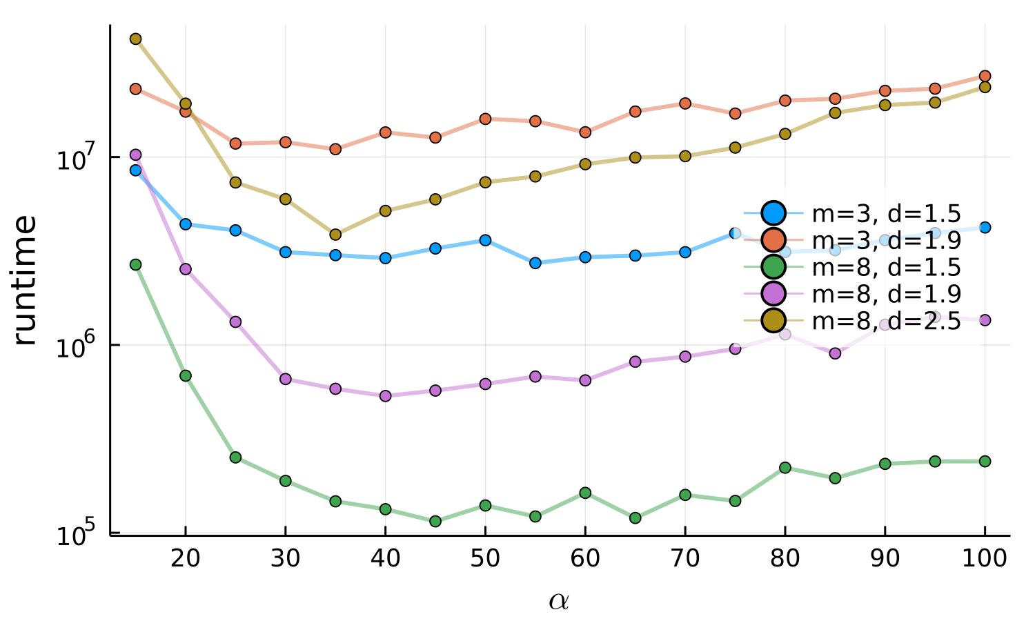
Figure 5. Average number (over 100 runs) of iterations Metropolis with different cooling parameters $\alpha$ took to optimize $\textsc{Cliff}_{d,m}$ functions of size $n=100$ with different settings of $d$ and $m$.

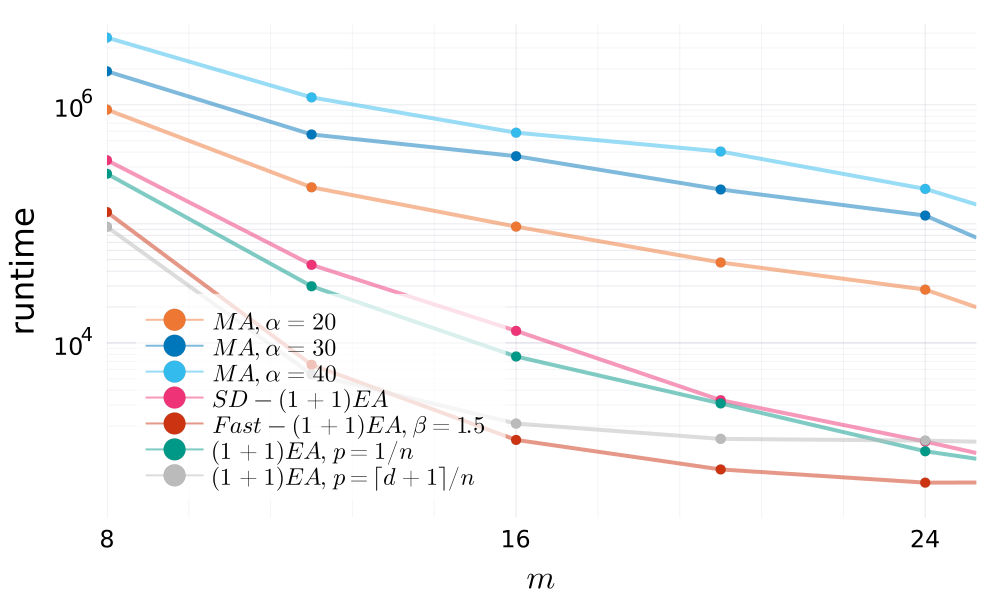
Figure 6. Comparison of MA with ${(1+1)}$ EA and its variants on $\textsc{Cliff}_{m,d}$ for $n=50$, $d=3$ and $m\in\{8,12,\dots,32\}$; averaged over 50 runs.

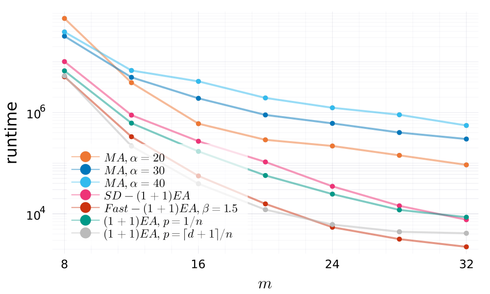
Figure 7. Comparison of MA with ${(1+1)}$ EA and its variants on $\textsc{Cliff}_{m,d}$ for $n=100$, $d=3$ and $m\in\{8,12,\dots,32\}$; averaged over 50 runs.

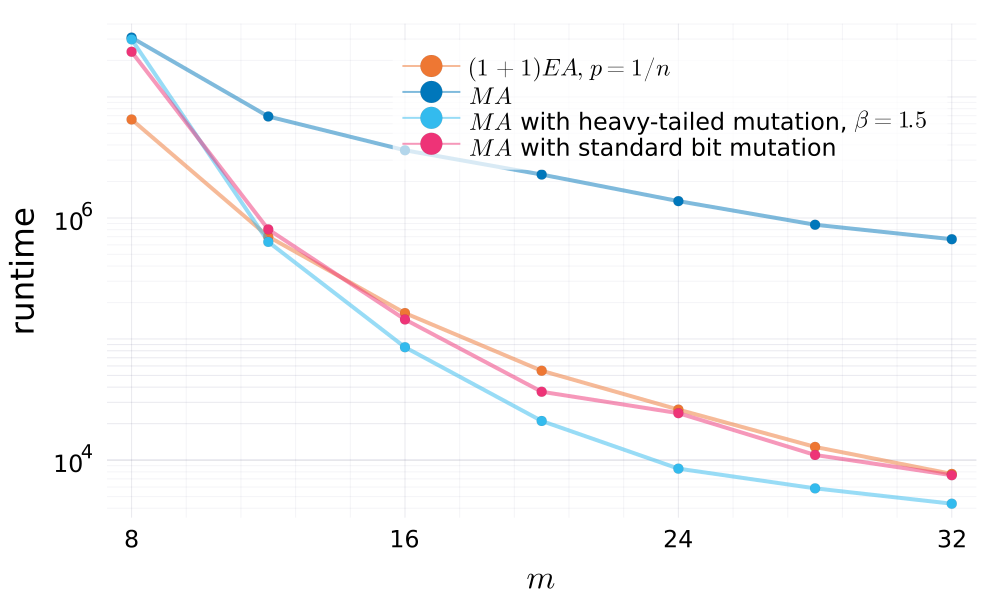
Figure 8. Comparison of ${(1+1)}$ EA and different variants of MA, including global mutation, on $\textsc{Cliff}_{m,d}$ for $n=100$, $\alpha=40$, $d=3$ and $m\in\{8,12,\dots,32\}$; averaged over 50 runs.

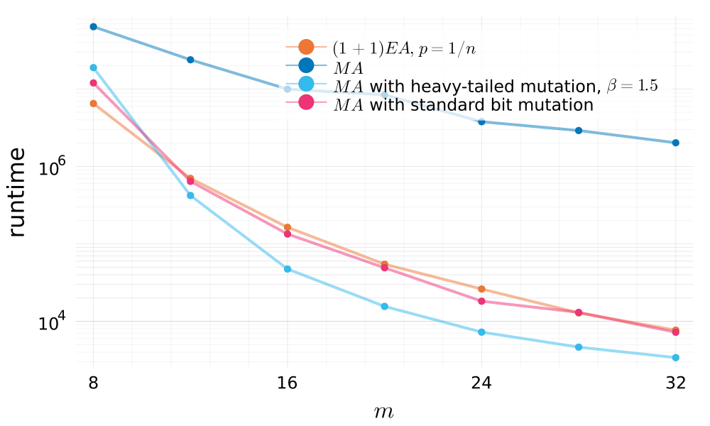
Figure 9. Comparison of ${(1+1)}$ EA and different variants of MA, including global mutation, on $\textsc{Cliff}_{m,d}$ for $n=100$, $\alpha=60$, $d=3$ and $m\in\{8,12,\dots,32\}$; averaged over 50 runs.

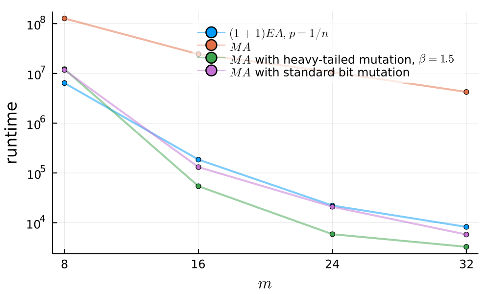
Figure 10. Comparison of ${(1+1)}$ EA and different variants of MA, including global mutation, on $\textsc{Cliff}_{m,d}$ for $n=100$, $\alpha=80$, $d=3$ and $m\in\{8,16,24,32\}$; averaged over 50 runs.