Mathematical theory for the interface mode in a waveguide bifurcated from a Dirac point

Abstract

In this paper, we prove the existence of a bound state in a waveguide that consists of two semi-infinite periodic structures separated by an interface. The two periodic structures are perturbed from the same periodic medium with a Dirac point and they possess a common band gap enclosing the Dirac point. The bound state, which is called interface mode here, decays exponentially away from the interface with a frequency located in the common band gap and can be viewed as a bifurcation from the Dirac point. Using the layer potential technique and asymptotic analysis, we first characterize the band gap opening for the two perturbed periodic media and derive the asymptotics of the Bloch modes near the band gap edges. By formulating the eigenvalue problem for the waveguide with two semi-infinite structures using a boundary integral equation over the interface and analyzing the characteristic values of the associated boundary integral operator, we prove the existence of the interface mode for the waveguide when the perturbation of the periodic medium is small.

1 Introduction

1.1 Background

The localization of acoustic and electromagnetic waves allows for the confinement of waves in a small volume or guiding the waves along the desired direction, and therefore has significant applications in the design of novel acoustic and optical devices [30, 31, 33, 34]. Several strategies have been proposed to achieve wave localization in different settings. For instance, a periodic medium with a single defect by changing the medium in a finite region can induce the so-called defect modes that are localized near the defect region. Such perturbations do not change the essential spectrum of the underlying differential operators but create isolated eigenvalues of finite multiplicity in a band gap of the periodic medium, with the eigenmodes decaying exponentially [3, 6, 19, 20]. Typically, the perturbations in such settings need to be large to create the defect modes [21, 26, 23]. Another way to create wave localization is by perturbing the periodic medium randomly in the whole domain. It can be shown that localized wave modes arise in the band gaps of the periodic medium, which is known as the Anderson localization [16, 17, 18, 33].

In this paper, we explore the idea of creating wave localization in a waveguide by perturbing a periodic structure differently along the positive and negative parts of the waveguide axis. In particular, we prove the existence of a localized wave mode (called bound state or interface mode) for such a configuration near the Dirac point of the periodic medium, which is a special vertex in the spectral band structure when two dispersion curves (surfaces) intersect in a linear (conic) manner. The investigation of Dirac points has attracted intense research efforts in recent years due to their important role in topological insulators. For example, Dirac points have been shown to occur in photonic graphene [1, 14] and photonic/phononic models with honeycomb lattices [4, 7, 28]. In general, topological phase transition takes place at a Dirac point. As such, near a Dirac point, eigenmodes localized around an interface can be generated by applying proper perturbations to the periodic operator on both sides of the interface. The bifurcation of eigenvalues from Dirac points was rigorously analyzed for one-dimensional Schrödinger operators [13], two-dimensional Schrödinger operators [15, 12, 10], and two-dimensional elliptic operators with smooth coefficients [27], all of which use domain wall models such that two periodic materials are “connected” adiabatically over a length scale that is much larger than the period of the structure. Note that such an adiabatic domain wall model may not be realistic for photonic/phononic materials with a sharp interface. In this work, we investigate the model when two different periodic media are glued directly such that the medium coefficient attains a jump across the interface. Our goal is to prove the existence of an interface mode near a Dirac point in the context of a waveguide, for which the interface between two periodic media is located at the origin of the waveguide axis. Such an interface mode is bifurcated from the Dirac point, and the corresponding eigenfrequency is located in the common band gap of the two periodic media enclosing the Dirac point. Furthermore, we prove that the eigenspaces at the band edges are swapped for the two periodic media, which demonstrates the topological phase transition of the medium at the Dirac point.

We point out that a bound state/interface mode arising from the bifurcation of a Dirac point in a one-dimensional system has been investigated under several different configurations. The existence and stability of interface mode eigenvalues were established by the transfer matrix method and the oscillatory theory for Sturm-Liouville operators in [29]. In another work, [35], the bulk-interface correspondence for 1D topological materials with inversion symmetry was established. Defect modes for 1D dislocated periodic media were studied in [11] and it was shown that the defect modes arise as bifurcations from the Dirac operator eigenmodes. Finally, the existence of a stable interface mode in a finite chain of high contrast bubbles that consists of two chains of different topological properties was reported numerically [2]. However, the analytical techniques in [11, 29, 35] only apply particularly to the 1D problems.

In this paper, we develop a new approach based on layer potential techniques and asymptotic analysis to investigate the existence of in-gap bound states for the waveguide. The approach overcomes the difficulty of discontinuous coefficients for the inhomogeneous medium in the waveguide and addresses the challenges brought by the presence of the sharp interface separating two different periodic media. The mathematical framework can be applied to study interface or edge modes in other photonic/phononic systems, which will be reported elsewhere. We refer [5] for a systematic review of the application of layer potential technique to various wave propagation problems in photonic/phononic materials consisting of subwavelength resonators.

1.2 Statement of main results

We start with the periodic waveguide in Figure 1 that attains a Dirac point in its band structure. Let $\Gamma_{-}=\mathbf{R}\times\{0\}$ and $\Gamma_{+}=\mathbf{R}\times\{\frac{1}{2}\}$ be two parallel walls of the waveguide in the plane $\mathbf{R}^{2}$, and let $\Gamma=\{0\}\times(0,\frac{1}{2})$. Denote $\mathbb{Z}^{*}:=\mathbb{Z}\backslash\{0\}$. Here $0$ is excluded from the index set in order to simplify the notation in the sequel. An array of identical obstacles $\{D_{n}\}_{n\in\mathbb{Z}^{*}}$ are arranged periodically in the center of the waveguide along the $x_{1}$-direction with period $1/2$. Here $D_{n}=z_{n}+D$ with $z_{n}=(\frac{2|n|-1}{4}\text{sgn}(n),\frac{1}{4})$ for $n\in\mathbb{Z}^{*}$ and $D$ is an open set centered at the origin. The domain outside the obstacles is denoted by $\Omega:=\mathbf{R}\times(0,\frac{1}{2})\backslash\cup_{n\in\mathbb{Z}^{*}}\overline{D_{n}}$. We consider a time-harmonic scalar wave that propagates in the waveguide at frequency $\omega$. The wave field $v$ satisfies the following Helmholtz equation

$$\Delta v(x)+\omega^{2}v(x)=0\quad\mbox{for}\;x\in\Omega.$$ (1.1)

We impose the following Neumann boundary condition on the waveguide walls

$$\frac{\partial v(x)}{\partial x_{2}}=0\quad\mbox{for}\;x\in\Gamma_{-}\bigcup\Gamma_{+},$$ (1.2)

and the Dirichlet boundary condition on the boundaries of the obstacles

$$v(x)=0\quad\mbox{for}\;x\in\cup_{n\in\mathbb{Z}^{*}}\partial D_{n}.$$ (1.3)

We point out that the above assumptions on the boundary conditions are not essential. The method developed in the paper applies to other boundary conditions; for instance, the Neumann boundary condition can be imposed over the obstacle boundaries.

Figure 1: The waveguide with periodically arranged obstacles.

We shall make the following assumptions on the spectrum of the operator $-\Delta$ for the above period-$1/2$ structure $\Omega$. The reader is referred to Section 2.1 for terminologies arising from the Floquet-Bloch theory.

Assumption 1.1.

1. The first spectral band $(p,\mu_{1}(p))$ of the period-$1/2$ structure $\Omega$ is smooth for $p\in[-2\pi,2\pi]$, and can be extended analytically in a complex neighborhood of $\mathbf{R}$. Moreover, the eigenspace corresponding to the first spectral band is one dimensional and is given by $\text{span}\{v_{1}(\cdot;p)\}$. The analytic continuation of $v_{1}(\cdot;p)$ from $\mathbf{R}$ to its complex neighborhood also holds.

2. The slope of $\mu_{1}(\cdot)$ at $p=\pi$ satisfies $\mu_{1}^{\prime}(\pi)=\alpha_{*}>0$.

3. $\lambda_{*}:=\mu_{1}(\pi)$ is not in the point spectrum of the period-$1/2$ structure.

4. $\mu_{1}(p)\neq\lambda_{*}$ for $p\neq\pi$, and consequently $\lambda_{*}=\max_{0\leq p\leq\pi}\mu_{1}(p)=\min_{\pi\leq p\leq 2\pi}\mu_{1}(p)$. In addition, the maximum of the first spectral band is smaller than or equal to the minimum of the second spectral band.

Remark 1.2.

All the statements in Assumption 1.1 can be proved rigorously in the case when the size of the particle $D$ is sufficiently small by using asymptotic analysis.

Remark 1.3.

It is generally believed that the point spectrum is empty for a periodic structure shown in Figure 1. However, as pointed out in [25], its rigorous proof is an open question.

Remark 1.4.

The statement (4) in Assumption 1.1 is similar to the spectral no-fold assumption in [15] (cf. Definition 7.1). We conjecture that it is not essential for the main result Theorem 1.11 to hold. This issue shall be investigated in a separate paper.

In the sequel, we shall treat the above period-1/2 structure $\Omega$ as a period-1 structure whose primitive cell is given by $Y=(0,1)\times(0,\frac{1}{2})$ and the associated Brillouin zone is $[0,2\pi]$. For the period-1 structure, each period consists of two obstacles. We denote by $(\lambda_{n}(p),u_{n}(\cdot;p))$ ($n\geq 1$) the eigenpairs for the $n$-th spectral band. Note that the spectral band structure of the period-1 structure can be obtained by ‘folding’ the bands of the period-1/2 structure. This allows for the creation of a Dirac point $(p_{*}=\pi,\lambda_{*})$ in the spectrum of the period-1 structure in the Brillouin zone as stated in the following proposition.

Proposition 1.5.

A linear band crossing occurs at $\left(p_{*},\lambda_{*}\right)$ between the first and second dispersion curves of the period-1 structure $\Omega$ with the following properties:

1. $\lambda_{*}=\lambda_{1}(p_{*})=\lambda_{2}(p_{*})$, and $\lambda_{*}$ is an eigenvalue of multiplicity 2.

2. Denote by $\mu_{2}(p):=\mu_{1}(2\pi-p)$ and $v_{2}(\cdot;p):=\overline{v_{1}(\cdot;2\pi-p)}$, then the first and second spectral bands and the corresponding eigenfunctions can be chosen as below:

   $$\lambda_{1}(p)=\left\{\begin{aligned} &\mu_{1}(p),\quad p\in[0,\pi),\\ &\mu_{2}(p),\quad p\in[\pi,2\pi],\end{aligned}\right.\quad u_{1}(\cdot,p)=\left\{\begin{aligned} &v_{1}(\cdot;p),\quad p\in[0,\pi),\\ &v_{2}(\cdot;p),\quad p\in[\pi,2\pi],\end{aligned}\right.$$

   and

   $$\lambda_{2}(p)=\left\{\begin{aligned} &\mu_{2}(p),\quad p\in[0,\pi),\\ &\mu_{1}(p),\quad p\in[\pi,2\pi],\end{aligned}\right.\quad u_{2}(\cdot,p)=\left\{\begin{aligned} &v_{2}(\cdot;p),\quad p\in[0,\pi),\\ &v_{1}(\cdot;p),\quad p\in[\pi,2\pi].\end{aligned}\right.$$

Remark 1.6.

The function $v_{1}(\cdot;p)$ above stands for the Bloch eigenmode when the primitive cell is $(0,\frac{1}{2})\times(0,\frac{1}{2})$. Specifically, $v_{1}(\cdot;p)$ satisfies the quasi-periodic boundary condition $v_{1}(x_{1}+\frac{1}{2},x_{2};p)=e^{i\frac{p}{2}}v_{1}(x_{1},x_{2};p)$.

We assume that the periodic structure $\Omega$ attains reflection symmetry, which is a consequence of the following assumption.

Assumption 1.7.

The obstacle $D$ attains the reflection symmetry such that its boundary $\partial D$ is parameterized by $\left\{(\theta,r(\theta)):0\leq\theta\leq 2\pi\right\}$ in the polar coordinate, in which $r(\theta)=r(\pi-\theta)$ for $0\leq\theta\leq\pi$.

We have the following corollary for the eigenmodes at the Dirac point $(p_{*},\lambda_{*})$.

Corollary 1.8.

Under Assumptions 1.1 and 1.7, the eigenmodes at the Dirac point $(p_{*},\lambda_{*})$ can be chosen to be odd and even functions with respect to $x_{1}$. More precisely, $\text{span}\{u_{1}(\cdot;\pi),u_{2}(\cdot;\pi)\}=\text{span}\{\phi_{1},\phi_{2}\}$ with

$$\phi_{1}(-x_{1},x_{2})=-\phi_{1}(x_{1},x_{2}),\quad\phi_{2}(-x_{1},x_{2})=\phi_{2}(x_{1},x_{2}).$$

Let

$$\bm{\varphi}_{1}(x) =\left(\partial_{n}\phi_{1}|_{\partial D_{1}}(x+z_{1}),\partial_{n}\phi_{1}|_{\partial D_{2}}(x+z_{2})\right)^{T}\in(H^{-\frac{1}{2}}(\partial D))^{2},$$ (1.4)

$$\bm{\varphi}_{2}(x) =\left(\partial_{n}\phi_{2}|_{\partial D_{1}}(x+z_{1}),\partial_{n}\phi_{2}|_{\partial D_{2}}(x+z_{2})\right)^{T}\in(H^{-\frac{1}{2}}(\partial D))^{2},$$ (1.5)

then

$$\bm{\varphi}_{1}=(\varphi_{ref},\varphi),\quad\bm{\varphi}_{2}=(\varphi,-\varphi_{ref}),$$

for some real-valued function $\varphi\in H^{-\frac{1}{2}}(\partial D)$ and $\varphi_{ref}(x_{1},x_{2}):=\varphi(-x_{1},x_{2}).$

Proof.

See Appendix A. ∎

For ease of notation, we denote $v_{i}=v_{i}(\cdot,\pi)$ for $i=1,2$.

Remark 1.9.

The eigenmodes $\phi_{1},\phi_{2}$ introduced in the above lemma are linear combinations of $v_{1}$ and $v_{2}$. We note that $\phi_{1}|_{\Gamma}$ vanishes due to the odd parity. Thus both $v_{1}|_{\Gamma}$ and $v_{2}|_{\Gamma}$ are proportional to $\phi_{2}|_{\Gamma}$. This relationship will be used later.

Figure 2: Waveguide with perturbations: (a) The distance between each pair of two obstacles in one periodic cell is $\frac{1}{2}-2\delta$; (b) The distance between each pair of two obstacles in one periodic cell is $\frac{1}{2}+2\delta$; (c) The waveguide obtained by gluing the structures in (a) and (b) along the interface $\Gamma$.

For technical reasons, we make the following assumption which guarantees the analyticity of the Green’s function for the empty waveguide, and will be used in the proof of Proposition 3.5.

Assumption 1.10.

The Dirac energy level $\lambda_{*}$ is away from the singular frequencies such that $\lambda_{*}\neq(2m+1)\pi$ for $m\in\mathbb{N}$.

We now introduce perturbations to the periodic structure along the negative and positive parts of the waveguide axis. Let $0<\delta\ll 1$. The obstacle $D_{n}$ is translated to $\tilde{D}_{n,\delta}$ ($n\in\mathbb{Z}^{*}$) with the mass center given by

$$\tilde{z}_{n,\delta}=\left\{\begin{aligned} &z_{n}+\delta\bm{e}_{1},\quad\text{n is even},\\ &z_{n}-\delta\bm{e}_{1},\quad\text{n is odd}.\end{aligned}\right.$$

The corresponding structure is depicted in Figure 2(c), which can be viewed as a joint structure that glues the two semi-infinite periodic structures in Figure 2(a) and 2(b) along the interface $\Gamma$. Define $\tilde{\Omega}_{\delta}:=\mathbf{R}\times(0,\frac{1}{2})\backslash\bigcup_{n}\overline{\tilde{D}_{n,\delta}}$. An interface mode $u$ for the waveguide in Figure 2(c) is a finite-energy solution to the following spectral problem:

$$\left\{\begin{aligned} &(\Delta_{x}+\lambda)u(x;\lambda)=0,\quad x\in\tilde{\Omega}_{\delta},\\ &u(x;\lambda)=0,\quad x\in\cup_{n\in\mathbb{Z}^{*}}\partial\tilde{D}_{n,\delta},\\ &\frac{\partial}{\partial x_{2}}u(x;\lambda)=0,\quad x\in\Gamma_{-}\bigcup\Gamma_{+}.\end{aligned}\right.$$ (1.6)

We define the Sobolev space

$$H_{b}^{1}(\tilde{\Omega}_{\delta};\Delta):=\left\{u\in H^{1}(\tilde{\Omega}_{\delta}):\Delta u\in L^{2}(\tilde{\Omega}_{\delta}),\frac{\partial u}{\partial x_{2}}|_{\Gamma_{-}\bigcup\Gamma_{+}}=0,u|_{\partial\tilde{D}_{n,\delta}}=0,n\in\mathbb{Z}^{*}\right\}.$$

Then an interface mode corresponds to an eigenfunction of the operator

$$\tilde{\mathcal{L}}_{\delta}:H_{b}^{1}(\tilde{\Omega}_{\delta};\Delta)\subset L^{2}(\tilde{\Omega}_{\delta})\to L^{2}(\tilde{\Omega}_{\delta}),\quad\phi\mapsto-\Delta\phi.$$

Now we can state the main result of the paper as follows:

Theorem 1.11.

Under the Assumptions 1.1, 1.7 and 1.10, if $t_{*}$ defined in (3.15) is nonzero, then there exists $\delta_{0}>0$ such that for $|\delta|<\delta_{0}$, the spectral problem (1.6) attains an eigenpair $(u^{\star},\lambda^{\star})\in L^{2}(\tilde{\Omega}_{\delta})\times\mathbf{R}$ for $\lambda^{\star}$ near $\lambda_{*}$. Moreover,

$$\sigma_{p}(\tilde{\mathcal{L}}_{\delta})\bigcap\left(\lambda_{*}-\big{|}\frac{t_{*}}{\gamma_{*}}\big{|}\delta,\lambda_{*}+\big{|}\frac{t_{*}}{\gamma_{*}}\big{|}\delta\right)=\{\lambda^{\star}\},$$

where $\gamma_{*}$ and $t_{*}$ are defined in (3.14). In addition, $u^{\star}$ decays exponentially away from the interface $\Gamma$ as $|x_{1}|\to\infty$.

Remark 1.12.

The assumption $t_{*}\neq 0$ guarantees that the perturbed structures in Figure 2(a) and 2(b) has a common band gap near the Dirac point $(p_{*},\lambda_{*})$ of the unperturbed structure; See Corollary 3.9. This assumption can be verified when the size of the obstacles is sufficiently small by using asymptotic analysis.

1.3 Outline

The rest of the paper is organized as follows. In Section 2, we briefly review the Floquet-Bloch theory for periodic differential operators and introduce the Green’s functions for periodic waveguide structures. We also recall the Gohberg-Sigal theory which shall be used in the investigation of the spectral problem (1.6). In Section 3, we present the asymptotic expansions of Bloch eigenvalues and eigenfunctions near the Dirac point $(p_{*},\lambda_{*})$ for the periodic structures in Figure 2(a)(b). In particular, we prove that a band gap is opened near the Dirac point after the perturbation. Furthermore, the eigenspaces at the band edges are swapped for these two periodic structures. These results are presented in Theorem 3.6 and Corollary 3.9. Finally, in Section 4, we reformulate the spectral problem (1.6) by using a boundary integral equation and prove Theorem 1.11 by analyzing the characteristic values of the associated boundary integral operator.

2 Preliminaries

2.1 Floquet-Bloch theory for periodic structures

For clarity, we focus on the periodic waveguide structure in Figure 1. Let $\mathcal{L}:H_{b}^{1}(\Omega;\Delta)\subset L^{2}(\Omega)\to L^{2}(\Omega)$ be the Laplacian operator. The eigenvalue problem for the waveguide is to solve for all eigenpairs that satisfy the following equations

$$\left\{\begin{aligned} &(\mathcal{L}-\lambda)u(x;\lambda)=0,\quad x\in\Omega,\\ &u(x;\lambda)=0,\quad x\in\cup_{n\in\mathbb{Z}^{*}}\partial D_{n},\\ &\frac{\partial}{\partial x_{2}}u(x;\lambda)=0,\quad x\in\Gamma_{-}\bigcup\Gamma_{+}.\end{aligned}\right.$$ (2.1)

To study the spectrum $\sigma(\mathcal{L})$ of $\mathcal{L}$, we consider a family of operators $\mathcal{L}(p)$, where $p$ lies in the Brillouin zone $B:=[0,2\pi]$. More precisely, $\mathcal{L}(p)$ is the Laplacian operator restricted to the function space with the quasi-periodic boundary condition:

$$\mathcal{L}(p):H_{p,b}^{1}(\Omega;\Delta)\subset L^{2}_{loc}(\Omega)\to L^{2}_{loc}(\Omega),\quad\phi\to-\Delta\phi.$$

In the above,

$$H_{p,b}^{1}(\Omega;\Delta):=\Big{\{}u\in H_{loc}^{1}(\Omega): \Delta u\in L^{2}_{loc}(Y),\frac{\partial u}{\partial x_{2}}|_{\Gamma_{-}\bigcup\Gamma_{+}}=0,u|_{\partial D_{n}}=0,n\in\mathbb{Z}^{*},$$

$$u(x+\bm{e}_{1})=e^{ip}u(x),\frac{\partial u}{\partial x_{1}}(x+\bm{e}_{1})=e^{ip}\frac{\partial u}{\partial x_{1}}(x)\Big{\}}.$$

For each $p\in B$, the spectral theory for self-adjoint operators (cf. [9, 32]) states that $\sigma(\mathcal{L}(p))$ consists of a discrete set of real eigenvalues

$$0<\lambda_{1}(p)\leq\lambda_{2}(p)\leq\cdots\leq\lambda_{n}(p)\leq\cdots.$$

We denote by $u_{n}(x;p)$ the eigenfunction associated with the eigenvalue $\lambda_{n}(p)$, which is also called the $n$-th Bloch mode at quasi-momentum $p$. We have the following standard results for the dispersion relation $\lambda_{n}(p)$ (cf. [25]):

Proposition 2.1.

(1) $\lambda_{n}(p)$ ($n\geq 1$) is Lipschitz continuous with respect to $p\in B$;
(2) $\lambda_{n}(p)$ ($n\geq 1$) can be periodically extended to $p\in\mathbf{R}$ with period $2\pi$, i.e. $\lambda_{n}(p+2\pi)=\lambda_{j}(p)$. Moreover, $\lambda_{n}(p)=\lambda_{j}(-p)$.

For each integer $n$, let

$$\lambda_{n}^{-}=\min_{p\in\mathcal{B}}\lambda_{n}(p),\quad\lambda_{n}^{+}=\max_{p\in\mathcal{B}}\lambda_{n}(p).$$

The Floquet-Bloch theory states that the spectrum $\sigma(\mathcal{L})$ is given by

$$\sigma(\mathcal{L})=\bigcup_{p\in\mathcal{B}}\sigma(\mathcal{L}(p))=\bigcup_{n\geq 1}I_{n},\quad I_{n}:=\left[\lambda_{n}^{-},\lambda_{n}^{+}\right].$$

We say that a band gap opens between the $n$-th and $n+1$-th band if $\lambda_{n}^{+}<\lambda_{n+1}^{-}$; See Figure 3 for an example.

Figure 3: An example of the band structure: the first four bands of the spectrum are depicted in the figure. Note that there is a spectral gap between the second and third bands.

2.2 The Green’s function and representation of solutions for the periodic structure

We present some properties of the Green’s function $G(x,y,\lambda)$ for the waveguide problem (2.1) at $\lambda=\lambda_{*}$, which is defined to be the unique physical solution to the following equations:

$$\left\{\begin{aligned} &(\Delta_{x}+\lambda)G(x,y;\lambda_{*})=\tilde{\delta}(x-y),\quad x,y\in\Omega,\\ &G_{\delta}(x,y;\lambda_{*})=0,\quad x\in\cup_{n\in\mathbb{Z}^{*}}\partial D_{n},\\ &\frac{\partial}{\partial x_{2}}G(x,y;\lambda_{*})=0,\quad x\in\Gamma_{-}\bigcup\Gamma_{+}.\end{aligned}\right.$$

Here $\tilde{\delta}(\cdot)$ denotes the Dirac delta function. We follow closely the discussions in [22]. The existence and uniqueness of the Green’s function can be established by using the limiting absorbing principle, which gives rise to a physical solution to the wave propagation problem (2.1) as the limit of the unique finite-energy solution of the corresponding model with absorption when the absorption tends to zero. More precisely, the Green’s function for the waveguide problem (2.1) can be defined as the limit of the Green’s function $G(x,y;\lambda+i\varepsilon)$ for the waveguide problem (2.1) with $\lambda$ being replaced by $\lambda+i\varepsilon$ as $\varepsilon\to 0$.

We apply the Floquet-Bloch theory to derive the asymptotic behavior of $G(x,y,\lambda_{*})$ at infinity. Recall that $(\lambda_{n}(p),u_{n}(x;p)),n\geq 1$ are the Bloch eigenpairs associated with the periodic structure. First, by using the Floquet transform, the following spectral representation of the Green’s function holds:

$$G(x,y;\lambda_{*})=\lim_{\varepsilon\to 0^{+}}G(x,y;\lambda_{*}+i\varepsilon) =\displaystyle{\frac{1}{2\pi}\lim_{\varepsilon\to 0^{+}}\int_{0}^{2\pi}\frac{u_{1}(x;p)\overline{u_{1}(y;p)}}{\lambda_{*}-\lambda_{1}(p)+i\varepsilon}dp+\frac{1}{2\pi}\lim_{\varepsilon\to 0^{+}}\int_{0}^{2\pi}\frac{u_{2}(x;p)\overline{u_{2}(y;p)}}{\lambda_{*}-\lambda_{2}(p)+i\varepsilon}dp}$$

$$+\displaystyle{\frac{1}{2\pi}\int_{0}^{2\pi}\sum_{n=3}^{+\infty}\frac{u_{n}(x;p)\overline{u_{n}(y;p)}}{\lambda_{*}-\lambda_{n}(p)}dp.}$$

Note that by Proposition 1.5, there holds

$$\int_{0}^{2\pi}\frac{u_{1}(x;p)\overline{u_{1}(y;p)}}{\lambda_{*}-\lambda_{1}(p)+i\varepsilon}dp+\int_{0}^{2\pi}\frac{u_{2}(x;p)\overline{u_{2}(y;p)}}{\lambda_{*}-\lambda_{2}(p)+i\varepsilon}dp=\int_{0}^{2\pi}\frac{v_{1}(x;p)\overline{v_{1}(y;p)}}{\lambda_{*}-\mu_{1}(p)+i\varepsilon}dp+\int_{0}^{2\pi}\frac{v_{2}(x;p)\overline{v_{2}(y;p)}}{\lambda_{*}-\mu_{2}(p)+i\varepsilon}dp.$$

Taking the limit as $\varepsilon\to 0$ yields (see Remark 8 in [22]):

$$G(x,y;\lambda_{*})= -\frac{i}{2}\frac{v_{1}(x)\overline{v_{1}(y)}}{\alpha_{*}}+\frac{1}{2\pi}p.v.\int_{0}^{2\pi}\frac{v_{1}(x;p)\overline{v_{1}(y;p)}}{\lambda_{*}-\mu_{1}(p)}dp$$ (2.2)

$$-\frac{i}{2}\frac{v_{2}(x)\overline{v_{2}(y)}}{\alpha_{*}}+\frac{1}{2\pi}p.v.\int_{0}^{2\pi}\frac{v_{2}(x;p)\overline{v_{2}(y;p)}}{\lambda_{*}-\mu_{2}(p)}dp$$

$$+\frac{1}{2\pi}\int_{0}^{2\pi}\sum_{n\geq 3}\frac{u_{n}(x;p)\overline{u_{n}(y;p)}}{\lambda_{*}-\lambda_{n}(p)}dp.$$

Moreover, it can be shown that $G$ admits the following decomposition for fixed $y$ (see Remark 9 in [22]):

$$G(x,y;\lambda_{*})=G_{0}^{+}(x,y;\lambda_{*})-i\frac{v_{1}(x)\overline{v_{1}(y)}}{\alpha_{*}},\quad x_{1}\to\infty,$$ (2.3)

and

$$G(x,y;\lambda_{*})=G_{0}^{-}(x,y;\lambda_{*})-i\frac{v_{2}(x)\overline{v_{2}(y)}}{\alpha_{*}},\quad x_{1}\to-\infty.$$ (2.4)

where $G_{0}^{+}(x,y;\lambda)$ ($G_{0}^{-}(x,y;\lambda)$) decays exponentially as $x_{1}\to+\infty$ ($x_{1}\to-\infty$). We remark that (2.3)-(2.4) define the so-called radiation condition for the Green’s function $G$, with $v_{1}$ and $v_{2}$ being the right and left propagating modes respectively.

We present some properties for $v_{1}$ and $v_{2}$ in the next two lemmas.

Lemma 2.2.

There exists some $\tau\in\mathbb{C}$ s.t. $|\tau|=1$ and

$$v_{2}(x_{1},x_{2})=\tau v_{1}(-x_{1},x_{2}).$$

Proof.

With Remark 1.6 and Assumption 1.7, it is straightforward to check that $v_{1}(-x_{1},x_{2})$ is also a Bloch mode with the same quasi-periodic boundary condition as $v_{2}$. Then the proof is completed by recalling that the dimension of the eigenspace is one as stated in Assumption 1.1. ∎

Let

$$\mathcal{V}(\lambda):=\big{\{}u\in H^{1}_{loc}(\Omega):(\Delta+\lambda)u(x)=0\enspace\mbox{in}\;\Omega,\frac{\partial u}{\partial x_{2}}\big{|}_{\Gamma_{-}\bigcup\Gamma_{+}}=0,u\big{|}_{\partial D_{n}}=0,n\in\mathbb{Z}^{*}\big{\}}.$$

Then $v_{1},v_{2}\in\mathcal{V}(\lambda_{*})$. Moreover, we have the following proposition.

Lemma 2.3.

The right- and left-propagating modes $v_{1}$ and $v_{2}$ satisfy

$$\int_{\Gamma}\frac{\partial v_{1}}{\partial x_{1}}\overline{v_{1}}dx_{2}=\frac{i}{2}\mu_{1}^{\prime}(\pi)=\frac{i}{2}\alpha_{*},\quad\int_{\Gamma}\frac{\partial v_{2}}{\partial x_{1}}\overline{v_{2}}dx_{2}=-\frac{i}{2}\alpha_{*}.$$ (2.5)

Moreover, for each $u\in\mathcal{V}(\lambda_{*})$ that decays exponentially as $x_{1}\to\infty$, there holds

$$\int_{\Gamma}\frac{\partial v_{1}}{\partial x_{1}}\overline{u}dx_{2}=\int_{\Gamma}\frac{\partial\overline{u}}{\partial x_{1}}v_{1}dx_{2}=\int_{\Gamma}\frac{\partial v_{2}}{\partial x_{1}}\overline{u}dx_{2}=\int_{\Gamma}\frac{\partial\overline{u}}{\partial x_{1}}v_{2}dx_{2}=0.$$ (2.6)

Proof.

We consider the following sesquilinear form defined on $\mathcal{V}(\lambda)$:

$$q(v,w;x)=\int_{\Gamma_{x}}\big{(}\frac{\partial v}{\partial x_{1}}\overline{w}-\frac{\partial\overline{w}}{\partial x_{1}}v\big{)}dx_{2},\quad\Gamma_{x}:=\{x_{2}:(x,x_{2})\in\Omega\},\quad v,w\in\mathcal{V}(\lambda).$$

It is shown in [22] that $q(v,w;x)$ is independent of $x\in\mathbf{R}$, and moreover,

$$q(v_{n},v_{m})=i\mu_{n}^{\prime}(\pi)\delta_{nm},\quad n,m=1,2.$$

Using Lemma 2.2, we have

$$0=q(v_{2},v_{1})=\int_{\Gamma}\big{(}\frac{\partial v_{2}}{\partial x_{1}}\overline{v_{1}}-\frac{\partial\overline{v_{1}}}{\partial x_{1}}v_{2}\big{)}dx_{2}=-\tau\int_{\Gamma}\big{(}\frac{\partial v_{1}}{\partial x_{1}}\overline{v_{1}}+\frac{\partial\overline{v_{1}}}{\partial x_{1}}v_{1}\big{)}dx_{2}.$$

This, combined with the equality $q(v_{1},v_{1})=i\mu_{1}^{\prime}(\pi)$ for $n=1,2$, yield $\int_{\Gamma}\frac{\partial v_{1}}{\partial x_{1}}\overline{v_{1}}dx_{2}=\frac{i}{2}\mu_{1}^{\prime}(\pi)$. Similarly, we have $\int_{\Gamma}\frac{\partial v_{2}}{\partial x_{1}}\overline{v_{2}}dx_{2}=-\frac{i}{2}\alpha_{*}$. Next, since $q(v_{i},u;x)$ ($i=1,2$) is independent of $x$, we have for positive integer $N$,

$$\int_{\Gamma}\big{(}\frac{\partial v_{1}}{\partial x_{1}}\overline{u}-\frac{\partial\overline{u}}{\partial x_{1}}v_{1}\big{)}dx_{2}=q(v_{1},u)=\int_{\Gamma_{N}}\big{(}\frac{\partial v_{1}}{\partial x_{1}}\overline{u}-\frac{\partial\overline{u}}{\partial x_{1}}v_{1}\big{)}dx_{2},$$

$$\int_{\Gamma}\big{(}\frac{\partial v_{1}}{\partial x_{1}}\overline{u}+\frac{\partial\overline{u}}{\partial x_{1}}v_{1}\big{)}dx_{2}=-\frac{1}{\tau}q(v_{2},u)=-\frac{1}{\tau}\int_{\Gamma_{N}}\big{(}\frac{\partial v_{2}}{\partial x_{1}}\overline{u}-\frac{\partial\overline{u}}{\partial x_{1}}v_{2}\big{)}dx_{2}.$$

Since $u$ decays exponentially,

$$\int_{\Gamma}\big{(}\frac{\partial v_{1}}{\partial x_{1}}\overline{u}-\frac{\partial\overline{u}}{\partial x_{1}}v_{1}\big{)}dx_{2}=\lim_{N\to+\infty}\int_{\Gamma_{N}}\big{(}\frac{\partial v_{1}}{\partial x_{1}}\overline{u}-\frac{\partial\overline{u}}{\partial x_{1}}v_{1}\big{)}dx_{2}=0,$$

$$\int_{\Gamma}\big{(}\frac{\partial v_{1}}{\partial x_{1}}\overline{u}+\frac{\partial\overline{u}}{\partial x_{1}}v_{1}\big{)}dx_{2}=-\frac{1}{\tau}\lim_{N\to+\infty}\int_{\Gamma_{N}}\big{(}\frac{\partial v_{2}}{\partial x_{1}}\overline{u}-\frac{\partial\overline{u}}{\partial x_{1}}v_{2}\big{)}dx_{2}=0.$$

By adding those two identities together, we conclude that $\displaystyle{\int_{\Gamma}\frac{\partial v_{1}}{\partial x_{1}}\overline{u}dx_{2}=\int_{\Gamma}\frac{\partial\overline{u}}{\partial x_{1}}v_{1}dx_{2}=0}$. Following the same argument, $\displaystyle{\int_{\Gamma}\frac{\partial v_{2}}{\partial x_{1}}\overline{u}dx_{2}=\int_{\Gamma}\frac{\partial\overline{u}}{\partial x_{1}}v_{2}dx_{2}=0}$. ∎

We next present some useful properties of the Green’s function $G(x,y;\lambda_{*})$.

Lemma 2.4.

For $x,y\in\Omega$ and $x\neq y$, the Green function in (2.2) satisfies

$$G(x,y;\lambda_{*})=G(y,x;\lambda_{*}).$$ (2.7)

On the other hand, when $y\in\Gamma:=\{0\}\times(0,\frac{1}{2})$, there holds

$$G((x_{1},x_{2}),y;\lambda_{*})=G((-x_{1},x_{2}),y;\lambda_{*}),\quad\forall(x_{1},x_{2})\in\Omega.$$ (2.8)

Proof.

We only prove (2.7) and the proof of (2.8) follows similarly. For $x\neq y$, define $u(z):=G(z,x;\lambda_{*})$ and $w(z):=G(z,y;\lambda_{*})$. Let $\Omega_{-N,N}:=\Omega\bigcap\big{(}(-N,N)\times(0,\frac{1}{2})$) where $N$ is a positive integer. Then $x,y\in\Omega_{N}$ for sufficiently large $N$. An integration by part yields

$$w(x)-u(y) =\int_{\Omega_{-N,N}}(\Delta+\lambda_{*})u(z)w(z)-(\Delta+\lambda_{*})w(z)u(z)dz$$ (2.9)

$$=\int_{\Gamma_{N}}\left(\frac{\partial u}{\partial z_{1}}w-\frac{\partial w}{\partial z_{1}}u\right)dz_{2}-\int_{\Gamma_{-N}}\left(\frac{\partial u}{\partial z_{1}}w-\frac{\partial w}{\partial z_{1}}u\right)dz_{2}.$$

By (2.3) and Lemma 2.3, as $N\to+\infty$, we have

$$\lim_{N\to+\infty}\int_{\Gamma_{N}}\frac{\partial u}{\partial z_{1}}w-\frac{\partial w}{\partial z_{1}}udz_{2}=-\frac{1}{\alpha_{*}^{2}}\left(\overline{v_{1}(x)\cdot v_{1}(y)}\int_{\Gamma}\frac{\partial v_{1}}{\partial z_{1}}v_{1}dz_{2}-\overline{v_{1}(x)\cdot v_{1}(y)}\int_{\Gamma}\frac{\partial v_{1}}{\partial z_{1}}v_{1}dz_{2}\right)=0.$$

Similarly,

$$\lim_{N\to+\infty}\int_{\Gamma_{-N}}\frac{\partial u}{\partial z_{1}}w-\frac{\partial w}{\partial z_{1}}udz_{2}=-\frac{1}{\alpha_{*}^{2}}\left(\overline{v_{2}(x)\cdot v_{2}(y)}\int_{\Gamma}\frac{\partial v_{2}}{\partial z_{1}}v_{2}dz_{2}-\overline{v_{2}(x)\cdot v_{2}(y)}\int_{\Gamma}\frac{\partial v_{2}}{\partial z_{1}}v_{2}dz_{2}\right)=0.$$

Thus $w(x)=u(y)$, which implies $G(y,x;\lambda_{*})=G(x,y;\lambda_{*})$ from definition of $w$ and $u$. ∎

Finally, as an application of Green’s function, we present a representation formula for the solution to the Helmholtz equation in the semi-infinite structure $\Omega_{+}:=\{x=(x_{1},x_{2}):x\in\Omega,x_{1}>0\}$. Denote

$$\mathcal{V}^{+}(\lambda):=\big{\{}u\in H^{1}_{loc}(\Omega^{+}):(\Delta+\lambda)u(x)=0\;\mbox{in}\;\Omega^{+},\frac{\partial u}{\partial x_{2}}\big{|}_{\Gamma_{-}\bigcup\Gamma_{+}}=0,u\big{|}_{\partial D_{n}}=0,n\geq 1\big{\}}.$$

Proposition 2.5.

If $u\in\mathcal{V}^{+}(\lambda_{*})$ satisfies the right-going condition such that

$$u(x)=c_{1}v_{1}(x)+u^{+}_{0}(x)\text{ for some $c_{1}\in\mathbb{C}$ and $u^{+}_{0}(x)$ decays exponentially as $x_{1}\to+\infty$},$$

then

$$u(x)=2\int_{\Gamma}G(x,y;\lambda_{*})\frac{\partial u}{\partial x_{1}}(0^{+},y_{2})dy_{2},\quad x\in\Omega^{+}.$$ (2.10)

Proof.

Suppose $u\in\mathcal{V}^{+}(\lambda_{*})$. Define the following even extension of $u$:

$$\tilde{u}(x_{1},x_{2})=\left\{\begin{aligned} &u(x_{1},x_{2}),\quad x_{1}\geq 0,\\ &u(-x_{1},x_{2}),\quad x_{1}<0.\end{aligned}\right.$$ (2.11)

Let $\Omega_{x,y}:=\Omega\bigcap((x,y)\times(0,\frac{1}{2}))$. For $y=(y_{1},y_{2})\in\Omega^{+}$ and positve integer $N$, an integration by parts shows that

$$\tilde{u}(y) =\int_{\Omega_{0,N}}(\Delta_{x}+\lambda_{*})G(x,y;\lambda_{*})\tilde{u}(x)-(\Delta_{x}+\lambda_{*})\tilde{u}(x)G(x,y;\lambda_{*})dx$$

$$=\int_{\Gamma_{N}}\left(\frac{\partial}{\partial x_{1}}G(x,y;\lambda_{*})\tilde{u}(x)-\frac{\partial}{\partial x_{1}}\tilde{u}(x)G(x,y;\lambda_{*})\right)dx_{2}$$

$$\quad-\int_{\Gamma}\left(\frac{\partial}{\partial x_{1}}G(x,y;\lambda_{*})\tilde{u}(0^{+},x_{2})-\frac{\partial}{\partial x_{1}}\tilde{u}(0^{+},x_{2})G(x,y;\lambda_{*})\right)dx_{2},$$

where $\tilde{u}(0^{+},x_{2})=u(x)\big{|}_{\Gamma}$. By the right-going condition of $u(\cdot)$, we have

$$\lim_{N\to+\infty}\int_{\Gamma_{N}}\Big{(}\frac{\partial}{\partial x_{1}}G(x ,y;\lambda_{*})\tilde{u}(x)-\frac{\partial}{\partial x_{1}}\tilde{u}(x)G(x,y;\lambda_{*})\Big{)}dx_{2}$$

$$=-\frac{ic_{1}}{\alpha_{*}}\overline{v_{1}(y)}\lim_{N\to+\infty}\int_{\Gamma_{N}}\left(v_{1}(x)\frac{\partial}{\partial x_{1}}v_{1}(x)-v_{1}(x)\frac{\partial}{\partial x_{1}}v_{1}(x)\right)dx_{2}=0.$$

Therefore,

$$\tilde{u}(y) =-\int_{\Gamma}\left(\frac{\partial}{\partial x_{1}}G(x,y;\lambda_{*})\tilde{u}(0^{+},x_{2})-\frac{\partial}{\partial x_{1}}\tilde{u}(0^{+},x_{2})G(x,y;\lambda_{*})\right)dx_{2}$$ (2.12)

$$=-\int_{\Gamma}\left(\frac{\partial}{\partial x_{1}}G(x,y;\lambda_{*})u(0^{+},x_{2})-\frac{\partial}{\partial x_{1}}u(0^{+},x_{2})G(x,y;\lambda_{*})\right)dx_{2}.$$

Similarly, an integration by parts in $\Omega_{-N,0}$ yields

$$0 =\int_{\Omega_{-N,0}}(\Delta_{x}+\lambda_{*})G(x,y;\lambda_{*})\tilde{u}(x)-(\Delta_{x}+\lambda_{*})\tilde{u}(x)G(x,y;\lambda_{*})dx$$

$$=-\int_{\Gamma_{-N}}\left(\frac{\partial}{\partial x_{1}}G(x,y;\lambda_{*})\tilde{u}(x)-\frac{\partial}{\partial x_{1}}\tilde{u}(x)G(x,y;\lambda_{*})\right)dx_{2}$$

$$\quad+\int_{\Gamma}\left(\frac{\partial}{\partial x_{1}}G(x,y;\lambda_{*})\tilde{u}(0^{-},x_{2})-\frac{\partial}{\partial x_{1}}\tilde{u}(0^{-},x_{2})G(x,y;\lambda_{*})\right)dx_{2}$$

By letting $N\to\infty$, we have

$$\lim_{N\to+\infty}\int_{\Gamma_{-N}}\Big{(} \frac{\partial}{\partial x_{1}}G(x,y;\lambda_{*})\tilde{u}(x)-\frac{\partial}{\partial x_{1}}\tilde{u}(x)G(x,y;\lambda_{*})\Big{)}dx_{2}$$

$$=-\frac{ic_{1}}{\alpha_{*}}\overline{v_{2}(y)}\lim_{N\to+\infty}\int_{\Gamma_{-N}}\left(v_{1}(-x_{1},x_{2})\frac{\partial v_{2}}{\partial x_{1}}(x)+v_{2}(x)\frac{\partial v_{1}}{\partial x_{1}}(-x_{1},x_{2})\right)dx_{2}$$

$$=-\frac{ic_{1}}{\tau\alpha_{*}}\overline{v_{2}(y)}\lim_{N\to+\infty}\int_{\Gamma_{-N}}\left(v_{2}(x)\frac{\partial v_{2}}{\partial x_{1}}(x)-v_{2}(x)\frac{\partial v_{2}}{\partial x_{1}}(x)\right)dx_{2}=0,$$

where (2.4) is applied in the first equality, and Lemma 2.2 is used in the second one. Thus, we obtain

$$0=\int_{\Gamma}\left(\frac{\partial}{\partial x_{1}}G(x,y;\lambda_{*})\tilde{u}(0^{-},x_{2})-\frac{\partial}{\partial x_{1}}\tilde{u}(0^{-},x_{2})G(x,y;\lambda_{*})\right)dx_{2}.$$

Note that $\tilde{u}(0^{-},x_{2})=u(0^{+},x_{2})$ and $\frac{\partial}{\partial x_{1}}\tilde{u}(0^{-},x_{2})=-\frac{\partial}{\partial x_{1}}u(0^{+},x_{2})$. Thus,

$$0=\int_{\Gamma}\left(\frac{\partial}{\partial x_{1}}G(x,y;\lambda_{*})u(0^{+},x_{2})+\frac{\partial}{\partial x_{1}}u(0^{+},x_{2})G(x,y;\lambda_{*})\right)dx_{2}.$$

The above equality, combined with (2.12), gives the representation formula (2.10). ∎

2.3 The Green’s functions for the perturbed periodic structures

We introduce the Green’s functions for the perturbed periodic structures in Figure 2(a)(b). Let $G_{\delta}(x,y;\lambda)$ be the Green’s function associated with the perturbed waveguide $\Omega_{\delta}$ in Figure 2(b) that is obtained by using the limiting absorption principle (see also Section 2.2). More precisely, $G_{\delta}(x,y;\lambda)$ is the unique physical solution that satisfies the following equations:

$$\left\{\begin{aligned} &(\Delta_{x}+\lambda)G_{\delta}(x,y;\lambda)=\tilde{\delta}(x-y),\quad x,y\in\Omega_{\delta},\\ &G_{\delta}(x,y;\lambda)=0,\quad x\in\cup_{n\in\mathbb{Z}^{*}}\partial D_{n,\delta},\\ &\frac{\partial}{\partial x_{2}}G_{\delta}(x,y;\lambda)=0,\quad x\in\Gamma_{-}\bigcup\Gamma_{+}.\end{aligned}\right.$$ (2.13)

Here again $\tilde{\delta}(\cdot)$ denotes the Dirac delta function. We are particularly interested in the Green’s function when $\lambda$ lies in a spectral band gap of the periodic structure. For such $\lambda$, there is no propagating Bloch mode, thus $G_{\delta}(x,y;\lambda)$ decays exponentially at infinity. This gives the so-called radiation condition for $G_{\delta}(x,y;\lambda)$. Similarly, we define the Green’s function $G_{-\delta}(x,y;\lambda)$ for the periodic structure Figure 2(a).

We denote $\{(\lambda_{j,\delta}(p),u_{j,\delta}(x;p))\}_{j\geq 1}$ the Bloch eigenpairs of the perturbed periodic structure $\Omega_{\delta}$ for each $p\in B=[0,2\pi]$. Then $G_{\pm\delta}$ attains the following spectral representation for $\lambda$ in band gaps:

$$G_{\pm\delta}(x,y;\lambda)=\frac{1}{2\pi}\int_{0}^{2\pi}\sum_{n=1}^{+\infty}\frac{u_{n,\pm\delta}(x;p)\overline{u_{n,\pm\delta}(y;p)}}{\lambda-\lambda_{n,\pm\delta}(p)}dp.$$ (2.14)

Finally, we present two Parseval-type identities using the Bloch eigenpairs $(\lambda_{j,\delta}(p),u_{j,\delta}(x;p))$:

Lemma 2.6.

For $u\in H^{1}(\Omega_{\delta})$ given by $\displaystyle{u(x)=\int_{0}^{2\pi}\sum_{n=1}^{\infty}a_{n,\delta}(u;p)u_{n,\delta}(x;p)dp}$,

$$\|u\|_{L^{2}(\Omega_{\delta})}^{2}=\int_{0}^{2\pi}\sum_{n=1}^{\infty}|a_{n,\delta}(u;p)|^{2}dp,$$ (2.15)

$$\|u\|_{H^{1}(\Omega_{\delta})}^{2}=\int_{0}^{2\pi}\sum_{n=1}^{\infty}(1+\lambda_{n,\delta}(p))|a_{n,\delta}(u;p)|^{2}dp.$$ (2.16)

Proof.

Let $C_{\delta}:=Y\cap\Omega=(0,1)\times(0,\frac{1}{2})\backslash\overline{D_{1}\cup D_{2}}$. Then (2.15) can be derived from the Parseval identity of the Floquet transform [25]. On the other hand, (2.16) follows from the identity

$$\int_{C_{\delta}}\nabla u_{n,\delta}(x;p)\cdot\overline{\nabla u_{m,\delta}(x;p)}dx=\lambda_{n,\delta}(p)\int_{C_{\delta}}u_{n,\delta}(x;p)\overline{u_{m,\delta}(x;p)}dx=\delta_{nm}\lambda_{n,\delta}(p).$$

∎

2.4 Gohberg and Sigal theory

We briefly introduce the Gohberg and Sigal theory, especially the analytic version of the generalized Rouché theorem, which is used to solve the characteristic values of integral operators. We refer to Chapter 1.5 of [5] for a thorough exposition of the topic.

Let $X$ and $Y$ be two Banach spaces. An operator $A\in\mathcal{B}(X,Y)$ is said to be Fredholm if the subspace $\text{Ker}A$ is finite-dimensional and the subspace $\text{Ran}A$ is closed in $Y$ and of finite codimension. The index of a Fredholm operator $A$ is defined as

$$\text{ind}(A):=\text{dim Ker}A-\text{codim Ran}A.$$

The following propositions show the stability of the index.

Proposition 2.7.

If $A:X\to Y$ is a Fredholm operator and $K:X\to Y$ is compact, then $A+K$ is a Fredholm operator and $\text{ind}(A+K)=\text{ind}(A)$.

Proposition 2.8.

If $A:X\to Y$ is a Fredholm operator, then there exists $\epsilon>0$ such that for $B\in\mathcal{B}(X,Y)$ and $\|B\|<\epsilon$, $A+B$ is a Fredholm operator and

$$\text{ind}(A+B)=\text{ind}(A).$$

Let $\mathfrak{U}(z_{0})$ be the set of all operator-valued functions with values in $\mathcal{B}(X,Y)$, which are holomorphic in some neighborhood of $z_{0}$, except possibly at $z_{0}$. Then the point $z_{0}$ is called a characteristic value of $A(z)\in\mathfrak{U}(z_{0})$ if there exists a vector-valued function $\phi(z)$ with values in $X$ such that

1. $\phi(z)$ is holomorphic at $z_{0}$ and $\phi(z_{0})\neq 0$,

2. $A(z)\phi(z)$ is holomorphic at $z_{0}$ and vanishes at this point.

Here $\phi(z)$ is called a root function of $A(z)$ associated with the characteristic value $z_{0}$, and $\phi(z_{0})$ is called an eigenvector. By this definition, there exists an integer $m(\phi)\geq 1$ and a vector-valued function $\psi(z)\in Y$, holomorphic at $z_{0}$, such that

$$A(z)\phi(z)=(z-z_{0})^{m(\phi)}\psi(z),\quad\psi(z_{0})\neq 0.$$

The number $m(\phi)$ is called the multiplicity of the root function $\phi(z)$. For $\phi_{0}\in\text{Ker}A(z_{0})$, the rank of $\phi_{0}$, which is denoted by $\text{rank}(\phi_{0})$, is defined as the maximum of the multiplicities of all root functions $\phi(z)$ with $\phi(z_{0})=\phi_{0}$.

Suppose that $n=\text{dim Ker}A(z_{0})<+\infty$ and the ranks of all vectors in $\text{Ker}A(z_{0})$ are finite. A system of eigenvectors $\phi_{0}^{j}$ ($j=1,2,\cdots,n$) is called a canonical system of eigenvectors of $A(z)$ associated to $z_{0}$ if for $j=1,2,\cdots,n$, $\text{rank}(\phi_{0}^{j})$ is the maximum of the ranks of all eigenvectors in the direct complement in $\text{Ker}A(z_{0})$ of the linear span of the vectors $\phi_{0}^{1},\cdots,\phi_{0}^{n-1}$. We call

$$N(A(z_{0})):=\sum_{j=1}^{n}\text{rank}(\phi_{0}^{j})$$

the null multiplicity of the characteristic value $z_{0}$ of $A(z)$. Suppose that $A^{-1}(z)$ exists and is holomorphic in some neighborhood of $z_{0}$, except possibly at $z_{0}$. Then the number

$$M(A(z_{0})):=N(A(z_{0}))-N(A^{-1}(z_{0}))$$

is called the multiplicity of $z_{0}$.

Now, let $V$ be a simply connected bounded domain with a rectifiable boundary $\partial V$. For an analytic operator-valued (or meromorphic operator-valued as in [5]) function $A(z)$, it is normal with respect to $\partial V$ if 1)$A(z)$ is Fredholm for all $z\in V$; 2)$A^{-1}(z)$ exists in $\overline{V}$, except for a finite number of points; 3)$A(z)$ is continuous for $z\in\partial V$. For such a function $A(z)$, the full multiplicity $\mathcal{M}(A(z);\partial V)$ counts the number of characteristic values of $A(z)$ in $V$ (computed with their multiplicities). Namely,

$$\mathcal{M}(A(z);\partial V):=\sum_{i=1}^{\sigma}M(A(z_{i})),$$

where $z_{i}$ ($i=1,2,\cdots,\sigma$) are all characteristic values of $A(z)$ lying in $V$. The generalized Rouché theorem is stated as follows:

Theorem 2.9 (Generalized Rouché theorem).

Let $A(z)$ and $B(z)$ be two analytic operator-valued functions that are normal with respect to $\partial V$, and $B(z)$ is continuous on $\partial V$ satisfying the condition

$$\|A^{-1}(z)B(z)\|_{\mathcal{B}(X,Y)}<1,\quad z\in\partial V.$$

Then $A(z)+B(z)$ is also normal with respect to $\partial V$ and

$$\mathcal{M}(A(z);\partial V)=\mathcal{M}(A(z)+B(z);\partial V).$$

3 Band-gap opening at the Dirac point $(p_{*},\lambda_{*})$

In this section, we investigate the band-gap opening at the Dirac point $(p_{*},\lambda_{*})$ by perturbing the periodic waveguide in Figure 1. The perturbed structure in Figure 2(b) is obtained by shifting the obstacle $D_{n}$ in Figure 1 to $D_{n,\delta}$ for each $n\in\mathbb{Z}^{*}$, with the mass centers given by

$$z_{n,\delta}=\left\{\begin{aligned} &z_{n}-\delta\bm{e}_{1},\quad\text{$n$ is odd and positive, or, $n$ is even and negative},\\ &z_{n}+\delta\bm{e}_{1},\quad\text{$n$ is even and positive, or, $n$ is odd and negative}.\end{aligned}\right.$$

Denote the perturbed domain by $\Omega_{\delta}:=\mathbf{R}\times(0,1)\backslash\bigcup_{n\in\mathbb{Z}^{*}}\overline{D_{n,\delta}}$. The associated partial differential operator is

$$\qquad\qquad\mathcal{L}_{\delta}:H_{b}^{1}(\Omega_{\delta})\subset L^{2}(\Omega_{\delta})\to L^{2}(\Omega_{\delta}),\quad\phi\mapsto-\Delta\phi,$$ (3.1)

$$H_{b}^{1}(\Omega_{\delta};\Delta):=\left\{u\in H^{1}(\Omega_{\delta}):\Delta u\in L^{2}(\Omega),\frac{\partial}{\partial x_{2}}u|_{\Gamma_{-}\bigcup\Gamma_{+}}=0,u|_{\partial D_{n,\delta}}=0,n\in\mathbb{Z}^{*}\right\}.$$

The band structure of the operator $\mathcal{L}_{\delta}$ can be obtained by solving the following eigenvalue problem for each $p\in[0,2\pi]$:

$$\left\{\begin{aligned} &(\mathcal{L}_{\delta}-\lambda)u(x;p,\lambda)=0,\quad x\in\Omega_{\delta},\\ &u(x;p,\lambda)=0,\quad x\in\cup_{n\in\mathbb{Z}^{*}}\partial D_{n,\delta},\\ &\frac{\partial}{\partial x_{2}}u(x;p,\lambda)=0,\quad x\in\Gamma_{-}\bigcup\Gamma_{+},\\ &u(x+\bm{e}_{1})=e^{ip}u(x),\quad\frac{\partial u}{\partial x_{1}}(x+\bm{e}_{1})=e^{ip}\frac{\partial u}{\partial x_{1}}(x).\end{aligned}\right.$$ (3.2)

Similarly, by replacing $\delta$ above with $-\delta$, one can obtain the eigenvalue problem for the perturbed structure shown in Figure 2(a). The corresponding partial differential operator is denoted by $\mathcal{L}_{-\delta}$.

We aim to prove that a common band gap exists for $\sigma(\mathcal{L}_{\delta})$ and $\sigma(\mathcal{L}_{-\delta})$ near the Dirac point $(p_{*},\lambda_{*})$ of the operator $\mathcal{L}$. Furthermore, we derive the asymptotic expansions of the dispersion relations and the corresponding Floquet-Bloch eigenmodes near the Dirac point. In particular, we show that the eigenspaces at the band edges are swapped for $\mathcal{L}_{\delta}$ and $\mathcal{L}_{-\delta}$.

3.1 Boundary-integral equation formulations for eigenvalue problems

We present a boundary-integral equation formulation for the eigenvalue problem (3.2). We begin with the case when $\delta=0$, which corresponds to the unperturbed periodic structure. For each $p\in[0,2\pi]$, let $G^{e}(x,y;p,\lambda)$ be the quasi-periodic Green’s function for the empty waveguide that solves the following equations:

$$\left\{\begin{aligned} &(\Delta_{x}+\lambda)G^{e}(x,y;p,\lambda)=\tilde{\delta}(x-y),\quad x,y\in\mathbf{R}\times(0,\frac{1}{2}),\\ &\frac{\partial}{\partial x_{2}}G^{e}(x,y;p,\lambda)=0,\quad x\in\Gamma_{-}\bigcup\Gamma_{+},\\ &G^{e}(x+\bm{e}_{1},y;p,\lambda)=e^{ip}G^{e}(x,y;p,\lambda)\text{ for each $y$},\end{aligned}\right.$$

where $\tilde{\delta}(\cdot)$ is the Dirac delta function. $G^{e}(x,y;p,\lambda)$ can be expressed explicitly as a Fourier series as follows:

$$G^{e}(x,y;p,\lambda)= \sum_{m\in\mathbb{Z}}\sum_{n\in\mathbb{Z}}\frac{e^{\mathrm{i}p_{m}\left(x_{1}-y_{1}\right)}}{\lambda-p_{m}^{2}-(2n\pi)^{2}}\left(e^{\mathrm{i}2n\pi\left(x_{2}-y_{2}\right)}+e^{\mathrm{i}2n\pi\left(x_{2}+y_{2}\right)}\right)$$ (3.3)

$$= \sum_{m\in\mathbb{Z}}\frac{e^{\mathrm{i}p_{m}\left(x_{1}-y_{1}\right)}}{\sqrt{p_{m}^{2}-\lambda}\left(e^{-\sqrt{p_{m}^{2}-\lambda}}-e^{\sqrt{p_{m}^{2}-\lambda}}\right)}\left(e^{\sqrt{p_{m}^{2}-\lambda}\left(1-2\left|x_{2}-y_{2}\right|\right)}\right.$$

$$\left.+e^{-\sqrt{p_{m}^{2}-\lambda}\left(1-2\left|x_{2}-y_{2}\right|\right)}+e^{\sqrt{p_{m}^{2}-\lambda}\left(1-2\left(x_{2}+y_{2}\right)\right)}+e^{-\sqrt{p_{m}^{2}-\lambda}\left(1-2\left(x_{2}+y_{2}\right)\right)}\right),$$

where $p_{m}=p+2m\pi$. We can also expand $G^{e}(x,y;p,\lambda)$ into the following Floquet series:

$$G^{e}(x,y;p,\lambda)=\sum_{n\geq 1}\frac{u_{n}^{e}(x;p)\overline{u_{n}^{e}(y;p)}}{\lambda-\lambda_{n}^{e}(p)},$$ (3.4)

where $\{\lambda_{n}^{e}(p),u_{n}^{e}(x;p)\}_{n\geq 1}$ are the Bloch eigenpairs in the empty waveguide.

Using the Green’s function $G^{e}$, we may express the eigenfunction for (3.2) as

$$u(x;p,\lambda)=\int_{\partial D}G^{e}(x,y+z_{1};p,\lambda)\varphi_{1}(y)d\sigma(y)+\int_{\partial D}G^{e}(x,y+z_{2};p,\lambda)\varphi_{2}(y)d\sigma(y),$$ (3.5)

where $\varphi_{i}\in H^{-\frac{1}{2}}(\partial D)$ ($i=1,2$) and $d\sigma(y)$ is area element for the boundary surface $\partial D$. Here and after, $H^{-\frac{1}{2}}(\partial D)$ and $H^{\frac{1}{2}}(\partial D)$ are the standard Sobolev spaces defined on the closed curve $\partial D$. By imposing the Dirichlet boundary conditions on the obstacle boundaries $\partial D_{1}$ and $\partial D_{2}$, we obtain the following homogeneous system:

$$\left\{\begin{aligned} \int_{\partial D}G^{e}(x+z_{1},y+z_{1};p,\lambda)\varphi_{1}(y)d\sigma(y)+\int_{\partial D}G^{e}(x+z_{1},y+z_{2};p,\lambda)\varphi_{2}(y)d\sigma(y)=0,\quad x\in\partial D,\\ \int_{\partial D}G^{e}(x+z_{2},y+z_{1};p,\lambda)\varphi_{1}(y)d\sigma(y)+\int_{\partial D}G^{e}(x+z_{2},y+z_{2};p,\lambda)\varphi_{2}(y)d\sigma(y)=0,\quad x\in\partial D.\end{aligned}\right.$$

Note that $G^{e}(x+t\bm{e}_{1},y+t\bm{e}_{1};p,\lambda)=G^{e}(x,y;p,\lambda)$ for $t\in\mathbf{R}$ and that $z_{2}-z_{1}=\frac{1}{2}\bm{e}_{1}$. The above system is equivalent to

$$T(p,\lambda)\bm{\varphi}:=\begin{pmatrix}T_{11}(p,\lambda)&T_{12}(p,\lambda)\\ T_{21}(p,\lambda)&T_{22}(p,\lambda)\end{pmatrix}\bm{\varphi}=0,$$ (3.6)

where $\bm{\varphi}=(\varphi_{1}\enspace\varphi_{2})^{T}$ and the operators $T_{ij}(p,\lambda)$’s are defined by

$$T_{11}(p,\lambda)=T_{22}(p,\lambda):\phi(x)\mapsto\int_{\partial D}G^{e}(x,y;p,\lambda)\phi(y)d\sigma(y),$$

$$T_{12}(p,\lambda):\phi(x)\mapsto\int_{\partial D}G^{e}(x,y+\frac{1}{2}\bm{e}_{1};p,\lambda)\phi(y)d\sigma(y),$$

$$T_{21}(p,\lambda):\phi(x)\mapsto\int_{\partial D}G^{e}(x+\frac{1}{2}\bm{e}_{1},y;p,\lambda)\phi(y)d\sigma(y).$$

Therefore, the spectrum of the operator $\mathcal{L}(p)$ can be obtained from the characteristic values of $T(p,\lambda)$. In addition, from the solution of (3.6), one can recover the corresponding Bloch eigenfunction by the layer potential (3.5). We remark that using the standard layer potential theory, one can show that $T_{ij}(p,\lambda)\in\mathcal{B}\left(H^{-\frac{1}{2}}(\partial D),H^{\frac{1}{2}}(\partial D)\right)$ for $1\leq i,j\leq 2$.

For $\delta\neq 0$, following a similar procedure, the eigenvalue problem (3.2) can be formulated using the following boundary integral equations:

$$T_{\delta}(p,\lambda)\bm{\varphi}_{\delta}:=\begin{pmatrix}T_{11}(p,\lambda)&T_{12,\delta}(p,\lambda)\\ T_{21,\delta}(p,\lambda)&T_{22}(p,\lambda)\end{pmatrix}\bm{\varphi}_{\delta}=0,$$ (3.7)

where the operators $T_{12,\delta}(p,\lambda)$ and $T_{12,\delta}(p,\lambda)$ are defined by

$$\left\{\begin{aligned} &T_{12,\delta}:\phi(x)\mapsto\int_{\partial D}G^{e}(x,y+(\frac{1}{2}+2\delta)\bm{e}_{1};p,\lambda)\phi(y)d\sigma(y),\\ &T_{21,\delta}:\phi(x)\mapsto\int_{\partial D}G^{e}(x+(\frac{1}{2}-2\delta)\bm{e}_{1},y;p,\lambda)\phi(y)d\sigma(y).\end{aligned}\right.$$

Lemma 3.1.

The operator $T(p_{*},\lambda_{*}):H^{-\frac{1}{2}}(\partial D)\times H^{-\frac{1}{2}}(\partial D)\to H^{\frac{1}{2}}(\partial D)\times H^{\frac{1}{2}}(\partial D)$ is a Fredholm operator with zero index. Moreover, $\text{Ker}\,T(p_{*},\lambda_{*})=\text{span}\{\bm{\varphi_{1}},\bm{\varphi_{2}}\}$, where $\bm{\varphi_{1}}$ and $\bm{\varphi_{2}}$ are defined in Corollary 1.8.

Proof.

In the following, we prove that $T(p_{*},\lambda_{*})$ can be decomposed as the sum of an operator with a bounded inverse and a compact operator; hence it is a Fredholm operator with zero index.

To construct such a decomposition, we first identify each $\bm{\varphi}=(\varphi_{1},\varphi_{2})\in H^{-\frac{1}{2}}(\partial D)\times H^{-\frac{1}{2}}(\partial D)$ with $\tilde{\varphi}\in H^{-\frac{1}{2}}(\partial D_{1}\cup\partial D_{2})$ by

$$\tilde{\varphi}(x)|_{\partial D_{1}}=\varphi_{1}(x-z_{1}),\quad\tilde{\varphi}(x)|_{\partial D_{2}}=\varphi_{2}(x-z_{2}).$$

Observe that for $\bm{\psi},\bm{\varphi}\in H^{-\frac{1}{2}}(\partial D)\times H^{-\frac{1}{2}}(\partial D)$,

$$\langle\overline{\bm{\psi}}, T(p_{*},\lambda_{*})\bm{\varphi}\rangle$$

$$= \int_{\partial D\times\partial D}\left(G^{e}(x,y;p_{*},\lambda_{*})\varphi_{1}(y)+G^{e}(x,y+\frac{1}{2}\bm{e}_{1};p_{*},\lambda_{*})\varphi_{2}(y)\right)\overline{\psi_{1}(x)}d\sigma(y)d\sigma(x)$$

$$+\int_{\partial D\times\partial D}\left(G^{e}(x+\frac{1}{2}\bm{e}_{1},y;p_{*},\lambda_{*})\varphi_{1}(y)+G^{e}(x+\frac{1}{2}\bm{e}_{1},y+\frac{1}{2}\bm{e}_{1};p_{*},\lambda_{*})\varphi_{2}(y)\right)\overline{\psi_{2}(x)}d\sigma(y)d\sigma(x)$$

$$= \int_{\partial D\times\partial D}\Big{(}G^{e}(x+z_{1},y+z_{1};p_{*},\lambda_{*})\varphi_{1}(y)+G^{e}(x+z_{1},y+z_{2};p_{*},\lambda_{*})\varphi_{2}(y)\Big{)}\overline{\psi_{1}(x)}d\sigma(y)d\sigma(x)$$

$$+\int_{\partial D\times\partial D}\Big{(}G^{e}(x+z_{2},y+z_{1};p_{*},\lambda_{*})\varphi_{1}(y)+G^{e}(x+z_{2},y+z_{2};p_{*},\lambda_{*})\varphi_{2}(y)\Big{)}\overline{\psi_{2}(x)}d\sigma(y)d\sigma(x)$$

$$= \int_{\partial D_{1}}\int_{\partial D_{1}}G^{e}(x,y;p_{*},\lambda_{*})\tilde{\varphi}(y)\overline{\tilde{\psi}(x)}d\sigma(y)d\sigma(x)+\int_{\partial D_{1}}\int_{\partial D_{2}}G^{e}(x,y;p_{*},\lambda_{*})\tilde{\varphi}(y)\overline{\tilde{\psi}(x)}d\sigma(y)d\sigma(x)$$

$$+\int_{\partial D_{2}}\int_{\partial D_{1}}G^{e}(x,y;p_{*},\lambda_{*})\tilde{\varphi}(y)\overline{\tilde{\psi}(x)}d\sigma(y)d\sigma(x)+\int_{\partial D_{2}}\int_{\partial D_{2}}G^{e}(x,y;p_{*},\lambda_{*})\tilde{\varphi}(y)\overline{\tilde{\psi}(x)}d\sigma(y)d\sigma(x)$$

$$= \int_{\partial D_{1}\cup\partial D_{2}}\int_{\partial D_{1}\cup\partial D_{2}}G^{e}(x,y;p_{*},\lambda_{*})\tilde{\varphi}(y)\overline{\tilde{\psi}(x)}d\sigma(y)d\sigma(x).$$

Denote $c_{n}(\tilde{\varphi})=\int_{\partial D_{1}\cup\partial D_{2}}\tilde{\varphi(x)}\overline{u_{n}(x;p_{*})}d\sigma(x)$. By (3.4), we have

$$\langle\overline{\bm{\psi}},T(p_{*},\lambda_{*})\bm{\varphi}\rangle=a(\tilde{\varphi},\tilde{\psi}):=\sum_{n\geq 1}\frac{c_{n}(\tilde{\varphi})\cdot\overline{c_{n}(\tilde{\psi})}}{\lambda_{*}-\lambda_{n}^{e}(p_{*})}.$$

We further introduce the following two sesquilinear forms

$$a^{(0)}(\tilde{\varphi},\tilde{\psi}):=\sum_{\{n:\lambda_{n}^{e}(p_{*})>\lambda_{*}\}}\frac{c_{n}(\tilde{\varphi})\cdot\overline{c_{n}(\tilde{\psi})}}{\lambda_{*}-\lambda_{n}^{e}(p_{*})}-\sum_{\{n:\lambda_{n}^{e}(p_{*})<\lambda_{*}\}}c_{n}(\tilde{\varphi})\cdot\overline{c_{n}(\tilde{\psi})},$$ (3.8)

$$a^{(1)}(\tilde{\varphi},\tilde{\psi}):=\sum_{\{n:\lambda_{n}^{e}(p_{*})<\lambda_{*}\}}\frac{c_{n}(\tilde{\varphi})\cdot\overline{c_{n}(\tilde{\psi})}}{\lambda_{*}-\lambda_{n}^{e}(p_{*})}+\sum_{\{n:\lambda_{n}^{e}(p_{*})<\lambda_{*}\}}c_{n}(\tilde{\varphi})\cdot\overline{c_{n}(\tilde{\psi})},$$

and their associated operators $\tilde{T}^{(0)},\tilde{T}^{(1)}\in\mathcal{B}(H^{-\frac{1}{2}}(\partial D_{1}\cup\partial D_{2}),H^{\frac{1}{2}}(\partial D_{1}\cup\partial D_{2}))$. Then we have $a(\tilde{\varphi},\tilde{\psi})=a^{(0)}(\tilde{\varphi},\tilde{\psi})+a^{(1)}(\tilde{\varphi},\tilde{\psi})$; thus, it is sufficient to show that $\tilde{T}^{(0)}$ is invertible and $\tilde{T}^{(1)}$ is compact to conclude that $T(p_{*},\lambda_{*})$ is a Fredholm operator with zero index. Since $\{n:\lambda_{n}^{e}(p_{*})<\lambda_{*}\}$ is a finite set, it is clear that $\tilde{T}^{(1)}$ has finite rank and thus is compact. So we only need to prove the invertibility of $\tilde{T}^{(0)}$. To this end, we shall show that the sesquilinear form $a^{(0)}$ is coercive and symmetric in the following two steps.

Step 1. We prove the following inequality

$$|a^{(0)}(\tilde{\varphi},\tilde{\varphi})|\gtrsim\|\tilde{\varphi}\|^{2},$$ (3.9)

which ensures that $\tilde{T}^{(0)}$ is injectivity and that its range space is closed. First, (3.8) shows that

$$|a^{(0)}(\tilde{\varphi},\tilde{\varphi})|=\sum_{\{n:\lambda_{n}^{e}(p_{*})>\lambda_{*}\}}\frac{|c_{n}(\tilde{\varphi})|^{2}}{|\lambda_{*}-\lambda_{n}^{e}(p_{*})|}+\sum_{\{n:\lambda_{n}^{e}(p_{*})<\lambda_{*}\}}|c_{n}(\tilde{\varphi})|^{2}\gtrsim\sum_{n\geq 1}\frac{|c_{n}(\tilde{\varphi})|^{2}}{|\lambda_{*}-\lambda_{n}^{e}(p_{*})|}.$$ (3.10)

Next, let $\text{Tr}:H^{1}_{p_{*}}(Y)\to H^{\frac{1}{2}}(\partial D_{1}\cup\partial D_{2})$ be the trace operator ($H^{1}_{p_{*}}(Y)$ consists of the functions in $H^{1}(Y)$ that satisfy the $p_{*}-$quasi-periodic boundary condition in $x_{1}-$direction) and $E:H^{\frac{1}{2}}(\partial D_{1}\cup\partial D_{2})\to H^{1}_{p_{*}}(Y)$ be the Sobolev extension operator such that $\text{Tr}\circ E=id|_{H^{\frac{1}{2}}(\partial D_{1}\cup\partial D_{2})}$. Since $\{u_{n}^{e}(x;p_{*})\}$ forms an orthogonal basis of $H^{1}_{p_{*}}(Y)$, we can expand $E\phi$ for any $\phi\in H^{\frac{1}{2}}(\partial D_{1}\cup\partial D_{2})$ as $(E\phi)(x)\equiv\sum_{n\geq 1}a_{n}u_{n}^{e}(x;p_{*})$. Similar to (2.16), the following identity holds:

$$\|E\phi\|^{2}_{H^{1}(Y)}=\sum_{n\geq 1}(1+\lambda_{n}^{e}(p_{*}))|a_{n}|^{2}.$$

As a result,

$$\Big{|}\langle\tilde{\varphi},\overline{\phi}\rangle_{H^{-\frac{1}{2}}(\partial D_{1}\cup\partial D_{2})\times H^{\frac{1}{2}}(\partial D_{1}\cup\partial D_{2})}\Big{|} =\Big{|}\langle\tilde{\varphi},\overline{\text{Tr}(E\phi)}\rangle\Big{|}=\Big{|}\sum_{n\geq 1}\overline{a_{n}}\cdot c_{n}(\tilde{\varphi})\Big{|}$$

$$\leq(\sum_{n\geq 1}|\lambda_{*}-\lambda_{n}^{e}(p_{*})||a_{n}|^{2})^{\frac{1}{2}}\cdot(\sum_{n\geq 1}\frac{|c_{n}(\tilde{\varphi})|^{2}}{|\lambda_{*}-\lambda_{n}^{e}(p_{*})|})^{\frac{1}{2}}$$

Since $\lim_{n\to+\infty}\lambda_{n}^{e}(p_{*})=+\infty$, $\sum_{n\geq 1}|\lambda_{*}-\lambda_{n}^{e}(p_{*})||a_{n}|^{2}\lesssim\sum_{n\geq 1}(1+\lambda_{n}^{e}(p_{*}))|a_{n}|^{2}$. Thus we have

$$\Big{|}\langle\tilde{\varphi},\overline{\phi} \rangle_{H^{-\frac{1}{2}}(\partial D_{1}\cup\partial D_{2})\times H^{\frac{1}{2}}(\partial D_{1}\cup\partial D_{2})}\Big{|}\lesssim(\sum_{n\geq 1}(1+\lambda_{n}^{e}(p_{*}))|a_{n}|^{2})^{\frac{1}{2}}\cdot(\sum_{n\geq 1}\frac{|c_{n}(\tilde{\varphi})|^{2}}{|\lambda_{*}-\lambda_{n}^{e}(p_{*})|})^{\frac{1}{2}}$$

$$=\|E\phi\|_{H^{1}(Y)}\left(\sum_{n\geq 1}\frac{|c_{n}(\tilde{\varphi})|^{2}}{|\lambda_{*}-\lambda_{n}^{e}(p_{*})|}\right)^{\frac{1}{2}}\lesssim\|\phi\|_{H^{\frac{1}{2}}(\partial D_{1}\cup\partial D_{2})}\left(\sum_{n\geq 1}\frac{|c_{n}(\tilde{\varphi})|^{2}}{|\lambda_{*}-\lambda_{n}^{e}(p_{*})|}\right)^{\frac{1}{2}}.$$

Therefore

$$\|\tilde{\varphi}\|\leq(\sum_{n\geq 1}\frac{|c_{n}(\tilde{\varphi})|^{2}}{|\lambda_{*}-\lambda_{n}^{e}(p_{*})|})^{\frac{1}{2}}.$$ (3.11)

Then the desired estimate (3.9) follows directly from (3.10) and (3.11).

Step 2. We prove that $a^{(0)}(\cdot,\cdot)$ is symmetric. Then the injectivity, which is proved in Step 1, implies that $\text{Ran}\,T^{(0)}$ is dense. In fact, from the definition of $a^{(0)}(\cdot,\cdot)$ in (3.8), it follows that

$$a^{(0)}(\tilde{\varphi},\tilde{\psi}) :=\sum_{\{n:\lambda_{n}^{e}(p_{*})>\lambda_{*}\}}\frac{c_{n}(\tilde{\varphi})\cdot\overline{c_{n}(\tilde{\psi})}}{\lambda_{*}-\lambda_{n}^{e}(p_{*})}-\sum_{\{n:\lambda_{n}^{e}(p_{*})<\lambda_{*}\}}c_{n}(\tilde{\varphi})\cdot\overline{c_{n}(\tilde{\psi})}$$ (3.12)

$$=\sum_{\{n:\lambda_{n}^{e}(p_{*})>\lambda_{*}\}}\overline{\frac{\overline{c_{n}(\tilde{\varphi})}\cdot c_{n}(\tilde{\psi})}{\lambda_{*}-\lambda_{n}^{e}(p_{*})}}-\sum_{\{n:\lambda_{n}^{e}(p_{*})<\lambda_{*}\}}\overline{\overline{c_{n}(\tilde{\varphi})}\cdot c_{n}(\tilde{\psi})}$$

$$=\overline{a^{(0)}(\tilde{\psi},\tilde{\varphi})}.$$

We conclude from Step 1 and 2 that $\tilde{T}^{(0)}$ is bijective. By the open mapping theorem, $\tilde{T}^{(0)}$ is also invertible with a bounded inverse. Consequently, $T(p_{*},\lambda_{*})$ is a Fredholm operator with zero index.

Finally, it is clear that any $\bm{\varphi}\in\text{Ker}\,T(p_{*},\lambda_{*})$ corresponds to the Neumann trace of a Bloch eigenfunction on $\partial D_{1}\cup\partial D_{2}$ at the Dirac point $(p_{*},\lambda_{*})$. Since the eigenspace at the Dirac point is 2-dimensional as stated in Proposition 1.5, Corollary 1.8 shows that $\text{Ker}\,T(p_{*},\lambda_{*})=\text{span}\{\bm{\varphi_{1}},\bm{\varphi_{2}}\}$. ∎

3.2 Band-gap opening and the asymptotic expansions

We investigate band-gap opening at the Dirac point $(p_{*},\lambda_{*})$ of $\mathcal{L}$ for the perturbed periodic structures using the integral equation formulation presented in the previous subsection. First note that the quasi-periodic Green function $G^{e}(x,y;p,\lambda)$ in (3.3) is analytic with respect to $\lambda$ for $\lambda$ near $\lambda_{*}$ (by Assumption 1.10), the following property holds:

Lemma 3.2.

For $|p-p_{*}|,|\lambda-\lambda_{*}|,|\delta|\ll 1$, $T_{\delta}(p,\lambda)$ is analytic in $p,\lambda$. Moreover, there exist $T_{p},T_{\lambda},S\in\mathcal{B}\left(H^{-\frac{1}{2}}(\partial D)\times H^{-\frac{1}{2}}(\partial D),H^{\frac{1}{2}}(\partial D)\times H^{\frac{1}{2}}(\partial D)\right)$ such that when $|p-p_{*}|,|\lambda-\lambda_{*}|,|\delta|\ll 1$, there holds

$$T_{\delta}(p,\lambda)=T(p_{*},\lambda_{*})+(p-p_{*})T_{p}+(\lambda-\lambda_{*})T_{\lambda}+\delta S+\mathcal{O}((p-p_{*})^{2},(\lambda-\lambda_{*})^{2},\delta^{2}).$$ (3.13)

Properties of the operators $T_{p}$, $T_{\lambda}$, and $S$ above are given in Proposition 3.3 and 3.5 below, wherein $\langle\cdot,\cdot\rangle$ denote the dual pair between $H^{-\frac{1}{2}}(\partial D)\times H^{-\frac{1}{2}}(\partial D)$ and $H^{\frac{1}{2}}(\partial D)\times H^{\frac{1}{2}}(\partial D)$.

Proposition 3.3.

Let $\bm{\varphi}_{1},\bm{\varphi}_{2}$ be the boundary potentials at the Dirac point $(p_{*},\lambda_{*})$ defined in (1.4)-(1.5). Then there exist real numbers $\gamma_{*},\theta_{*}$ such that for $i,j=1,2$,

$$\langle\bm{\varphi_{j}},T_{\lambda}\bm{\varphi_{i}}\rangle=\gamma_{*}\delta_{ij},$$ (3.14)

$$\langle\bm{\varphi_{j}},T_{p}\bm{\varphi_{i}}\rangle=\sqrt{-1}\theta_{*}(1-\delta_{ij})(-1)^{i-1}.$$

Proposition 3.4.

Let $\theta_{*}$ and $\gamma_{*}$ be defined in (3.14), and $\alpha_{*}$ be defined in Assumption 1.1, we have

$$\alpha_{*}=\left|\frac{\theta_{*}}{\gamma_{*}}\right|.$$

Proposition 3.5.

Let $\bm{\varphi}_{1}$ and $\bm{\varphi}_{2}$ be the same as in Proposition 3.3. Then there exist $t_{*}\in\mathbf{R}$ such that

$$\langle\bm{\varphi_{j}},S\bm{\varphi_{i}}\rangle=t_{*}(-1)^{i-1}\delta_{ij}.$$ (3.15)

The proofs of Proposition 3.3 and 3.5 contain technical calculations and are given in Appendix B and C, respectively. On the other hand, Proposition 3.4 is a consequence of Theorem 3.6 below and will be proved afterward. Now we are ready to state the main result of this section on the asymptotics of the perturbed dispersion relations and eigenmodes near the Dirac point.

Theorem 3.6 (Dispersion relation and eigenmodes near the Dirac point).

Under Assumption 1.1, 1.7, 1.10, and the assumption that $t_{*}$ defined in (3.15) is nonzero, there exists $\delta_{0}>0$ such that for all $|\delta|<\delta_{0}$ and quasi-momentum p with $|p-p_{*}|\ll 1$, there are two branches of dispersion curves $(p,\lambda_{2,\delta}(p))$ and $(p,\lambda_{1,\delta}(p))$ which are the characteristic values of (3.7). In addition, they admit the following expansions:

$$\lambda_{2,\delta}(p)=\lambda_{*}+\frac{1}{|\gamma_{*}|}\sqrt{\delta^{2}t^{2}_{*}+\theta^{2}_{*}(p-p_{*})^{2}}\left(1+\mathcal{O}(p-p_{*},\delta)\right),$$ (3.16)

$$\lambda_{1,\delta}(p)=\lambda_{*}-\frac{1}{|\gamma_{*}|}\sqrt{\delta^{2}t^{2}_{*}+\theta^{2}_{*}(p-p_{*})^{2}}\left(1+\mathcal{O}(p-p_{*},\delta)\right).$$

Moreover, when $\delta>0$ and assume further that $\gamma_{*},\theta_{*},t_{*}>0$, the Floquet-Bloch eigenmodes defined in (3.2) admit the asymptotic expansion for $|p-p_{*}|\ll 1$:

$$u_{2,\delta}(x;p):=u_{\delta}(x;p,\lambda_{2,\delta}(p))=\frac{\sqrt{-1}\theta_{*}(p-p_{*})}{\delta t_{*}+\sqrt{\delta^{2}t_{*}^{2}+\theta_{*}^{2}(p-p_{*})^{2}}}\phi_{1}(x)+\phi_{2}(x)+\mathcal{O}(p-p_{*},\delta),$$ (3.17)

$$u_{1,\delta}(x;p):=u_{\delta}(x;p,\lambda_{1,\delta}(p))=\phi_{1}(x)+\frac{\sqrt{-1}\theta_{*}(p-p_{*})}{\delta t_{*}+\sqrt{\delta^{2}t_{*}^{2}+\theta_{*}^{2}(p-p_{*})^{2}}}\phi_{2}(x)+\mathcal{O}(p-p_{*},\delta),$$

where $\phi_{1}$ and $\phi_{2}$ are the eigenmodes at the Dirac point $(\pi,\lambda_{*})$ of $\mathcal{L}$. Similarly,

$$\lambda_{2,-\delta}(p)=\lambda_{*}+\frac{1}{|\gamma_{*}|}\sqrt{\delta^{2}t^{2}_{*}+\theta^{2}_{*}(p-p_{*})^{2}}\left(1+\mathcal{O}(p-p_{*},\delta)\right),$$ (3.18)

$$\lambda_{1,-\delta}(p)=\lambda_{*}-\frac{1}{|\gamma_{*}|}\sqrt{\delta^{2}t^{2}_{*}+\theta^{2}_{*}(p-p_{*})^{2}}\left(1+\mathcal{O}(p-p_{*},\delta)\right),$$

and

$$u_{2,-\delta}(x;p):=u_{-\delta}(x;p,\lambda_{2,-\delta}(p))=\phi_{1}(x)-\frac{\sqrt{-1}\theta_{*}(p-p_{*})}{\delta t_{*}+\sqrt{\delta^{2}t_{*}^{2}+\theta_{*}^{2}(p-p_{*})^{2}}}\phi_{2}(x)+\mathcal{O}(p-p_{*},\delta),$$ (3.19)

$$u_{1,-\delta}(x;p):=u_{-\delta}(x;p,\lambda_{1,-\delta}(p))=-\frac{\sqrt{-1}\theta_{*}(p-p_{*})}{\delta t_{*}+\sqrt{\delta^{2}t_{*}^{2}+\theta_{*}^{2}(p-p_{*})^{2}}}\phi_{1}(x)+\phi_{2}(x)+\mathcal{O}(p-p_{*},\delta).$$

Remark 3.7.

In the above theorem, the assumption that $\gamma_{*},\theta_{*}>0$ is made for the ease of the presentation. Without it, similar asymptotic expansions of Floquet-Bloch eigenvalues and eigenmodes, see (3.16)-(3.19), can still be derived using the same arguments.

Remark 3.8.

It can be observed from (3.16) that the perturbed dispersion curves are locally parabolic when $t_{*}\neq 0$. In addition, Theorem 3.6 implies that

$$\lim_{\delta\to 0+}\lambda_{2,\delta}(p_{*})=\lim_{\delta\to 0+}\lambda_{1,\delta}(p_{*})=\lim_{\delta\to 0+}\lambda_{2,-\delta}(p_{*})=\lim_{\delta\to 0+}\lambda_{1,-\delta}(p_{*})=\lambda_{*},$$

$$\lim_{\delta\to 0+}u_{2,\delta}(x,p_{*})=\lim_{\delta\to 0+}u_{1,-\delta}(x,p_{*})=\phi_{2}(x),$$

$$\lim_{\delta\to 0+}u_{1,\delta}(x,p_{*})=\lim_{\delta\to 0+}u_{2,-\delta}(x,p_{*})=\phi_{1}(x).$$

In other words, when the perturbation is introduced, the degeneracy at the Dirac point is lifted; See Figure 4 for such an illustration. Very importantly, for the two perturbations with $\delta>0$ and $\delta<0$, although the eigenvalues near the Dirac point are the same, the corresponding eigenspaces are swapped. This demonstrates the topological phase transition of the periodic structure at the Dirac point when $\delta=0$.

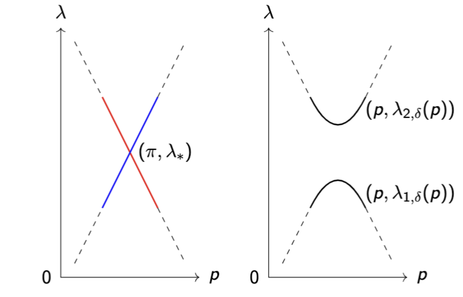
Figure 4: Lifting of the degeneracy near the Dirac point.

The following corollary states the existence of the common band gap for $\sigma(\mathcal{L}_{\delta})$ and $\sigma(\mathcal{L}_{-\delta})$:

Corollary 3.9 (The common band gap of $\sigma(\mathcal{L}_{\delta})$ and $\sigma(\mathcal{L}_{-\delta})$).

Let $\delta>0$ and $0<c<1$ be a constant. We follow all the notations and assumptions in Theorem 3.6 and define the real interval

$$I_{\delta}=(E_{1,\delta},E_{2,\delta}):=\left(\lambda_{*}-c\delta|\beta_{*}|,\lambda_{*}+c\delta|\beta_{*}|\right),$$ (3.20)

where $\beta_{*}=\frac{t_{*}}{\gamma_{*}}$. Then there exists $\delta_{0}>0$, such that for all $0<\delta<\delta_{0}$, there holds

$$I_{\delta}\bigcap\sigma(\mathcal{L}_{\delta})=I_{\delta}\bigcap\sigma(\mathcal{L}_{-\delta})=\emptyset.$$

Proof.

We only consider $\mathcal{L}_{\delta}$, and the proof for $\mathcal{L}_{-\delta}$ is identical. From Theorem 3.6, for any $c\in(0,1)$, there exists $\delta_{0}>0$ such that for all $0<\delta<\delta_{0}$, the dispersion relations $\lambda_{1,\delta}(p)$ and $\lambda_{2,\delta}(p)$ satisfy

$$\max_{|p-p_{*}|\leq\delta}\lambda_{1,\delta}(p)\leq\lambda_{*}-c\delta\beta_{*},\quad\min_{|p-p_{*}|\leq\delta}\lambda_{2,\delta}(p)\geq\lambda_{*}+c\delta\beta_{*}.$$

Thus to show that $I_{\delta}$ is indeed a band gap, it suffices to show that for $p\in\mathcal{B}\bigcap\left\{p:|p-\pi|\geq\delta\right\}$, $\lambda_{1,\delta}(p),\lambda_{2,\delta}(p)\notin I_{\delta}$, and $\lambda_{n,\delta}(p)\notin I_{\delta}$ for all $n\geq 3$ and $p\in\mathcal{B}$. Indeed, this follows from Assumption 1.1 that only the first and second dispersion curves touch at the Dirac point $(p_{*},\lambda_{*})$, and they are away from $\lambda=\lambda_{*}$ when $p\neq p_{*}$. ∎

3.3 Proof of Proposition 3.4 and Theorem 3.6

Proof of Theorem 3.6.

For ease of presentation, we assume that the constants $\theta_{*},\gamma_{*}$ and $t_{*}$ defined in Proposition 3.3 and 3.5 are all positive. Recall Remark 3.7 that such an assumption is not essential.

We first show that for each $p$ near $\pi$ and small $\delta$, the operator $T_{\delta}(\lambda;p):=T_{\delta}(p,\lambda)$ has two characteristic values (counted with multiplicity) with $|\lambda-\lambda_{*}|\ll 1$. To this end, it is sufficient to consider $p=\pi$, while the cases of $p\neq\pi$ can be treated similarly.

Note the characteristic values of $T(\lambda;p_{*})$ correspond to the Bloch eigenvalues of the problem (3.2) at $p=p_{*}$ and $\delta=0$. There is a small neighborhood $U(\lambda_{*})$ of $\lambda=\lambda_{*}$ in the complex plane such that $\lambda_{*}$ is the only characteristic value of $T(\lambda;p_{*})$ inside $\overline{U(\lambda_{*})}$ and its multiplicity is two. The analyticity of $T(\lambda;p_{*})$ in the variable $\lambda$ (See Lemma 3.2) implies that $T(\lambda;p_{*})$ is normal with respect to $\partial U(\lambda_{*})$, so does $T_{\delta}(\lambda;p_{*})$. On the other hand, by Lemma 3.2, $\|T(\lambda;p_{*})^{-1}(T(\lambda;p_{*})-T_{\delta}(\lambda;p_{*}))\|<1$ for $\lambda\in\partial U(\lambda_{*})$ for $\delta$ sufficiently small. Then Theorem 2.9 implies that $T_{\delta}(\lambda;p_{*})$ attains two characteristic values (counted with multiplicity) for $\lambda\in U(\lambda_{*})$.

Next, we calculate the asymptotic expansion of the characteristic values of $T_{\delta}(\lambda;p)$ and their associated eigenvectors by a perturbation argument.

Step 1. We first set up the framework to conduct the perturbation. In the vicinity of the Dirac point $(p_{*},\lambda_{*})$, we write the quasi-momentum as

$$p=p_{*}+p^{(1)},$$ (3.21)

where $|p^{(1)}|\ll 1$. We seek a solution to (3.7) of the form

$$\qquad\qquad\qquad\qquad\qquad\qquad\qquad\lambda(p_{*}+p^{(1)})=\lambda_{*}+\lambda^{(1)},$$ (3.22)

$$\bm{\varphi}(x;p_{*}+p^{(1)})=\bm{\varphi}^{(0)}+\bm{\varphi}^{(1)},\quad\bm{\varphi}^{(0)}=a\bm{\varphi_{1}}+b\bm{\varphi_{2}}\in\text{Ker}\,T(p_{*},\lambda_{*}),\quad\bm{\varphi}^{(1)}\in(\text{Ker}\,T(p_{*},\lambda_{*}))^{\perp},$$

where $|\lambda^{(1)}|\ll 1$, and $(\text{Ker}\,T(p_{*},\lambda_{*}))^{\perp}$ is the orthogonal complement of $\text{Ker}\,T(p_{*},\lambda_{*})$ in $H^{-\frac{1}{2}}(\partial D)\times H^{-\frac{1}{2}}(\partial D)$ . Here $\bm{\varphi_{1}}$ and $\bm{\varphi_{2}}$ are defined in Corollary 1.8.

Substituting (3.13), (3.21) and (3.22) into (3.7), we obtain the following equation for $\bm{\varphi}^{(1)}$:

$$T(p_{*},\lambda_{*})\bm{\varphi}^{(1)}= -\left(p^{(1)}T_{p}+\lambda^{(1)}T_{\lambda}+\delta S+\mathcal{O}((p^{(1)})^{2},(\lambda^{(1)})^{2},\delta^{2})\right)\bm{\varphi}^{(0)}$$ (3.23)

$$-\left(p^{(1)}T_{p}+\lambda^{(1)}T_{\lambda}+\delta S+\mathcal{O}((p^{(1)})^{2},(\lambda^{(1)})^{2},\delta^{2})\right)\bm{\varphi}^{(1)}.$$

Step 2. We solve (3.23) by following a Lyapunov-Schmidt reduction argument. Since $\text{Ran}\,(T(p_{*},\lambda_{*}))$ is closed in $H^{\frac{1}{2}}(\partial D)\times H^{\frac{1}{2}}(\partial D)$, we introduce the orthogonal projection $Q:H^{\frac{1}{2}}(\partial D)\times H^{\frac{1}{2}}(\partial D)\to\text{Ran}\,(T(p_{*},\lambda_{*}))$. By applying $Q$ to (3.23), we obtain

$$T(p_{*},\lambda_{*})\bm{\varphi}^{(1)}= -Q\left(p^{(1)}T_{p}+\lambda^{(1)}T_{\lambda}+\delta S+\mathcal{O}((p^{(1)})^{2},(\lambda^{(1)})^{2},\delta^{2})\right)\bm{\varphi}^{(0)}$$ (3.24)

$$-Q\left(p^{(1)}T_{p}+\lambda^{(1)}T_{\lambda}+\delta S+\mathcal{O}((p^{(1)})^{2},(\lambda^{(1)})^{2},\delta^{2})\right)\bm{\varphi}^{(1)}.$$

By Lemma 3.1, $T^{-1}(p_{*},\lambda_{*})\in\mathcal{B}(\text{Ran}\,(T(p_{*},\lambda_{*})),(\text{Ker}\,T(p_{*},\lambda_{*}))^{\perp})$. Then (3.24) can be rewritten as

$$(I+A)\bm{\varphi}^{(1)}=-A\bm{\varphi}^{(0)},$$ (3.25)

where the map $A$ is defined as

$$\bm{f}\mapsto A\bm{f}:=T^{-1}(p_{*},\lambda_{*})Q\left(p^{(1)}T_{p}+\lambda^{(1)}T_{\lambda}+\delta S+\mathcal{O}((p^{(1)})^{2},(\lambda^{(1)})^{2},\delta^{2})\right)\bm{f}.$$

Thus, for $p^{(1)},\lambda^{(1)},\delta$ sufficiently small, $(I+A)^{-1}$ exists, which implies that (3.25) is uniquely solvable:

$$\bm{\varphi}^{(1)}=-(I+A)^{-1}A\bm{\varphi}^{(0)}.$$ (3.26)

With (3.22), we may rewrite (3.26) as

$$\bm{\varphi}^{(1)}=\bm{\varphi}^{(1)}(x;p^{(1)},\lambda^{(1)},\delta)=\bm{g_{1}}(x;p^{(1)},\lambda^{(1)},\delta)a+\bm{g_{1}}(x;p^{(1)},\lambda^{(1)},\delta)b,$$

where the map $(p^{(1)},\lambda^{(1)},\delta)\mapsto\bm{g_{i}}(x;p^{(1)},\lambda^{(1)},\delta)$ ($i=1,2$) is smooth from a neighborhood of $(0,0,0)$ to $(\text{Ker}\,T(p_{*},\lambda_{*}))^{\perp}$ with the following estimate:

$$\left\|\bm{g_{i}}(x;p^{(1)},\lambda^{(1)},\delta)\right\|\lesssim|p^{(1)}|+|\lambda^{(1)}|+|\delta|.$$

Step 3. We take dual pair with $\bm{\varphi}_{i}$ ($i=1,2$) on both sides of (3.23). From the identity $\langle\overline{\bm{\psi}},T(p_{*},\lambda_{*})\bm{\varphi}\rangle=\overline{\langle\overline{\bm{\varphi}},T(p_{*},\lambda_{*})\bm{\psi}\rangle}$ for any $\bm{\varphi},\bm{\psi}$, we obtain the following equations for $(a,b)^{T}$:

$$\mathcal{M}(p^{(1)},\lambda^{(1)},\delta)\begin{pmatrix}a\\ b\end{pmatrix}=0,$$ (3.27)

with

$$\mathcal{M}(p^{(1)},\lambda^{(1)},\delta) :=\begin{pmatrix}\gamma_{*}\lambda^{(1)}+t_{*}\delta&-i\theta_{*}p^{(1)}\\ i\theta_{*}p^{(1)}&\gamma_{*}\lambda^{(1)}-t_{*}\delta\\ \end{pmatrix}\quad+\mathcal{O}((\lambda^{(1)})^{2},(p^{(1)})^{2},\delta^{2}).$$ (3.28)

Note that the higher-order term in (3.28) is smooth in $(p^{(1)},\lambda^{(1)},\delta)$ near $(0,0,0)$. Thus $(p,\lambda)$ with $\lambda=\lambda_{*}+\lambda^{(1)}(p^{(1)},\delta)$ is a characteristic value of $T_{\delta}(p,\lambda)$ defined in (3.7) if and only if $\lambda^{(1)}=\lambda^{(1)}(p^{(1)},\delta)$ solves the following equation

$$F(p^{(1)},\lambda^{(1)},\delta)\equiv\det\mathcal{M}(p^{(1)},\lambda^{(1)},\delta)=\gamma_{*}^{2}(\lambda^{(1)})^{2}-t_{*}^{2}\delta^{2}-\theta_{*}^{2}(p^{(1)})^{2}+\rho(p^{(1)},\lambda^{(1)},\delta)=0,$$ (3.29)

where $\rho(p^{(1)},\lambda^{(1)},\delta)$ is smooth near $(0,0,0)$ and satisfies

$$\left\|\rho(p^{(1)},\lambda^{(1)},\delta)\right\|=\mathcal{O}((\lambda^{(1)})^{3},(p^{(1)})^{3},\delta^{3}).$$ (3.30)

Step 4. We solve $\lambda^{(1)}=\lambda^{(1)}(p^{(1)},\delta)$ from (3.29) for each $p^{(1)}$ and $\delta$. We first note that $\pm\frac{1}{|\gamma_{*}|}\sqrt{t^{2}_{*}\delta^{2}+\theta^{2}_{*}(p^{(1)})^{2}}$ give two branches of solutions if we drop the remainder term $\rho$. Thus, we seek a solution to (3.29) in the following form

$$\lambda^{(1)}(p^{(1)},\delta)=\frac{x}{|\gamma_{*}|}\sqrt{t^{2}_{*}\delta^{2}+\theta^{2}_{*}(p^{(1)})^{2}}$$ (3.31)

with $|x|$ close to 1. It is clear that $x$ depends on $p^{(1)}$ and $\delta$. By substituting (3.31) into (3.29), we obtain the following equation of $x$, with $p^{(1)}$ and $\delta\neq 0$ being viewed as two parameters:

$$H(x;p^{(1)},\delta) :=\frac{1}{t^{2}_{*}\delta^{2}+\theta^{2}_{*}(p^{(1)})^{2}}F(p^{(1)},\frac{x}{|\gamma_{*}|}\sqrt{t^{2}_{*}\delta^{2}+\theta^{2}_{*}(p^{(1)})^{2}},\delta)$$ (3.32)

$$=x^{2}-1+\rho_{1}(x;p^{(1)},\delta)=0,$$

where $\rho_{1}(x;p^{(1)},\delta):=\frac{\rho(\frac{x}{|\gamma_{*}|}\sqrt{t^{2}_{*}\delta^{2}+\theta^{2}_{*}(p^{(1)})^{2}},p^{(1)},\delta)}{t^{2}_{*}\delta^{2}+\theta^{2}_{*}(p^{(1)})^{2}}$. Now we consider the upper branch of solution to (3.32) with $|x-1|\ll 1$. Note that the following estimates hold uniformly in $x$ by (3.30):

$$\left|\rho_{1}(x;p^{(1)},\delta)\right|=\mathcal{O}(p^{(1)},\delta).$$ (3.33)

We conclude that there exists a unique solution $x_{s}(p^{(1)},\delta)$ to the equation (3.32) with the estimate $x_{s}(p^{(1)},\delta)=1+\mathcal{O}(p^{1},\delta)$ for $\delta,|p^{(1)}|\ll 1$. It follows from (3.31) that there exists a unique solution $\lambda^{(1)}_{+}(p^{(1)},\delta)$ to the equation (3.29) near $\frac{1}{|\gamma_{*}|}\sqrt{t^{2}_{*}\delta^{2}+\theta^{2}_{*}(p^{(1)})^{2}}$. Moreover,

$$\lambda^{(1)}_{+}(p^{(1)},\delta)=\frac{x_{s}(p^{(1)},\delta)}{|\gamma_{*}|}\sqrt{t^{2}_{*}\delta^{2}+\theta^{2}_{*}(p^{(1)})^{2}})=\frac{1}{|\gamma_{*}|}\sqrt{t^{2}_{*}\delta^{2}+\theta^{2}_{*}(p^{(1)})^{2}})\left(1+\mathcal{O}(p^{(1)},\delta)\right).$$

Similarly, we can derive that

$$\lambda^{(1)}_{-}(p^{(1)},\delta)=-\frac{1}{|\gamma_{*}|}\sqrt{t^{2}_{*}\delta^{2}+\theta^{2}_{*}(p^{(1)})^{2}})\left(1+\mathcal{O}(p^{(1)},\delta)\right).$$

Note that $\lambda_{1,\delta}(p)=\lambda_{*}+\lambda^{(1)}_{+}(p-p_{*},\delta)$, $\lambda_{2,\delta}(p)=\lambda_{*}+\lambda^{(1)}_{-}(p-p_{*},\delta)$, whence (3.16) follows.

Step 5. Finally, by substituting $\lambda^{(1)}(p)=\lambda_{i,\delta}(p)-\lambda_{*}$ in (3.27) for $i=1,2$ respectively, one obtains the following solutions accordingly,

$$\begin{pmatrix}a_{1}\\ b_{1}\end{pmatrix}=\begin{pmatrix}1\\ \frac{\sqrt{-1}\theta_{*}(p-p_{*})}{\delta t_{*}+\sqrt{\delta^{2}t_{*}^{2}+\theta_{*}^{2}(p-p_{*})^{2}}}\end{pmatrix},\quad\begin{pmatrix}a_{2}\\ b_{2}\end{pmatrix}=\begin{pmatrix}\frac{\sqrt{-1}\theta_{*}(p-p_{*})}{\delta t_{*}+\sqrt{\delta^{2}t_{*}^{2}+\theta_{*}^{2}(p-p_{*})^{2}}}\\ 1\end{pmatrix}.$$

The asymptotic expansions of the eigenmodes $u_{i,\delta}(\cdot;p)$ in (3.17) are obtained by substituting $(a_{i},b_{i})^{T}$ above into (3.22) and then using the layer potentials in (3.5). The proof for (3.18) and (3.19) follows in a similar manner.

∎

Proof of Proposition 3.4.

The proposition is a consequence of Theorem 3.6. By letting $\delta=0$ in the asymptotic formula (3.16), we see that the first two dispersion functions of the unperturbed structure near $p=p^{*}$ admit the following expansions:

$$\lambda_{1}(p)=\lambda_{*}+\lambda^{(1)}_{-}(p-p_{*})=\lambda_{*}-\Big{|}\frac{\theta_{*}}{\gamma_{*}}\Big{|}|p-p_{*}|+\mathcal{O}((p-p_{*})^{2}),$$

$$\lambda_{2}(p)=\lambda_{*}+\lambda^{(1)}_{+}(p-p_{*})=\lambda_{*}+\Big{|}\frac{\theta_{*}}{\gamma_{*}}\Big{|}|p-p_{*}|+\mathcal{O}((p-p_{*})^{2}).$$

Therefore, the slope of the dispersion curve at the intersection point (which is the Dirac point) is $|\frac{\theta_{*}}{\gamma_{*}}|$. The slope is consistent with the one proposed in Proposition 1.5 and Assumption 1.1. Thus we have

$$\alpha_{*}=\Big{|}\frac{\theta_{*}}{\gamma_{*}}\Big{|}.$$

∎

4 Interface mode for the waveguide with perturbations

In this section, we prove the existence of an interface mode for the waveguide in Figure 2(c), as stated in Theorem 1.11. In Section 4.1, we reformulate the eigenvalue problem (1.6) as a boundary integral equation. The asymptotic expansions of the related boundary integral operators are derived with respect to the perturbation parameter $\delta$ in Section 4.2. Finally, we prove Theorem 1.11 in Section 4.3 by investigating the characteristic values of the associated boundary integral operator.

4.1 Boundary-integral formulation for the joint system with two semi-infinite perturbed media

In this subsection, we reformulate the eigenvalue problem (1.6) for the joint system in Figure 2(c) by using a boundary integral equation. The idea is to match the wave fields on both sides of the waveguide over the interface $\Gamma$. To proceed, we first introduce some notations. Recall that $\Gamma:=\{0\}\times(0,\frac{1}{2})$. Let $\tilde{\Gamma}:=\Gamma\cup\left([0,+\infty)\times\{0\}\right)\cup\left([0,+\infty)\times\{\frac{1}{2}\}\right)$ be the boundary of the semi-infinite waveguide $(0,+\infty)\times(0,\frac{1}{2})$. We define

$$H^{\frac{1}{2}}(\Gamma):=\{u=U|_{\Gamma}:U\in H^{\frac{1}{2}}(\tilde{\Gamma})\},$$

and

$$\tilde{H}^{-\frac{1}{2}}(\Gamma):=\{u=U|_{\Gamma}:U\in H^{-\frac{1}{2}}(\tilde{\Gamma})\text{ and }supp(U)\subset\overline{\Gamma}\}.$$

Then ${H}^{\frac{1}{2}}(\Gamma)$ is the dual space of $\tilde{H}^{-\frac{1}{2}}(\Gamma)$ and vice versa. We also denote the left and right domain in Figure 2(c) by $\tilde{\Omega}_{\delta}^{-}:=\tilde{\Omega}_{\delta}\bigcap\left((-\infty,0)\times(0,\frac{1}{2})\right)$ and $\tilde{\Omega}_{\delta}^{+}:=\tilde{\Omega}_{\delta}\bigcap\left((0,+\infty)\times(0,\frac{1}{2})\right)$, respectively.

Suppose that $u(x;\lambda)\in L^{2}(\tilde{\Omega}_{\delta})$ is a solution of the eigenvalue problem (1.6). We express $u(x;\lambda)$ as

$$u(x;\lambda)=\left\{\begin{aligned} &u^{+}(x),\quad x\in\tilde{\Omega}_{\delta}^{+},\\ &u^{-}(x),\quad x\in\tilde{\Omega}_{\delta}^{-},\end{aligned}\right.$$ (4.1)

where $u^{+}$ and $u^{-}$ satisfy respectively the following equations

$$\left\{\begin{aligned} &(\Delta_{x}+\lambda)u^{+}(x;\lambda)=0,\quad x\in\tilde{\Omega}_{\delta}^{+},\\ &u^{+}(x;\lambda)=0,\quad x\in\partial\tilde{D}_{n,\delta}\enspace(n=1,2,\cdots),\\ &\frac{\partial}{\partial x_{2}}u^{+}(x;\lambda)=0,\quad x\in\Gamma_{-}\bigcup\Gamma_{+}.\end{aligned}\right.\quad\left\{\begin{aligned} &(\Delta_{x}+\lambda)u^{-}(x;\lambda)=0,\quad x\in\tilde{\Omega}_{\delta}^{-},\\ &u^{-}(x;\lambda)=0,\quad x\in\partial\tilde{D}_{n,\delta}\enspace(n=-1,-2,\cdots),\\ &\frac{\partial}{\partial x_{2}}u^{-}(x;\lambda)=0,\quad x\in\Gamma_{-}\bigcup\Gamma_{+}.\end{aligned}\right.$$

For $\lambda\in I_{\delta}$, a common band gap for the left and the right periodic structures near the Dirac point $(p_{*},\lambda_{*})$, it is known that (see [22]) $u^{+}$ and $u^{-}$ decay exponentially away from the interface $\Gamma$ as $|x_{1}|\to\infty$ in $\tilde{\Omega}_{\delta}^{+}$ and $\tilde{\Omega}_{\delta}^{-}$ respectively. Moreover, the following interface conditions hold:

$$u(0^{-},x_{2};\lambda)=u(0^{+},x_{2};\lambda),$$ (4.2)

$$\frac{\partial u}{\partial x_{1}}(0^{-},x_{2};\lambda)=\frac{\partial u}{\partial x_{1}}(0^{+},x_{2};\lambda).$$ (4.3)

We have the following representation formulas for $u^{\pm}$.

Lemma 4.1.

Let $\lambda\in I_{\delta}$, then

$$u^{+}(x;\lambda)=2\int_{\Gamma}G_{\delta}(x,y;\lambda)\phi^{+}(y;\lambda)d\sigma(y),\quad\phi^{+}=\frac{\partial u^{+}}{\partial x_{1}}\Big{|}_{\Gamma},$$ (4.4)

$$u^{-}(x;\lambda)=-2\int_{\Gamma}G_{-\delta}(x,y;\lambda)\phi^{-}(y;\lambda)d\sigma(y),\quad\phi^{-}=\frac{\partial u^{-}}{\partial x_{1}}\Big{|}_{\Gamma},$$ (4.5)

where $G_{\pm\delta}(x,y;\lambda)$ is the Green’s function defined in (2.13). Moreover, for each $\phi\in\tilde{H}^{-\frac{1}{2}}(\Gamma)$, the following identity holds:

$$\left(\frac{\partial}{\partial x_{1}}\int_{\Gamma}G_{\delta}(x,y;\lambda)\phi(y)d\sigma(y)\right)(0^{+},x_{2})=\frac{\phi(x_{2})}{2}.$$ (4.6)

Proof.

We first prove the representation formula for $u^{+}$. The formula for $u^{-}$ can be proved similarly. Let $G_{\delta}^{\Gamma}$ be Green’s function in the perturbed semi-infinity waveguide with the Neumann boundary condition on $\Gamma$:

$$\left\{\begin{aligned} &(\Delta_{x}+\lambda)G^{\Gamma}_{\delta}(x,y;\lambda)=\tilde{\delta}(x-y),\quad x,y\in\Omega_{\delta},\\ &G^{\Gamma}_{\delta}(x,y;\lambda)=0,\quad x\in\cup_{n\geq 1}\partial D_{n,\delta},\\ &\frac{\partial}{\partial{x_{2}}}G^{\Gamma}_{\delta}(x,y;\lambda)=0,\quad x\in\Gamma_{-}\bigcup\Gamma_{+},\\ &\frac{\partial}{\partial{x_{1}}}G^{\Gamma}_{\delta}(x,y;\lambda)=0,\quad x\in\Gamma.\end{aligned}\right.$$

Since $\Omega_{\delta}$ attains reflection symmetry, for $y\in\Gamma$, there holds

$$G^{\Gamma}_{\delta}(x,y;\lambda)=\lim_{y_{1}\to 0^{-}}G_{\delta}(x,y;\lambda)+\lim_{y_{1}\to 0^{+}}G_{\delta}(x,y;\lambda)=2G_{\delta}(x,y;\lambda),$$

where $G_{\delta}(x,y;\lambda)$ is the Green’s function for the perturbed periodic structure defined in (2.13). Therefore, for $\lambda\in I_{\delta}$, $G^{\Gamma}_{\delta}(x,y;\lambda)$ decays exponentially for $|x_{1}|\to\infty$. Then an integration by parts yields

$$u^{+}(x;\lambda)=\int_{\Gamma}G^{\Gamma}_{\delta}(x,y;\lambda)\phi^{+}(y;\lambda)d\sigma(y)=2\int_{\Gamma}G_{\delta}(x,y;\lambda)\phi^{+}(y;\lambda)d\sigma(y),\quad\phi^{+}=\frac{\partial u^{+}}{\partial x_{1}}\Big{|}_{\Gamma},$$

whence the representation formula for $u^{+}$ follows.

Next, we show (4.6). Let $\left(\frac{\partial}{\partial x_{1}}\int_{\Gamma}G_{\delta}(x,y;\lambda)\phi(y)d\sigma(y)\right)(0^{+},x_{2})=\frac{\psi(x_{2})}{2}$. Then (4.4) gives

$$\int_{\Gamma}G_{\delta}(x,y;\lambda)\phi(y)d\sigma(y)=\int_{\Gamma}G_{\delta}(x,y;\lambda)\psi(y)d\sigma(y)\quad\mbox{for}\;x\in\Omega_{\delta}^{+}.$$ (4.7)

Define

$$u(x):=\int_{\Gamma}G_{\delta}(x,y;\lambda)(\phi(y)-\psi(y))d\sigma(y)\quad\mbox{for}\;x\in\Omega_{\delta}^{+}.$$ (4.8)

Then (4.7) implies that $u(x)\equiv 0$ for $x\in\Omega_{\delta}^{+}$. By the reflection symmetry of the Green’s function $G_{\delta}(x,y;\lambda)$ (which follows from the same arguments as in Lemma 2.4), $u(x)$ in (4.8) can be naturally extended to $x\in\Omega_{\delta}^{-}$. This gives an even extension of $u$, i.e. $u(x_{1},x_{2}):=u(-x_{1},x_{2})$ for $x_{1}<0$. Note that the extended $u(x)$ also vanishes in $\Omega_{\delta}$. On the other hand, if we rewrite $u$ as

$$u(x)=\int_{\Gamma}G_{\delta}(x,y;\lambda)(\phi(y)-\psi(y))d\sigma(y)=\int_{\Omega_{\delta}}G_{\delta}(x,y;\lambda)(\tilde{\phi}-\tilde{\psi})(y)dy,$$

where $(\tilde{\phi}-\tilde{\psi})(y):=\phi(y_{2})\tilde{\delta}(y_{1})-\psi(y_{2})\tilde{\delta}(y_{1})$ (here $\tilde{\delta}$ denotes the delta function), then

$$(\Delta+\lambda)u=\tilde{\phi}-\tilde{\psi}.$$

However, $(\Delta_{x}+\lambda)u\equiv 0$ for $u(x)\equiv 0$ when $x\in\Omega_{\delta}$. Hence we conclude that $\phi=\psi$ and Lemma 4.1 is proved. ∎

By Lemma 4.1 and (4.3), $u^{\pm}$ can be expressed as

$$u^{+}(x;\lambda)=2\int_{\Gamma}G_{\delta}(x,y;\lambda)\phi(y;\lambda)d\sigma(y),$$ (4.9)

$$u^{-}(x;\lambda)=-2\int_{\Gamma}G_{-\delta}(x,y;\lambda)\phi(y;\lambda)d\sigma(y),$$ (4.10)

for some $\phi\in\tilde{H}^{-\frac{1}{2}}(\Gamma)$. By substituting (4.9) and (4.10) into the interface condition (4.2), we obtain

$$2\int_{\Gamma}\left(G_{\delta}((0,x_{2}),(0,y_{2});\lambda)+G_{-\delta}((0,x_{2}),(0,y_{2});\lambda)\right)\phi((0,y_{2});\lambda)dy_{2}=0.$$ (4.11)

Let us introduce the following single-layer boundary integral operators

$$\mathbb{G}_{\pm\delta}(\lambda):\tilde{H}^{-\frac{1}{2}}(\Gamma)\to H^{\frac{1}{2}}(\Gamma),\quad\phi(y)\mapsto 2\int_{\Gamma}G_{\pm\delta}(x,y;\lambda)\phi(y;\lambda)dy,$$ (4.12)

and set

$$\tilde{\mathbb{G}}_{\delta}(\lambda):\tilde{H}^{-\frac{1}{2}}(\Gamma)\to H^{\frac{1}{2}}(\Gamma),\quad\tilde{\mathbb{G}}_{\delta}(\lambda)=\mathbb{G}_{\delta}(\lambda)+\mathbb{G}_{-\delta}(\lambda).$$

Then (4.11) is equivalent to the following boundary integral equation

$$\tilde{\mathbb{G}}_{\delta}(\lambda)\phi=0,\quad\mbox{for}\;\phi\in\tilde{H}^{-\frac{1}{2}}(\Gamma).$$ (4.13)

In summary, (1.6) attains an interface mode $u(x;\lambda)$, if and only if $\lambda\in I_{\delta}$ is a characteristic value of $\tilde{\mathbb{G}}_{\delta}(\lambda)$.

4.2 Properties of boundary integral operators

Here and henceforth, for each $\lambda\in I_{\delta}$, we parameterize $\lambda$ as $\lambda:=\lambda_{*}+\delta\cdot h$ for $h\in J:=(\frac{E_{1,\delta}-\lambda_{*}}{\delta},\frac{E_{2,\delta}-\lambda_{*}}{\delta})$. The complex neighborhood of $J$ is denoted by $\tilde{J}:=\{h\in\mathbb{C}:|h|<|\frac{E_{1,\delta}-E_{2,\delta}}{2\delta}|\}$.

We investigate the boundary integral operator $\tilde{\mathbb{G}}_{\delta}(\lambda_{*}+\delta\cdot h)=\mathbb{G}_{\delta}(\lambda_{*}+\delta\cdot h)+\mathbb{G}_{-\delta}(\lambda_{*}+\delta\cdot h)$ for $h\in\tilde{J}$. The results obtained will pave the way for applying the Gohberg and Sigal theory to prove Theorem 1.11.

To this end, we first define $\mathbb{T}_{\pm\delta}(\lambda_{*}+\delta\cdot h):\tilde{H}^{-\frac{1}{2}}(\Gamma)\to H^{\frac{1}{2}}(\Gamma)$ by

$$\mathbb{T}_{\pm\delta}(\lambda_{*}+\delta\cdot h)= \int_{0}^{2\pi}\sum_{n\geq 3}\frac{\langle\cdot,\overline{u_{n,\pm\delta}(y;p)}\rangle}{\lambda_{*}+\delta\cdot h-\lambda_{n,\pm\delta}(p)}u_{n,\pm\delta}(x;p)dp$$ (4.14)

$$+\int_{[0,\pi-\delta^{\frac{1}{3}}]\bigcup[\pi+\delta^{\frac{1}{3}},2\pi]}\frac{\langle\cdot,\overline{u_{2,\pm\delta}(y;p)}\rangle}{\lambda_{*}+\delta\cdot h-\lambda_{2,\pm\delta}(p)}u_{2,\pm\delta}(x;p)dp$$

$$+\int_{[0,\pi-\delta^{\frac{1}{3}}]\bigcup[\pi+\delta^{\frac{1}{3}},2\pi]}\frac{\langle\cdot,\overline{u_{1,\pm\delta}(y;p)}\rangle}{\lambda_{*}+\delta\cdot h-\lambda_{1,\pm\delta}(p)}u_{1,\pm\delta}(x;p)dp.$$

Here and henceforth, $\langle\cdot,\cdot\rangle$ denotes the duality pair on ${\tilde{H}^{-\frac{1}{2}}(\Gamma)\times H^{\frac{1}{2}}(\Gamma)}$.

Recall that $\phi_{1},\phi_{2}$ are the two Dirac eigenmodes, with $\phi_{1}$ being odd and $\phi_{2}$ being even (see Corollary 1.8). Let $\mathbb{P}$ be the projection operator defined by

$$\mathbb{P}:\tilde{H}^{-\frac{1}{2}}(\Gamma)\to H^{\frac{1}{2}}(\Gamma),\quad\psi\mapsto\langle\psi,\overline{\phi}_{2}\rangle\phi_{2}.$$

We further introduce the following four functions:

$$f_{1}(h;\delta):=\frac{1}{2\pi}\int_{\pi-\delta^{\frac{1}{3}}}^{\pi+\delta^{\frac{1}{3}}}\frac{1}{\delta\cdot h+\sqrt{\delta^{2}\beta_{*}^{2}+\alpha_{*}^{2}(p-p_{*})^{2}}}\frac{L(p;\delta)}{1+L(p;\delta)}dp,$$

$$f_{2}(h;\delta):=\frac{1}{2\pi}\int_{\pi-\delta^{\frac{1}{3}}}^{\pi+\delta^{\frac{1}{3}}}\frac{1}{\delta\cdot h-\sqrt{\delta^{2}\beta_{*}^{2}+\alpha_{*}^{2}(p-p_{*})^{2}}}\frac{1}{1+L(p;\delta)}dp,$$

$$\tilde{f}_{1}(h;\delta):=\frac{1}{2\pi}\int_{\pi-\delta^{\frac{1}{3}}}^{\pi+\delta^{\frac{1}{3}}}\frac{1}{\delta\cdot h+\sqrt{\delta^{2}\beta_{*}^{2}+\alpha_{*}^{2}(p-p_{*})^{2}}}\frac{1}{1+L(p;\delta)}dp,$$

$$\tilde{f}_{2}(h;\delta):=\frac{1}{2\pi}\int_{\pi-\delta^{\frac{1}{3}}}^{\pi+\delta^{\frac{1}{3}}}\frac{1}{\delta\cdot h-\sqrt{\delta^{2}\beta_{*}^{2}+\alpha_{*}^{2}(p-p_{*})^{2}}}\frac{L(p;\delta)}{1+L(p;\delta)}dp,$$

where

$$\alpha_{*}=\frac{\theta_{*}}{\gamma_{*}},\quad\beta_{*}=\frac{t_{*}}{\gamma_{*}},\quad L(p;\delta):=\frac{\alpha_{*}^{2}(p-p_{*})^{2}}{(\delta\beta_{*}+\sqrt{\delta^{2}\beta_{*}^{2}+\alpha_{*}^{2}(p-p_{*})^{2}})^{2}}.$$

We have the following asymptotic expansions of the operators $\mathbb{G}_{\pm\delta}$.

Proposition 4.2.

There exists $\delta_{0}>0$ such that for $0<\delta<\delta_{0}$, the operator $\mathbb{G}_{\delta}$ defined in (4.12) admits the following asymptotic expansion

$$\mathbb{G}_{\delta}(\lambda_{*}+\delta\cdot h)=\mathbb{T}_{\delta}(\lambda_{*}+\delta\cdot h)+\Big{(}f_{1}(h;\delta)+f_{2}(h;\delta)\Big{)}\mathbb{P}+\Big{(}\mathbb{R}_{1}(h;\delta)+\mathbb{R}_{2}(h;\delta)\Big{)},$$ (4.15)

where all functions and operators in (4.15) are analytic with respect to $h$ in $\tilde{J}$. Moreover, the following hold uniformly for $h\in\tilde{J}$:

$$\lim_{\delta\to 0}\|\mathbb{R}_{1}(h;\delta)\|_{\mathcal{B}(\tilde{H}^{-\frac{1}{2}}(\Gamma),H^{\frac{1}{2}}(\Gamma))}=0,\quad\lim_{\delta\to 0}\|\mathbb{R}_{2}(h;\delta)\|_{\mathcal{B}(\tilde{H}^{-\frac{1}{2}}(\Gamma),H^{\frac{1}{2}}(\Gamma))}=0.$$ (4.16)

Similarly,

$$\mathbb{G}_{-\delta}(\lambda_{*}+\delta\cdot h)=\mathbb{T}_{-\delta}(\lambda_{*}+\delta\cdot h)+\Big{(}\tilde{f}_{1}(h;\delta)+\tilde{f}_{2}(h;\delta)\Big{)}\mathbb{P}+\Big{(}\tilde{\mathbb{R}}_{1}(h;\delta)+\tilde{\mathbb{R}}_{2}(h;\delta)\Big{)},$$ (4.17)

with

$$\lim_{\delta\to 0}\|\tilde{\mathbb{R}}_{1}(h;\delta)\|_{\mathcal{B}(\tilde{H}^{-\frac{1}{2}}(\Gamma),H^{\frac{1}{2}}(\Gamma))}=0,\quad\lim_{\delta\to 0}\|\tilde{\mathbb{R}}_{2}(h;\delta)\|_{\mathcal{B}(\tilde{H}^{-\frac{1}{2}}(\Gamma),H^{\frac{1}{2}}(\Gamma))}=0.$$ (4.18)

Proof.

See Appendix D. ∎

We next investigate the limiting behavior of the operator $\mathbb{T}_{\pm\delta}$ as $\delta\to 0$. To this end, we define the following integral operator $\mathbb{T}_{0}\in\mathcal{B}(\tilde{H}^{-\frac{1}{2}}(\Gamma),H^{\frac{1}{2}}(\Gamma))$:

$$\mathbb{T}_{0}=\frac{1}{2\pi}\int_{0}^{2\pi}\sum_{n\geq 3}\frac{\langle\cdot,\overline{u_{n}(y;p)}\rangle}{\lambda_{*}-\lambda_{n}(p)}u_{n}(x;p)dp+\frac{1}{2\pi}p.v.\int_{0}^{2\pi}\sum_{n=1,2}\frac{\langle\cdot,\overline{v_{n}(y;p)}\rangle}{\lambda_{*}-\mu_{n}(p)}v_{n}(x;p)dp.$$

Using (2.2), the kernel function of the operator $\mathbb{T}_{0}$ (denoted by $T_{0}(x,y;\lambda_{*})$) is related to the Green’s function $G(x,y;\lambda_{*})$ by

$$G(x,y;\lambda_{*})=T_{0}(x,y;\lambda_{*})-\frac{i}{2}\frac{v_{1}(x,\pi)\overline{v_{1}(y,\pi)}}{\alpha_{*}}-\frac{i}{2}\frac{v_{2}(x,\pi)\overline{v_{2}(y,\pi)}}{\alpha_{*}}.$$ (4.19)

The following two propositions give the properties of the operator $\mathbb{T}_{0}$.

Proposition 4.3.

The kernel of $\mathbb{T}_{0}$ is given by

$$\text{Ker}\,\mathbb{T}_{0}=\text{span}\left\{\frac{\partial v_{1}}{\partial x_{1}}\big{|}_{\Gamma}\right\}.$$ (4.20)

Proposition 4.4.

$\mathbb{T}_{0}\in\mathcal{B}(\tilde{H}^{-\frac{1}{2}}(\Gamma),H^{\frac{1}{2}}(\Gamma))$ is a Fredholm operator of index zero.

Proof.

See Appendix E. ∎

We are now ready to investigate the limit of the operator $\tilde{\mathbb{G}}_{\delta}(\lambda_{*}+\delta\cdot h)$.

Proposition 4.5.

The following holds uniformly for $h\in\tilde{J}$:

$$\lim_{\delta\to 0}\Bigg{\|}\tilde{\mathbb{G}}_{\delta}(\lambda_{*}+\delta\cdot h)-\Big{(}2\mathbb{T}_{0}+\beta(h)\mathbb{P}\Big{)}\Bigg{\|}_{\mathcal{B}(\tilde{H}^{-\frac{1}{2}}(\Gamma),H^{\frac{1}{2}}(\Gamma))}=0,$$

where

$$\beta(h)=-\frac{1}{\beta_{*}\alpha_{*}}\frac{h}{\sqrt{1-(\frac{h}{\beta_{*}})^{2}}}.$$

Proof.

See Appendix F. ∎

Denote the limiting operator above by $\tilde{\mathbb{G}}_{0}(h):=2\mathbb{T}_{0}+\beta(h)\mathbb{P}$. We have

Proposition 4.6.

Let $h\in\tilde{J}$. Then $\tilde{\mathbb{G}}_{0}(h)$ is a Fredholm operator with index zero, analytic for $h\in\tilde{J}$, and continuous for $h\in\partial\tilde{J}$. As a function of $h$, it attains a unique characteristic value $h=0$ in $\tilde{J}$, whose null multiplicity is one. Moreover, $\tilde{\mathbb{G}}_{0}(h)$ is invertible for any $h\in\tilde{J}$ with $h\neq 0$.

Proof.

First, by the boundedness of $\mathbb{T}_{0}$ and $\mathbb{P}$, $\tilde{\mathbb{G}}_{0}(h)\in\mathcal{B}(\tilde{H}^{-\frac{1}{2}}(\Gamma),H^{\frac{1}{2}}(\Gamma))$. By selecting the principal branch of the square root on $\mathbb{C}\backslash(-\infty,-\beta_{*})\bigcup(\beta_{*},+\infty)$, it is clear that $\beta(h)$ is analytic on $\tilde{J}$, which implies the analyticity of $\tilde{\mathbb{G}}_{0}(h)$ as seen by its definition; then its continuity for $h\in\partial\tilde{J}$ is also clear. By Proposition 4.3, we deduce that $\mathbb{T}_{0}\in\mathcal{B}(\tilde{H}^{-\frac{1}{2}}(\Gamma),H^{\frac{1}{2}}(\Gamma))$ is a Fredholm operator with zero index and $\text{Ker}\,\mathbb{T}_{0}=\text{span}\left\{\frac{\partial v_{1}}{\partial x_{1}}\big{|}_{\Gamma}\right\}$. Thus $\tilde{\mathbb{G}}_{0}(h)$, which is obtained by perturbing $\mathbb{T}_{0}$ with the rank-1 projection operator $\mathbb{P}$, is a Fredholm operator with zero index.

Now we show that, as a function of $h$, $\tilde{\mathbb{G}}_{0}(h)=2\mathbb{T}_{0}+\beta(h)\mathbb{P}$ attains a unique characteristic value $h=0$ in $\tilde{J}$. In another word, the following equation attains a nontrivial solution $w\in\tilde{H}^{-\frac{1}{2}}(\Gamma)$ if and only if $h=0$:

$$\tilde{\mathbb{G}}_{0}(h)w=0.$$ (4.21)

To this end, we apply $\frac{\partial\overline{v_{1}}}{\partial x_{1}}\Big{|}_{\Gamma}$ to both hand sides of the equation above to get

$$0 =2\left\langle\frac{\partial\overline{v_{1}}}{\partial x_{1}}\Big{|}_{\Gamma},\mathbb{T}_{0}w\right\rangle+\langle w,\overline{\phi_{2}}\rangle\beta(h)\left\langle\frac{\partial\overline{v_{1}}}{\partial x_{1}}\Big{|}_{\Gamma},\phi_{2}\right\rangle$$

$$=2\overline{\left\langle\overline{w},\mathbb{T}_{0}\Big{(}\frac{\partial v_{1}}{\partial x_{1}}\Big{)}\Big{|}_{\Gamma}\right\rangle}+\langle w,\overline{\phi_{2}}\rangle\beta(h)\left\langle\frac{\partial\overline{v_{1}}}{\partial x_{1}}\Big{|}_{\Gamma},\phi_{2}\right\rangle$$

$$=\langle w,\overline{\phi_{2}}\rangle\beta(h)\left\langle\frac{\partial\overline{v_{1}}}{\partial x_{1}}\Big{|}_{\Gamma},\phi_{2}\right\rangle.$$

where the second identity follows from the definition of $\mathbb{T}_{0}$. Recall the fact that $\phi_{2}|_{\Gamma}$ is proportional to $v_{1}|_{\Gamma}$ (See Remark 1.9). As a result,

$$\langle w,\overline{\phi_{2}}\rangle\beta(h)\left\langle\frac{\partial\overline{v_{1}}}{\partial x_{1}}\Big{|}_{\Gamma},v_{1}\right\rangle=0.$$ (4.22)

By Lemma 2.3, $\Big{\langle}\frac{\partial\overline{v_{1}}}{\partial x_{1}}\Big{|}_{\Gamma},v_{1}\Big{\rangle}\neq 0$; thus (4.22) implies $\langle w,\overline{\phi_{2}}\rangle\beta(h)=0$, or equivalently

$$\langle w,\overline{v_{1}}\rangle\beta(h)=0.$$

If $\beta(h)\neq 0$, we have $\langle w,\overline{v_{1}}\rangle=0$ and $\mathbb{T}_{0}w=0$, which imply that $w=0$ by Proposition 4.3. But this contradicts the assumption that $w\neq 0$. Hence, we deduce that the characteristic value problem (4.21) attains solutions only when $\beta(h)=0$. Solving $\beta(h)=0$, we obtain a simple root $h=0$. Then Proposition 4.3 implies that $h=0$ is a characteristic value of multiplicity one with its associated eigenvector $\frac{\partial v_{1}}{\partial x_{1}}\Big{|}_{\Gamma}$.

Finally, we prove the invertibility of $\tilde{\mathbb{G}}_{0}(h)$ for $h\neq 0$. Indeed, since $\tilde{\mathbb{G}}_{0}(h)$ has a unique characteristic value $h=0$, it is injective for $h\neq 0$; thus, $\tilde{\mathbb{G}}_{0}(h)$ is invertible by noting that it is a Fredholm operator of zero index. ∎

Proposition 4.7.

Let $h\in\tilde{J}$. Then $\tilde{\mathbb{G}}_{\delta}(\lambda_{*}+\delta\cdot h)$ is a Fredholm operator, and it is analytic for $h\in\tilde{J}$.

Proof.

The analyticity of $\tilde{\mathbb{G}}_{\delta}(\lambda_{*}+\delta\cdot h)$ follows from the analyticity of the Green’s function $G_{\delta}(x,y;\lambda)$ in $\lambda$, which holds for any $\lambda=\lambda_{*}+\delta\cdot h$ with $h\in\tilde{J}$. Using Proposition 4.5 and 4.6, and the fact that Fredholm index is stable under small perturbation (see Proposition 2.8), we conclude that $\tilde{G}_{\delta}(\lambda_{*}+\delta\cdot h)$ is a Fredholm operator with zero index for $h\in\tilde{J}$ when $\delta>0$ is sufficiently small. ∎

4.3 Proof of Theorem 1.11

By Propositions 4.5 and 4.6, for sufficiently small $\delta>0$ and $h\in\partial\tilde{J}$, we have

$$\Bigg{\|}\tilde{\mathbb{G}}^{-1}_{0}(h)\Big{(}\tilde{\mathbb{G}}_{\delta}(\lambda_{*}+\delta\cdot h)-\tilde{\mathbb{G}}_{0}(h)\Big{)}\Bigg{\|}_{\mathcal{B}(\tilde{H}^{-\frac{1}{2}}(\Gamma))}<1,$$

where we have used the fact that $\tilde{\mathbb{G}}^{-1}_{0}(h)$ is uniformly bounded in norm for $h\in\partial\tilde{J}$ (it is a direct consequence of the continuity and invertibility of $\tilde{\mathbb{G}}_{0}(h)$ for $h\in\partial\tilde{J}$). Now, with Proposition 4.6 and 4.7, an application of Theorem 2.9 shows that, for sufficiently small $\delta>0$, (4.13) attains a unique characteristic value $\lambda^{\star}:=\lambda_{*}+h^{\star}$ with $h^{\star}\in\tilde{J}$. Let $\phi^{\star}$ be the associated eigenvector, then we construct a solution to (1.6) by setting

$$\lambda=\lambda^{\star},\quad u^{\star}=u((x_{1},x_{2});\lambda^{\star})=\left\{\begin{aligned} &\int_{\Gamma}G_{\delta}((x_{1},x_{2}),y;\lambda)\phi^{\star}(y;\lambda)d\sigma(y),\quad x_{1}\geq 0,\\ &-\int_{\Gamma}G_{-\delta}((x_{1},x_{2}),y;\lambda)\phi^{\star}(y;\lambda)d\sigma(y),\quad x_{1}<0.\end{aligned}\right.$$

Meanwhile, we claim that $\lambda^{\star}\in\mathbf{R}$. Otherwise, $(\overline{\lambda^{\star}},\overline{u^{\star}})$ gives another solution to the eigenvalue problem (1.6) and thus, $\overline{h}=\frac{\overline{\lambda^{\star}}-\lambda_{*}}{\delta}$ is another characteristic value of $\tilde{\mathbb{G}}_{\delta}(\lambda_{*}+\delta\cdot h)$ for $h\in\tilde{J}$, which is different from $h^{\star}$. But this contradicts the uniqueness of the characteristic value of $\tilde{\mathbb{G}}_{\delta}(\lambda_{*}+\delta\cdot h)$ for $h\in\tilde{J}$.

Finally, the assertion that $u^{\star}$ decays exponentially away from $\Gamma$ follows from the radiation condition of the Green’s function $G_{\pm\delta}$ (See Section 2.3). This completes the proof of the theorem.

Appendix A Appendix

Appendix A: Proof of Corollary 1.8

Proof of Corollary 1.8.

Let $v_{1}(x)=\text{Re }v_{1}(x)+i\,\text{Im }v_{1}(x)$. We first claim that $\text{Re }v_{1}(x)$ and $\text{Im }v_{1}(x)$ are linearly independent. Otherwise, there exists $c\in\mathbf{R}$ such that $\text{Re }v_{1}(x)=c\,\text{Im }v_{1}(x)$. Then the quasi-periodic boundary condition $v_{1}(x+\frac{1}{2}\bm{e_{1}})=iv_{1}$ gives

$$v_{1}(x+\frac{1}{2}\bm{e_{1}})=\text{Re }v_{1}(x+\frac{1}{2}\bm{e_{1}})+i\text{Im }v_{1}(x+\frac{1}{2}\bm{e_{1}})=(c+i)\text{Im }v_{1}(x+\frac{1}{2}\bm{e_{1}}),$$

$$v_{1}(x+\frac{1}{2}\bm{e_{1}})=iv_{1}(x)=i(\text{Re }v_{1}(x)+i\text{Im }v_{1}(x))=i(c+i)\text{Im }v_{1}(x),$$

which implies that $i\,\text{Im }v_{1}(x)=\text{Im }v_{1}(x+\frac{1}{2}\bm{e_{1}})$, and thus $\text{Im }v_{1}(x)=\text{Re }v_{1}(x)=0$. This contradiction proves the claim.

We next show that the desired even/odd eigenmodes at the Dirac point can be constructed by using linear combinations of $\text{Re }v_{1}$ and $\text{Im }v_{1}$. It is clear that both $\text{Re }v_{1}$ and $\text{Im }v_{1}$ are eigenmodes at the Dirac point defined in Proposition 1.5. Note that both $\overline{v_{1}(x_{1},x_{2})}$ and $v_{1}(-x_{1},x_{2})$ are Bloch eigenmodes with the same quasi-periodic boundary condition in the period-$\frac{1}{2}$ structure. Since the dimension of the eigenspace is one by Assumption 1.1, there exists $\theta\in[0,2\pi)$ such that $\overline{v_{1}(x_{1},x_{2})}=e^{i\theta}v_{1}(-x_{1},x_{2})$. Set $R:=\begin{pmatrix}\cos\theta&-\sin\theta\\ -\sin\theta&-\cos\theta\end{pmatrix}$. Then we have

$$\begin{pmatrix}\text{Re }v_{1}(x_{1},x_{2})\\ \text{Im }v_{1}(x_{1},x_{2})\end{pmatrix}=R\begin{pmatrix}\text{Re }v_{1}(-x_{1},x_{2})\\ \text{Im }v_{1}(-x_{1},x_{2})\end{pmatrix}.$$

The real matrix $R$ has two eigenvalues, $-1$ and $1$. Let $(a_{1},b_{1})^{T},(a_{2},b_{2})^{T}\in\mathbf{R}^{2}$ be the corresponding real eigenvectors, i.e.,

$$R(a_{1},b_{1})^{T}=-(a_{1},b_{1})^{T},\quad R(a_{2},b_{2})^{T}=(a_{2},b_{2})^{T}.$$

We define

$$\phi_{1}:=a_{1}\text{Re }v_{1}+b_{1}\text{Im }v_{1},\quad\phi_{2}:=a_{2}\text{Re }v_{1}+b_{2}\text{Im }v_{1}.$$

Then one can check that $\phi_{1}(-x_{1},x_{2})=-\phi_{1}(x_{1},x_{2})$, $\phi_{2}(-x_{1},x_{2})=\phi_{2}(x_{1},x_{2})$. This gives the desired construction.

Finally, note that $\phi_{1}$ is real-valued. Thus, the quasi-periodicity of $\phi_{1}$ and reflection-symmetry allows us to set the corresponding boundary potential $\bm{\varphi_{1}}$ as

$$\bm{\varphi_{1}}=(\varphi_{ref},\varphi)^{T},$$

where $\varphi\in H^{-\frac{1}{2}}(\partial D)$ is real-valued. Taking the reflection image of $\phi_{1}$ with respect to the straight line $x_{1}=\frac{1}{4}$, we obtain an even mode $\phi_{2}$ with the boundary potential

$$\bm{\varphi_{2}}=(\varphi,-\varphi_{ref})^{T}.$$

Then the proof is completed. ∎

Appendix B: Proof of Proposition 3.3

In Appendix B-C, the bracket $\langle\cdot,\cdot\rangle$ denotes the dual pair between $H^{-\frac{1}{2}}(\partial D)\times H^{-\frac{1}{2}}(\partial D)$ and $H^{\frac{1}{2}}(\partial D)\times H^{\frac{1}{2}}(\partial D)$.

Proof.

Step 1. First we show that for $(p,\lambda)$ near $(\pi,\lambda_{*})$,

$$\langle\bm{\varphi},T(p,\lambda)\bm{\varphi}\rangle=\overline{\langle\bm{\varphi},T(p,\lambda)\bm{\varphi}\rangle}\text{ for real-valued $\bm{\varphi}$}.$$ (B.1)

Note that the quasi-periodic Green’s function for the empty waveguide defined in (3.3) has the following properties:

$$G^{e}(x,y;\pi+h_{p},\lambda_{*})=\overline{G^{e}(x,y;\pi-h_{p},\lambda_{*})},$$ (B.2)

$$G^{e}(x,y;\pi+h_{p},\lambda_{*}+h_{\lambda})=\overline{G^{e}(y,x;\pi+h_{p},\lambda_{*}+h_{\lambda})},$$

for sufficiently small constants $h_{p},h_{\lambda}$. Using the polar coordinate for the boundary $\partial D$ and Corollary 1.8, we have

$$\langle\bm{\varphi},T(p,\lambda)\bm{\varphi}\rangle=V_{1}(p,\lambda)+V_{2}(p,\lambda)+V_{3}(p,\lambda)+V_{4}(p,\lambda),$$

where

$$V_{1}(p,\lambda) =\int_{[0,2\pi]\times[0,2\pi]}G^{e}(\bm{r}(\theta_{1}),\bm{r}(\theta_{2});p,\lambda)\cdot\varphi_{1}(\theta_{2})\varphi_{1}(\theta_{1})\cdot|\bm{r}^{\prime}(\theta_{2})||\bm{r}^{\prime}(\theta_{1})|d\theta_{2}d\theta_{1},$$

$$V_{2}(p,\lambda) =\int_{[0,2\pi]\times[0,2\pi]}G^{e}(\bm{r}(\theta_{1}),\frac{1}{2}\bm{e}_{1}+\bm{r}(\theta_{2});p,\lambda)\cdot\varphi_{2}(\theta_{2})\varphi_{1}(\theta_{1})\cdot|\bm{r}^{\prime}(\theta_{2})||\bm{r}^{\prime}(\theta_{1})|d\theta_{2}d\theta_{1},$$

$$V_{3}(p,\lambda) =\int_{[0,2\pi]\times[0,2\pi]}G^{e}(\frac{1}{2}\bm{e}_{1}+\bm{r}(\theta_{1}),\bm{r}(\theta_{2});p,\lambda)\cdot\varphi_{1}(\theta_{2})\varphi_{2}(\theta_{1})\cdot|\bm{r}^{\prime}(\theta_{2})||\bm{r}^{\prime}(\theta_{1})|d\theta_{2}d\theta_{1},$$

$$V_{4}(p,\lambda) =\int_{[0,2\pi]\times[0,2\pi]}G^{e}(\bm{r}(\theta_{1}),\bm{r}(\theta_{2});p,\lambda)\cdot\varphi_{2}(\theta_{2})\varphi_{2}(\theta_{1})\cdot|\bm{r}^{\prime}(\theta_{2})||\bm{r}^{\prime}(\theta_{1})|d\theta_{2}d\theta_{1}.$$

We claim that $V_{1},V_{4}$, and $V_{2}+V_{3}$ are all real numbers. For $V_{1}$, a change of variable yields

$$2V_{1}(p,\lambda)= \int_{[0,2\pi]\times[0,2\pi]}G^{e}(\bm{r}(\theta_{1}),\bm{r}(\theta_{2});p,\lambda)\cdot\varphi_{1}(\theta_{2})\varphi_{1}(\theta_{1})\cdot|\bm{r}^{\prime}(\theta_{2})||\bm{r}^{\prime}(\theta_{1})|d\theta_{2}d\theta_{1}$$

$$+\int_{[0,2\pi]\times[0,2\pi]}G^{e}(\bm{r}(\theta_{2}),\bm{r}(\theta_{1});p,\lambda)\cdot\varphi_{1}(\theta_{1})\varphi_{1}(\theta_{2})\cdot|\bm{r}^{\prime}(\theta_{1})||\bm{r}^{\prime}(\theta_{2})|d\theta_{1}d\theta_{2}$$

$$= \int_{[0,2\pi]\times[0,2\pi]}\Big{(}G^{e}(\bm{r}(\theta_{1}),\bm{r}(\theta_{2}))+G^{e}(\bm{r}(\theta_{2}),\bm{r}(\theta_{1}))\Big{)}\varphi_{1}(\theta_{2})\varphi_{1}(\theta_{1})|\bm{r}^{\prime}(\theta_{2})||\bm{r}^{\prime}(\theta_{1})|d\theta_{2}d\theta_{1}.$$

Thus (B.2) shows that the integrand of $V_{1}(p,\lambda)$ is real, which implies that $V_{1}(p,\lambda)\in\mathbf{R}$. Similarly, it can be proved that $V_{4}(p,\lambda)\in\mathbf{R}$. Besides,

$$V_{2}(p,\lambda)+V_{3}(p,\lambda)=\int_{[0,2\pi]\times[0,2\pi]}G^{e}(\bm{r}(\theta_{1}),\frac{1}{2}\bm{e}_{1}+\bm{r}(\theta_{2});p,\lambda)\cdot\varphi_{2}(\theta_{2})\varphi_{1}(\theta_{1})\cdot|\bm{r}^{\prime}(\theta_{2})||\bm{r}^{\prime}(\theta_{1})|d\theta_{2}d\theta_{1}$$

$$\qquad\qquad\qquad\qquad\quad+\int_{[0,2\pi]\times[0,2\pi]}G^{e}(\frac{1}{2}\bm{e}_{1}+\bm{r}(\theta_{2}),\bm{r}(\theta_{1});p,\lambda)\cdot\varphi_{1}(\theta_{1})\varphi_{2}(\theta_{2})\cdot|\bm{r}^{\prime}(\theta_{1})||\bm{r}^{\prime}(\theta_{2})|d\theta_{1}d\theta_{2}$$

$$=\int_{[0,2\pi]\times[0,2\pi]}\Big{(}G^{e}(\bm{r}(\theta_{1}),\frac{1}{2}\bm{e}_{1}+\bm{r}(\theta_{2}))+G^{e}(\frac{1}{2}\bm{e}_{1}+\bm{r}(\theta_{2}),\bm{r}(\theta_{1}))\Big{)}\varphi_{1}(\theta_{1})\varphi_{2}(\theta_{2})|\bm{r}^{\prime}(\theta_{1})||\bm{r}^{\prime}(\theta_{2})|d\theta_{1}d\theta_{2},$$

which is also real by invoking (B.2). Thus, $\langle\bm{\varphi},T(p,\lambda)\bm{\varphi}\rangle$ is real for any real-valued $\bm{\varphi}$.

Step 2. We prove that $\langle\bm{\varphi_{1}},T_{p}\bm{\varphi_{1}}\rangle=0$, and in a similar way $\langle\bm{\varphi_{2}},T_{p}\bm{\varphi_{2}}\rangle=0$. From (B.2), we have

$$\langle\bm{\varphi_{1}},T(p_{*}+h,\lambda_{*})\bm{\varphi_{1}}\rangle=\langle\bm{\varphi_{1}},\overline{T(p_{*}-h,\lambda_{*})}\bm{\varphi_{1}}\rangle.$$

Moreover, since $\bm{\varphi}_{1}$ is real-valued, (B.1) gives that

$$\langle\bm{\varphi_{1}},\overline{T(p_{*}-h,\lambda_{*})}\bm{\varphi_{1}}\rangle=\overline{\langle\bm{\varphi_{1}},T(p_{*}-h,\lambda_{*})\bm{\varphi_{1}}\rangle}=\langle\bm{\varphi_{1}},T(p_{*}-h,\lambda_{*})\bm{\varphi_{1}}\rangle.$$

In conclusion,

$$\langle\bm{\varphi_{1}},T(p_{*}+h,\lambda_{*})\bm{\varphi_{1}}\rangle=\langle\bm{\varphi_{1}},T(p_{*}-h,\lambda_{*})\bm{\varphi_{1}}\rangle.$$

Then by the smoothness of $\langle\bm{\varphi_{1}},T(p,\lambda_{*})\bm{\varphi_{1}}\rangle$ in $p$ near $p=\pi$, we obtain $\langle\bm{\varphi_{1}},T_{p}\bm{\varphi_{1}}\rangle=0$.

Step 3. We show that $\langle\bm{\varphi_{1}},T_{p}\bm{\varphi_{2}}\rangle=-\langle\bm{\varphi_{2}},T_{p}\bm{\varphi_{1}}\rangle$ is a pure imaginary number. First,

$$\langle\bm{\varphi_{2}},T(p,\lambda)\bm{\varphi_{1}}\rangle =\int_{[0,2\pi]\times[0,2\pi]}G^{e}(\bm{r}(\theta_{1}),\bm{r}(\theta_{2});p,\lambda)\cdot\varphi_{ref}(\theta_{2})\varphi(\theta_{1})\cdot|\bm{r}^{\prime}(\theta_{2})||\bm{r}^{\prime}(\theta_{1})|d\theta_{2}d\theta_{1}$$ (B.3)

$$\quad+\int_{[0,2\pi]\times[0,2\pi]}G^{e}(\bm{r}(\theta_{1}),\frac{1}{2}\bm{e}_{1}+\bm{r}(\theta_{2});p,\lambda)\cdot\varphi(\theta_{2})\varphi(\theta_{1})\cdot|\bm{r}^{\prime}(\theta_{2})||\bm{r}^{\prime}(\theta_{1})|d\theta_{2}d\theta_{1}$$

$$\quad-\int_{[0,2\pi]\times[0,2\pi]}G^{e}(\frac{1}{2}\bm{e}_{1}+\bm{r}(\theta_{1}),\bm{r}(\theta_{2});p,\lambda)\cdot\varphi_{ref}(\theta_{2})\varphi_{ref}(\theta_{1})\cdot|\bm{r}^{\prime}(\theta_{2})||\bm{r}^{\prime}(\theta_{1})|d\theta_{2}d\theta_{1}$$

$$\quad-\int_{[0,2\pi]\times[0,2\pi]}G^{e}(\bm{r}(\theta_{1}),\bm{r}(\theta_{2});p,\lambda)\cdot\varphi(\theta_{2})\varphi_{ref}(\theta_{1})\cdot|\bm{r}^{\prime}(\theta_{2})||\bm{r}^{\prime}(\theta_{1})|d\theta_{2}d\theta_{1}$$

$$=:U_{1}(p,\lambda)+U_{2}(p,\lambda)+U_{3}(p,\lambda)+U_{4}(p,\lambda).$$

Note that the Green’s function $G^{e}$ can be written in the following form

$$G^{e}(x,y;p,\lambda)=\sum_{n\in\mathbb{Z}}f(\lambda,|p_{n}|,x_{2},y_{2})e^{ip_{n}(x_{1}-y_{1})},$$ (B.4)

where $p_{n}:=p+2n\pi$ ($n\in\mathbb{Z}$) and $f:\mathbf{R}^{4}\to\mathbf{R}$ is real-valued when $\lambda$ near $\lambda_{*}$. It follows that

$$G^{e}(\bm{r}(\theta_{1}),\bm{r}(\pi-\theta_{2});p,\lambda)-G^{e}(\bm{r}(\pi-\theta_{1}),\bm{r}(\theta_{2});p,\lambda)$$

$$=\sum_{n\in\mathbb{Z}}f\Big{(}\lambda,|p_{n}|,r(\theta_{1})sin(\theta_{1}),r(\pi-\theta_{2})sin(\pi-\theta_{2})\Big{)}e^{ip_{n}\Big{(}r(\theta_{1})cos(\theta_{1})-r(\pi-\theta_{2})cos(\pi-\theta_{2})\Big{)}}$$

$$\quad-\sum_{n\in\mathbb{Z}}f\Big{(}\lambda,|p_{n}|,r(\pi-\theta_{1})sin(\pi-\theta_{1}),r(\theta_{2})sin(\theta_{2})\Big{)}e^{ip_{n}\Big{(}r(\pi-\theta_{1})cos(\pi-\theta_{1})-r(\theta_{2})cos(\theta_{2})\Big{)}}$$

$$=2i\sum_{n\in\mathbb{Z}}f\Big{(}\lambda,|p_{n}|,r(\theta_{1})sin\theta_{1},r(\theta_{2})sin\theta_{2}\Big{)}sin\Big{[}p_{n}(r(\theta_{1})cos\theta_{1}+r(\theta_{2})cos\theta_{2})\Big{]},$$

where $r(\pi-\theta)=r(\theta)$ is used in the last equality above. Therefore,

$$U_{1}(p,\lambda)+U_{4}(p,\lambda)$$ (B.5)

$$=2i\sum_{n\in\mathbb{Z}}\int_{[0,2\pi]\times[0,2\pi]}f\Big{(}\lambda,|p_{n}|,r(\theta_{1})sin\theta_{1},r(\theta_{2})sin\theta_{2}\Big{)}sin\Big{[}p_{n}(r(\theta_{1})cos\theta_{1}+r(\theta_{2})cos\theta_{2})\Big{]}$$

$$\qquad\qquad\qquad\qquad\cdot\varphi(\theta_{2})\varphi(\theta_{1})\cdot|\bm{r}^{\prime}(\theta_{2})||\bm{r}^{\prime}(\theta_{1})|d\theta_{2}d\theta_{1}$$

which is purely imaginary for $p$ near $p_{*}=\pi$ and $\lambda=\lambda_{*}$. Similarly, we can show that $U_{2}(p,\lambda)+U_{3}(p,\lambda)$ is also purely imaginary. Therefore

$$\langle\bm{\varphi_{2}},T_{p}\bm{\varphi_{1}}\rangle=\frac{\partial}{\partial p}\Big{(}U_{1}+U_{2}+U_{3}+U_{4}\Big{)}(\pi,\lambda_{*})$$

is also purely imaginary. We denote $\langle\bm{\varphi_{2}},T_{p}\bm{\varphi_{1}}\rangle=i\theta_{*}$ for some real number $\theta_{*}$.

Step 4. We prove $\langle\bm{\varphi_{2}},T_{\lambda}\bm{\varphi_{1}}\rangle=\langle\bm{\varphi_{1}},T_{\lambda}\bm{\varphi_{2}}\rangle=0$. Observe that the $n$-th and the $(-n-1)$-th term in (B.5) cancel out at $p=\pi$. Therefore $U_{1}(\pi,\lambda)+U_{4}(\pi,\lambda)\equiv 0$ for $\lambda$ near $\lambda_{*}$. Similarly, there holds $U_{2}(\pi,\lambda)+U_{3}(\pi,\lambda)\equiv 0$. It follows that $\langle\bm{\varphi_{2}},T(\pi,\lambda)\bm{\varphi_{1}}\rangle\equiv 0$ for $\lambda$ near $\lambda_{*}$, which gives $\langle\bm{\varphi_{2}},T_{\lambda}\bm{\varphi_{1}}\rangle=0$. The equality $\langle\bm{\varphi_{1}},T_{\lambda}\bm{\varphi_{2}}\rangle=0$ can be proved similarly.

Step 5. Finally, the equality $\langle\bm{\varphi_{1}},T_{\lambda}\bm{\varphi_{1}}\rangle=\langle\bm{\varphi_{2}},T_{\lambda}\bm{\varphi_{2}}\rangle=\gamma_{*}$ ($i=1,2$) for some real number $\gamma_{*}$ can be proved in the same way as $\langle\bm{\varphi_{2}},T_{p}\bm{\varphi_{1}}\rangle$. ∎

Appendix C: Proof of Proposition 3.5

Proof.

Notice that the perturbation of the periodic media is introduced by shifting the obstacles. Hence we only need to consider the off-diagonal terms $\langle\bm{\varphi_{j}},T_{\delta}\bm{\varphi_{i}}\rangle$ for $i\neq j$. In particular, when $j=1$ and $i=2$,

$$\Big{\langle}\bm{\varphi_{1}},\begin{pmatrix}0&T_{12,\delta}(p_{*},\lambda_{*})\\ T_{21,\delta}(p_{*},\lambda_{*})&0\end{pmatrix}\bm{\varphi_{2}}\Big{\rangle}$$ (C.1)

$$=-\int_{[0,2\pi]\times[0,2\pi]}G^{e}(\bm{r}(\theta_{1}),\frac{1+2\delta}{2}\bm{e}_{1}+\bm{r}(\theta_{2});p_{*},\lambda_{*})\cdot\varphi_{ref}(\theta_{2})\varphi_{ref}(\theta_{1})\cdot|\bm{r}^{\prime}(\theta_{2})||\bm{r}^{\prime}(\theta_{1})|d\theta_{2}d\theta_{1}$$

$$\quad+\int_{[0,2\pi]\times[0,2\pi]}G^{e}(\frac{1+2\delta}{2}\bm{e}_{1}+\bm{r}(\theta_{1}),\bm{r}(\theta_{2});p_{*},\lambda_{*})\cdot\varphi(\theta_{2})\varphi(\theta_{1})\cdot|\bm{r}^{\prime}(\theta_{2})||\bm{r}^{\prime}(\theta_{1})|d\theta_{2}d\theta_{1}$$

$$=\int_{[0,2\pi]\times[0,2\pi]}\Big{[}G^{e}(\frac{1+2\delta}{2}\bm{e}_{1}+\bm{r}(\theta_{1}),\bm{r}(\theta_{2});p_{*},\lambda_{*})-G^{e}(\bm{r}(\pi-\theta_{1}),\frac{1+2\delta}{2}\bm{e}_{1}+\bm{r}(\pi-\theta_{2});p_{*},\lambda_{*})\Big{]}$$

$$\qquad\qquad\qquad\qquad\cdot\varphi(\theta_{2})\varphi(\theta_{1})\cdot|\bm{r}^{\prime}(\theta_{2})||\bm{r}^{\prime}(\theta_{1})|d\theta_{2}d\theta_{1}.$$

From (B.4),

$$G^{e}(\frac{1+2\delta}{2}\bm{e}_{1}+\bm{r}(\theta_{1}),\bm{r}(\theta_{2});p_{*},\lambda_{*})-G^{e}(\bm{r}(\pi-\theta_{1}),\frac{1+2\delta}{2}\bm{e}_{1}+\bm{r}(\pi-\theta_{2});p_{*},\lambda_{*})$$

$$=\sum_{n\geq 0}f(\lambda_{*},|p_{n}|,r(\theta_{1})\sin\theta_{1},r(\theta_{2})\sin\theta_{2})\cos\left((2n+1)\pi\Big{(}\frac{1+2\delta}{2}+r(\theta_{1})\cos\theta_{1}-r(\theta_{2})\cos\theta_{2}\Big{)}\right)$$

$$\quad-\sum_{n\geq 0}f(\lambda_{*},|p_{n}|,r(\pi-\theta_{1})\sin(\pi-\theta_{1}),r(\pi-\theta_{2})\sin(\pi-\theta_{2}))$$

$$\quad\quad\quad\quad\quad\quad\quad\quad\cdot\cos\Bigg{(}(2n+1)\pi\Big{(}r(\pi-\theta_{1})\cos(\pi-\theta_{1})-r(\pi-\theta_{2})\cos(\pi-\theta_{2})-\frac{1+2\delta}{2}\Big{)}\Bigg{)}$$

$$=\sum_{n\geq 0}f(\lambda_{*},|p_{n}|,r(\theta_{1})\sin\theta_{1},r(\theta_{2})\sin\theta_{2})\cos\left((2n+1)\pi(\frac{1+2\delta}{2}+r(\theta_{1})\cos\theta_{1}-r(\theta_{2})\cos\theta_{2})\right)$$

$$-\sum_{n\geq 0}f(\lambda_{*},|p_{n}|,r(\theta_{1})\sin\theta_{1},r(\theta_{2})\sin\theta_{2})\cos\left(-(2n+1)\pi(\frac{1+2\delta}{2}+r(\theta_{1})\cos\theta_{1}-r(\theta_{2})\cos\theta_{2})\right)$$

$$=0.$$

Thus, for $\delta$ sufficiently small,

$$\Big{\langle}\bm{\varphi_{1}},\begin{pmatrix}0&T_{12,\delta}(p_{*},\lambda_{*})\\ T_{21,\delta}(p_{*},\lambda_{*})&0\end{pmatrix}\bm{\varphi_{2}}\Big{\rangle}\equiv 0.$$

A similar calculation yields

$$\Big{\langle}\bm{\varphi_{2}},\begin{pmatrix}0&T_{12,\delta}(p_{*},\lambda_{*})\\ T_{21,\delta}(p_{*},\lambda_{*})&0\end{pmatrix}\bm{\varphi_{1}}\Big{\rangle}\equiv 0.$$

Hence $\langle\bm{\varphi_{2}},S\bm{\varphi_{1}}\rangle=\langle\bm{\varphi_{1}},S\bm{\varphi_{2}}\rangle=0$ by recalling that $S=\frac{\partial T_{\delta}}{\partial\delta}(p_{*},\lambda_{*};\delta)\Big{|}_{\delta=0}$. On the other hand, (B.4) also implies that

$$G^{e}(\bm{r}(\pi-\theta_{1}),\frac{1+2\delta}{2}\bm{e}_{1}+\bm{r}(\theta_{2});p_{*},\lambda_{*})+G^{e}(\frac{1+2\delta}{2}\bm{e}_{1}+\bm{r}(\theta_{1}),\bm{r}(\pi-\theta_{2});p_{*},\lambda_{*})$$

$$=4\sum_{n\geq 0}f\Big{(}\lambda_{*},(2n+1)\pi,r(\theta_{1})\sin\theta_{1},r(\theta_{2})\sin\theta_{2}\Big{)}\cos\left((2n+1)\pi\Big{(}\frac{1}{2}+\delta+r(\theta_{1})\cos\theta_{1}+r(\theta_{2})\cos\theta_{2}\Big{)}\right),$$

$$G^{e}(\bm{r}(\theta_{1}),\frac{1+2\delta}{2}\bm{e}_{1}+\bm{r}(\pi-\theta_{2});p_{*},\lambda_{*})+G^{e}(\frac{1+2\delta}{2}\bm{e}_{1}+\bm{r}(\pi-\theta_{1}),\bm{r}(\theta_{2});p_{*},\lambda_{*})$$

$$=4\sum_{n\geq 0}f\Big{(}\lambda_{*},(2n+1)\pi,r(\theta_{1})\sin\theta_{1},r(\theta_{2})\sin\theta_{2}\Big{)}\cos\left((2n+1)\pi\Big{(}\frac{1}{2}+\delta-r(\theta_{1})\cos\theta_{1}-r(\theta_{2})\cos\theta_{2}\Big{)}\right).$$

It follows that $\langle\bm{\varphi_{1}},T_{\delta}(p_{*},\lambda_{*})\bm{\varphi_{1}}\rangle=-\langle\bm{\varphi_{2}},T_{\delta}(p_{*},\lambda_{*})\bm{\varphi_{2}}\rangle\in\mathbf{R}$, by following the same lines as in (C.1). Therefore, we conclude that $\langle\bm{\varphi_{1}},S\bm{\varphi_{1}}\rangle=-\langle\bm{\varphi_{2}},S\bm{\varphi_{2}}\rangle\in\mathbf{R}$. ∎

Appendix D: Proof of Proposition 4.2

Proof.

We only prove (4.15) here. The proof of (4.17) is identical. The idea is to split the integral expression of the Green’s function (2.14) into different parts and apply asymptotic expansion to each part. We start with the following decomposition:

$$G_{\delta}(x,y;\lambda)=T_{\delta}(x,y;\lambda)+U_{1}(x,y;\lambda,\delta)+U_{2}(x,y;\lambda,\delta),$$

where

$$T_{\delta}(x,y;\lambda)=\frac{1}{2\pi}\bigg{(}\int_{0}^{2\pi}\sum_{n\geq 3}\frac{u_{n,\delta}(x;p)\overline{u_{n,\delta}(y;p)}}{\lambda-\lambda_{n,\delta}(p)}dp$$

$$\qquad\qquad+\int_{[0,\pi-\delta^{\frac{1}{3}}]\bigcup[\pi+\delta^{\frac{1}{3}},2\pi]}\frac{u_{1,\delta}(x;p)\overline{u_{1,\delta}(y;p)}}{\lambda-\lambda_{1,\delta}(p)}dp+\int_{[0,\pi-\delta^{\frac{1}{3}}]\bigcup[\pi+\delta^{\frac{1}{3}},2\pi]}\frac{u_{2,\delta}(x;p)\overline{u_{2,\delta}(y;p)}}{\lambda-\lambda_{2,\delta}(p)}dp\bigg{)},$$

$$U_{1}(x,y;\lambda,\delta)=\frac{1}{2\pi}\int_{[\pi-\delta^{\frac{1}{3}},\pi+\delta^{\frac{1}{3}}]}\frac{u_{1,\delta}(x;p)\overline{u_{1,\delta}(y;p)}}{\lambda-\lambda_{1,\delta}(p)}dp,$$

$$U_{2}(x,y;\lambda,\delta)=\frac{1}{2\pi}\int_{[\pi-\delta^{\frac{1}{3}},\pi+\delta^{\frac{1}{3}}]}\frac{u_{2,\delta}(x;p)\overline{u_{2,\delta}(y;p)}}{\lambda-\lambda_{2,\delta}(p)}dp.$$

Note that $T_{\delta}(x,y;\lambda)$ is the kernel function of the integral operator $\mathbb{T}_{\delta}(\lambda)$ defined in (4.14). We only need to consider the functions $U_{1}$ and $U_{2}$. We first study the asymptotics of $U_{2}$. Set $\alpha_{*}=\frac{\theta_{*}}{\gamma_{*}}$ and $\beta_{*}=\frac{t_{*}}{\gamma_{*}}$. By Theorem 3.6, for $p\in(\pi-\delta^{\frac{1}{3}},\pi+\delta^{\frac{1}{3}})$ we have

$$\left\{\begin{aligned} &\lambda_{1,\delta}(p)=\lambda_{*}-\sqrt{\delta^{2}\beta^{2}_{*}+\alpha^{2}_{*}(p-p_{*})^{2}}\left(1+\mathcal{O}(p-p_{*},\delta)\right),\\ &u_{1,\delta}(x;p)=N(p;\delta)\left(\frac{i\alpha_{*}(p-p_{*})}{\delta\beta_{*}+\sqrt{\delta^{2}\beta_{*}^{2}+\alpha_{*}^{2}(p-p_{*})^{2}}}\phi_{2}(x)+r_{1}(x;p,\delta)\right),\enspace\|r_{1}(x;p,\delta)\|_{H^{\frac{1}{2}}(\Gamma)}=\mathcal{O}(\delta^{\frac{1}{3}})\end{aligned}\right.$$ (D.1)

$$\left\{\begin{aligned} &\lambda_{2,\delta}(p)=\lambda_{*}+\sqrt{\delta^{2}\beta^{2}_{*}+\alpha^{2}_{*}(p-p_{*})^{2}}\left(1+\mathcal{O}(p-p_{*},\delta)\right),\\ &u_{2,\delta}(x;p)=N(p;\delta)\left(\phi_{2}(x)+r_{2}(x;p,\delta)\right),\quad\|r_{2}(x;p,\delta)\|_{H^{\frac{1}{2}}(\Gamma)}=\mathcal{O}(\delta^{\frac{1}{3}}),\end{aligned}\right.$$ (D.2)

where we have used the fact that the odd Dirac eigenmode $\phi_{1}$ vanishes on the interface $\Gamma$. The normalization factor $N(p)$ admits the following expansion:

$$N(p;\delta)=\left(1+L(p;\delta)+\mathcal{O}(\delta^{\frac{1}{3}})\right)^{-\frac{1}{2}},$$

where $L(p;\delta)=\frac{\alpha_{*}^{2}(p-p_{*})^{2}}{(\delta\beta_{*}+\sqrt{\delta^{2}\beta_{*}^{2}+\alpha_{*}^{2}(p-p_{*})^{2}})^{2}}$. By substituting (D.2) into the integral $U_{2}(x,y;\lambda,\delta)$ and setting $h:=\frac{\lambda-\lambda_{*}}{\delta}$, we have

$$U_{2}(x,y;\lambda,\delta)$$ (D.3)

$$=\frac{1}{2\pi}\int_{\pi-\delta^{\frac{1}{3}}}^{\pi+\delta^{\frac{1}{3}}}\frac{\phi_{2}(x)\overline{\phi_{2}(y)}+\phi_{2}(x)\overline{r_{2}(y;p,\delta)}+r_{2}(x;p,\delta)\overline{\phi_{2}(y)}+r_{2}(x;p,\delta)\overline{r_{2}(y;p,\delta)}}{\delta\cdot h-\sqrt{\delta^{2}\beta_{*}^{2}+\alpha_{*}^{2}(p-p_{*})^{2}}\left(1+\mathcal{O}(p-p_{*},\delta)\right)}N^{2}(p;\delta)dp.$$

Observe that the following estimates hold uniformly for $|p-p^{*}|\leq\delta^{\frac{1}{3}}$ and $h\in\tilde{J}$:

$$\delta\cdot h-\sqrt{\delta^{2}\beta_{*}^{2}+\alpha_{*}^{2}(p-p_{*})^{2}}\left(1+\mathcal{O}(p-p_{*},\delta)\right)=\left(\delta\cdot h-\sqrt{\delta^{2}\beta_{*}^{2}+\alpha_{*}^{2}(p-p_{*})^{2}}\right)(1+\mathcal{O}(\delta^{\frac{1}{3}})),$$ (D.4)

$$\quad\qquad\qquad\quad N(p;\delta)=\left(1+L(p;\delta)\right)^{-\frac{1}{2}}(1+\mathcal{O}(\delta^{\frac{1}{3}})),\quad\|r_{2}(x;p,\delta)\|_{H^{\frac{1}{2}}(\Gamma)}=\mathcal{O}(\delta^{\frac{1}{3}}).$$

We can show that the leading order term of $U_{2}$ is given by $f_{2}(h;\delta)\phi_{2}(x)\overline{\phi_{2}(y)}$, where

$$f_{2}(h;\delta)=\frac{1}{2\pi}\int_{\pi-\delta^{\frac{1}{3}}}^{\pi+\delta^{\frac{1}{3}}}\frac{1}{\delta\cdot h-\sqrt{\delta^{2}\beta_{*}^{2}+\alpha_{*}^{2}(p-p_{*})^{2}}}\frac{1}{1+L(p;\delta)}dp.$$

The remainder term is denoted as $R_{2}(x,y;h,\delta):=U_{2}-f_{2}\phi_{2}(x)\overline{\phi_{2}(y)}$. Let $\mathbb{R}_{2}(h;\delta)$ be the integral operator with kernel $R_{2}(x,y;h,\delta)$. Note that (D.4) gives that

$$R_{2}(x,y;h,\delta) =\frac{1}{2\pi}\int_{\pi-\delta^{\frac{1}{3}}}^{\pi+\delta^{\frac{1}{3}}}\frac{\phi_{2}(x)\overline{r_{2}(y;p,\delta)}+r_{2}(x;p,\delta)\overline{\phi_{2}(y)}+r_{2}(x;p,\delta)\overline{r_{2}(y;p,\delta)}}{\delta\cdot h-\sqrt{\delta^{2}\beta_{*}^{2}+\alpha_{*}^{2}(p-p_{*})^{2}}}\frac{1+\mathcal{O}(\delta^{\frac{1}{3}})}{1+L(p;\delta)}dp$$

$$\quad+\frac{1}{2\pi}\int_{\pi-\delta^{\frac{1}{3}}}^{\pi+\delta^{\frac{1}{3}}}\frac{\phi_{2}(x)\overline{\phi_{2}(y)}}{\delta\cdot h-\sqrt{\delta^{2}\beta_{*}^{2}+\alpha_{*}^{2}(p-p_{*})^{2}}}\frac{\mathcal{O}(\delta^{\frac{1}{3}})}{1+L(p;\delta)}dp.$$

By (D.4), we have $\max_{|p-p_{*}|<\delta^{\frac{1}{3}}}\|r_{2}(x;p,\delta)\|_{H^{\frac{1}{2}}(\Gamma)}=\mathcal{O}(\delta^{\frac{1}{3}})$. On the other hand,

$$\int_{\pi-\delta^{\frac{1}{3}}}^{\pi+\delta^{\frac{1}{3}}}\Big{|}\frac{1}{\delta\cdot h-\sqrt{\delta^{2}\beta_{*}^{2}+\alpha_{*}^{2}(p-p_{*})^{2}}}\Big{|}|\frac{1}{1+L(p;\delta)}|dp$$

$$\lesssim\int_{\pi-\delta^{\frac{1}{3}}}^{\pi+\delta^{\frac{1}{3}}}\Big{|}\frac{1}{\delta\cdot h-\sqrt{\delta^{2}\beta_{*}^{2}+\alpha_{*}^{2}(p-p_{*})^{2}}}\Big{|}dp$$

$$=\int_{-tan^{-1}(\frac{\alpha_{*}}{\beta_{*}}\delta^{-\frac{2}{3}})}^{tan^{-1}(\frac{\alpha_{*}}{\beta_{*}}\delta^{-\frac{2}{3}})}\frac{\beta_{*}}{\alpha_{*}}\cdot\Big{|}\frac{\sec^{2}(\theta)}{h-|\beta_{*}|\sec(\theta)}\Big{|}d\theta=\mathcal{O}(\log(\delta)).$$

Therefore, we can conclude that $\|\mathbb{R}_{2}(h;\delta)\|_{\mathcal{B}(\tilde{H}^{-\frac{1}{2}}(\Gamma),H^{\frac{1}{2}}(\Gamma))}=\mathcal{O}(\delta^{\frac{1}{3}}\log(\delta))$, whence the second equality in (4.16) follows.

The analysis of $U_{1}$ is similar. Set its leading-order term as

$$f_{1}(h;\delta)\phi_{2}(x)\overline{\phi_{2}(y)}:=\left(\frac{1}{2\pi}\int_{\pi-\delta^{\frac{1}{3}}}^{\pi+\delta^{\frac{1}{3}}}\frac{1}{\delta\cdot h+\sqrt{\delta^{2}\beta_{*}^{2}+\alpha_{*}^{2}(p-p_{*})^{2}}}\frac{L(p;\delta)}{1+L(p;\delta)}dp\right)\phi_{2}(x)\overline{\phi_{2}(y)}$$

and the remainder term $R_{1}(x,y;h,\delta):=U_{1}(x,y;\lambda,\delta)-f_{1}(h;\delta)\phi_{2}(x)\overline{\phi_{2}(y)}$. We denote the operator associated with $f_{1}(h;\delta)\phi_{2}(x)\overline{\phi_{2}(y)}$ and $R_{1}(x,y;h,\delta)$ by $f_{1}(h;\delta)\mathbb{P}$ and $\mathbb{R}_{1}(h;\delta)$, respectively. Then the first equality in (4.16) follows directly by repeating the work of estimating $f_{2}$ and $\mathbb{R}_{2}$ on $f_{1}$ and $\mathbb{R}_{1}$, and we omit it for brevity.

Combining all the results above, we arrive at (4.15). Finally, we point out that there is no essential difference between the analysis of $\mathbb{G}_{\delta}$ and $\mathbb{G}_{-\delta}$: by replacing (D.1) and (D.2) with (3.18) and (3.19), we can deduce (4.17) by following the same line of argument.

∎

Appendix E: Proof of Proposition 4.3 and 4.4

In Appendix E-F, the duality pair between $\tilde{H}^{-\frac{1}{2}}(\Gamma)$ and $H^{\frac{1}{2}}(\Gamma)$ is denoted by $\langle\cdot,\cdot\rangle$.

Proof of Proposition 4.3.

We first prove (4.20). Observe that for $y\in\Gamma$, it follows from (4.19) that

$$\mathbb{T}_{0}\left(\frac{\partial v_{1}}{\partial x_{1}}\Big{|}_{\Gamma}\right)(y){=}\int_{\Gamma}G(y,x;\lambda_{*})\frac{\partial v_{1}}{\partial x_{1}}dx_{2}+\frac{i}{2\alpha_{*}}\int_{\Gamma}\left(v_{1}(y)\overline{v_{1}(x)}+v_{2}(y)\overline{v_{2}(x)}\right)\frac{\partial v_{1}}{\partial x_{1}}(x)dx_{2}.$$

By Proposition 2.5, we have $\int_{\Gamma}G(y,x;\lambda_{*})\frac{\partial v_{1}}{\partial x_{1}}dx_{2}=\frac{1}{2}v_{1}(y)$; on the other hand, Lemma 2.2 implies that $\frac{i}{2\alpha_{*}}\int_{\Gamma}\left(v_{1}(y)\overline{v_{1}(x)}+v_{2}(y)\overline{v_{2}(x)}\right)\frac{\partial v_{1}}{\partial x_{1}}(x)dx_{2}=\frac{i}{\alpha_{*}}\int_{\Gamma}v_{1}(y)\overline{v_{1}(x)}\frac{\partial v_{1}}{\partial x_{1}}(x)dx_{2}$. Thus

$$\mathbb{T}_{0}\left(\frac{\partial v_{1}}{\partial x_{1}}\Big{|}_{\Gamma}\right)(y){=}\frac{1}{2}v_{1}(y)+\frac{i}{\alpha_{*}}v_{1}(y)\int_{\Gamma}\overline{v_{1}(x)}\frac{\partial v_{1}}{\partial x_{1}}(x)dx_{2}.$$

By Lemma 2.3, we obtain

$$\mathbb{T}_{0}\left(\frac{\partial v_{1}}{\partial x_{1}}\Big{|}_{\Gamma}\right)(y)=\frac{1}{2}v_{1}(y)-\frac{1}{2}v_{1}(y)=0.$$

Thus $\text{span}\big{\{}\frac{\partial v_{1}}{\partial x_{1}}\big{|}_{\Gamma}\big{\}}\subset\text{Ker}\mathbb{T}_{0}$. Conversely, suppose $\psi\in\text{Ker}\mathbb{T}_{0}$ and $\langle\psi,\overline{v_{1}}\rangle=0$. We aim to show $\psi=0$. Note that (2.3) and (4.19) lead to

$$0 =2\mathbb{T}_{0}\psi=\left(2\int_{\Gamma}\Big{(}G_{0}^{+}(x,y;\lambda_{*})-\frac{i}{2\alpha_{*}}v_{1}(x)\overline{v_{1}(y)}+\frac{i}{2\alpha_{*}}v_{2}(x)\overline{v_{2}(y)}\Big{)}\psi(y)dy_{2}\right)\Big{|}_{\Gamma}$$

$$=\left(2\int_{\Gamma}G_{0}^{+}(x,y;\lambda_{*})\psi(y)dy_{2}\right)\Big{|}_{\Gamma}-\frac{i}{\alpha_{*}}v_{1}(x)\Big{|}_{\Gamma}\cdot\int_{\Gamma}\overline{v_{1}(y)}\psi(y)dy_{2}+\frac{i}{\alpha_{*}}v_{2}(x)\Big{|}_{\Gamma}\cdot\int_{\Gamma}\overline{v_{2}(y)}\psi(y)dy_{2}$$

Then Lemma 2.2 gives that

$$0 {=}\left(2\int_{\Gamma}G_{0}^{+}(x,y;\lambda_{*})\psi(y)dy_{2}\right)\Big{|}_{\Gamma}-\frac{i}{\alpha_{*}}v_{1}(x)\Big{|}_{\Gamma}\cdot\int_{\Gamma}\overline{v_{1}(y)}\psi(y)dy_{2}+\frac{i}{\alpha_{*}}v_{1}(x)\Big{|}_{\Gamma}\cdot\int_{\Gamma}\overline{v_{1}(y)}\psi(y)dy_{2}$$

$$=\left(2\int_{\Gamma}G_{0}^{+}(x,y;\lambda_{*})\psi(y)dy_{2}\right)\Big{|}_{\Gamma}.$$

Thus, if we define $v(x):=2\int_{\Gamma}G_{0}^{+}(x,y;\lambda_{*})\psi(y)dy_{2}$ for $x\in\Omega^{+}$, then we have $v|_{\Gamma}=0$. Moreover, using (2.3) and the fact that $\langle\psi,\overline{v_{1}}\rangle=0$, we have another expression of $v(x)$

$$v(x)=2\int_{\Gamma}G(x,y;\lambda_{*})\psi(y)dy_{2},\quad x\in\Omega^{+}.$$ (E.1)

We next show that $v(x)\equiv 0$ for $x\in\Omega^{+}$, which shall lead to $\psi=0$ as claimed. For this purpose, we consider the following odd extension of $v$:

$$\tilde{v}(x_{1},x_{2})=\left\{\begin{aligned} &v(x_{1},x_{2}),\quad x_{1}\geq 0,\\ &-v(-x_{1},x_{2}),\quad x_{1}<0,\end{aligned}\right.$$

Since $v|_{\Gamma}=0$, we have $\tilde{v}\in\mathcal{V}(\lambda_{*})\bigcap L^{2}(\Omega)$ by noting that $G_{0}^{+}$ introduced in (2.3) decays exponentially. Thus $\tilde{v}$ gives a $L^{2}$-eigenmode for the unperturbed periodic structure $\Omega$. But by Assumption 1.1, $\lambda_{*}$ is not an embedded eigenvalue. Therefore $\tilde{v}\equiv 0$ and hence $v(x)\equiv 0$ for $x\in\Omega^{+}$. On the other hand, using Lemma 2.4, (E.1) implies that $v(x)$ can be extended to the whole space $\Omega$. Moreover, the extended function is identically zero in $\Omega$. It follows that

$$0=(\Delta_{x}+\lambda_{*})v(x) =2(\Delta_{x}+\lambda_{*})\int_{\Gamma}G(x,y;\lambda_{*})\psi(y_{2})dy_{2}$$

$$=2(\Delta_{x}+\lambda_{*})\int_{\Omega}G(x,y;\lambda_{*})\left(\psi(y_{2})\tilde{\delta}(y_{1})\right)dy=\psi(y_{2})\tilde{\delta}(y_{1}).$$

Therefore $\psi=0$ in $\tilde{H}^{-\frac{1}{2}}(\Gamma)$. In conclusion, $\text{Ker}\mathbb{T}_{0}$ is at most one-dimensional. Finally, since $\text{Ker}\mathbb{T}_{0}\supset\text{span}(\frac{\partial v_{1}}{\partial x_{1}}\big{|}_{\Gamma})$ and $\langle\frac{\partial v_{1}}{\partial x_{1}},\overline{v_{1}}\rangle\neq 0$, we conclude that $\text{Ker}\mathbb{T}_{0}=\text{span}\{\frac{\partial v_{1}}{\partial x_{1}}\big{|}_{\Gamma}\}$. ∎

Proof of Proposition 4.4.

The proof here follows the same lines as in Lemma 3.1. We point out the major difference in the proof and skip the analogous steps.

Let $\text{Tr}:H^{1}(\Omega)\to H^{\frac{1}{2}}(\Gamma),\quad f\mapsto f|_{\Gamma}$ be the trace operator and $E:H^{\frac{1}{2}}(\Gamma)\to H^{1}(\Omega)$ be the Sobolev extension operator such that $\text{Tr}\circ E=id|_{H^{\frac{1}{2}}(\Gamma)}$. For each $\psi\in\tilde{H}^{-\frac{1}{2}}(\Gamma)$, let $c_{n}(\psi;p):=\langle\psi,\overline{u_{n}(\cdot;p)}\rangle$, where $\{u_{n}(\cdot;p)\}_{n\geq 1}$ are the Bloch eigenmodes associated with the waveguide in Figure 1 for the eigenvalue $\lambda_{n}(p)$. Now we decompose $\mathbb{T}_{0}$ as $\mathbb{T}_{0}=\mathbb{T}_{0}^{(1)}+\mathbb{T}_{0}^{(2)}$, where for any $\psi\in\tilde{H}^{-\frac{1}{2}}(\Gamma)$,

$$\left\{\begin{aligned} &\mathbb{T}_{0}^{(1)}\psi:=\text{Tr}\left(\frac{1}{2\pi}\int_{0}^{2\pi}\sum_{n\geq 3}\frac{c_{n}(\psi;p)}{\lambda_{*}-\lambda_{n}(p)}u_{n}(\cdot;p)dp-\frac{1}{2\pi}\int_{0}^{2\pi}\sum_{n=1,2}c_{n}(\psi;p)u_{n}(\cdot;p)dp\right),\\ &\mathbb{T}_{0}^{(2)}\psi:=\text{Tr}\left(\frac{1}{2\pi}\text{p.v.}\int_{0}^{2\pi}\sum_{n=1,2}\frac{c_{n}(\psi;p)}{\lambda_{*}-\mu_{n}(p)}v_{n}(\cdot;p)dp+\frac{1}{2\pi}\int_{0}^{2\pi}\sum_{n=1,2}c_{n}(\psi;p)u_{n}(\cdot;p)dp\right).\end{aligned}\right.$$

Similar to the proof of Lemma 3.1, we shall show that $\mathbb{T}_{0}^{(1)}$ is invertible while $\mathbb{T}_{0}^{(2)}$ is compact, which then implies that $\mathbb{T}_{0}$ is a Fredholm operator of zero index.

To show the invertibility of $\mathbb{T}_{0}^{(1)}$, we only need to: (1) establish an estimate analogous to (3.9), which implies the injectivity of $\mathbb{T}_{0}^{(1)}$ and closedness of $\text{Ran}\,(\mathbb{T}_{0}^{(1)})$; (2) obtain an identity parallel to (3.12) which proves that $\text{Ran}\,(\mathbb{T}_{0}^{(1)})$ is dense in $H^{\frac{1}{2}}(\Gamma)$. Note that (3.12) for $\mathbb{T}_{0}^{(1)}$ stills holds when the dual pair is taken on $\tilde{H}^{-\frac{1}{2}}(\Gamma)\times H^{\frac{1}{2}}(\Gamma)$, thus (2) is proved. Now we prove (1). Note that the following inequality, which is the counterpart of (3.10), is straightforward

$$|\langle\overline{\psi},\mathbb{T}_{0}^{(1)}\psi\rangle|\gtrsim\int_{0}^{2\pi}\sum_{n\geq 1}\frac{|c_{n}(\psi;p)|^{2}}{|\lambda_{*}-\lambda_{n}(p)|}dp.$$ (E.2)

By the Floquet-Bloch theory, we can write $E\phi=\int_{0}^{2\pi}\sum_{n\geq 1}a_{n}(p)u_{n}(x;p)dp$ for each $\phi\in H^{\frac{1}{2}}(\Gamma)$. It follows that

$$\Big{|}\langle\psi,\overline{\phi}\rangle\Big{|} =\Big{|}\langle\psi,\overline{\text{Tr}(E\phi)}\rangle\Big{|}=\Big{|}\int_{0}^{2\pi}\sum_{n\geq 1}\overline{a_{n}(p)}\cdot c_{n}(\psi;p)dp\Big{|}$$

$$\leq\Big{|}\int_{0}^{2\pi}(\sum_{n\geq 1}|\lambda_{*}-\lambda_{n}(p)||a_{n}(p)|^{2})^{\frac{1}{2}}\cdot(\sum_{n\geq 1}\frac{|c_{n}(\psi;p)|^{2}}{|\lambda_{*}-\lambda_{n}(p)|})^{\frac{1}{2}}dp\Big{|}$$

$$\leq\left(\int_{0}^{2\pi}\sum_{n\geq 1}|\lambda_{*}-\lambda_{n}(p)||a_{n}(p)|^{2}dp\right)^{\frac{1}{2}}\left(\int_{0}^{2\pi}\sum_{n\geq 1}\frac{|c_{n}(\psi;p)|^{2}}{|\lambda_{*}-\lambda_{n}(p)|}dp\right)^{\frac{1}{2}}$$

$$\lesssim\left(\int_{0}^{2\pi}\sum_{n\geq 1}(1+\lambda_{n}(p))|a_{n}(p)|^{2}dp\right)^{\frac{1}{2}}\left(\int_{0}^{2\pi}\sum_{n\geq 1}\frac{|c_{n}(\psi;p)|^{2}}{|\lambda_{*}-\lambda_{n}(p)|}dp\right)^{\frac{1}{2}}.$$

Using (2.16), we further obtain

$$\Big{|}\langle\psi,\overline{\phi}\rangle\Big{|}\lesssim\|E\phi\|_{H^{1}(\Omega)}\left(\int_{0}^{2\pi}\sum_{n\geq 1}\frac{|c_{n}(\psi;p)|^{2}}{|\lambda_{*}-\lambda_{n}(p)|}dp\right)^{\frac{1}{2}}.$$

Since $\|E\phi\|_{H^{1}(\Omega)}\lesssim\|\phi\|_{H^{\frac{1}{2}}(\Gamma)}$, we can conclude that

$$\|\psi\|_{\tilde{H}^{-\frac{1}{2}}(\Gamma)}\lesssim\left(\int_{0}^{2\pi}\sum_{n\geq 1}\frac{|c_{n}(\psi;p)|^{2}}{|\lambda_{*}-\lambda_{n}(p)|}dp\right)^{\frac{1}{2}}.$$ (E.3)

Then the desired estimate $|\langle\overline{\psi},\mathbb{T}_{0}^{(1)}\psi\rangle|\gtrsim\|\psi\|_{\tilde{H}^{-\frac{1}{2}}(\Gamma)}$ follows from (E.2) and (E.3).

We next show that $\mathbb{T}_{0}^{(2)}:\tilde{H}^{-\frac{1}{2}}(\Gamma)\to H^{\frac{1}{2}}(\Gamma)$ is compact. To this end, we fix a smooth domain $O$ such that $\Gamma\subset O\subset\Omega$. Then, by using the compactness of the embedding of $H^{2}(O)$ into $H^{1}(O)$ and the boundedness of the restriction operator from $H^{1}(O)$ to $H^{\frac{1}{2}}(\Gamma)$, it is sufficient to show that the natural extension of $(\mathbb{T}_{0}^{(2)}\psi)(x)$ ($x\in O$) is uniformly bounded in $H^{2}(O)$-norm for $\|\psi\|_{\tilde{H}^{-\frac{1}{2}}(\Gamma)}\leq 1$. Here we only estimate the $H^{2}(O)$-norm of $u_{\psi}(x):=\frac{1}{2\pi}\text{p.v.}\int_{0}^{2\pi}\frac{c_{1}(\psi;p)}{\lambda_{*}-\mu_{1}(p)}v_{1}(x;p)dp$, while the other terms in $\mathbb{T}_{0}^{(2)}\psi$ can be estimated similarly. To proceed, recall that both $\mu_{1}(p)$ and $v_{1}(x;p)$ are analytic in $p$ within a complex neighborhood of $[0,2\pi]$, which implies the following inequality by the principal value estimate of Banach-valued function[8],

$$\|u_{\psi}\|_{H^{2}(O)}\lesssim\max_{0\leq p\leq 2\pi}\left(\|v_{1}(\cdot;p)\|_{H^{2}(O)}+\|\partial_{p}v_{1}(\cdot;p)\|_{H^{2}(O)}\right)\|\psi\|_{\tilde{H}^{-\frac{1}{2}}(\Gamma)}.$$ (E.4)

For the first term in (E.4), note that the regularity of Laplacian eigenfunctions implies that $\|v_{1}(\cdot;p)\|_{H^{2}(O)}<\infty$ for each $p\in[0,2\pi]$. Hence the analyticity gives $\max_{0\leq p\leq 2\pi}\|v_{1}(\cdot;p)\|_{H^{2}(O)}<\infty$. Second, note that the partial derivative $\partial_{p}v_{1}(\cdot;p)$ solves the following equation

$$(\Delta_{x}+\mu_{1}(p))\partial_{p}v_{1}(x;p)=\mu_{1}^{\prime}v_{1}(x;p),\quad x\in O.$$

Then a standard regularity theory of elliptic equations implies that $\max_{0\leq p\leq 2\pi}\|\partial_{p}v_{1}(\cdot;p)\|_{H^{2}(O)}<\infty$. Thus the uniformly boundedness of $\|u_{\psi}\|_{H^{2}(O)}$ follows from (E.4). This completes the proof of the proposition. ∎

Appendix F: Proof of Proposition 4.5

Proof.

Step 1. By (4.15) and (4.17),

$$\big{(}\mathbb{G}_{\delta}+\mathbb{G}_{-\delta}\big{)} (\lambda_{*}+\delta\cdot h)=\big{(}\mathbb{T}_{\delta}+\mathbb{T}_{-\delta}\big{)}(\lambda_{*}+\delta\cdot h)$$ (F.1)

$$+\left[(f_{1}+f_{2}+\tilde{f}_{1}+\tilde{f}_{2})(h;\delta)\mathbb{P}+(\mathbb{R}_{1}+\mathbb{R}_{2}+\tilde{\mathbb{R}}_{1}+\tilde{\mathbb{R}}_{2})(h;\delta)\right].$$

By Proposition 4.2, $\lim_{\delta\to 0}\|\mathbb{R}_{1}+\mathbb{R}_{2}+\tilde{\mathbb{R}}_{1}+\tilde{\mathbb{R}}_{2}\|=0$. Moreover, a direct calculation shows that

$$(f_{1} +f_{2}+\tilde{f}_{1}+\tilde{f}_{2})(h;\delta)=\frac{1}{2\pi}\int_{\pi-\delta^{\frac{1}{3}}}^{\pi+\delta^{\frac{1}{3}}}\left(\frac{1}{\delta\cdot h-\sqrt{\delta^{2}\beta_{*}^{2}+\alpha_{*}^{2}(p-p_{*})^{2}}}+\frac{1}{\delta\cdot h+\sqrt{\delta^{2}\beta_{*}^{2}+\alpha_{*}^{2}(p-p_{*})^{2}}}\right)dp$$

$$=-\frac{\delta\cdot h}{\pi}\int_{\pi-\delta^{\frac{1}{3}}}^{\pi+\delta^{\frac{1}{3}}}\frac{1}{\delta^{2}(\beta_{*}^{2}-h^{2})+\alpha_{*}^{2}(p-p_{*})^{2}}dp=-\frac{1}{\pi\beta_{*}\alpha_{*}}\frac{h}{\sqrt{1-(\frac{h}{\beta_{*}})^{2}}}\cdot 2\tan^{-1}(\frac{\alpha_{*}}{\sqrt{\beta_{*}^{2}-h^{2}}}\delta^{-\frac{2}{3}}).$$

For $h\in\tilde{J}$, we can show that the following convergence holds uniformly:

$$\lim_{\delta\to 0}(f_{1}+f_{2}+\tilde{f}_{1}+\tilde{f}_{2})(h;\delta)=\beta(h):=-\frac{1}{\beta_{*}\alpha_{*}}\frac{h}{\sqrt{1-(\frac{h}{\beta_{*}})^{2}}}.$$

We now investigate the limit of the term $\mathbb{T}_{\delta}(\lambda_{*}+\delta\cdot h)$ in the rest of the proof.

Step 2. We decompose respectively the operators $\mathbb{T}_{\delta}(\lambda)$ and $\mathbb{T}_{0}$ as

$$\mathbb{T}_{\delta}(\lambda)=\mathbb{T}^{prop}_{\delta}(\lambda)+\mathbb{T}^{evan}_{\delta}(\lambda),\quad\mathbb{T}_{0}=\mathbb{T}^{prop}_{0}+\mathbb{T}^{evan}_{0},$$

with

$$\left\{\begin{aligned} &\mathbb{T}^{prop}_{\delta}(\lambda)=\frac{1}{2\pi}\int_{[0,\pi-\delta^{\frac{1}{3}}]\bigcup[\pi+\delta^{\frac{1}{3}},2\pi]}\sum_{n=1,2}\frac{\langle\cdot,\overline{u_{n,\delta}(x;p)}\rangle}{\lambda-\lambda_{n,\delta}(p)}u_{n,\delta}(x;p)dp,\\ &\mathbb{T}^{evan}_{\delta}(\lambda)=\frac{1}{2\pi}\int_{0}^{2\pi}\sum_{n\geq 3}\frac{\langle\cdot,\overline{u_{n,\delta}(x;p)}\rangle}{\lambda-\lambda_{n,\delta}(p)}u_{n,\delta}(x;p)dp,\end{aligned}\right.$$ (F.2)

$$\left\{\begin{aligned} &\mathbb{T}^{prop}_{0}=\frac{1}{2\pi}\lim_{\epsilon\to 0}\int_{[0,\pi-\epsilon)\bigcup(\pi+\epsilon,2\pi]}\sum_{n=1,2}\frac{\langle\cdot,\overline{v_{n}(x;p)}\rangle}{\lambda_{*}-\lambda_{n}(p)}v_{n}(x;p)dp,\\ &\mathbb{T}^{evan}_{0}=\frac{1}{2\pi}\int_{0}^{2\pi}\sum_{n\geq 3}\frac{\langle\cdot,\overline{u_{n}(x;p)}\rangle}{\lambda_{*}-\lambda_{n}(p)}u_{n}(x;p)dp,\end{aligned}\right.$$

where $v_{n}$ and $\mu_{n}$ ($n=1,2$) are introduced in Proposition 1.5. We further introduce the following auxiliary operator

$$\mathbb{T}^{prop}_{0,\delta} =\frac{1}{2\pi}\sum_{n=1,2}\int_{[0,\pi-\delta^{\frac{1}{3}}]\bigcup[\pi+\delta^{\frac{1}{3}},2\pi]}\frac{\langle\cdot,\overline{u_{n}(x;p)}\rangle}{\lambda_{*}-\lambda_{n}(p)}u_{n}(x;p)dp$$

$$=\frac{1}{2\pi}\sum_{n=1,2}\int_{[0,\pi-\delta^{\frac{1}{3}}]\bigcup[\pi+\delta^{\frac{1}{3}},2\pi]}\frac{\langle\cdot,\overline{v_{n}(x;p)}\rangle}{\lambda_{*}-\mu_{n}(p)}v_{n}(x;p)dp.$$

Step 3. In this step, we show that

$$\lim_{\delta\to 0}\|\mathbb{T}^{prop}_{\delta}(\lambda_{*}+\delta\cdot h)-\mathbb{T}^{prop}_{0}\|_{\mathcal{B}(\tilde{H}^{-\frac{1}{2}}(\Gamma),H^{\frac{1}{2}}(\Gamma))}=0.$$ (F.3)

First of all, we prove the following limit

$$\lim_{\delta\to 0}\|\mathbb{T}^{prop}_{0,\delta}-\mathbb{T}_{0}^{prop}\|_{\mathcal{B}(\tilde{H}^{-\frac{1}{2}}(\Gamma),H^{\frac{1}{2}}(\Gamma))}=0,$$ (F.4)

Indeed, the definitions of $\mathbb{T}^{prop}_{0,\delta}$ and $\mathbb{T}_{0}^{prop}$ give that

$$(\mathbb{T}^{prop}_{0,\delta}-\mathbb{T}_{0}^{prop})\psi=\frac{1}{2\pi}\sum_{n=1,2}\lim_{\epsilon\to 0}\int_{[\pi-\delta^{\frac{1}{3}},\pi-\epsilon)\bigcup(\pi+\epsilon,\pi+\delta^{\frac{1}{3}},2\pi]}\frac{\langle\psi(y),\overline{v_{n}(y;p)}\rangle}{\lambda_{*}-\mu_{n}(p)}v_{n}(x;p)dp,\quad\psi\in\tilde{H}^{-\frac{1}{2}}(\Gamma).$$

Then the analyticity of $v_{n}$ and $\mu_{n}$ ($n=1,2$) give the following estimate

$$\|(\mathbb{T}^{prop}_{0,\delta}-\mathbb{T}_{0}^{prop})\psi\|_{H^{\frac{1}{2}}(\Gamma)} \lesssim\delta^{\frac{1}{3}}\sum_{n=1,2}\left(\|v_{n}(x;\pi)\|_{H^{\frac{1}{2}}(\Gamma)}+\|\partial_{p}v_{n}(x;\pi)\|_{H^{\frac{1}{2}}(\Gamma)}\right)\|\psi\|_{\tilde{H}^{-\frac{1}{2}}(\Gamma)}$$

which is similar to (E.4). Thus

$$\|\mathbb{T}^{prop}_{0,\delta}-\mathbb{T}_{0}^{prop}\|_{\mathcal{B}(\tilde{H}^{-\frac{1}{2}}(\Gamma),H^{\frac{1}{2}}(\Gamma))}\lesssim\delta^{\frac{1}{3}}\sum_{n=1,2}\left(\|v_{n}(x;\pi)\|_{H^{\frac{1}{2}}(\Gamma)}+\|\partial_{p}v_{n}(x;\pi)\|_{H^{\frac{1}{2}}(\Gamma)}\right),$$

where (F.4) follows.

Next, we prove that

$$\lim_{\delta\to 0}\|\mathbb{T}^{prop}_{\delta}(\lambda_{*}+\delta\cdot h)-\mathbb{T}^{prop}_{\delta}(\lambda_{*})\|=0.$$ (F.5)

Note that by Theorem 3.6 and Assumption 1.1, the following estimate holds uniformly for all $h\in\tilde{J}$ and $p\in[0,\pi-\delta^{\frac{1}{3}}]\bigcup[\pi+\delta^{\frac{1}{3}},2\pi]$

$$|\lambda_{*}+\delta\cdot h-\lambda_{n,\delta}(p)|\gtrsim\delta^{\frac{1}{3}},\quad\|u_{n,\delta}(\cdot;p)\|_{H^{\frac{1}{2}}(\Gamma)}=\mathcal{O}(1)\quad(n=1,2).$$

Next, for each $\psi\in\tilde{H}^{-\frac{1}{2}}(\Gamma)$, let $v:=\left(\mathbb{T}^{prop}_{\delta}(\lambda_{*}+\delta\cdot h)-\mathbb{T}^{prop}_{\delta}(\lambda_{*})\right)\psi\in H^{\frac{1}{2}}(\Gamma)$. Note that $v(x)$ can be extended to $x\in\Omega_{\delta}$ using (F.2). We can show that

$$\|v\|_{H^{1}(\Omega_{\delta})}^{2} =\Big{\|}\frac{1}{2\pi}\sum_{n=1,2}\int_{[0,\pi-\delta^{\frac{1}{3}}]\bigcup[\pi+\delta^{\frac{1}{3}},2\pi]}\frac{\delta\cdot h\langle\psi,\overline{u_{n,\delta}(x;p)}\rangle}{(\lambda_{*}+\delta\cdot h-\lambda_{n,\delta}(p))(\lambda_{*}-\lambda_{n,\delta}(p))}u_{n,\delta}(x;p)dp\Big{\|}_{H^{1}(\Omega_{\delta})}^{2}$$ (F.6)

$$=\sum_{n=1,2}\int_{[0,\pi-\delta^{\frac{1}{3}}]\bigcup[\pi+\delta^{\frac{1}{3}},2\pi]}(1+\lambda_{n,\delta}(p))\Big{|}\frac{\delta\cdot h\langle\psi,\overline{u_{n,\delta}(x;p)}\rangle}{(\lambda_{*}+\delta\cdot h-\lambda_{n,\delta}(p))(\lambda_{*}-\lambda_{n,\delta}(p))}\Big{|}^{2}dp$$

$$\lesssim\delta^{\frac{2}{3}}|h|^{2}\sum_{n=1,2}\int_{[0,\pi-\delta^{\frac{1}{3}}]\bigcup[\pi+\delta^{\frac{1}{3}},2\pi]}|\langle\psi,\overline{u_{n,\delta}(x;p)}\rangle|^{2}dp$$

$$\lesssim\delta^{\frac{2}{3}}|h|^{2}\sum_{n=1,2}\int_{[0,\pi-\delta^{\frac{1}{3}}]\bigcup[\pi+\delta^{\frac{1}{3}},2\pi]}\|\psi\|^{2}_{\tilde{H}^{-\frac{1}{2}}(\Gamma)}dp\lesssim\delta^{\frac{2}{3}}|h|^{2}\|\psi\|^{2}_{\tilde{H}^{-\frac{1}{2}}(\Gamma)}$$

where the second equality is derived from (2.16). Thus we have

$$\|\left(\mathbb{T}^{prop}_{\delta}(\lambda_{*}+\delta\cdot h)-\mathbb{T}^{prop}_{\delta}(\lambda_{*})\right)\psi\|_{H^{\frac{1}{2}}(\Gamma)}\lesssim\|v\|_{H^{1}(\Omega_{\delta})}\lesssim\delta^{\frac{1}{3}}|h|\|\psi\|_{\tilde{H}^{-\frac{1}{2}}(\Gamma)},$$

whence (F.5) follows.

We then show that

$$\|\mathbb{T}^{prop}_{\delta}(\lambda_{*})-\mathbb{T}^{prop}_{0,\delta}\|_{\mathcal{B}(\tilde{H}^{-\frac{1}{2}}(\Gamma),H^{\frac{1}{2}}(\Gamma))}\lesssim\delta^{\frac{1}{3}}|h|.$$ (F.7)

By a similar perturbation argument, as we did in the proof of Theorem 3.6, there holds

$$|\lambda_{n,\delta}(p)-\lambda_{n}(p)|=\mathcal{O}(\delta),\quad\|u_{n,\delta}(\cdot;p)-u_{n}(\cdot;p)\|_{H^{\frac{1}{2}}(\Gamma)}=\mathcal{O}(\delta),$$

uniformly for $n=1,2$ and $p\in(0,\pi)\bigcup(\pi,2\pi)$. Again, for each $\phi\in\tilde{H}^{-\frac{1}{2}}(\Gamma)$, let $u:=\mathbb{T}^{prop}_{\delta}(\lambda_{*})\phi-\mathbb{T}^{prop}_{0,\delta}\phi$ and extend $u$ as a function defined on $\Omega_{\delta}$. Then we have

$$u= \frac{1}{2\pi}\sum_{n=1,2}\int_{[0,\pi-\delta^{\frac{1}{3}}]\bigcup[\pi+\delta^{\frac{1}{3}},2\pi]}\frac{\langle\psi,\overline{u_{n,\delta}(x;p)}\rangle u_{n,\delta}(x;p)}{\lambda_{*}-\lambda_{n,\delta}(p)}-\frac{\langle\psi,\overline{u_{n,\delta}(x;p)}\rangle u_{n}(x;p)}{\lambda_{*}-\lambda_{n,\delta}(p)}dp$$

$$+\frac{1}{2\pi}\sum_{n=1,2}\int_{[0,\pi-\delta^{\frac{1}{3}}]\bigcup[\pi+\delta^{\frac{1}{3}},2\pi]}\frac{\langle\psi,\overline{u_{n,\delta}(x;p)}\rangle u_{n}(x;p)}{\lambda_{*}-\lambda_{n,\delta}(p)}-\frac{\langle\psi,\overline{u_{n}(x;p)}\rangle u_{n}(x;p)}{\lambda_{*}-\lambda_{n,\delta}(p)}dp$$

$$+\frac{1}{2\pi}\sum_{n=1,2}\int_{[0,\pi-\delta^{\frac{1}{3}}]\bigcup[\pi+\delta^{\frac{1}{3}},2\pi]}\frac{\langle\psi,\overline{u_{n}(x;p)}\rangle u_{n}(x;p)}{\lambda_{*}-\lambda_{n,\delta}(p)}-\frac{\langle\psi,\overline{u_{n}(x;p)}\rangle u_{n}(x;p)}{\lambda_{*}-\lambda_{n}(p)}dp.$$

By applying the same method of estimation for each term at the right-hand side above as in (F.6), we arrive at (F.7).

In conclusion, with (F.4), (F.5) and (F.7), we deduce (F.3).

Step 4. We show that

$$\lim_{\delta\to 0}\|\mathbb{T}^{evan}_{\delta}(\lambda_{*}+\delta\cdot h)-\mathbb{T}^{evan}_{0}\|_{\mathcal{B}(\tilde{H}^{-\frac{1}{2}}(\Gamma),H^{\frac{1}{2}}(\Gamma))}=0.$$ (F.8)

To this end, define the following auxiliary operators in $\mathcal{B}(\tilde{H}^{-\frac{1}{2}}(\Gamma),H^{\frac{1}{2}}(\Gamma))$ for $p\in[0,2\pi]$

$$\mathbb{T}^{evan}_{\delta}(\lambda;p):=\sum_{n\geq 3}\frac{\langle\cdot,\overline{u_{n,\delta}(x;p)}\rangle}{\lambda-\lambda_{n,\delta}(p)}u_{n,\delta}(x;p),\quad\mathbb{T}^{evan}_{0}(\lambda;p):=\sum_{n\geq 3}\frac{\langle\cdot,\overline{u_{n}(x;p)}\rangle}{\lambda-\lambda_{n}(p)}u_{n}(x;p).$$

Then we have

$$\mathbb{T}^{evan}_{\delta}(\lambda)=\int_{0}^{2\pi}\mathbb{T}^{evan}_{\delta}(\lambda;p)dp,\quad\mathbb{T}^{evan}_{0}(\lambda)=\int_{0}^{2\pi}\mathbb{T}^{evan}_{0}(\lambda;p)dp.$$ (F.9)

We aim to show that (1)$\mathbb{T}^{evan}_{\delta}(\lambda_{*}+\delta\cdot h;p)$ has uniformly bounded norm for every $p\in[0,2\pi]$ and $\delta\ll 1$; (2)$\mathbb{T}^{evan}_{\delta}(\lambda_{*}+\delta\cdot h;p)$ is a continuous operator-valued function of $p$; (3)$\mathbb{T}^{evan}_{\delta}(\lambda_{*}+\delta\cdot h;p)$ converges to $\mathbb{T}^{evan}_{0}(\lambda_{*};p)$ in operator norm for almost every $p\in[0,2\pi]$. Then (F.8) follows directly from the dominated convergence theorem. In what follows, after introducing some notations in Step 5, we shall prove (1), (2), and (3) in Step 6, Step 7, and Step 8 respectively.

Step 5. We fix some notations. Denote $C_{\delta}:=\Omega_{\delta}\cap Y$, and the closed subspace $V_{p,\delta}$ of $H^{1}(C_{\delta})$ by $V_{p,\delta}:=\overline{\text{span}\{u_{n,\delta}(\cdot;p)\}_{n\geq 3}}\subset H^{1}(C_{\delta})$. Then the trace operator can be defined on $V_{p,\delta}$, which is $\text{Tr}:V_{p,\delta}\to H^{\frac{1}{2}}(\Gamma)$. Moreover, we use $M:\tilde{H}^{-\frac{1}{2}}(\Gamma)\to(V_{p,\delta})^{*}$ to represent the adjoint of Tr, i.e. $M:=Tr^{*}$. It is clear that the $\|\text{Tr}\|$ and $\|M\|$ is uniformly bounded for every $p\in[0,2\pi]$ and $\delta\ll 1$ since $D_{1,\delta}$ and $D_{2,\delta}$ are away from $\Gamma$.

Step 6. We prove the uniform boundedness of $\|\mathbb{T}^{evan}_{\delta_{*}}(\lambda+\delta\cdot h;p)\|$ in $p$. For this purpose, we define the following sesquilinear form $a_{p,\delta}(\cdot,\cdot)$ on $V_{p,\delta}$ and its associated operator $A_{p,\delta}:V_{p,\delta}\to(V_{p,\delta})^{*}$ by

$$a_{p,\delta}(u,v):=-\sum_{n\geq 3}\lambda_{n,\delta}(p)\langle u(x),\overline{u_{n,\delta}(x;p)}\rangle_{(V_{\delta,p})^{*}\times V_{\delta,p}}\cdot\langle\overline{v(x)},u_{n,\delta}(x;p)\rangle_{(V_{\delta,p})^{*}\times V_{\delta,p}},$$

$$\qquad\qquad\qquad\qquad\qquad a_{p,\delta}(u,v)\equiv\langle A_{p,\delta}u,v\rangle_{(V_{\delta,p})^{*}\times V_{\delta,p}},$$

then the resolvent $(\lambda+A_{p,\delta})^{-1}$ can be expanded in its spectral form when it is well-defined

$$(\lambda+A_{p,\delta})^{-1}=\sum_{n\geq 3}\frac{1}{\lambda-\lambda_{n,\delta}(p)}\langle\cdot,\overline{u_{n,\delta}(x;p)}\rangle_{(V_{\delta,p})^{*}\times V_{\delta,p}}u_{n,\delta}(x;p).$$

Thus $\mathbb{T}^{evan}_{\delta}(\lambda;p)$ admits the following factorization:

$$\mathbb{T}^{evan}_{\delta}(\lambda;p)=\text{Tr}\circ(\lambda+A_{p,\delta})^{-1}\circ M.$$ (F.10)

We note that for $\lambda=\lambda_{*}+\delta\cdot h$ with $h\in\tilde{J}$, by (2.16), there exists $c>0$, which is independent of both $\delta$ and $p$, such that

$$|a_{p,\delta}(u,u)+\lambda\langle u,u\rangle_{V_{\delta,p}\times V_{\delta,p}}|\geq c\|u\|^{2}$$

for any $u\in V_{p,\delta}$. Thus, by Lax-Milgram theorem, we have $\|(\lambda+A_{p,\delta})^{-1}\|\leq c^{-1}$. Then the uniform boundedness of $\|\mathbb{T}^{evan}_{\delta}(\lambda_{*}+\delta\cdot h;p)\|$ follows by using (F.10).

Step 7. We prove the continuity of $\mathbb{T}^{evan}_{\delta}(\lambda;p)$ with respect to $p\in[0,2\pi]$. Actually, the definition of the sesquilinear $a_{p,\delta}(\cdot,\cdot)$ implies that $A_{p,\delta}=\Delta|_{V_{p,\delta}}$. Thus, the operator $e^{-ipx_{1}}A_{p,\delta}e^{ipx_{1}}=(\nabla+ip\bm{e}_{1})^{2}|_{V_{0,\delta}}$ is analytic of type (A) in $p$ for each fixed $\delta$, in the sense that $\left(e^{-ipx_{1}}A_{p,\delta}e^{ipx_{1}}\right)u\in(V_{0,\delta})^{*}$ is analytic vector-valued function with respect to $p$ for each $u\in V_{0,\delta}$ (see Section 2, Chapter VII of [24]). As a consequence, the discussions in the same chapter show that $e^{-ipx_{1}}A_{p,\delta}e^{ipx_{1}}:V_{0,\delta}\to(V_{0,\delta})^{*}$ is analytic. Then, by Theorem 1.3 at p.367 of [24], we derive that $e^{-ipx_{1}}(\lambda+A_{p,\delta})^{-1}e^{ipx_{1}}:(V_{0,\delta})^{*}\to V_{0,\delta}$ is an analytic operator-valued function with respect to $p$ (see the discussions in Chapter VII, [24]). On the other hand, we can factorize $\mathbb{T}^{evan}_{\delta}(\lambda;p)$ as

$$\mathbb{T}^{evan}_{\delta}(\lambda;p)=(\text{Tr}\circ e^{ipx_{1}})\circ(e^{-ipx_{1}}(\lambda+A_{p,\delta})^{-1}e^{ipx_{1}})\circ(e^{-ipx_{1}}\circ M).$$

Note that all the operators inside the brackets on the right-hand side above have domains independent of $p$ and are continuous in $p$. We conclude that $\mathbb{T}^{evan}_{\delta}(\lambda;p)$ is continuous with respect to $p\in[0,2\pi]$ for each fixed $\delta$.

Step 8. We prove that $\mathbb{T}^{evan}_{\delta}(\lambda_{*}+\delta\cdot h;p)$ converges to $\mathbb{T}^{evan}_{0}(\lambda_{*};p)$ in operator norm for almost every $p\in[0,2\pi]$. To this end, we apply the resolvent identity of $(\lambda+A_{p,\delta})^{-1}$ to (F.10) to obtain

$$\mathbb{T}^{evan}_{\delta}(\lambda_{*}+\delta\cdot h;p)-\mathbb{T}^{evan}_{\delta}(\lambda_{*};p)=-\delta\cdot h\left(\text{Tr}\circ(\lambda_{*}+\delta\cdot h+A_{p,\delta})^{-1}\circ(\lambda_{*}+A_{p,\delta})^{-1}\circ M\right).$$

Then the uniform boundedness of operators on the right-hand side above yields

$$\lim_{\delta\to 0}\|\mathbb{T}^{evan}_{\delta}(\lambda_{*}+\delta\cdot h;p)-\mathbb{T}^{evan}_{\delta}(\lambda_{*};p)\|_{\mathcal{B}(\tilde{H}^{-\frac{1}{2}}(\Gamma),H^{\frac{1}{2}}(\Gamma))}=0,$$ (F.11)

for each $p\in[0,2\pi]$. The desired conclusion follows if we can prove that for almost every $p\in[0,2\pi]$,

$$\lim_{\delta\to 0}\|\mathbb{T}^{evan}_{\delta}(\lambda_{*};p)-\mathbb{T}^{evan}_{0}(\lambda_{*};p)\|_{\mathcal{B}(\tilde{H}^{-\frac{1}{2}}(\Gamma),H^{\frac{1}{2}}(\Gamma))}=0.$$ (F.12)

The idea for the proof of (F.12) is to express $\mathbb{T}^{evan}_{\delta}(\lambda_{*};p)$ as the composition of a sequence of operators, which all converge in operator norm for all $p\in[0,2\pi]$ except a finite set. In more detail, for any $\psi\in\tilde{H}^{-\frac{1}{2}}(\Gamma)$, we extend the function $w_{\delta}(x;p):=\mathbb{T}^{evan}_{\delta}(\lambda_{*};p)\psi$ to $x\in C_{\delta}$. Note that $w_{\delta}$ satisfies the following equations

$$\left\{\begin{aligned} &(\Delta_{x}+\lambda_{*})w_{\delta}(x;p)=(f_{\delta}^{0}\psi)(x):=\psi(x_{2})\tilde{\delta}(x_{1})-\sum_{n=1,2}\langle\psi,\overline{u_{n,\delta}(x;p)}\rangle u_{n,\delta}(x;p)\in H^{-1}(C_{\delta}),\\ &\frac{\partial}{\partial x_{2}}\Big{|}_{\Gamma^{\pm}}(w_{\delta}(x;p))=w_{\delta}(x;p)\Big{|}_{\partial D_{1,\delta}}=w_{\delta}(x;p)\Big{|}_{\partial D_{2,\delta}}=0,\\ &w_{\delta}(x;p)(x+\bm{e}_{1};p)=e^{ip}w_{\delta}(x;p),\quad\frac{\partial w_{\delta}}{\partial x_{1}}(x+\bm{e}_{1};p)=e^{ip}\frac{\partial w_{\delta}}{\partial x_{1}}(x;p).\end{aligned}\right.$$

where $\tilde{\delta}(\cdot)$ denotes the Dirac delta function. Thus, for $p\notin\mathcal{S}(\lambda_{*}):=\{\pi\}\cup\{p\in[0,2\pi]:\lambda_{*}=\lambda_{n}^{e}(p)\text{ for some integer $n$}\}$ ($\lambda_{n}^{e}(p)$ are introduced in (3.4)), we can express $w_{\delta}(x;p)$ by the Green formula

$$w_{\delta}(x;p)= \int_{C_{\delta}}G^{e}(x,y;p,\lambda_{*})(f_{\delta}^{0}\psi)(y)dy$$ (F.13)

$$+\int_{\partial D}G^{e}(x,y+z_{1}-\delta\bm{e}_{1};p,\lambda_{*})\varphi_{1,\delta}(y)d\sigma(y)+\int_{\partial D}G^{e}(x,y+z_{2}+\delta\bm{e}_{1};p,\lambda_{*})\varphi_{2,\delta}(y)d\sigma(y),$$

for some $\bm{\varphi}_{\delta}=(\varphi_{1,\delta},\varphi_{2,\delta})\in{H}^{-\frac{1}{2}}(\partial D)\times{H}^{-\frac{1}{2}}(\partial D)$. The Dirichlet conditions on $\partial D_{1,\delta}\cap\partial D_{2,\delta}$ require that

$$T_{\delta}(p,\lambda_{*})\bm{\varphi}_{\delta}=-\begin{pmatrix}\left(\int_{\partial D}G^{e}(x+z_{1}-\delta\bm{e}_{1},y;p,\lambda_{*})(f_{\delta}^{0}\psi)(y)dy\right)\Big{|}_{\partial D}\\ \left(\int_{\partial D}G^{e}(x+z_{2}+\delta\bm{e}_{1},y;p,\lambda_{*})(f_{\delta}^{0}\psi)(y)dy\right)\Big{|}_{\partial D}\end{pmatrix},$$

where $T_{\delta}(p,\lambda_{*})$ is introduced in (3.7).

We now show that $T_{\delta}(p,\lambda_{*})$ is invertible for any $p\notin\mathcal{S}(\lambda_{*})$ when $\delta$ is sufficiently small. Indeed, since $T(p,\lambda_{*})$ is Fredholm with zero index (by Lemma 3.1) and $\lim_{\delta\to 0}\|T_{\delta}(p,\lambda_{*})-T(p,\lambda_{*})\|=0$ (by Lemma 3.2), $T_{\delta}(p,\lambda_{*})$ is also Fredholm with zero index. On the other hand, for each $p\neq\pi$, $\lambda_{*}$ is not a characteristic values of $T_{\delta}(\lambda;p):=T_{\delta}(p,\lambda)$ (see Corollary 3.9). Therefore $T_{\delta}(p,\lambda_{*})$ is invertible for $p\notin\mathcal{S}(\lambda_{*})$. As a result, we have the following expression

$$\bm{\varphi}_{\delta}=-T^{-1}_{\delta}(p,\lambda_{*})\begin{pmatrix}\left(\int_{\partial D}G^{e}(x+z_{1}-\delta\bm{e}_{1},y;p,\lambda_{*})(f_{\delta}^{0}\psi)(y)dy\right)\Big{|}_{\partial D}\\ \left(\int_{\partial D}G^{e}(x+z_{2}+\delta\bm{e}_{1},y;p,\lambda_{*})(f_{\delta}^{0}\psi)(y)dy\right)\Big{|}_{\partial D}\end{pmatrix}.$$ (F.14)

Moreover $\lim_{\delta\to 0}\|T^{-1}_{\delta}(p,\lambda_{*})-T^{-1}(p,\lambda_{*})\|=0$. By substituting (F.14) into (F.13) and then taking trace to $\Gamma$, we can express $\mathbb{T}^{evan}_{\delta}(\lambda_{*};p)$ as the composition of a sequence of operators, which all converge in operator norm for each $p\notin\mathcal{S}(\lambda_{*})$. Therefore (F.12) holds almost everywhere for $p\in[0,2\pi]$.

Step 9. Finally, in view of (F.3), (F.8) and the decomposition (F.2), we have

$$\lim_{\delta\to 0}\|\mathbb{T}_{\delta}(\lambda_{*}+\delta\cdot h)-\mathbb{T}_{0}\|_{\mathcal{B}(\tilde{H}^{-\frac{1}{2}}(\Gamma),H^{\frac{1}{2}}(\Gamma))}=0.$$

Following the same line of proof, it can be shown that

$$\lim_{\delta\to 0}\|\mathbb{T}_{-\delta}(\lambda_{*}+\delta\cdot h)-\mathbb{T}_{0}\|_{\mathcal{B}(\tilde{H}^{-\frac{1}{2}}(\Gamma),H^{\frac{1}{2}}(\Gamma))}=0.$$

Combining the above with the results of Step 1 and the estimates of (4.16) and (4.18), we conclude the proof. ∎

References

- [1] Mark J Ablowitz and Yi Zhu. Nonlinear waves in shallow honeycomb lattices. SIAM Journal on Applied Mathematics, 72(1):240–260, 2012.
- [2] Habib Ammari, Bryn Davies, Erik Orvehed Hiltunen, and Sanghyeon Yu. Topologically protected edge modes in one-dimensional chains of subwavelength resonators. Journal de Mathématiques Pures et Appliquées, 144:17–49, 2020.
- [3] Habib Ammari, Brian Fitzpatrick, Erik Hiltunen, and Sanghyeon Yu. Subwavelength localized modes for acoustic waves in bubbly crystals with a defect. SIAM Journal on Applied Mathematics, 78, 04 2018.
- [4] Habib Ammari, Brian Fitzpatrick, Erik Orvehed Hiltunen, Hyundae Lee, and Sanghyeon Yu. Honeycomb-lattice minnaert bubbles. SIAM Journal on Mathematical Analysis, 52(6):5441–5466, 2020.
- [5] Habib Ammari, Brian Fitzpatrick, Hyeonbae Kang, Matias Ruiz, Sanghyeon Yu, and Hai Zhang. Mathematical and computational methods in photonics and phononics, volume 235. American Mathematical Society, 2018.
- [6] Habib Ammari, Erik Hiltunen, and Sanghyeon Yu. Subwavelength guided modes for acoustic waves in bubbly crystals with a line defect. Journal of the European Mathematical Society, 24(7):2279–2313, 2022.
- [7] Maxence Cassier and Michael I Weinstein. High contrast elliptic operators in honeycomb structures. Multiscale Modeling & Simulation, 19:1784–1856, 12 2021.
- [8] Philippe Clément and Ben de Pagter. Some remarks on the banach space valued hilbert transform. Indagationes Mathematicae, 2(4):453–460, 1991.
- [9] Carlos Conca, Jerome A. Planchard, and Muthusamy Vanninathan. Fluids And Periodic Structures. 1995.
- [10] Alexis Drouot. The bulk-edge correspondence for continuous honeycomb lattices. Communications in Partial Differential Equations, 44:1406 – 1430, 2019.
- [11] Alexis Drouot, Charles L Fefferman, and Michael I Weinstein. Defect modes for dislocated periodic media. Communications in Mathematical Physics, 377(3):1637–1680, 2020.
- [12] Alexis Drouot and Micheal I Weinstein. Edge states and the valley hall effect. Advances in Mathematics, 368:107142, 2020.
- [13] Charles Fefferman, J Lee-Thorp, and Michael I Weinstein. Topologically protected states in one-dimensional systems, volume 247. American Mathematical Society, 2017.
- [14] Charles Fefferman and Michael I Weinstein. Honeycomb lattice potentials and dirac points. Journal of the American Mathematical Society, 25(4):1169–1220, 2012.
- [15] Charles L Fefferman, James P Lee-Thorp, and Michael I Weinstein. Edge states in honeycomb structures. Annals of PDE, 2(2):1–80, 2016.
- [16] Alexander Figotin and Abel Klein. Localization of electromagnetic and acoustic waves in random media. lattice models. Journal of statistical physics, 76(3):985–1003, 1994.
- [17] Alexander Figotin and Abel Klein. Localization of classical waves i: Acoustic waves. Communications in mathematical physics, 180(2):439–482, 1996.
- [18] Alexander Figotin and Abel Klein. Localization of classical waves ii: Electromagnetic waves. Communications in mathematical physics, 184(2):411–441, 1997.
- [19] Alexander Figotin and Abel Klein. Localized classical waves created by defects. Journal of statistical physics, 86(1):165–177, 1997.
- [20] Alexander Figotin and Abel Klein. Localization of light in lossless inhomogeneous dielectrics. Journal of Optical Society of America A, 15(5):1423–1435, 1998.
- [21] Alexander Figotin and Abel Klein. Midgap defect modes in dielectric and acoustic media. SIAM J. APPL. MATH., 58(6):1748–1773, 1998.
- [22] Sonia Fliss and Patrick Joly. Solutions of the time-harmonic wave equation in periodic waveguides: asymptotic behaviour and radiation condition. Archive for Rational Mechanics and Analysis, 219(1):349–386, 2016.
- [23] Vu Hoang and Maria Radosz. Absence of bound states for waveguides in 2d periodic structures. Journal of Mathematical Physics, 55876134:55–33506, 03 2014.
- [24] Tosio Kato. Perturbation theory for linear operators, volume 132. Springer Science & Business Media, 2013.
- [25] Peter Kuchment. An overview of periodic elliptic operators. Bulletin of the American Mathematical Society, 53(3):343–414, 2016.
- [26] Peter Kuchment and Beng Seong Ong. On guided electromagnetic waves in photonic crystal waveguides. Operator theory and its applications, 339, 12 2009.
- [27] James P Lee-Thorp, Michael I Weinstein, and Yi Zhu. Elliptic operators with honeycomb symmetry: Dirac points, edge states and applications to photonic graphene. Archive for Rational Mechanics and Analysis, 232(1):1–63, 2019.
- [28] Wei Li, Junshan Lin, and Hai Zhang. Dirac points for the honeycomb lattice with impenetrable obstacles. SIAM Journal on Applied Mathematics, to appear, 2023.
- [29] Junshan Lin and Hai Zhang. Mathematical theory for topological photonic materials in one dimension. Journal of Physics A: Mathematical and Theoretical, 55 495203, 2022.
- [30] Tomoki Ozawa, Hannah M Price, Alberto Amo, Nathan Goldman, Mohammad Hafezi, Ling Lu, Mikael C Rechtsman, David Schuster, Jonathan Simon, Oded Zilberberg, et al. Topological photonics. Reviews of Modern Physics, 91(1):015006, 2019.
- [31] Wenjun Qiu, Zheng Wang, and Marin Soljačić. Broadband circulators based on directional coupling of one-way waveguides. Optics express, 19(22):22248–22257, 2011.
- [32] Michael Reed and Barry Simon. Methods of modern mathematical physics, volume 1. Elsevier, 1972.
- [33] Ping Sheng. Scattering and localization of classical waves in random media, volume 8. World Scientific, 1990.
- [34] Costas M Soukoulis. Photonic crystals and light localization in the 21st century, volume 563. Springer Science & Business Media, 2012.
- [35] Guochuan Thiang and Hai Zhang. Bulk-interface correspondences for one-dimensional topological materials with inversion symmetry. Proceedings of the Royal Society A, 479:20220675, 2023.