A numerical method for the stability analysis of linear age-structured models with nonlocal diffusion

Abstract

We numerically address the stability analysis of linear age-structured population models with nonlocal diffusion, which arise naturally in describing dynamics of infectious diseases. Compared to Laplace diffusion, models with nonlocal diffusion are more challenging since the associated semigroups have no regularizing properties in the spatial variable. Nevertheless, the asymptotic stability of the null equilibrium is determined by the spectrum of the infinitesimal generator associated to the semigroup. We propose a numerical method to approximate the leading part of this spectrum by first reformulating the problem via integration of the age-state and then by discretizing the generator combining a spectral projection in space with a pseudospectral collocation in age. A rigorous convergence analysis proving spectral accuracy is provided in the case of separable model coefficients. Results are confirmed experimentally and numerical tests are presented also for the more general instance.

Keywords: Age-structured population, asymptotic stability, nonlocal diffusion, principal eigenvalue, pseudospectral collocation, spectral projection

2020 Mathematics Subject Classification: 34L16, 47D99, 65L15, 65L60, 92D25

1 Introduction

Population dynamics are often described by taking into consideration physiological characteristics of individuals [2]. Among these, age structure and spatial movement represent some of the most important features to consider in the spread of an infectious disease [25, 26, 28].

Age-structured epidemic models with spatial diffusion are often formulated by means of partial differential equations in which the diffusive term is represented by the Laplace operator (see [17] and the references in [31]). However, the latter describes the random spread of individuals in adjacent spatial positions, thus it is not suitable for describing, e.g., the spread of a disease via long-distance traveling [34]. In recent years, many authors [3, 32, 34, 35, 41, 42, 43] have considered nonlocal (convolution) diffusion operators of the form

$$\int_{\Omega}J(x-y)\left[u(y)-u(x)\right]\mathop{}\!\mathrm{d}y$$ (1.1)

in order to describe the long-distance dispersal of a population $u$ in a region $\Omega\subseteq\mathbb{R}^{n}$, where $J(x-y)$ is interpreted as the probability of jumping from position $y\in\Omega$ to $x\in\Omega$ [22]. Thus, in (1.1), the convolution $\int_{\Omega}J(x-y)u(y)\mathop{}\!\mathrm{d}y$ represents the rate at which individuals are arriving at position $x\in\Omega$ from other places while $\int_{\Omega}J(y-x)u(x)\mathop{}\!\mathrm{d}y$ represents the rate at which individuals are leaving location $x$ to travel to other sites.

These and similar models have been intensively studied in a series of recent papers [19, 28, 29, 30, 31, 40], where the authors developed the relevant theory of the associated semigroups of solution operators, their asymptotic behavior, their spectral properties, as well as asynchronous exponential growth and nonlinear dynamics. Moreover, in [27] the authors investigated how age-structured models with Laplace diffusion can be approximated by models involving nonlocal diffusion. All these aspects are well understood when the evolution is considered on abstract spaces, leading to deal with infinite-dimensional dynamical systems. Consequently, when practical computations are required, numerical approximations enter the scene.

In this work, in view of investigating the stability of linear age-structured population models with nonlocal diffusion of Dirichlet type, we propose to approximate the (leading part of the) spectrum of the infinitesimal generator associated to the relevant semigroup by reduction to finite dimension. This is achieved by combining a spectral projection in space with a pseudospectral collocation in age after integrating the state on the age interval in order to gain on regularity. Then we also extend to the Neumann case. For previous works on age-structured models with no or Laplace diffusion see [1, 4, 7, 9, 11, 13].

The main contributions consist in rigorously proving the convergence of the approximating eigenvalues to the exact ones in the case of separable model coefficients and in experimentally validating the obtained results on some test cases. Further numerical tests are presented also for the general instance.

The work is organized as follows: in section 2 we present the prototype age-structured model with Dirichlet nonlocal diffusion of interest and the relevant assumptions. In section 3 we illustrate the abstract setting and the reformulation via integration of the age-state. The numerical approach is proposed in section 4. In section 5 we develop the convergence analysis. In section 6 we provide some details about the implementation of the method, while section 7 contains numerical experiments. In section 8 we discuss some results for models with Neumann nonlocal diffusion. Finally, in section 9 we provide some concluding remarks.

MATLAB demos are available on GitHub via http://cdlab.uniud.it/software.

2 Age-structured models with Dirichlet nonlocal diffusion

Let $u(t,a,x)$ denote the density of a population at time $t$, age $a\in\left[0,a^{\dagger}\right]$ and position $x\in\Omega$, where $t\geq 0$, $a^{\dagger}\in(0,\infty)$ and $\Omega\subseteq\mathbb{R}^{n}$ is open, bounded and connected with $C^{1}$ boundary.

Age-structured models with Dirichlet nonlocal diffusion take the form [31]

$$\left\{\begin{array}[]{rlll}\mathcal{D}u(t,a,x)&=&\displaystyle d\int_{\mathbb{R}^{n}}J(x-y)[u(t,a,y)\\[8.53581pt] &&-u(t,a,x)]\mathop{}\!\mathrm{d}y\\[5.69054pt] &&-\mu(a,x)u(t,a,x),&t>0,\ a\in[0,a^{\dagger}],\ x\in\Omega,\\[5.69054pt] u(t,0,x)&=&\displaystyle\int_{0}^{a^{\dagger}}\beta(\hat{a},x)u(t,\hat{a},x)\mathop{}\!\mathrm{d}\hat{a},&t>0,\ x\in\Omega,\\[8.53581pt] u(t,a,x)&=&0,&t>0,\ a\in[0,a^{\dagger}],\ x\in\mathbb{R}^{n}\setminus\Omega,\\[5.69054pt] u(0,a,x)&=&u_{0}(a,x),&a\in[0,a^{\dagger}],\ x\in\Omega,\end{array}\right.$$ (2.1)

for

$$\mathcal{D}u(t,a,x):=\partial_{t}u(t,a,x)+\partial_{a}u(t,a,x),$$ (2.2)

and $\beta,\mu\colon[0,a^{\dagger}]\times\Omega\to\mathbb{R}$ and $d>0$ describing birth, mortality and diffusion, respectively. The kernel $J\colon\mathbb{R}^{n}\to\mathbb{R}$ is a $C^{0}$, compactly supported nonnegative radial function satisfying

$$\int_{\mathbb{R}^{n}}J(x)\mathop{}\!\mathrm{d}x=1,\quad J(x)\geq 0,\quad J(0)>0.$$

Note that $J(x-y)=J(y-x)$ and $\int_{\mathbb{R}^{n}}J(x-y)\mathop{}\!\mathrm{d}y=1$ for a.a. $x\in\mathbb{R}^{n}$. Moreover, the diffusion takes place in the whole $\mathbb{R}^{n}$, but $u$ vanishes outside $\Omega$, thus the integrals in (2.1) can be considered in $\Omega$ instead of $\mathbb{R}^{n}$. As common in the literature [22, 26], $u$ is an $L^{1}$-function in age and an $L^{2}$-function in space, thus we introduce the space $U:=L^{1}([0,a^{\dagger}],L^{2}(\Omega,\mathbb{R}))$ equipped with the norm

$$\|\phi\|_{U}:=\int_{0}^{a^{\dagger}}\|\phi(a,\cdot)\|_{L^{2}(\Omega,\mathbb{R})}\mathop{}\!\mathrm{d}a.$$

Following these observations, given $u_{0}\in U$, we say that $u$ is a mild solution of (2.1) if $u\in C^{0}([0,+\infty),U)$, $u$ is extended by zero in $\mathbb{R}^{n}\setminus\Omega$ and satisfies

$$\left\{\begin{array}[]{rcll}\mathcal{D}u(t,a,x)&=&d\left(\mathcal{J}u-u\right)(t,a,x)\\[5.69054pt] &&-\mu(a,x)u(t,a,x),&t>0,\ a\in[0,a^{\dagger}],\ x\in\Omega,\\[5.69054pt] u(t,0,x)&=&\displaystyle\int_{0}^{a^{\dagger}}\beta(\hat{a},x)u(t,\hat{a},x)\mathop{}\!\mathrm{d}\hat{a},&t>0,\ x\in\Omega,\\[8.53581pt] u(0,a,x)&=&u_{0}(a,x),&a\in[0,a^{\dagger}],\ x\in\Omega,\end{array}\right.$$ (2.3)

in the sense of [31, Theorem 2.3] where, for brevity, we introduce $\mathcal{J}\colon U\to U$ defined as

$$\mathcal{J}\phi(a,x):=\int_{\Omega}J(x-y)\phi(a,y)\mathop{}\!\mathrm{d}y.$$

Also, from the biological point of view, we write

$$\mu(a,x)=\mu_{0}(a)+\mu_{1}(a,x),$$

where $\mu_{0}$ represents the natural mortality and $\mu_{1}$ describes how the spatial position of individuals affects the mortality depending on the age.

The following requirements are necessary to proceed with the analysis [19].

Assumption 1.

1. $\mu_{0}\in L^{1}_{\text{loc}}([0,a^{\dagger}),\mathbb{R})$ is positive and $\int_{0}^{a^{\dagger}}\mu_{0}(a)\mathop{}\!\mathrm{d}a=+\infty$;

2. $\mu_{1}\in L^{\infty}\left([0,a^{\dagger}],C\left(\overline{\Omega},\mathbb{R}\right)\right)$ is nonnegative;

3. $\beta\in L^{\infty}\left([0,a^{\dagger}],C\left(\overline{\Omega},\mathbb{R}\right)\right)$ is nonnegative.

By defining $\tilde{u}$ through $u(t,a,x)=\Pi_{0}(a)\tilde{u}(t,a,x)$ [25, 26] for the natural survival probability

$$\Pi_{0}(a):=\exp\left(-\int_{0}^{a}\mu_{0}(\hat{a})\mathop{}\!\mathrm{d}\hat{a}\right),$$

(2.3) becomes

$$\left\{\begin{array}[]{rcll}\mathcal{D}\tilde{u}(t,a,x)&=&d\left(\mathcal{J}\tilde{u}-\tilde{u}\right)(t,a,x)\\[5.69054pt] &&-\mu_{1}(a,x)\tilde{u}(t,a,x),&t>0,\ a\in[0,a^{\dagger}],\ x\in\Omega,\\[5.69054pt] \tilde{u}(t,0,x)&=&\displaystyle\int_{0}^{a^{\dagger}}\beta(\hat{a},x)\Pi_{0}(\hat{a})\tilde{u}(t,\hat{a},x)\mathop{}\!\mathrm{d}\hat{a},&t>0,\ x\in\Omega,\\[8.53581pt] \tilde{u}(0,a,x)&=&\tilde{u}_{0}(a,x),&a\in[0,a^{\dagger}],\ x\in\Omega,\end{array}\right.$$ (2.4)

where $\tilde{u}_{0}:=\Pi_{0}^{-1}u_{0}$. In view of asymptotic stability, (2.3) and (2.4) are equivalent since $\Pi_{0}$ is bounded thanks to 1 (i).

3 Abstract setting

According to [29, 31], (2.4) can be seen as the abstract Cauchy problem

$$\left\{\begin{array}[]{rcll}\tilde{u}^{\prime}(t)&=&\mathcal{A}\tilde{u}(t),&t>0,\\[5.69054pt] \tilde{u}(0)&=&\tilde{u}_{0}\in U,&\end{array}\right.$$ (3.1)

where $\mathcal{A}\colon D(\mathcal{A})\subseteq U\to U$ is defined by

$$\mathcal{A}\phi(a,x):=d\left(\mathcal{J}\phi-\phi\right)(a,x)-\partial_{a}\phi(a,x)-\mu_{1}(a,x)\phi(a,x),$$

$$D(\mathcal{A}):=\left\{\phi\in U\ |\ \partial_{a}\phi\in U\ \text{and}\ \phi(0,x)=\int_{0}^{a^{\dagger}}\beta(\hat{a},x)\Pi_{0}(\hat{a})\phi(\hat{a},x)\mathop{}\!\mathrm{d}\hat{a}\right\}.$$ (3.2)

Note that if $\tilde{u}_{0}\in D(\mathcal{A})$ then $\tilde{u}$ is a classical solution in the sense of [31, Theorem 2.3]. Under 1, $\mathcal{A}$ generates the strongly continuous semigroup of bounded positive linear solution operators $\{T(t)\}_{t\geq 0}$ in $U$ given by $T(t)\tilde{u}_{0}:=\tilde{u}(t)$. Moreover, its spectrum determines the stability of the null solution since the spectral abscissa $s(\mathcal{A})$ of $\mathcal{A}$ coincides with the growth bound of the generated semigroup. However, unlike the case of Laplace diffusion, $\{T(t)\}_{t\geq 0}$ is not eventually compact. This makes the stability analysis more involved since the spectrum of $\mathcal{A}$ is not necessarily just point spectrum. Nevertheless, sufficient conditions on the model coefficients are given in [19] (see definition (3.2) and Theorem 4.8 therein, to which we refer the interested reader for a complete illustration) for the existence of a principal eigenvalue, i.e., a simple isolated real eigenvalue $\lambda_{0}$ strictly to the right of all the other spectral values of $\mathcal{A}$ (and with positive eigenfunction). Hence, under such conditions, $s(\mathcal{A})=\lambda_{0}$ and thus everything reduces to computing the latter.

In view of analyzing the stability of (2.4), based on the above considerations, we propose to numerically approximate the principal eigenvalue $\lambda_{0}$ of $\mathcal{A}$. To this aim, inspired by [1, 6], we introduce the following equivalent reformulation which allows one to gain in regularity and to better deal with the condition characterizing newborns in $D(\mathcal{A})$.

Let $v(t):=\mathcal{S}\tilde{u}(t)$ for $\mathcal{S}\colon U\to V$ defined as

$$\mathcal{S}\phi(a,x):=\int_{0}^{a}\phi(\hat{a},x)\mathop{}\!\mathrm{d}\hat{a}$$

and

$$V:=\left\{\psi\in U\ \bigg{|}\ \psi(a,x)=\int_{0}^{a}\phi(\hat{a},x)\mathop{}\!\mathrm{d}\hat{a}\text{ for some }\phi\in U\right\}$$

equipped with $\|\psi\|_{V}:=\|\partial_{a}\psi\|_{U}$ (note that $\psi(0,x)=0$ a.e. in $\Omega$). $\mathcal{S}$ determines an isomorphism between $U$ and $V$ with inverse $\mathcal{S}^{-1}\psi=\partial_{a}\psi$. Then $\tilde{u}$ is a solution of (3.1) in $U$ if and only if $v$ is a solution of

$$\left\{\begin{array}[]{rcll}v^{\prime}(t)&=&\mathcal{B}v(t),&t>0,\\[5.69054pt] v(0)&=&v_{0}\in V,&\end{array}\right.$$

in $V$, where $v_{0}:=\mathcal{S}\tilde{u}_{0}$ and $\mathcal{B}:=\mathcal{S}\mathcal{A}\mathcal{S}^{-1}$ with domain $D(\mathcal{B})=\mathcal{S}D(\mathcal{A})\subset V$. Explicitly,

$$\mathcal{B}\psi(a,x)=d(\mathcal{J}\psi-\psi)(a,x)+\mathcal{K}\psi(a,x)$$ (3.3)

for $\mathcal{K}\colon D(\mathcal{B})\to V$ given by

$$\mathcal{K}\psi(a,x):=-\partial_{a}\psi(a,x)+\int_{0}^{a^{\dagger}}\beta(\hat{a},x)\Pi_{0}(\hat{a})\partial_{a}\psi(\hat{a},x)\mathop{}\!\mathrm{d}\hat{a}-\int_{0}^{a}\mu_{1}(\hat{a},x)\partial_{a}\psi(\hat{a},x)\mathop{}\!\mathrm{d}\hat{a}$$

and

$$D(\mathcal{B})=\left\{\psi\in V\ |\ \partial_{a}\psi\text{ is absolutely continuous in $a$}\right\}.$$

Since $\sigma(\mathcal{B})=\sigma(\mathcal{A})$ [20, Section 2.1] and $\sigma_{p}(\mathcal{B})=\sigma_{p}(\mathcal{A})$ [12, Proposition 4.1], in order to approximate $\lambda_{0}$ we propose to discretize $\mathcal{B}$ instead of $\mathcal{A}$, given that the domain condition for $\mathcal{B}$ is now trivial and the original boundary condition on the newborns has moved to the action of $\mathcal{K}$.

3.1 Rates independent of the space variable

In this section we work under the hypothesis that $\beta$ and $\mu_{1}$ depend only on age.

Assumption 2.

$\beta(a,x)=\beta(a)$ and $\mu_{1}(a,x)=\mu_{1}(a)$ for a.a. $x\in\Omega$.

It follows from [31] that $\sigma(\mathcal{A})=\sigma_{p}(\mathcal{A})$. Consequently, $\sigma(\mathcal{B})=\sigma_{p}(\mathcal{B})$. Moreover, as we illustrate next, $\sigma(\mathcal{B})$ can be characterized through separate eigenvalue problems in age and space, respectively.

To this aim, as far as age-dependency is considered, let $\mathcal{K}^{a}\colon D(\mathcal{K}^{a})\subseteq V^{a}\to V^{a}$ for

$$\mathcal{K}^{a}f(a):=-f^{\prime}(a)+\int_{0}^{a^{\dagger}}\beta(\hat{a})\Pi_{0}(\hat{a})f^{\prime}(\hat{a})\mathop{}\!\mathrm{d}\hat{a}-\int_{0}^{a}\mu_{1}(\hat{a})f^{\prime}(\hat{a})\mathop{}\!\mathrm{d}\hat{a},$$

$$D(\mathcal{K}^{a}):=\left\{f\in V^{a}\ |\ f^{\prime}\text{ is absolutely continuous}\right\}$$

and

$$V^{a}:=\left\{f\in L^{1}([0,a^{\dagger}],\mathbb{R})\ \big{|}\ f(a)=\int_{0}^{a}\varphi(\hat{a})\mathop{}\!\mathrm{d}\hat{a}\text{ for some }\varphi\in L^{1}([0,a^{\dagger}],\mathbb{R})\right\}.$$

It can be shown that $\mathcal{K}^{a}$ is the generator of an eventually compact strongly continuous semigroup of bounded positive linear operators on $V^{a}$ [1, Appendix A]. Thus its spectrum consists of only eigenvalues which are at most countable and either are isolated or they accumulate at $-\infty$. Moreover, it can be shown that $\gamma_{0}:=s(\mathcal{K}^{a})$ is actually an eigenvalue of $\mathcal{K}^{a}$. Let then $\{\gamma_{i}\}_{i=0}^{\infty}$ be the eigenvalues of $\mathcal{K}^{a}$ and let us arrange them as $\gamma_{0}>Re\gamma_{1}\geq Re\gamma_{2}\geq\cdots$.

As far as space-dependency is considered, let $\mathcal{J}^{x}\colon L^{2}(\Omega,\mathbb{R})\to L^{2}(\Omega,\mathbb{R})$ be defined as

$$\mathcal{J}^{x}g(x):=\int_{\Omega}J(x-y)g(y)\mathop{}\!\mathrm{d}y.$$

Under the assumptions on $J$, $\mathcal{J}^{x}$ is compact and self-adjoint and the following result on its eigenvalues holds [22].

Proposition 3.1.

$\mathcal{J}^{x}$ has only real eigenvalues smaller than $1$, say $\{\theta_{j}\}_{j=0}^{\infty}$ ordered as $1>\theta_{0}>\theta_{1}\geq\theta_{2}\geq\cdots$ and they accumulate at $0$. Moreover, $\theta_{0}$ is the unique eigenvalue associated to a positive eigenfunction $g_{0}\in L^{2}(\Omega,\mathbb{R})$, it is simple and positive.

Now, if $\lambda\in\sigma(\mathcal{B})$ with eigenfunction $\psi\in D(\mathcal{B})$, i.e.,

$$\mathcal{B}\psi=\lambda\psi,$$

then, under 2, it is shown in [31] that $\psi(a,x)=f(a)g(x)$ for $f$ an eigenfunction of $\mathcal{K}^{a}$ and $g$ an eigenfunction of $\mathcal{J}^{x}$. Moreover, the following result holds [31].

Theorem 3.2.

Let $\{\gamma_{i}\}_{i=0}^{\infty}$ and $\{\theta_{j}\}_{j=0}^{\infty}$ be the eigenvalues of $\mathcal{K}^{a}$ and $\mathcal{J}^{x}$, respectively. Then:

1. $\sigma(\mathcal{B})=\{\gamma_{i}+\theta_{j}-1\}_{i,j=0}^{\infty}$;

2. $\lambda_{0}:=\gamma_{0}+\theta_{0}-1$ is the principal eigenvalue of $\mathcal{B}$, it has positive eigenfunction

   $$\psi_{0}(a,x)=\left(\int_{0}^{a}e^{-\gamma_{0}\hat{a}}e^{-\int_{0}^{\hat{a}}\mu_{1}(s)\mathop{}\!\mathrm{d}s}\mathop{}\!\mathrm{d}\hat{a}\right)g_{0}(x)$$

   and $s(\mathcal{B})=\lambda_{0}$.

4 The numerical approach

The aim of the numerical method described next is that of approximating (the rightmost) part of $\sigma_{p}(\mathcal{B})$ trough the eigenvalues of a matrix discretizing $\mathcal{B}$. We have in mind domains $\Omega\subset\mathbb{R}^{n}$ which are (or can be mapped to) rectangles and we propose to combine a spectral projection in space with a pseudospectral collocation in age.

As for the spectral projection in space, we restrict to the case $\Omega=(-l,l)$, $l>0$, for the sake of simplicity. Let $\{P_{j}\}_{j=0}^{\infty}$ be the Legendre orthonormal basis for $L^{2}(\Omega,\mathbb{R})$, $M$ be a positive integer and $V_{M}^{x}:=\operatorname{Span}\left\{P_{0},\dots,P_{M}\right\}$. We define restriction and prolongation operators respectively as

$$\mathcal{R}_{M}^{x}\colon L^{2}(\Omega,\mathbb{R})\to\mathbb{R}^{M+1},\qquad\mathcal{R}_{M}^{x}g=(g_{0};\dots;g_{M}),$$

where $g_{j}:=\left\langle g,P_{j}\right\rangle_{L^{2}(\Omega,\mathbb{R})}$ for all $j=0,\dots,M$ and

$$\mathcal{P}_{M}^{x}\colon\mathbb{R}^{M+1}\to V_{M}^{x},\qquad\mathcal{P}_{M}^{x}G=\sum_{j=0}^{M}P_{j}G_{j},$$

where $G:=(G_{0};\dots;G_{M})$. Observe that

$$\mathcal{R}_{M}^{x}\mathcal{P}_{M}^{x}=\mathcal{I}_{\mathbb{R}^{M+1}},\qquad\mathcal{P}_{M}^{x}\mathcal{R}_{M}^{x}=\pi_{M},$$

where $\pi_{M}:L^{2}(\Omega,\mathbb{R})\to V_{M}^{x}$ is the projection operator $\pi_{M}g=\sum_{j=0}^{M}P_{j}g_{j}$.

As for the pseudospectral collocation in age, let $N$ be a positive integer, $A_{N}:=\{a_{1}<\dots<a_{N}\}$ be the mesh of Chebyshev zeros in $[0,a^{\dagger}]$, $\Pi_{N}^{a}([0,a^{\dagger}],\mathbb{R})$ be the space of algebraic polynomials on $[0,a^{\dagger}]$ of degree at most $N$ and

$$V^{a}_{N}:=\{f_{N}\in\Pi_{N}^{a}([0,a^{\dagger}],\mathbb{R})\ |\ f_{N}(0)=0\}.$$

We define restriction and prolongation operators respectively as

$$\mathcal{R}_{N}^{a}\colon V^{a}\to\mathbb{R}^{N},\qquad\mathcal{R}_{N}^{a}f=(f(a_{1});\dots;f(a_{N}))$$

and

$$\mathcal{P}_{N}^{a}\colon\mathbb{R}^{N}\to V^{a},\qquad\mathcal{P}_{N}^{a}F=\sum_{i=1}^{N}\ell_{N,i}F_{i},$$

where $F:=(F_{1};\dots;F_{N})$ and $\{\ell_{N,i}\}_{i=0}^{N}$ is the Lagrange basis relevant to the nodes in $\{0\}\cup A_{N}$. Observe that

$$\mathcal{R}_{N}^{a}\mathcal{P}_{N}^{a}=\mathcal{I}_{\mathbb{R}^{N}},\qquad\mathcal{P}_{N}^{a}\mathcal{R}_{N}^{a}=\mathcal{L}_{N},$$

where $\mathcal{L}_{N}:V^{a}\to V^{a}_{N}$ is the Lagrange interpolation operator relevant to $\{0\}\cup A_{N}$.

A finite-dimensional approximation $\mathcal{B}_{N,M}\colon\mathbb{R}^{N(M+1)}\to\mathbb{R}^{N(M+1)}$ of $\mathcal{B}$ is obtained as

$$\mathcal{B}_{N,M}:=\mathcal{R}_{N}^{a}\mathcal{R}_{M}^{x}\mathcal{B}\mathcal{P}_{M}^{x}\mathcal{P}_{N}^{a},$$

which, according to (3.3), reads

$$\mathcal{B}_{N,M}=d\mathcal{R}_{N}^{a}\mathcal{R}_{M}^{x}(\mathcal{J}^{x}-\mathcal{I}_{V})\mathcal{P}_{M}^{x}\mathcal{P}_{N}^{a}+\mathcal{R}_{N}^{a}\mathcal{R}_{M}^{x}\mathcal{K}^{a}\mathcal{P}_{M}^{x}\mathcal{P}_{N}^{a}.$$ (4.1)

Note that, under 2, (4.1) reduces to

$$\mathcal{B}_{N,M}=d(\mathcal{J}_{M}^{x}-\mathcal{I}_{\mathbb{R}^{M+1}})\otimes\mathcal{I}_{\mathbb{R}^{N}}+\mathcal{I}_{\mathbb{R}^{M+1}}\otimes\mathcal{K}_{N}^{a}$$ (4.2)

for

$$\mathcal{J}_{M}^{x}\colon\mathbb{R}^{M+1}\to\mathbb{R}^{M+1},\qquad\mathcal{J}_{M}^{x}:=\mathcal{R}_{M}^{x}\mathcal{J}^{x}\mathcal{P}_{M}^{x}$$

and

$$\mathcal{K}_{N}^{a}\colon\mathbb{R}^{N}\to\mathbb{R}^{N},\qquad\mathcal{K}_{N}^{a}:=\mathcal{R}_{N}^{a}\mathcal{K}^{a}\mathcal{P}_{N}^{a}.$$ (4.3)

Thus, in this case, computing separately the eigenvalues of $\mathcal{J}_{M}^{x}$ and those of $\mathcal{K}_{N}^{a}$ represents an efficient alternative to compute directly the eigenvalues of (4.1). Indeed,

$$\sigma\left(\mathcal{B}_{N,M}\right)=\{\gamma+\theta-1\ |\ \theta\in\sigma(\mathcal{J}_{M}^{x})\text{ and }\gamma\in\sigma(\mathcal{K}_{N}^{a})\}$$ (4.4)

follows from [24, Theorem 4.4.5] and represents the numerical counterpart of theorem 3.2 (i).

In the following section we provide a rigorous convergence analysis of the eigenvalues of (4.2) to those of $\mathcal{B}$. In fact, under 2 it is known that $\mathcal{B}$ as only point spectrum and that $\lambda_{0}=s(\mathcal{B})$ (see theorem 3.2 (ii)). This convergence analysis is not suitable for the general case in which $\sigma(\mathcal{B})$ is not necessarily just point spectrum. Finally, even if a principal eigenvalue $\lambda_{0}=s(\mathcal{B})$ is guaranteed to exist (see [19]), studying the convergence properties of its approximation may require an ad-hoc treatment which is out of the scope of the current work. Nevertheless, also for this case, in section 7 we provide some encouraging numerical results as we comment therein.

5 Convergence analysis

The following analysis holds under 2 and is based on proving separately the convergence of the eigenvalues of $\mathcal{J}_{M}^{x}$ to those of $\mathcal{J}^{x}$ as $M\to\infty$ (section 5.1) and the convergence of the eigenvalues of $\mathcal{K}_{N}^{a}$ to those of $\mathcal{K}^{a}$ as $N\to\infty$ (section 5.2). Then (4.4) provides the final result on the convergence of the eigenvalues of $\mathcal{B}_{N,M}$ to those of $\mathcal{B}$ as $N,M\to\infty$ (section 5.3).

5.1 Convergence in space

The following main theorem is based on the compactness of $\mathcal{J}^{x}$ and on standard results reported, e.g., in [16].

Theorem 5.1.

Let $\theta\in\mathbb{R}$ be an isolated nonzero eigenvalue of $\mathcal{J}^{x}$ with finite algebraic multiplicity $m$ and ascent $l$ and let $\Delta$ be a neighborhood of $\theta$ such that $\theta$ is the sole eigenvalue of $\mathcal{J}^{x}$ in $\Delta$. Then there exists $\overline{M}$ such that, for $M\geq\overline{M}$, $\mathcal{J}_{M}^{x}$ has in $\Delta$ exactly $m$ eigenvalues $\theta_{M,j}$, $j=1,\dots,m$, counting their multiplicities. Moreover,

$$\max_{j=1,\dots,m}|\theta_{M,j}-\theta|=O(\varepsilon_{M}^{1/l})$$

for

$$\varepsilon_{M}:=\|\pi_{M}^{x}\mathcal{J}^{x}-\mathcal{J}^{x}\|_{L^{2}(\Omega,\mathbb{R})\leftarrow\mathcal{M}_{\theta}}$$

and $\mathcal{M}_{\theta}$ the generalized eigenspace of $\theta$. Finally, for any $j=1,\dots,m$ and for any eigenvector $g_{M,j}$ of $\pi_{M}^{x}\mathcal{J}^{x}$ relevant to $\theta_{M,j}$ such that $\|g_{M,j}\|=1$, we have

$$\operatorname{dist}(g_{M,j},\ \ker(\theta\mathcal{I}_{L^{2}(\Omega,\mathbb{R})}-\mathcal{J}^{x}))=O(\varepsilon_{M}^{1/l}),$$

where $\operatorname{dist}$ is the distance in the space $L^{2}(\Omega,\mathbb{R})$ between an element and a subspace.

Proof.

We first observe that $\mathcal{J}_{M}^{x}$ has the same nonzero eigenvalues with the same algebraic and geometric multiplicities of $\pi_{M}^{x}\mathcal{J}^{x}$ [12, Proposition 4.1]. As for the latter, the compactness of $\mathcal{J}_{x}$, the pointwise convergence of $\pi_{M}^{x}$ to $\mathcal{I}_{L^{2}(\Omega,\mathbb{R})}$ [14, Theorem 5.9] and [16, Theorem 4.5] give $\|\pi_{M}^{x}\mathcal{J}^{x}-\mathcal{J}^{x}\|_{L^{2}(\Omega,\mathbb{R})\leftarrow L^{2}(\Omega,\mathbb{R})}\to 0\text{ as }M\to\infty$. The thesis now follows from [16, Theorem 6.7]. ∎

The analysis is now completed with a bound on the error on the eigenvalues depending on the regularity of $\mathcal{J}^{x}$.

Assumption 3.

$\mathcal{J}^{x}\in H^{k}(\Omega,\mathbb{R})$ for some integer $k>0$.

Corollary 5.2.

Let $\theta$ and $\theta_{M,j}$, $j=1,\dots,m$, be as in theorem 5.1. Under 3

$$\max_{j=1,\dots,m}|\theta_{M,j}-\theta|=O\left(\cfrac{1}{M^{k/l}}\right).$$

Proof.

3 implies that $\mathcal{M}_{\theta}\subset H^{k}(\Omega,\mathbb{R})$. Then, from theorem 5.1 and [15, p. 309, Formula (9.7.11)], for every $g\in\mathcal{M}_{\theta}$ there exists $C>0$ such that

$$\|(\pi_{M}\mathcal{J}^{x}-\mathcal{J}^{x})g\|_{L^{2}(\Omega,\mathbb{R})}\leq C\cdot\frac{1}{M^{k}}\cdot\|\mathcal{J}^{x}g\|_{H^{k}(\Omega,\mathbb{R})}=C\cdot|\theta|\cdot\frac{1}{M^{k}}\cdot\|g\|_{H^{k}(\Omega,\mathbb{R})}$$

holds. ∎

5.2 Convergence in age

The following analysis is based on [10, Section 4] to which we refer for the general results. Here we only need to construct the characteristic equation associated to $\mathcal{K}^{a}$, its discrete counterpart associated to $\mathcal{K}_{N}^{a}$ and provide a bound on the relevant collocation error depending on one among the following regularity conditions on $\mu_{1}$.

Assumption 4.

1. $\mu_{1}\in C^{s}([0,a^{\dagger}],\mathbb{R})$ for some integer $s\geq 0$;

2. $\mu_{1}\in C^{\infty}([0,a^{\dagger}],\mathbb{R})$;

3. $\mu_{1}$ is real analytic.

Let $\gamma\in\mathbb{C}$ and $f\in D(\mathcal{K}^{a})$ be such that

$$\mathcal{K}^{a}f=\gamma f.$$

By setting $\eta:=f^{\prime}$ we get

$$-\eta(a)+\int_{0}^{a^{\dagger}}\beta(\hat{a})\Pi_{0}(\hat{a})\eta(\hat{a})\mathop{}\!\mathrm{d}\hat{a}-\int_{0}^{a}\mu_{1}(\hat{a})\eta(\hat{a})\mathop{}\!\mathrm{d}\hat{a}=\gamma\int_{0}^{a}\eta(\hat{a})\mathop{}\!\mathrm{d}\hat{a}.$$ (5.1)

Thus $\gamma$ is an eigenvalue for $\mathcal{K}^{a}$ if and only if

$$1-\hat{\mathcal{K}}^{a}(\gamma)=0$$

for

$$\hat{\mathcal{K}}^{a}(\gamma):=\int_{0}^{a^{\dagger}}\beta(\hat{a})\Pi(\hat{a})e^{-\int_{0}^{\hat{a}}\mu_{1}(s)\mathop{}\!\mathrm{d}s-\gamma\hat{a}}\mathop{}\!\mathrm{d}\hat{a}.$$ (5.2)

Note that (5.1) can be seen in the framework of

$$q+\mathcal{S}\left(\gamma+\mu_{1}\right)q=\alpha$$ (5.3)

with general $\alpha,\gamma\in\mathbb{C}$, which admits a unique solution $q=q(\cdot,\gamma,\alpha)$ thanks to standard results on Volterra integral equations [23, Theorem 9.3.6]. In particular $\mathcal{I}_{L^{1}([0,a^{\dagger}],\mathbb{R})}+\mathcal{S}(\gamma+\mu_{1})\colon L^{1}([0,a^{\dagger}],\mathbb{R})\to L^{1}([0,a^{\dagger}],\mathbb{R})$ is invertible with bounded inverse thanks to 1 (i). In fact, $q$ is the derivative $\eta$ of an eigenfunction $f$ of $\mathcal{K}^{a}$ when $\gamma\in\sigma(\mathcal{K}^{a})$ (and $\alpha=\int_{0}^{a^{\dagger}}\beta(\hat{a})\Pi_{0}(\hat{a})\eta(\hat{a})\mathop{}\!\mathrm{d}\hat{a}$ follows from the domain of $\mathcal{K}^{a}$).

Similarly, let $\gamma\in\mathbb{C}$ and $f_{N}\in V_{N}^{a}$ be such that

$$\mathcal{K}_{N}^{a}F=\gamma F$$

for $F:=(f_{N}(a_{1});\dots;f_{N}(a_{N}))$. By setting $\eta_{N}:=f_{N}^{\prime}$ we get, for $i=1,\dots,N$,

$$-\eta_{N}(a_{i})+\int_{0}^{a^{\dagger}}\beta(\hat{a})\Pi_{0}(\hat{a})\eta_{N}(\hat{a})\mathop{}\!\mathrm{d}\hat{a}-\int_{0}^{a_{i}}\mu_{1}(\hat{a})\eta_{N}(\hat{a})\mathop{}\!\mathrm{d}\hat{a}=\gamma\int_{0}^{a_{i}}\eta_{N}(\hat{a})\mathop{}\!\mathrm{d}\hat{a}.$$

If $q_{N}=q_{N}(\cdot;\gamma,\alpha)$ is the polynomial collocating (5.3) at $A_{N}$, we get that $\gamma$ is an eigenvalue of $\mathcal{K}_{N}^{a}$ if and only if

$$1-\hat{\mathcal{K}}_{N}^{a}(\gamma)=0$$

for

$$\hat{\mathcal{K}}_{N}^{a}(\gamma):=\int_{0}^{a^{\dagger}}\beta(\hat{a})\Pi_{0}(\hat{a})q_{N}(\hat{a};\gamma,1)\mathop{}\!\mathrm{d}\hat{a}.$$ (5.4)

Note that $q_{N}(\cdot;\gamma,1)=\eta_{N}(\cdot;\gamma,1)$ when $\gamma\in\sigma(\mathcal{K}_{N}^{a})$.

Now we show that $q_{N}$ exists and is unique and give an upper bound for $\|q_{N}(\cdot;\gamma,\alpha)-q(\cdot;\gamma,\alpha)\|_{L^{1}([0,a^{\dagger}],\mathbb{R})}$. Since $q_{N}$ is a polynomial of degree $N-1$, it can be reconstructed exactly at $N$ nodes trough the Lagrange interpolation operator ${\tilde{\mathcal{L}}_{N-1}}$ relevant to $A_{N}$. Then

$$q_{N}+{\tilde{\mathcal{L}}_{N-1}}\left[\mathcal{S}(\gamma+\mu_{1})q_{N}\right]=\alpha$$ (5.5)

follows straightforwardly from (5.3) and

$$e_{N}+{\tilde{\mathcal{L}}_{N-1}}\mathcal{S}(\gamma+\mu_{1})e_{N}=r_{N}$$ (5.6)

follows by setting $e_{N}:=q_{N}-q$ and $r_{N}:=(\mathcal{I}_{L^{1}([0,a^{\dagger}],\mathbb{R})}-{\tilde{\mathcal{L}}_{N-1}})\mathcal{S}(\gamma+\mu_{1})q$ (we avoid to write the dependence of $e_{N}$ and $r_{N}$ on $\alpha$ and $\gamma$, unless explicitly required).

Proposition 5.3.

Under 1 (ii) there exists a positive integer $\overline{N}$ such that, for $N\geq\overline{N}$, (5.6) has a unique solution $e_{N}$ and

$$\|e_{N}\|_{L^{1}([0,a^{\dagger}],\mathbb{R})}\leq 2|\alpha|\varepsilon_{N}\left\|\left(\mathcal{I}_{L^{1}([0,a^{\dagger}],\mathbb{R})}+\mathcal{S}(\gamma+\mu_{1}))\right)^{-1}\right\|_{L^{1}([0,a^{\dagger}],\mathbb{R})\leftarrow L^{1}([0,a^{\dagger}],\mathbb{R})},$$

where

$$\varepsilon_{N}=\begin{cases}O(N^{-(s+1)}\log N)&\text{under \lx@cref{creftype~refnum}{Assumptions 4} \ref{ass4i}};\\ O(N^{-(r+1)}\log N)&\text{for every integer }r\geq 1\text{ under \lx@cref{creftype~refnum}{Assumptions 4} \ref{ass4ii}};\\ O(p^{-N}\log N)&\text{for some constant }p>1\text{ under \lx@cref{creftype~refnum}{Assumptions 4} \ref{ass4iii}}.\end{cases}$$

Proof.

By observing that $\operatorname{Range}(\mathcal{S})\subset C([0,a^{\dagger}],\mathbb{R})$ we have that

$$\|\mathcal{I}_{C([0,a^{\dagger}],\mathbb{R})}-{\tilde{\mathcal{L}}_{N-1}}\|_{L^{1}([0,a^{\dagger}],\mathbb{R})\leftarrow C([0,a^{\dagger}],\mathbb{R})}\to 0\text{ as }N\to\infty$$

thanks to [21, Theorem Ia], thus we can apply the Banach perturbation Lemma [33, Theorem 10.1] to get

$$\|e_{N}\|_{L^{1}([0,a^{\dagger}],\mathbb{R})}\leq 2\left\|\left(\mathcal{I}_{L^{1}([0,a^{\dagger}],\mathbb{R})}+\mathcal{S}(\gamma+\mu_{1}))\right)^{-1}\right\|_{L^{1}([0,a^{\dagger}],\mathbb{R})\leftarrow L^{1}([0,a^{\dagger}],\mathbb{R})}$$

$$\cdot\|r_{N}\|_{L^{1}([0,a^{\dagger}],\mathbb{R})}.$$

Then

$$\|r_{N}\|_{L^{1}([0,a^{\dagger}],\mathbb{R})}\leq a^{\dagger}\|r_{N}\|_{\infty}\leq\left(1+\Lambda_{N-1}\right)E_{N-1}\left(\mathcal{S}(\gamma+\mu_{1})q\right)$$

follows from standard results on uniform approximation for $\Lambda_{N-1}$ the Lebesgue constant relevant to $A_{N}$ and $E_{N-1}\left(f\right)$ the best uniform approximation error of a continuous function $f$ on the space of polynomials of degree at most $N-1$. The final bound follows since $q$ depends linearly on $\alpha$, the choice of $A_{N}$ guarantees $\Lambda_{N-1}=O(\log N)$ and estimates of $E_{N-1}\left(\mathcal{S}(\gamma+\mu_{1})q\right)$ can be obtained by applying Jackson’s type theorems [36, Section 1.1.2]. ∎

The final result follows by comparing $\hat{\mathcal{K}}^{a}$ in (5.2) with $\hat{\mathcal{K}}^{a}_{N}$ in (5.4).

Theorem 5.4.

Let $\gamma$ be a non zero eigenvalue of $\mathcal{K}^{a}$ with finite algebraic multiplicity $m$ and let $\Delta$ be a neighborhood of $\gamma$ such that $\gamma$ is the sole eigenvalue of $\mathcal{K}^{a}$ in $\Delta$. Under 1 there exists $\overline{N}\in\mathbb{N}$ such that, for $N\geq\overline{N}$, $\mathcal{K}_{N}^{a}$ has in $\Delta$ exactly $m$ eigenvalues $\gamma_{N,i}$, $i=1,\dots,m$, counting their multiplicities. Moreover,

$$\max_{i=1,\dots,m}|\gamma_{N,i}-\gamma|\leq\rho(N)$$

with

$$\rho(N)=\begin{cases}O((N^{-(s+1)}\log N)^{1/m})&\text{under \lx@cref{creftype~refnum}{Assumptions 4} \ref{ass4i}};\\ O((N^{-(r+1)}\log N)^{1/m})&\text{for every integer }r\geq 1\\ &\qquad\text{under \lx@cref{creftype~refnum}{Assumptions 4} \ref{ass4ii}};\\ O((p^{-N}\log N)^{1/m})&\text{for some constant }p>1\\ &\qquad\text{under \lx@cref{creftype~refnum}{Assumptions 4} \ref{ass4iii}}.\end{cases}$$

Proof.

The thesis follows from

$$|\hat{\mathcal{K}}^{a}_{N}(\gamma)-\hat{\mathcal{K}}^{a}(\gamma)|\leq\int_{0}^{a^{\dagger}}|\beta(\hat{a})\Pi_{0}(\hat{a})|\cdot\left|q_{N}(\hat{a};\gamma,1)-q(\hat{a};\gamma,1)\right|\mathop{}\!\mathrm{d}\hat{a}\leq$$

$$\leq a^{\dagger}\|\beta\Pi_{0}\|_{L^{\infty}([0,a^{\dagger}],\mathbb{R})}\left\|e_{N}(\cdot;\gamma,1)\right\|_{L^{1}([0,a^{\dagger}],\mathbb{R})}$$

by using Proposition 5.3 and (eventually) by applying Rouché’s Theorem as in [10, Section 4]. ∎

Remark 5.5.

The convergence result of theorem 5.4 is preserved in the case one uses a straightforward piecewise collocation approach in presence of possible discontinuities of $\beta$ and $\mu_{1}$ (or of their derivatives). Note that the MATLAB demos available at http://cdlab.uniud.it/software that we use to make all the tests in sections 7 and 8 implement this piecewise alternative.

5.3 Final convergence result

Summarizing the above results, the main theorem follows as a corollary.

Theorem 5.6.

Let 3 hold. Let $\lambda\in\sigma(\mathcal{B})$, $\gamma\in\sigma(\mathcal{K}^{a})$ and $\theta\in\sigma(\mathcal{J}^{x})$ be such that $\lambda=\gamma+\theta-1$. Suppose that $\gamma$ is a nonzero eigenvalue of $\mathcal{K}^{a}$ with finite algebraic multiplicity $m_{\gamma}$ and let $\Delta_{\gamma}$ be a neighborhood of $\gamma$ such that $\gamma$ is the sole eigenvalue of $\mathcal{K}^{a}$ in $\Delta_{\gamma}$. Moreover, suppose that $\theta\in\mathbb{R}$ is an isolated nonzero eigenvalue of $\mathcal{J}^{x}$ with finite algebraic multiplicity $m_{\theta}$, ascent $l_{\theta}$ and $\Delta_{\theta}$ is a neighborhood of $\theta$ such that $\theta$ is the sole eigenvalue of $\mathcal{J}^{x}$ in $\Delta_{\theta}$.

Then there exist $\overline{N},\overline{M}\in\mathbb{N}$ such that, for $N\geq\overline{N}$ and $M\geq\overline{M}$, ${\mathcal{K}}_{N}$ has in $\Delta_{\gamma}$ exactly $m_{\gamma}$ eigenvalues $\gamma_{N,i}$, $i=1,\dots,m_{\gamma}$, counting their multiplicities, and $\mathcal{J}_{M}^{x}$ has in $\Delta_{\theta}$ exactly $m_{\theta}$ eigenvalues $\theta_{M,j}$, $j=1,\dots,m_{\theta}$, counting their multiplicities, and

$$\max_{\begin{subarray}{c}i=1,\dots,m_{\gamma}\\ j=1,\dots,m_{\theta}\end{subarray}}|\lambda-(\gamma_{N,i}+\theta_{M,j}-1)|\leq\rho_{\gamma}(N)+\rho_{\theta}(M)$$

with

$$\rho_{\gamma}(N)=\begin{cases}O((N^{-(s+1)}\log N)^{1/m_{\gamma}})&\text{under \lx@cref{creftype~refnum}{Assumptions 4} \ref{ass4i}};\\ O((N^{-(r+1)}\log N)^{1/m_{\gamma}})&\text{for every integer }r\geq 1\\ &\qquad\text{ under \lx@cref{creftype~refnum}{Assumptions 4} \ref{ass4ii}};\\ O((p^{-N}\log N)^{1/m_{\gamma}})&\text{for some constant }p>1\\ &\qquad\text{under \lx@cref{creftype~refnum}{Assumptions 4} \ref{ass4iii}};\end{cases}$$

and $\rho_{\theta}(M)=O\left(M^{-\frac{k}{l_{\theta}}}\right)$.

6 Implementation

We now describe how to explicitly construct the entries of the matrices representing the discretized operators obtained in section 4.

Let $(i;j):=(i-1)(M+1)+j$ for $i=1,\dots,N$ and $j=0,\dots,M+1$. Thanks to the cardinal property of the Lagrange polynomials $\ell_{N,h}(a_{i})=\delta_{ih}$, $i,h=0,\dots,N$, and to the orthonormality of $\{P_{j}\}_{j=0}^{\infty}$, the action of $\mathcal{B}_{N,M}$ on $\Psi=(\Psi_{0};\dots;\Psi_{N(M+1)})\in\mathbb{R}^{N(M+1)}$ reads

$$\left[\mathcal{B}_{N,M}\Psi\right]_{(i;j)}=d\sum_{k=0}^{M}\left[\int_{\Omega}(\mathcal{J}^{x}P_{k}-P_{k})(x)P_{j}(x)\mathop{}\!\mathrm{d}x\right]\Psi_{(i;k)}-\sum_{h=1}^{N}\ell_{N,h}^{\prime}(a_{i})\Psi_{(h;j)}$$

$$+\sum_{h=1}^{N}\sum_{k=0}^{M}\left[\int_{\Omega}P_{k}(x)\left(\int_{0}^{a^{\dagger}}\beta(\hat{a},x)\Pi_{0}(\hat{a})\ell_{N,h}^{\prime}(\hat{a})\mathop{}\!\mathrm{d}\hat{a}\right)P_{j}(x)\mathop{}\!\mathrm{d}x\right]\Psi_{(h;k)}$$

$$-\sum_{h=1}^{N}\sum_{k=0}^{M}\left[\int_{\Omega}P_{k}(x)\left(\int_{0}^{a_{i}}\mu_{1}(\hat{a},x)\ell_{N,h}^{\prime}(\hat{a})\mathop{}\!\mathrm{d}\hat{a}\right)P_{j}(x)\mathop{}\!\mathrm{d}x\right]\Psi_{(h;k)}.$$

In particular, the matrix expression for $\mathcal{B}_{N,M}$ reads

$$\mathcal{B}_{N,M}=d(\mathcal{J}_{M}^{x}-\mathcal{I}_{\mathbb{R}^{M+1}})\otimes\mathcal{I}_{\mathbb{R}^{N}}-\mathcal{I}_{\mathbb{R}^{M+1}}\otimes\mathcal{D}_{N}^{a}+\mathcal{H}_{N,M}-\mathcal{W}_{N,M}$$

where, for $i,h=1,\dots,N$ and $j,k=0,\dots,M$,

$$(\mathcal{J}_{M}^{x})_{j,k}:=\int_{\Omega}\mathcal{J}^{x}P_{k}(x)P_{j}(x)\mathop{}\!\mathrm{d}x,$$ (6.1)

$$(\mathcal{D}_{N}^{a})_{i,h}:=\ell^{\prime}_{N,h}(a_{i}),$$

$$(\mathcal{H}_{N,M})_{(i;j),(h,k)}:=\int_{\Omega}P_{k}(x)\left(\int_{0}^{a^{\dagger}}\beta(\hat{a},x)\Pi_{0}(\hat{a})\ell_{N,h}^{\prime}(\hat{a})\mathop{}\!\mathrm{d}\hat{a}\right)P_{j}(x)\mathop{}\!\mathrm{d}x,$$ (6.2)

$$(\mathcal{W}_{N,M})_{(i;j),(h,k)}:=\int_{\Omega}P_{k}(x)\left(\int_{0}^{a_{i}}\mu_{1}(\hat{a},x)\ell_{N,h}^{\prime}(\hat{a})\mathop{}\!\mathrm{d}\hat{a}\right)P_{j}(x)\mathop{}\!\mathrm{d}x.$$ (6.3)

Observe that $\mathcal{J}_{M}^{x}$ is symmetric since $\mathcal{J}^{x}$ is self-adjoint. Moreover, under 2, one can write $\mathcal{H}_{N,M}=\mathcal{I}_{\mathbb{R}^{M+1}}\otimes\mathcal{H}_{N}^{a}$ and $\mathcal{W}_{N,M}=\mathcal{I}_{\mathbb{R}^{M+1}}\otimes\mathcal{W}_{N}^{a}$, where, for $i,h=1,\dots,N$,

$$(\mathcal{H}_{N}^{a})_{i,h}:=\int_{0}^{a^{\dagger}}\beta(a)\Pi_{0}(a)\ell_{N,h}^{\prime}(a)\mathop{}\!\mathrm{d}a,$$

$$(\mathcal{W}_{N}^{a})_{i,h}:=\int_{0}^{a_{i}}\mu_{1}(a)\ell_{N,h}^{\prime}(a)\mathop{}\!\mathrm{d}a.$$

Clearly, $\mathcal{K}_{N}^{a}$ in (4.3) reads

$$\mathcal{K}_{N}^{a}=-\mathcal{D}_{N}^{a}+\mathcal{H}_{N}^{a}-\mathcal{W}_{N}^{a}.$$

Finally, if the integrals in (6.1), (6.2) and (6.3) (or the following ones) can not be computed analytically, we need to approximate them numerically. In this regards, we use the Gauss-Legendre quadrature for the integrals in space, the Clenshaw-Curtis quadrature for the integrals in age in $[0,a^{\dagger}]$ and the $i$-th row of the inverse of the differentiation matrix $\mathcal{D}_{N}^{a}$ for the integrals in $[0,a_{i}]$, $i=1,\dots,N$ [18]. Of course the relevant quadrature errors must be suitably taken into account in bounding the final error on the eigenvalues. The results in [39] ensure that theorem 5.6 still holds under regularity assumptions on the model coefficients. We also remark that by using Gauss-Legendre quadrature, the spectral discretization in space becomes equivalent to collocating at the Legendre-Gauss zeros [15, Section 3.2.5].

7 Numerical results

The following test cases concern model (2.3). In particular the first one confirms theorem 5.6 under 2. The second one experimentally shows that similar results are preserved even without 2 but still under the conditions of [19]. Both concern $\Omega=(-l,l)$ for $l>0$. In the final third case, instead, we consider a circular domain (that indeed can be mapped into a rectangle as assumed at the beginning of section 4).

Example 1

Inspired by [4, 32, 34], we consider $a^{\dagger}=1$,

$$\beta(a,x)=\beta(a)=8(1-\ln R)\chi_{\left[\frac{1}{2},\ a^{\dagger}\right]}(a),\quad\mu_{0}(a)=\frac{1}{a^{\dagger}-a},\quad\mu_{1}(a,x)\equiv 0$$

and

$$J(x)=\begin{cases}ke^{-\frac{1}{4-x^{2}}}&\text{if }x\in(-2,2)\\ 0&\text{otherwise}\end{cases}$$

with $R>0$ and $k=\left(\int_{-2}^{2}e^{-\frac{1}{4-x^{2}}}\mathop{}\!\mathrm{d}x\right)^{-1}$.

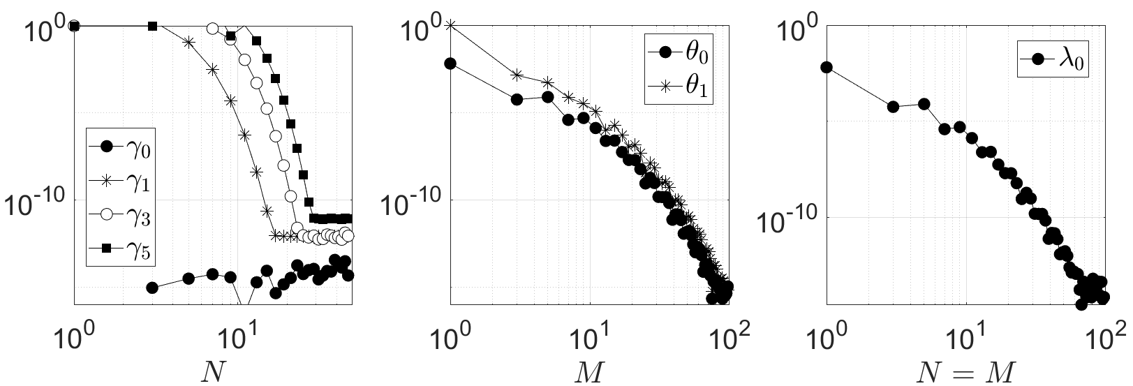
Figure 7.1: Example 1: computed spectra in the complex plane with $l=1$ and $d=1$ for $\mathcal{K}^{a}$ (left), $J^{x}$ (center) and $\mathcal{B}$ (right) with $N=M=100$.

Figure 7.2: Example 1: errors in computing $\gamma_{0},\gamma_{1},\gamma_{3},\gamma_{5}$ (left), $\theta_{0},\theta_{1}$ (center) and $\lambda_{0}$ (right) with $l=1$ and $d=1$ for increasing values of $N$ and $M$. The reference values $\gamma_{1}\approx-1.070249248997922+9.438599419667414i$, $\gamma_{3}\approx-2.772533303698945+21.842287295644464i$, $\gamma_{5}\approx-3.683984412603065+34.410428157635607i$ are obtained with $N=1000$; the reference values $\theta_{0}\approx 0.584294111974084$ and $\theta_{1}\approx 0.062556017866521$ are obtained with $M=1000$.

With these choices 2 holds, thus we compute the eigenvalues of $\mathcal{K}_{N}^{a}$ and $\mathcal{J}_{M}^{x}$ separately. We use $N=M$. Moreover, $\Pi_{0}(a)=1-a$ and, for $R=1$, $\gamma_{0}=0$. Finally, since $\beta$ is piecewise defined, we resort to the piecewise approach mentioned in remark 5.5.

Figure 7.3: Example 1: computed spectra of $\mathcal{B}$ in the complex plane with $l=1$, $d=1$ and $R=1.5$ (left), $R\approx 0.7277628676660066$ (center) and $R=0.1$ (right) with $N=M=100$.

Computed spectra are shown in fig. 7.2 for $l=1$ and $d=1$. For the same values, the convergence behavior is illustrated in fig. 7.2, which confirms corollary 5.2 and theorem 5.4 showing also how the error constants are affected by $|\gamma|$ and $|\theta|$.

Figure 7.4: Example 1: level curves for $\lambda_{0}$ as a function of $(d,l)$ and stability boundary (thick line) with $R=0.7$ and $N=M=30$.

With the proposed technique one can easily perform a bifurcation analysis of the null equilibrium with respect to $R$, fig. 7.3 with $l=1$ and $d=1$, finding a transcritical bifurcation at $R\approx 0.7277628676660066$ (correspondingly $\gamma_{0}\approx 0.415705888025916$). Level curves of $\lambda_{0}$ as a function of $(d,l)$ are reported in fig. 7.4. The principal eigenvalue is a decreasing function of $d$ and an increasing function of $l$, confirming the results in [19].

Example 2

We consider $a^{\dagger}=1$,

$$\beta(a,x)=\beta_{0}\chi_{\left[\frac{1}{2},\ a^{\dagger}\right]}(a)(2-x^{2}),\quad\mu_{0}(a)=\frac{1}{a^{\dagger}-a},\quad\mu_{1}(a,x)=\frac{1}{1+x^{2}}$$

and

$$J(x)=\pi^{-\frac{1}{2}}e^{-x^{2}}$$

with $\beta_{0}>0$.

Differently from section 7, $\beta$ and $\mu_{1}$ depend also on $x$. Yet, these choices satisfy the conditions of [19]. Again, we use the piecewise approach with $N=M$.

Figure 7.7 shows the computed spectrum of $\mathcal{B}$ (left) and the convergence diagram for the first two rightmost eigenvalues $\lambda_{0}$ and $\lambda_{1}$ (right) with $\beta_{0}=8$ and $d=l=1$. fig. 7.7 and fig. 7.7 show the computed eigenfunctions of $\mathcal{B}$ and $\mathcal{A}$, respectively, for $\lambda_{0}$ and $\lambda_{1}$. In fig. 7.7 (left) we observe the presence of a positive eigenfunction with a simple dominant real eigenvalue, i.e., $\lambda_{0}$ , whereas in fig. 7.7 (right) the eigenfunction of $\lambda_{1}$ changes sign. Note that in fig. 7.7 (left) the corresponding eigenfunction of $\mathcal{B}$ is increasing and vanishes only for $a=0$ as it is relevant to the age-integrated state, whereas in fig. 7.7 (right) the eigenfunction of $\lambda_{1}$ is not monotone. Accordingly to the theory of [19], this suggests that the proposed approach correctly approximates the principal eigenvalue $\lambda_{0}$. Eventually, fig. 7.10 shows the level curves of $\lambda_{0}$ as a function of $(d,l)$. As in Example 1, $\lambda_{0}$ is a decreasing function of $d$ and an increasing function of $l$, confirming again the results in [19].

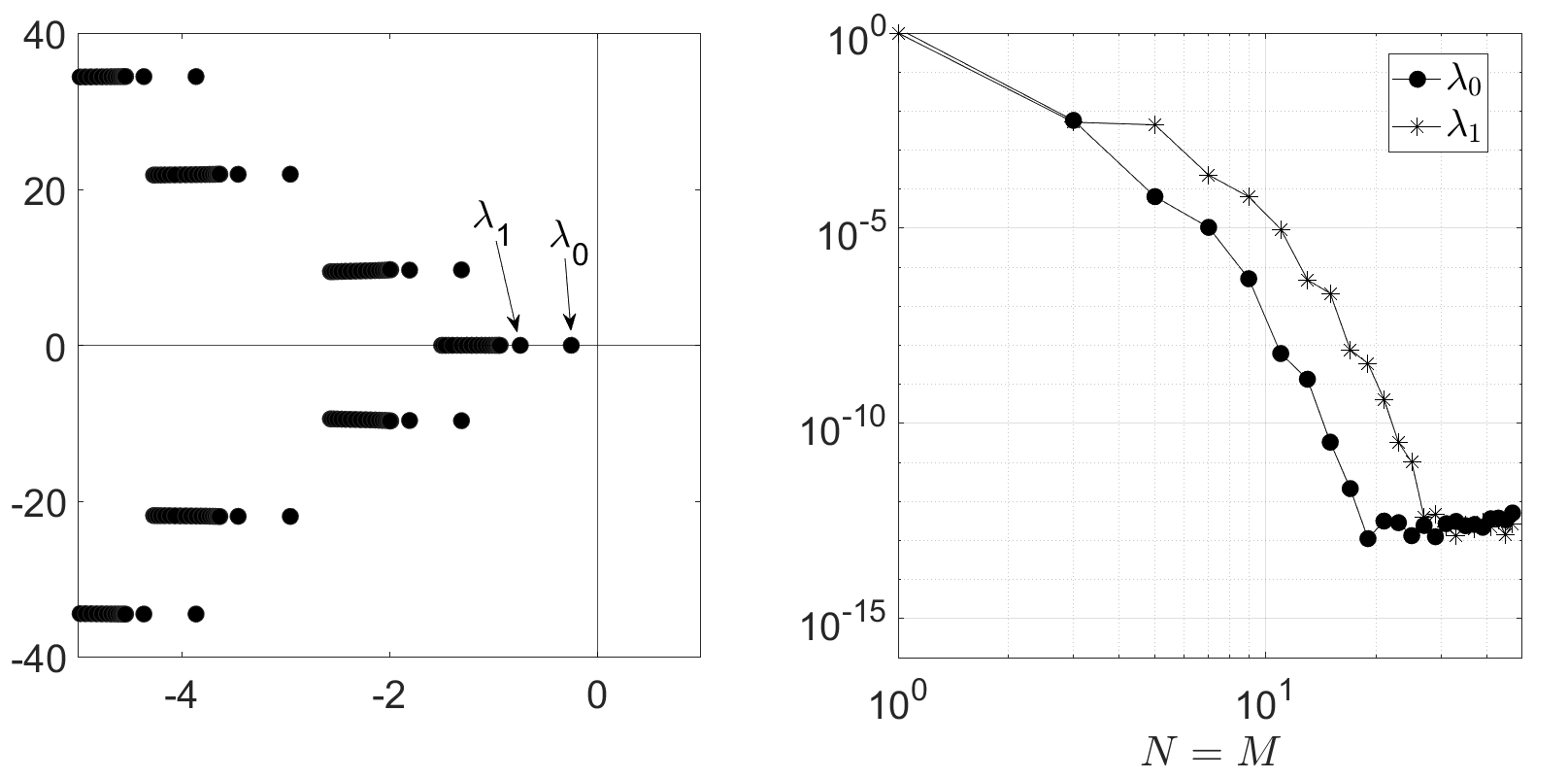
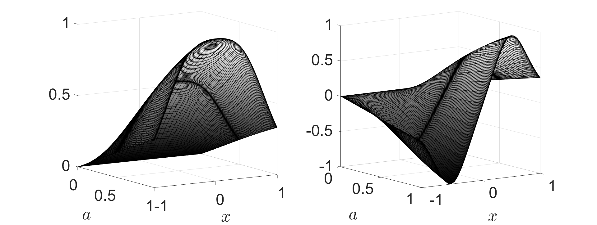
Figure 7.5: Example 2: spectrum of $\mathcal{B}$ in the complex plane computed with $N=M=50$ (left) and convergence diagram for the first two rightmost eigenvalues $\lambda_{0}$ and $\lambda_{1}$ (right) with $\beta_{0}=8$ and $d=l=1$. The reference values $\lambda_{0}\approx-0.248872934970194$ and $\lambda_{1}\approx-0.739612643296491$ are obtained with $N=M=100$.

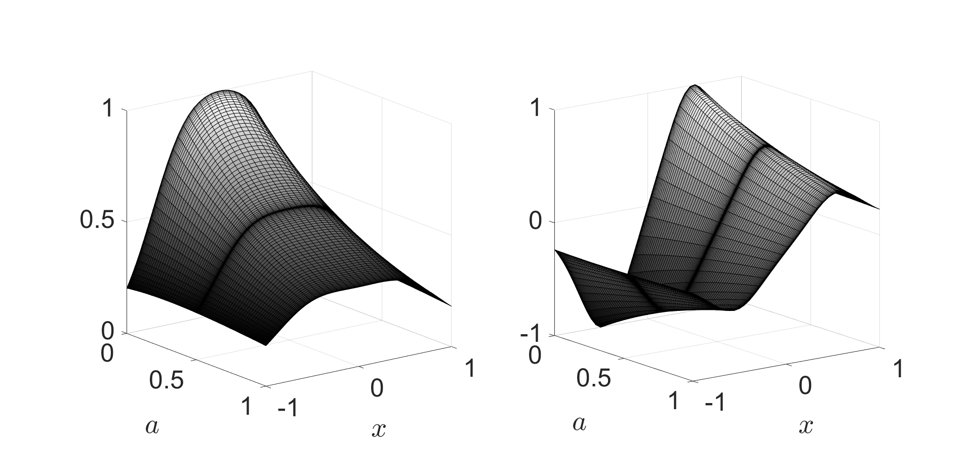
Figure 7.6: Example 2: computed eigenfunctions of $\mathcal{B}$ relevant to $\lambda_{0}$ (left) and $\lambda_{1}$ (right) with $\beta_{0}=8$, $d=l=1$ and $N=M=50$.

Figure 7.7: Example 2: computed eigenfunctions of $\mathcal{A}$ relevant to $\lambda_{0}$ (left) and $\lambda_{1}$ (right) with $\beta_{0}=8$, $d=l=1$ and $N=M=50$.

Example 3

We consider $a^{\dagger}=1$, $d=1$,

$$\beta(a,x)=\beta(a)=\beta_{0}\chi_{\left[\frac{1}{2},\ a^{\dagger}\right]}(a),\quad\mu_{0}(a)=\frac{1}{a^{\dagger}-a},\quad\mu_{1}(a,x)\equiv 0,$$

$$J(x)=\pi^{-1}e^{-\|x\|_{2}^{2}}$$

and $\Omega:=\{x\in\mathbb{R}^{2}\ |\ \|x\|_{2}<R\}$ for $R>0$. By using polar coordinates the diffusion operator $\tilde{\mathcal{J}^{x}}$ on $AC_{0}\left([0,a^{\dagger}],L^{2}([0,R]\times[0,2\pi],\mathbb{R})\right)$ reads

$$\tilde{\mathcal{J}^{x}}\tilde{\psi}(a,r,\theta)=\int_{0}^{R}\int_{0}^{2\pi}J(r\cos\theta-\rho\cos\varphi,r\sin\theta-\rho\sin\varphi)\tilde{\psi}(a,\rho,\varphi)\rho\mathop{}\!\mathrm{d}\varphi\mathop{}\!\mathrm{d}\rho.$$

Observe that with these choices 2 holds. Again, we use the piecewise approach with $N=M$ (note that, being $\Omega\subset\mathbb{R}^{2}$, here $M$ represents the degree of the univariate polynomials in both directions of the tensorial approach). Figure 7.10 shows the computed spectrum of $\mathcal{B}$ (left) and the convergence diagram for the first two rightmost eigenvalues $\lambda_{0}$ and $\lambda_{1}$ (right) with $\beta_{0}=8$ and $R=1$. Figure 7.10 shows the level curves of $\lambda_{0}$ as a function of $(d,l)$, which again confirm the results of [19].

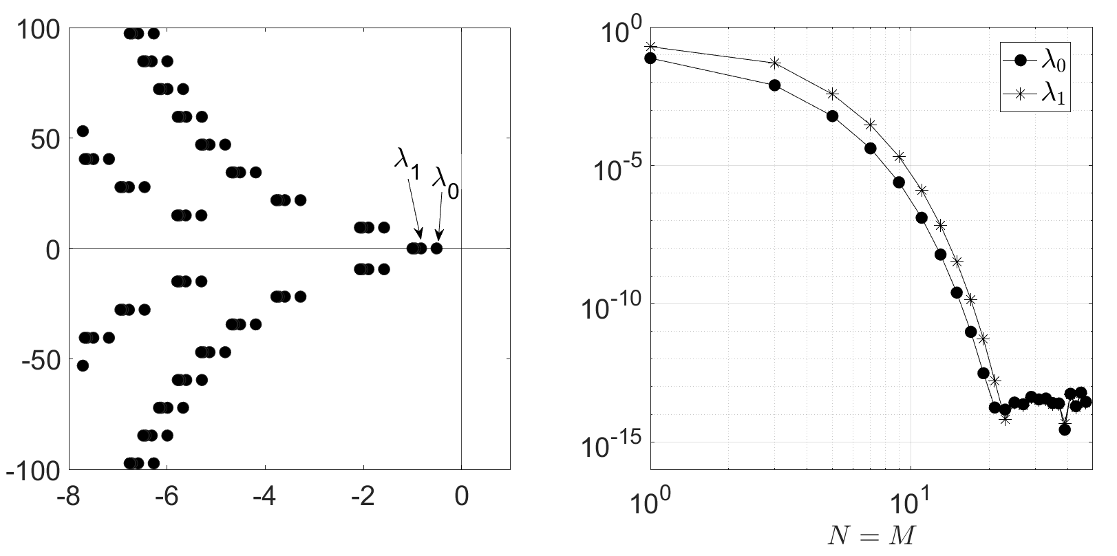
Figure 7.8: Example 2: level curves for $\lambda_{0}$ as a function of $(d,l)$ and stability boundary (thick line) with $\beta_{0}=10$ and $N=M=30$.

Figure 7.9: Example 3: spectrum of $\mathcal{B}$ in the complex plane computed with $N=M=50$ (left) and convergence diagram for the first two rightmost eigenvalues $\lambda_{0}$ and $\lambda_{1}$ (right) with $\beta_{0}=8$, $d=R=1$. The reference values $\lambda_{0}\approx-0.508459905995625$ and $\lambda_{1}\approx-0.827016421828640$ are obtained with $N=M=100$.

Figure 7.10: Example 3: level curves of $\lambda_{0}$ as a function of $(d,R)$ and stability boundary (thick line) with $\beta_{0}=10$ and $N=M=30$.

8 Nonlocal diffusion of Neumann type

Now we briefly consider models with nonlocal diffusion of Neumann type, i.e., models in which the diffusion is limited to a certain region $\Omega\subset\mathbb{R}^{n}$ [30]. The prototype model is

$$\left\{\begin{array}[]{rlll}\mathcal{D}u(t,a,x)&=&d\displaystyle\int_{\Omega}J(x-y)[u(t,a,y)\\[5.69054pt] &&-u(t,a,x)]\mathop{}\!\mathrm{d}y&\\[8.53581pt] &&-\mu(a,x)u(t,a,x),&t>0,\ a\in[0,a^{\dagger}],\ x\in\Omega,\\[5.69054pt] u(t,0,x)&=&\displaystyle\int_{0}^{a^{\dagger}}\beta(\hat{a},x)u(t,\hat{a},x)\mathop{}\!\mathrm{d}\hat{a},&t>0,\ x\in\Omega,\\[8.53581pt] u(0,a,x)&=&u_{0}(a,x),&a\in[0,a^{\dagger}],\ x\in\Omega,\end{array}\right.$$ (8.1)

where $\mathcal{D}$ is defined as in (2.2). Again, the semigroup generated by (8.1) is not eventually compact in general, yet stability is still governed by the spectral abscissa $s(\mathcal{A})$ of the relevant infinitesimal generator $\mathcal{A}$ (which can be derived as in section 3). Moreover, $s(\mathcal{A})$ can be shown to be its principal eigenvalue under suitable assumptions [30].

By replacing $\mathcal{J}-\mathcal{I}_{U}$ with $\mathcal{J}-\mathcal{C}$ for $\mathcal{C}\colon U\to U$ defined as

$$\mathcal{C}\phi(a,x):=\phi(a,x)\int_{\Omega}J(x-y)\mathop{}\!\mathrm{d}y$$

and by proceeding as in sections 3 and 4, we can reformulate (8.1) by integration of the age-state and derive a similar numerical approximation for the spectrum of the infinitesimal generator.

Anyway, let us remark that a decomposition as in theorem 3.2 has not been proved to hold true for the case of Neumann diffusion, although it is easy to see that

$$\sigma_{p}(\mathcal{K}^{a})+\sigma_{p}(\mathcal{J}^{x}-\mathcal{C}^{x})\subseteq\sigma_{p}(\mathcal{B}),$$

where $\mathcal{C}^{x}\colon L^{2}(\Omega,\mathbb{R})\to L^{2}(\Omega,\mathbb{R})$ is defined as

$$\mathcal{C}^{x}g(x):=g(x)\int_{\Omega}J(x-y)\mathop{}\!\mathrm{d}y.$$

Nevertheless, in [30, Theorem 4.1] it is proved that if $\lambda_{0}\in\sigma_{p}(\mathcal{A})$ is associated with a positive eigenfunction $\phi$, then $\lambda_{0}$ is the principal eigenvalue of $\mathcal{A}$. Holding this true, we can still characterize the principal eigenvalue of $\mathcal{B}$ under 2. In fact the Neumann eigenvalue problem

$$-(\mathcal{J}^{x}-\mathcal{C}^{x})g(x)=\theta g(x)$$

has principal eigenvalue $\theta_{0}=0$ with $g_{0}$ constant [37]. Thus $s(\mathcal{B})=\lambda_{0}=\gamma_{0}-\theta_{0}=\gamma_{0}$ with associated eigenfunction $\psi(a,x)=f_{0}(a)$, where $f_{0}$ is the eigenfunction for $\mathcal{K}^{a}$ relevant to the principal eigenvalue $\gamma_{0}$. Finally, a decomposition like (4.4) holds for the discretized problem.

In light of the above results, we can proceed as in section 5 to prove that, under 2, the eigenvalues of $\mathcal{B}_{N,M}$ converge to those of $\mathcal{B}$ (in particular $\lambda_{0}$ is approximated by a converging sequence of eigenvalues). The proof again consists in considering the separated eigenvalue problems for $\mathcal{K}_{N}^{a}$ and $\mathcal{J}_{M}^{x}-\mathcal{C}_{M}^{x}$. While the convergence analysis relevant to $\mathcal{K}_{N}^{a}$ remains unchanged, a slight modification is required for the space counterpart. Indeed, $\mathcal{J}^{x}-\mathcal{C}^{x}$ is not compact in general, but being bounded and self-adjoint, theorem 5.1 and corollary 5.2 remain valid thanks to the strong stabilty guaranteed by a (Galerkin-type) spectral projection method as the one presented in section 4 [16, Section 4].

As a numerical test, we consider the same coefficients of Example 1 in section 7, thus ensuring 2. Figure 8.1 shows the computed spectrum of $\mathcal{B}$ (left, recall that $\gamma_{0}=0$) and the convergence diagram for $\lambda_{0}$ and $\lambda_{1}$. The error for $\lambda_{0}$ is at the machine precision already for small values of $N=M$ while the error for $\lambda_{1}$ decreases with infinite order (observe that the relevant eigenfunction is of class $C^{\infty}$).

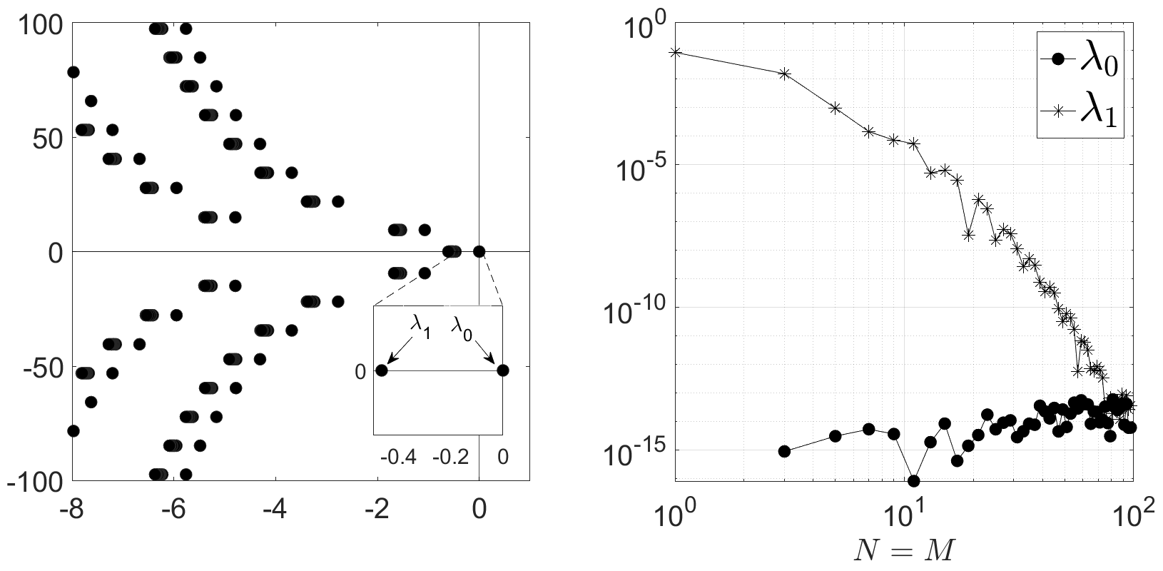
Figure 8.1: Nonlocal diffusion of Neumann type: spectrum of $\mathcal{B}$ in the complex plane computed with $N=M=100$ (left) and convergence diagram for the first two rightmost eigenvalues $\lambda_{0}$ and $\lambda_{1}$ (right) with $d=l=1$. The reference value $\lambda_{1}\approx-0.467278026690667$ is obtained with $N=M=1000$.

9 Conclusions

In this work we proposed a numerical approach to approximate the spectrum of the infinitesimal generator of the semigroup associated to an age-structured model with nonlocal diffusion of Dirichlet or Neumann type and proved the convergence of the approximated eigenvalues in the case of separable model coefficients (2).

Numerical results suggest that the proposed numerical scheme is able to approximate the principal eigenvalue also in the case of parameters dependent on the spatial variable. Future work will investigate the convergence of the method in this general case and also with regards to the monotonicity of the approximation with respect to the discretization parameters (which we did not observe in general but could be a desirable property under additional hypotheses). It is also interest of the authors to tackle the problem of the numerical approximation of $R_{0}$ in age-structured epidemic models involving nonlocal diffusion and also additional structuring variables [5, 8, 10, 28, 31]. Another direction could be investigating the stability of models on unbounded spatial domains [38].

References

• [1] A. Andò, S. De Reggi, D. Liessi and F. Scarabel “A pseudospectral method for investigating the stability of linear population models with two physiological structures” In Math. Biosci. Eng. 20.3, 2023, pp. 4493–4515 DOI: 10.3934/mbe.2023208
• [2] P. Auger, P. Magal and S. Ruan “Structured population models in biology and epidemiology” Springer, 2008
• [3] P. W. Bates and G. Zhao “Existence, uniqueness and stability of the stationary solution to a nonlocal evolution equation arising in population dispersal” In J. Math. Anal. 332.1 Elsevier, 2007, pp. 428–440 DOI: https://doi.org/10.1016/j.jmaa.2006.09.007
• [4] D. Breda et al. “Stability analysis of age-structured population equations by pseudospectral differencing methods” In J. Math. Biol. 54.5 Springer, 2007, pp. 701–720 DOI: https://doi.org/10.1007/s00285-006-0064-4
• [5] D. Breda et al. “Bivariate collocation for computing $R_{0}$ in epidemic models with two structures” In Comput. Math. with Appl. Elsevier, 2021 DOI: https://doi.org/10.1016/j.camwa.2021.10.026
• [6] D. Breda et al. “Numerical bifurcation analysis of physiologically structured population models via pseudospectral approximation” In Vietnam J. Math. 49.1 Springer, 2021, pp. 37–67 DOI: https://doi.org/10.1007/s10013-020-00421-3
• [7] D. Breda, O. Diekmann, S. Maset and R. Vermiglio “A numerical approach for investigating the stability of equilibria for structured population models” In J. Biol. Dyn. 7.sup1 Taylor & Francis, 2013, pp. 4–20 DOI: https://doi.org/10.1080/17513758.2013.789562
• [8] D. Breda, F. Florian, J. Ripoll and R. Vermiglio “Efficient numerical computation of the basic reproduction number for structured populations” In J. Comput. Appl. Math 384 Elsevier, 2021, pp. 113165 DOI: https://doi.org/10.1016/j.cam.2020.113165
• [9] D. Breda, M. Iannelli, S. Maset and R. Vermiglio “Stability analysis of the Gurtin–MacCamy model” In SIAM J. Numer. Anal. 46.2 SIAM, 2008, pp. 980–995 DOI: https://doi.org/10.1137/070685658
• [10] D. Breda, T. Kuniya, J. Ripoll and R. Vermiglio “Collocation of next-generation operators for computing the basic reproduction number of structured populations” In J. Sci. Comput. 85.2 Springer, 2020, pp. 1–33 DOI: https://doi.org/10.1007/s10915-020-01339-1
• [11] D. Breda, S. Maset and R. Vermiglio “Pseudospectral approximation of eigenvalues of derivative operators with non-local boundary conditions” In Appl. Numer. Math. 56.3-4 Elsevier, 2006, pp. 318–331 DOI: https://doi.org/10.1016/j.apnum.2005.04.011
• [12] D. Breda, S. Maset and R. Vermiglio “Approximation of eigenvalues of evolution operators for linear retarded functional differential equations” In SIAM J. Numer. Anal. 50.3 SIAM, 2012, pp. 1456–1483 DOI: https://doi.org/10.1137/100815505
• [13] D. Breda, S. Maset and R. Vermiglio “Computing the eigenvalues of Gurtin–MacCamy models with diffusion” In IMA J. Numer. Anal. 32.3 Oxford University Press, 2012, pp. 1030–1050 DOI: https://doi.org/10.1093/imanum/drr004
• [14] H. Brezis “Functional analysis, Sobolev spaces and partial differential equations” Springer, 2011
• [15] C. Canuto, M.Y. Hussaini, A. Quarteroni and T.A. Zang “Spectral methods in fluid dynamics” Springer-Verlag, 1988
• [16] F. Chatelin “Spectral approximation of linear operators” SIAM, 2011
• [17] C. Cusulin “Diffusion and age in population dynamics”, 2006
• [18] O. Diekmann, F. Scarabel and R. Vermiglio “Pseudospectral discretization of delay differential equations in sun-star formulation: Results and conjectures” In Discrete Cont. Dyn.-S 13.9 DiscreteContinuous Dynamical Systems-S, 2020, pp. 2575–2602 DOI: https://doi.org/10.3934/dcdss.2020196
• [19] A. Ducrot, H. Kang and S. Ruan “Age-structured Models with Nonlocal Diffusion of Dirichlet Type, $I$: Principal Spectral Theory and Limiting Properties”, 2022 eprint: 2205.09642
• [20] K.J. Engel, R. Nagel and S. Brendle “One-parameter semigroups for linear evolution equations” Springer, 2000
• [21] P. Erdos and P. Turán “On interpolation I” In Ann. Math. JSTOR, 1937, pp. 142–155 DOI: https://doi.org/10.2307/1968516
• [22] J. García-Melián and J. D. Rossi “On the principal eigenvalue of some nonlocal diffusion problems” In J. Differ. Equ. 246.1 Elsevier, 2009, pp. 21–38 DOI: https://doi.org/10.1016/j.jde.2008.04.015
• [23] G. Gripenberg, S.-O. Londen and O. Staffans “Volterra integral and functional equations” Cambridge University Press, 1990
• [24] R. A. Horn and C. R. Johnson “Topics in matrix analysis, 1991” In Cambridge University Presss, Cambridge 37, 1991, pp. 39
• [25] M. Iannelli “Mathematical theory of age-structured population dynamics” In Giardini editori e stampatori in Pisa, 1995
• [26] H. Inaba “Age-structured population dynamics in demography and epidemiology” Springer, 2017
• [27] H. Kang and S. Ruan “Approximation of random diffusion by nonlocal diffusion in age-structured models” In Z. Angew. Math. Phys. 72.3 Springer, 2021, pp. 1–17 DOI: https://doi.org/10.1007/s00033-021-01538-2
• [28] H. Kang and S. Ruan “Mathematical analysis on an age-structured SIS epidemic model with nonlocal diffusion” In J. Math. Biol. 83.1 Springer, 2021, pp. 5 DOI: https://doi.org/10.1007/s00285-021-01634-x
• [29] H. Kang and S. Ruan “Nonlinear age-structured population models with nonlocal diffusion and nonlocal boundary conditions” In J. Differ. Equ. 278 Elsevier, 2021, pp. 430–462 DOI: https://doi.org/10.1016/j.jde.2021.01.004
• [30] H. Kang and S. Ruan “Principal spectral theory and asynchronous exponential growth for age-structured models with nonlocal diffusion of Neumann type” In Math. Ann. 384.1 Springer, 2022, pp. 1–49 DOI: https://doi.org/10.1007/s00208-021-02270-y
• [31] H. Kang, S. Ruan and X. Yu “Age-structured population dynamics with nonlocal diffusion” In J. Dyn. Diff. Equat. Springer, 2020, pp. 1–35 DOI: https://doi.org/10.1007/s10884-020-09860-5
• [32] C.Y. Kao, Y. Lou and W. Shen “Random dispersal vs. non-local dispersal” In Discrete. Contin. Dyn. Syst. Ser. A 26.2 American Institute of Mathematical Sciences, 2010, pp. 551 DOI: https://doi.org/10.3934/dcds.2010.26.551
• [33] R. Kress, V. Maz’ya and V. Kozlov “Linear integral equations” Springer, 1989
• [34] T. Kuniya and J. Wang “Global dynamics of an SIR epidemic model with nonlocal diffusion” In Nonlinear Anal. Real World Appl. 43 Elsevier, 2018, pp. 262–282 DOI: https://doi.org/10.1016/j.nonrwa.2018.03.001
• [35] L. Liu and P. Weng “A nonlocal diffusion model of a single species with age structure” In J. Math. Anal. 432.1 Elsevier, 2015, pp. 38–52 DOI: https://doi.org/10.1016/j.jmaa.2015.06.052
• [36] T. J. Rivlin “An introduction to the approximation of functions” Courier Corporation, 1981
• [37] J. D. Rossi “The First Eigenvalue for Nonlocal Operators” In Operator and Norm Inequalities and Related Topics Springer, 2022, pp. 741–772 DOI: https://doi.org/10.1007/978-3-031-02104-6_22
• [38] S. Ruan “Spatial-temporal dynamics in nonlocal epidemiological models” In Mathematics for life science and medicine Springer, 2007, pp. 97–122 DOI: https://doi.org/10.1007/978-3-540-34426-1_5
• [39] L. N. Trefethen “Is Gauss quadrature better than Clenshaw–Curtis?” In SIAM Rev. 50.1 SIAM, 2008, pp. 67–87 DOI: https://doi.org/10.1137/060659831
• [40] G. F. Webb “An operator-theoretic formulation of asynchronous exponential growth” In Trans. Am. Math. Soc. 303.2, 1987, pp. 751–763 DOI: https://doi.org/10.2307/2000695
• [41] W.B. Xu, W.T. Li and S. Ruan “Spatial propagation in nonlocal dispersal Fisher-KPP equations” In J. Funct. Anal. 280.10 Elsevier, 2021, pp. 108957 DOI: https://doi.org/10.1016/j.jfa.2021.108957
• [42] F.Y. Yang, W.T. Li and S. Ruan “Dynamics of a nonlocal dispersal SIS epidemic model with Neumann boundary conditions” In J. Differ. Equ. 267.3 Elsevier, 2019, pp. 2011–2051 DOI: https://doi.org/10.1016/j.jde.2019.03.001
• [43] G. Zhao and S. Ruan “Spatial and temporal dynamics of a nonlocal viral infection model” In SIAM J. Appl. Math. 78.4 SIAM, 2018, pp. 1954–1980 DOI: https://doi.org/10.1137/17M1144106