The D4/D8 model and holographic QCD

Abstract

As a top-down holographic approach, the D4/D8 model is expected to be the holographic version of QCD since it almost includes all the elementary features of QCD based on string theory. In this manuscript, we review the fundamental properties of the D4/D8 model with respect to the D4-brane background, embedding of flavor branes and holographic quark, gluon, meson, baryon and glueball with various symmetries, then we also take a look at some interesting applications and developments based on this model.

Keywords: Gauge-gravity duality; AdS/CFT correspondence; Holographic QCD

^∗Si-wen Li, ^†Xiao-tong Zhang,

1 Introduction

Although it has been about 25 years since the proposal of AdS/CFT and gauge-gravity duality with holography [1, 2, 3], it remains to attract great interests today. The most significant part of AdS/CFT and gauge-gravity duality is that people can evaluate strongly coupled quantum field theory (QFT) by analyzing quantitatively its associated gravity theory in the weak coupling region. So it provides a holographic way to study the strongly coupled QFT in which traditional QFT based on perturbation method is out of reach. Accordingly, a large number of publications about strongly coupled QFT through AdS/CFT and gauge-gravity duality have appeared, for example on Wilson loop and quark potential [4, 5, 6], transport coefficient [7, 8, 9], fermionic correlation function [10, 11], the Schwinger effect [12], quantum entanglement entropy [13, 14] and quantum information on black hole [15] which have become most remarkable works in this field.

On the other hand, QCD (quantum chromodynamics) as the fundamental theory describing the property of strong interaction is extremely complex in the strong coupling region, especially at finite temperature with dense matter due to its asymptotic freedom [16, 17], hence the holographic version of QCD is natural to become an interesting topic. While there are several models and theories attempting to give a holographic version of QCD (e.g. bottom-up approaches [18, 19, 20], D3/D7 approach [21], D4/D6 approach [22]), one of the most successful achievements in holography is the D4/D8 model (also named as Witten-Sakai-Sugimoto model) [23, 24, 25] which includes almost all the elementary features of QCD in a very simple way, e.g. meson, baryon [26, 27, 28], glueball [29, 30, 31, 32], deconfinement transition [33, 34, 35], chiral phase [36, 37], heavy flavor [38, 39, 40], $\theta$ term and QCD axion [41, 42, 43, 44, 45], nucleon interaction [46, 47, 48, 49, 50, 51, 52]. The D4/D8 model is based on the holographic duality between the 11-dimensional (11d) M-theory on $\mathrm{AdS_{7}}\times S^{4}$ and the $\mathcal{N}=\left(2,0\right)$ super conformal field theory (SCFT) on $N_{c}$ M5-branes [53]. By using the dimensional reduction in [23, 54], it reduces to the correspondence of the pure Yang-Mills theory on $N_{c}$ D4-branes compactified on a circle and 10d IIA supergravity (SUGRA). Flavors as $N_{f}$ pairs of D8- and anti D8-branes ($\mathrm{D8/\overline{D8}}$) can be further introduced into the geometric background produced by the $N_{c}$ D4-branes, so the dual theory includes flavored fundamental quarks which would be more close to the realistic QCD. Beside, as the D4/D8 model is a T-dualized version of D3/D9 system [55], the fundamental quark and meson in the D4/D8 model can therefore be identified to the $4-8$ and $8-8$ strings respectively by following the same discussion in D3/D9 system [55]. Moreover, the baryon vertex is identified as a D4-brane wrapped on $S^{4}$ [26] and the glueball is recognized to be the bulk gravitational polarization [29, 30]. The chiral phase is determined by the embedding configuration of the $\mathrm{D8/\overline{D8}}$-branes due to the gauge symmetry on their worldvolume [56] while the deconfinement transition is suggested to be the Hawking-Page transition in this model [33, 34, 35, 36]. Altogether, this model includes all the fundamental elements of QCD thus can be treated as a holographic version of QCD.

In this review, we will revisit the above properties of the D4/D8 model, then take a brief look at some recently relevant developments and holographic approaches with this model. The outline of this review is as follows. In Section 2, we will review the relation of 11d M-theory and IIA SUGRA with respect to the case of M5-brane and D4-brane. Afterwards, it is the embedding configuration of the $\mathrm{D8/\overline{D8}}$-branes to the D4-brane background, the holographic quark, gluon, meson, baryon and glueball with various symmetries which are all the relevant objects in hadron physics. In Section 3, we review several topics about the developments and holographic approaches of this model which includes deconfinement transition, chiral transition, Higgs mechanism and heavy-light meson or baryon, interaction involving glueball and QCD $\theta$ term in holography. In the appendix, we give the general form of the black brane solution in type II SUGRA, the relevant dimensional reduction for spinor and discussion about supersymmetric meson which are useful to the main content of this paper.

2 The D4/D8 model

In this section, we will revisit the D4-brane background and the embedding of the probe $\mathrm{D8/\overline{D8}}$-branes. Then we will review how to identify quarks, gluon, meson, baryon and glueball with various symmetries in this model.

2.1 11d supergravity and D4-brane background

The D4-brane background of the D4/D8 model is based on the holographic duality between the type $\mathcal{N}=\left(2,0\right)$ super conformal field theory (SCFT) on coincident $N_{c}$ M5-branes and 11-dimensional (11d) M-theory on $\mathrm{AdS}_{7}\times S^{4}$ [53]. In order to obtain a geometric solution, the effective action of the M-theory is necessary which is known as the 11d supergravity action. In the large-$N_{c}$ limit, the geometric background can be obtained by solving its bosonic part which is consisted of metric (elfbein) and a three-from $C_{3}$ as [57],

$$S_{\mathrm{SUGRA}}^{11\mathrm{d}}=\frac{1}{2\kappa_{11}^{2}}\int d^{11}x\sqrt{-g}\left[\mathcal{R}^{(11)}-\frac{1}{2}\left|F_{4}\right|^{2}\right]-\frac{1}{12\kappa_{11}^{2}}\int C_{3}\wedge F_{4}\wedge F_{4},$$ (2.1)

where $F_{4}=dC_{3}$. The convention in (2.1) is as follows. $\mathcal{R}^{(11)}$ refers to the 11d scalar curvature, $\kappa_{11}$ is the 11d gravity coupling constant given by,

$$2\kappa_{11}^{2}=16\pi G_{11}=\frac{1}{2\pi}\left(2\pi l_{p}\right)^{9},$$ (2.2)

where $G_{11}$ is 11d Newton’s constant, $l_{p}$ is the Planck length. The quantity $\left|F_{4}\right|^{2}$ can be obtained by a general notation of an $n$-form $F_{n}$ as,

$$\left|F_{n}\right|^{2}=\frac{1}{n!}g^{A_{1}B_{1}}g^{A_{2}B_{2}}...g^{A_{n}B_{n}}F_{A_{1}A_{2}...A_{n}}F_{B_{1}B_{2}...B_{n}},$$ (2.3)

where $g_{AB}$ refers to the metric on the manifold. We note that in (2.1) the last term is a Chern-Simons structure which is independent on the metric or elfbein while the first term depends on the metric or elfbein through the metric combination

$$g_{AB}=e_{A}^{a}\eta_{ab}e_{B}^{b}.$$ (2.4)

The solution for extremal coincident $N_{c}$ M5-branes is obtained as,

$$ds_{\mathrm{11d}}^{2}= H_{5}\left(r\right)^{-\frac{1}{3}}\eta_{MN}dx^{M}dx^{N}+H_{5}\left(r\right)^{\frac{2}{3}}\left(dr^{2}+r^{2}d\Omega_{4}^{2}\right),$$

$$H_{5}\left(r\right)= 1+\frac{r_{5}^{3}}{r^{3}},\ \left({}^{*}F_{4}\right)_{r012...5}=-\frac{3r_{5}^{3}}{r^{4}H_{5}^{2}},$$ (2.5)

where $r$ denotes the radial coordinate to the M5-branes and $M,N$ run over the M5-branes. Using the BPS condition for M5-brane,

$$2\kappa_{11}^{2}T_{\mathrm{M5}}N_{c}=\int_{S^{4}}F_{4},$$ (2.6)

it leads to

$$r_{5}^{3}=\pi N_{c}l_{p}^{3},$$ (2.7)

where $T_{\mathrm{M5}}=\frac{1}{\left(2\pi\right)^{5}l_{p}^{6}}$ refers to the tension of the M5-brane. Taking the near horizon limit $H_{5}\rightarrow\frac{r_{5}^{3}}{r^{3}}$ and replacing the variables as

$$\left\{r,r_{5},x^{i},\Omega_{4}\right\}\rightarrow\left\{r^{2},\frac{L}{2},\frac{1}{\sqrt{L}}x^{i},\frac{1}{\sqrt{L}}\Omega_{4}\right\},$$ (2.8)

the metric presented in (2.5) reduces to,

$$ds_{\mathrm{11d}}^{2}=\frac{r^{2}}{L^{2}}\eta_{MN}dx^{M}dx^{N}+\frac{L^{2}}{r^{2}}\left(dr^{2}+\frac{r^{2}}{4}d\Omega_{4}^{2}\right),$$ (2.9)

describing the standard form of $\mathrm{AdS}_{7}\times S^{4}$ where the radius of $S^{4}$ is $L/2$. In addition, the action (2.1) also allows the near-extremal M5-brane solution which, after taking near horizon limit and replacement (2.8), is

$$ds_{\mathrm{11d}}^{2} =\frac{r^{2}}{L^{2}}\left[-f\left(r\right)\left(dx^{0}\right)^{2}+\sum_{i=1}^{5}dx^{i}dx^{i}\right]+\frac{L^{2}}{r^{2}}\left[\frac{dr^{2}}{f\left(r\right)}+\frac{r^{2}}{4}d\Omega_{4}^{2}\right],$$

$$f\left(r\right) =1-\frac{r_{H}^{6}}{r^{6}},$$ (2.10)

The constant $r_{H}$ refers to the location of the horizon which can be determined by omitting the conical singularity as,

$$\beta_{T}=\frac{2\pi L^{2}}{3r_{H}},$$ (2.11)

where $\beta_{T}$ is the size of the compactified direction $x^{0}$.

In order to obtain a QCD-like low-energy theory in holography, Witten proposed a scheme in [23] based on the above M5-brane solution. Specifically, the first step is to campactify one spacial direction (denoted by $x^{5}$) of M5-branes on a circle with periodic condition for fermions, which means the supersymmetry remains. Accordingly the resultant theory is a supersymmetric gauge theory above the size of the circle. Then, recall the relation between M-theory and IIA string theory, the 11d metric presented in (2.9) or (2.10) reduces to a 10d metric as,

$$ds_{\mathrm{11d}}^{2}=e^{-\frac{2}{3}\phi}ds_{\mathrm{10d}}^{2}+e^{\frac{4}{3}\phi}\left(dx^{5}\right)^{2},$$ (2.12)

with the non-trivial dilaton $e^{\phi}=\left(r/L\right)^{3/2}$. For the later use, let us introduce another radial coordinates $U\in\left[U_{H},\infty\right)$ by

$$U=\frac{r^{2}}{2L},L=2R.$$ (2.13)

So in the large $N_{c}$ limit, the 11th direction $x^{5}$ presented in (2.12) vanishes due to (2.7) (2.8), which means the coincident $N_{c}$ M5-branes corresponds to coincident $N_{c}$ D4-branes for $N_{c}\rightarrow\infty$. And the remained 10d metric in (2.12) becomes the near-extremal black D4-brane solution as,

$$ds_{\mathrm{10d}}^{2} =\left(\frac{U}{R}\right)^{3/2}\left[-f_{T}\left(U\right)\left(dx^{0}\right)^{2}+\sum_{i=1}^{4}dx^{i}dx^{i}\right]+\left(\frac{R}{U}\right)^{3/2}\left[\frac{dU^{2}}{f_{T}\left(U\right)}+U^{2}d\Omega_{4}^{2}\right],$$

$$f_{T}\left(U\right) =1-\frac{U_{H}^{3}}{U^{3}},F_{4}=3R^{3}g_{s}^{-1}\epsilon_{4},e^{\phi}=\left(\frac{U}{R}\right)^{3/4},R^{3}=\pi g_{s}N_{c}l_{s}^{3}$$ (2.14)

where $\epsilon_{4}$ refers to the volume form of a unit $S^{4}$. Once the formula (2.12) is imposed to action (2.1), the 11d SUGRA action reduces to the 10d type IIA SUGRA action exactly which is given as,,

$$S_{\mathrm{IIA}}^{10\mathrm{d}}=\frac{1}{2\kappa_{10}^{2}}\int d^{10}x\sqrt{-G}e^{-2\phi}\left[\mathcal{R}^{(10)}+4\partial_{\mu}\phi\partial\phi\right]-\frac{1}{4\kappa_{10}^{2}}\int d^{10}x\sqrt{-G}\left|F_{4}\right|^{2},$$ (2.15)

where $2\kappa_{10}^{2}=16\pi G_{10}=\left(2\pi\right)^{7}l_{s}^{8}g_{s}^{2}$ is the 10d gravity coupling constant. And it would be straightforward to verify that the solution (2.14) satisfies the equation of motion obtained by varying action (2.15).

The next step is to perform the double Wick rotation $\left\{x^{0}\rightarrow-ix^{4},x^{4}\rightarrow-ix^{0}\right\}$ on the metric (2.14) leading to a bubble D4-brane solution as,

$$ds_{\mathrm{10d}}^{2} =\left(\frac{U}{R}\right)^{3/2}\left[\eta_{\mu\nu}dx^{\mu}dx^{\nu}+f\left(U\right)\left(dx^{4}\right)^{2}\right]+\left(\frac{R}{U}\right)^{3/2}\left[\frac{dU^{2}}{f\left(U\right)}+U^{2}d\Omega_{4}^{2}\right],$$

$$f\left(U\right) =1-\frac{U_{KK}^{3}}{U^{3}},$$ (2.16)

which is defined only for $U\in\left[U_{KK},\infty\right)$. We have renamed $U_{H}$ as $U_{KK}$ in (2.16) since there is not a horizon in the bubble solution as it is illustrated in Figure 1 .

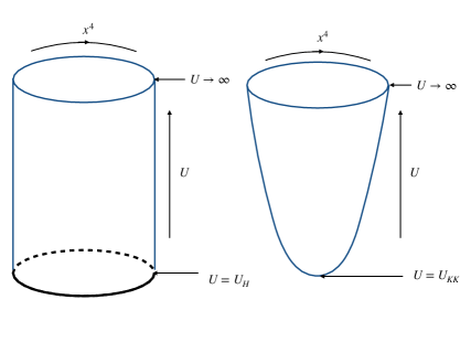
Figure 1: The compactified D4-brane geometry on $U-x^{4}$ plane. Left: The black D4-brane background geometry. Right: The D4 bubble geometry.

Now the direction of $x^{4}$ is periodic as,

$$x^{4}\sim x^{4}+\delta x^{4},\delta x^{4}=\frac{2\pi}{M_{KK}}=\frac{4\pi R^{3/2}}{3U_{KK}^{1/2}},$$ (2.17)

because it is identified as the time direction in the black brane solution (2.14). $M_{KK}$ refers to the Klein-Kaluza (KK) energy scale and the supersymmetry on the D4-branes breaks down below $M_{KK}$ by imposing the anti-periodic condition to the supersymmetric fermions along $x^{4}$. Accordingly, the low-energy zero modes on the D4-branes are the massless gauge field on the D4-branes and the scalar fields as the transverse modes of the D4-branes. While the scalar fields acquire mass via one-loop corrections, the trace part of the scalars $\phi^{i}$ and gauge field along $x^{4}$ direction $a_{4}$ remain to be massless. As they give irrelevant coupling terms in the low-energy effective theory on the D4-branes, it means the dual theory below $M_{KK}$ only contains 4d pure Yang-Mills gauge field as it is expected. Note that the three-from $C_{3}$ in 11d SUGRA (2.1) corresponds to the Ramond-Ramond (R-R) three-form in the type IIA string theory.

Besides, as the wrap factor $\left(U/R\right)^{3/2}$ in (2.16) never goes to zero, the dual theory would be able to exhibit confinement according to the behavior of the Wilson loop in this geometry. Since the solution (2.16) allows an arbitrarily large period for $x^{0}$, it implies the dual theory on the D4-brane could be defined at zero (or very low) temperature. Furthermore, in order to obtain a deconfined version of holographic QCD based on (2.16) at finite temperature, it is also possible to compactify one spacial direction (denoted by $x^{4}$) of the D4-branes in the background (2.14) with the anti-periodic condition for the supersymmetric fermions as it is displayed in (2.17) and Figure 1. In this case, the Hawking temperature $T$ in compactified background (2.14) is given by (2.11) as,

$$\beta_{T}=\frac{1}{T}=\frac{4\pi R^{3/2}}{3U_{H}^{1/2}},$$ (2.18)

which can therefore be identified as the temperature in the dual theory. And the variables in terms of the dual theory is summarized as,

$$R^{3}=\frac{1}{2}\frac{g_{\mathrm{YM}}^{2}N_{c}l_{s}^{2}}{M_{KK}},\ U_{KK}=\frac{2}{3}g_{\mathrm{YM}}^{2}N_{c}M_{KK}l_{s}^{2},\ g_{s}=\frac{1}{2\pi}\frac{g_{\mathrm{YM}}^{2}}{M_{KK}l_{s}},$$ (2.19)

where $g_{\mathrm{YM}}$ to the Yang-Mills (YM) coupling constant.

2.2 Embedding the probe $\mathrm{D8/\overline{D8}}$-branes

In the D4/D8 model, there is a stack of coincident $N_{f}$ pairs of D8- and (anti-D8) $\overline{\mathrm{D8}}$-branes as probes embedded into the bulk geometry illustrated in Figure 1. The relevant D-brane configuration is given in Table 1.

	0	1	2	3	4	5($U$)	6	7	8	9
$N_{c}$ D4-branes	-	-	-	-	-
$N_{f}$ $\mathrm{D8/\overline{D8}}$-branes	-	-	-	-		-	-	-	-	-

Table 1: The D-brane configuration in the D4/D8 model. “-” denotes the D-brane extends along this direction.

The embedding configuration of $\mathrm{D8/\overline{D8}}$-branes is determined by solving the bosonic action for a $\mathrm{D}_{p}$-branes, which consists of Dirac-Born-Infeld (DBI) and Wess-Zumino (WZ) terms. The action reads [60],

$$S_{\mathrm{D_{p}}} =S_{\mathrm{DBI}}+S_{\mathrm{WZ}},$$

$$S_{\mathrm{DBI}} =-T_{\mathrm{D}_{p}}\int_{\mathrm{D}_{p}}d^{p+1}xe^{-\phi}\mathrm{STr}\left[\sqrt{-\det\left[E_{ab}+E_{aI}\left(Q^{IJ}-\delta^{IJ}\right)E_{Ib}+2\pi\alpha^{\prime}F_{ab}\right]}\sqrt{\det\left(Q_{\ J}^{I}\right)}\right],$$

$$S_{\mathrm{WZ}} =g_{s}T_{\mathrm{D}_{p}}\int_{\mathrm{D}_{p}}\sum_{n=0,1...}C_{p-2n+1}\wedge\frac{1}{n!}\left(2\pi\alpha^{\prime}\right)^{n}\mathrm{Tr}F^{n},$$ (2.20)

with the D-brane tension $T_{\mathrm{D}_{p}}=g_{s}^{-1}\left(2\pi\right)^{-p}l_{s}^{-p-1}$ and $e^{\Phi}=g_{s}e^{\phi}$,

$$E_{ab}= \left(G_{MN}+B_{MN}\right)\partial_{a}X^{M}\partial_{b}X^{N},\ E_{aI}=\left(G_{MI}+B_{MI}\right)\partial_{a}X^{M},$$

$$Q_{\ J}^{I}= \delta_{\ J}^{I}+i2\pi\alpha^{\prime}\left[\Psi^{I},\Psi^{J}\right],\ F_{ab}=\partial_{a}A_{b}-\partial_{b}A_{a}+i\left[A_{a},A_{b}\right],$$

$$a,b= 0,1...p,\ M,N=0,1...d,\ I,J=p+1,p+2...d.$$ (2.21)

Here $G_{MN},B_{MN}$ and $\Phi$ refers respectively to metric, the antisymmetric tensor and dilaton field in the background spacetime. $\Psi^{I}$ refers to the transverse mode of the $\mathrm{D}_{p}$-brane under the T-duality. By choosing $p=8$, the action (2.20) leads to the action for D8-brane on the $N_{c}$ D4-brane background as,

$$S_{\mathrm{D8}}=-T_{\mathrm{D8}}\int_{\mathrm{D8}}d^{9}xe^{-\phi}\mathrm{STr}\sqrt{-\det\left[g_{ab}+\left(2\pi\alpha^{\prime}\right)F_{ab}\right]}+\frac{g_{s}}{3!}\left(2\pi\alpha^{\prime}\right)^{3}T_{\mathrm{D8}}\int_{\mathrm{D8}}C_{3}\wedge\mathrm{Tr}\left(F\wedge F\wedge F\right).$$ (2.22)

Using the induced metric on $\mathrm{D8/\overline{D8}}$-branes with respect to the bubble D4 background (2.16),

$$ds_{\mathrm{D8}}^{2}=\left(\frac{U}{R}\right)^{3/2}\eta_{\mu\nu}dx^{\mu}dx^{\nu}+\left(\frac{U}{R}\right)^{3/2}\left[f\left(U\right)\left(x^{4\prime}\right)^{2}+\left(\frac{R}{U}\right)^{3}\frac{1}{f\left(U\right)}\right]dU^{2}+R^{3/2}U^{1/2}d\Omega_{4}^{2},$$ (2.23)

and the black D4-brane background (2.14) as,

$$ds_{\mathrm{D8}}^{2}= \left(\frac{U}{R}\right)^{3/2}\left[-f_{T}\left(U\right)\left(dx^{0}\right)^{2}+\delta_{ij}dx^{i}dx^{j}\right]$$

$$+\left(\frac{U}{R}\right)^{3/2}\left[\left(x^{4\prime}\right)^{2}+\left(\frac{R}{U}\right)^{3}\frac{1}{f_{T}\left(U\right)}\right]dU^{2}+R^{3/2}U^{1/2}d\Omega_{4}^{2},$$ (2.24)

the DBI action for D8-branes becomes respectively,

$$S_{\mathrm{DBI}}=-g_{s}T_{\mathrm{D8}}V_{3}\beta_{4}\Omega_{4}\int_{U_{KK}}^{\infty}dUU^{4}\left[f\left(U\right)\left(x^{4\prime}\right)^{2}+\left(\frac{R}{U}\right)^{3}\frac{1}{f\left(U\right)}\right]^{1/2},$$ (2.25)

and

$$S_{\mathrm{DBI}}=-g_{s}T_{\mathrm{D8}}V_{3}\beta_{T}\Omega_{4}\int_{U_{H}}^{\infty}dUU^{4}\left[\left(x^{4\prime}\right)^{2}f_{T}\left(U\right)+\left(\frac{R}{U}\right)^{3}\right]^{1/2}.$$ (2.26)

Here we use $\Omega_{4}=8\pi^{2}/3$ to refer to the volume of a unit $S^{4}$. Note that the WZ action is independent on the metric or elfbein. Vary the action (2.25) and (2.26) with respect to $x^{4}$, the associated equation of motion is respectively obtained as,

$$\frac{d}{dU}\left[\frac{U^{4}f\left(U\right)x^{4\prime}}{\sqrt{f\left(U\right)\left(x^{4\prime}\right)^{2}+\left(\frac{R}{U}\right)^{3}\frac{1}{f\left(U\right)}}}\right]=0,$$ (2.27)

and,

$$\frac{d}{dU}\left[\frac{U^{4}f_{T}\left(U\right)x^{4\prime}}{\sqrt{\left(x^{4\prime}\right)^{2}f_{T}\left(U\right)+\left(\frac{R}{U}\right)^{3}}}\right]=0.$$ (2.28)

As the D8- and $\overline{\mathrm{D8}}$-branes are the only probe branes, they could be connected smoothly at the location $U=U_{0}$ which means $x^{4}|_{U=U_{0}}\rightarrow\infty$. With this boundary condition, (2.27) and (2.28) reduce respectively to the following solutions as,

$$\left(x^{4\prime}\right)^{2}=\frac{U_{0}^{8}f\left(U_{0}\right)}{U^{3}f\left(U\right)^{2}}\frac{R^{3}}{U^{8}f\left(U\right)-U_{0}^{8}f\left(U_{0}\right)},$$ (2.29)

and

$$\left(x^{4\prime}\right)^{2}=\frac{U_{0}^{8}f_{T}\left(U_{0}\right)}{U^{3}f_{T}\left(U\right)}\frac{R^{3}}{U^{8}f_{T}\left(U\right)-U_{0}^{8}f_{T}\left(U_{0}\right)}.$$ (2.30)

In particular, in the bubble D4-brane background, solution (2.29) implies $x^{4}|_{U\rightarrow\infty,U_{0}\rightarrow U_{KK}}=\beta_{4}/4$ and $x^{4\prime}|_{U_{0}=U_{KK}}=0$. Thus $x^{4}=\beta_{4}/4$ is a solution to (2.29) representing D8- and $\overline{\mathrm{D8}}$-branes are located at the antipodal points of $S^{1}$ while they are connected at $U=U_{KK}$, because the size of $x^{4}$ shrinks to zero at $U=U_{KK}$. On the other hand, in the black D4-brane background, if $U_{0}=U_{H}$, (2.30) also implies a constant solution for $x^{4}$ while the separation of the D8- and $\overline{\mathrm{D8}}$-branes could be arbitrary but no more than $\beta_{4}/2$. For $U_{0}>U_{KK},U_{H}$, the solutions (2.28) (2.29) represent D8- and $\overline{\mathrm{D8}}$-branes are joined into a single brane at $U=U_{0}$. The configuration of the D8- and $\overline{\mathrm{D8}}$-branes in bubble and black D4-brane background is illustrated in Figure 2 and 3.

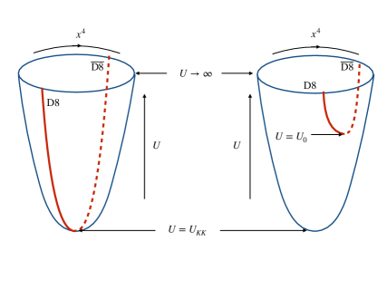
Figure 2: The D8-brane configuration in the bubble D4-brane background. Left: D8- and $\overline{\mathrm{D8}}$-branes are located at the antipodal points of $x^{4}$. Right: D8- and $\overline{\mathrm{D8}}$-branes are located at the non-antipodal points of $x^{4}$.

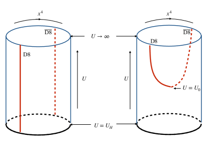
Figure 3: The D8-brane configuration in the black D4-brane background. Left: D8- and $\overline{\mathrm{D8}}$-branes are parallel located. Right: D8- and $\overline{\mathrm{D8}}$-branes are connected at $U=U_{0}$.

2.3 Gluon, quark and symmetries

As the dual theory in the D4/D8 model is expected to be QCD in the large $N_{c}$ limit, it is natural to identify the effective theory on $N_{c}$ D4-branes below $M_{KK}$ to the color sector in QCD which implies the gauge field $A_{\mu}^{\left(\mathrm{D4}\right)}$ on the D4-branes can be interpreted as gluon in holography. The reason is that the low-energy theory on $N_{c}$ D4-branes is $U\left(N_{c}\right)$ pure Yang-Mills theory and it has a SUGRA duality in the strong coupling region in the large $N_{c}$ limit as it is discussed in Section 2.1. We note that the Lorentz symmetry of the 10d spacetime breaks down to $SO\left(1+4\right)\times SO\left(5\right)$ when a stack of D4-branes is introduced. However the worldvolume symmetry of the D4-branes becomes $SO\left(1+3\right)$ since the D4-branes are compactified on a circle in the D4/D8 model. Furthermore, when the flavors as D8- and $\overline{\mathrm{D8}}$-branes are introduced, it is possible to create chiral fermions in the low-energy theory which can be obtained by analyzing the spectrum of $4-8$ or $4-\bar{8}$ string in R-sector (Ramond-sector). Both the spectra of $4-8$ and $4-\bar{8}$ string in R-sector contain spinors with positive and negative chirality as the representations of the Lorentz group $SO\left(1,3\right)$. Since the GSO (Gliozzi-Scherk-Olive) projection will remove the spinor with one of the chiralities in string theory, we can choose the spinor with positive and negative chirality as the massless fermionic modes (denoted by $q_{L,R}$) of $4-8$ and $4-\bar{8}$ string respectively which accordingly can be identified as the fundamental chiral quarks in the dual theory. We note that these chirally fermionic fields are complex spinors since the $4-8$ and $4-\bar{8}$ strings have two orientations. And they are also the fundamental representation of $U\left(N_{c}\right)$ and $U\left(N_{f}\right)$. The massless modes and symmetries in the D4/D8 system are collected in Table 2.

Fields	$U\left(N_{c}\right)$	$SO\left(1,3\right)$	$SO\left(5\right)$	$U\left(N_{f}\right)_{L}\times U\left(N_{f}\right)_{R}$
$A_{\mu}^{\left(\mathrm{D4}\right)}$	adj.	4	1	(1,1)
$q_{L}$	fund.	2+	1	(fund.,1)
$q_{R}$	fund.	2-	1	(1,fund.)
$a_{4}$	1	1	1	(1,1)
$\phi^{i}$	1	1	5	(1,1)

Table 2: The fields in the D4/D8 model. Here 2₊, 2_- denote the positive and negative chirality spinor representations of $SO\left(1,3\right)$. $a_{4}$ and $\phi^{i}$ are the trace parts of the gauge field along $x^{4}$ direction on the $N_{c}$ D4-branes and the transverse modes of the $N_{c}$ D4-branes which are decouple to the gluon and fundamental quarks in the low-energy theory.

Due to the above holographic correspondence, the chirally symmetric and broken phase in the dual theory can be identified respectively to the disconnected and connected configuration of the $\mathrm{D8/\overline{D8}}$-branes. It would be clear if we employ the configuration presented in Figure 2 for example. The effective action for the gauge fields $A_{\mu}^{\left(\mathrm{D4}\right)}$ and fundamental fermions $q_{L,R}$ on the $N_{c}$ D4-branes with $N_{f}$ $\mathrm{D8/\overline{D8}}$-branes can be evaluated by expanding the DBI action which leads to,

$$S= \int_{\mathrm{D4}}d^{5}x\sqrt{-g}\left[\delta\left(x^{4}-X_{L}\right)q_{L}^{\dagger}\bar{\sigma}^{\mu}\left(i\nabla_{\mu}+A_{\mu}\right)q_{L}+\delta\left(x^{4}-X_{R}\right)q_{R}^{\dagger}\bar{\sigma}^{\mu}\left(i\nabla_{\mu}+A_{\mu}\right)q_{R}\right]$$

$$-\frac{1}{4g_{\mathrm{YM}}^{2}}\int_{\mathrm{D4}}d^{5}x\sqrt{-g}\mathrm{Tr}F_{MN},\ M,N=0,1...4,$$ (2.31)

where $X_{L,R}$ denotes the intersection of the D4- and D8-branes, D4- and $\overline{\mathrm{D8}}$-branes and we have omitted the notation “D4” in $A_{\mu}$. As all the fields depend on $\left\{x^{\mu},x^{4}\right\}$, $q_{L}$ is identified to be $q_{R}$ if $X_{L}=X_{R}$ which leads to an action with single flavor symmetry $U\left(N_{f}\right)$. For the connected configurations, we can therefore see the D8- and $\overline{\mathrm{D8}}$-branes are separated at high energy ($U\rightarrow\infty$, $X_{L}\neq X_{R}$) according to the solutions (2.29) and (2.30), which leads to an approximated $U\left(N_{f}\right)_{L}\times U\left(N_{f}\right)_{R}$ chiral symmetry. However, at low energy $(U\rightarrow U_{0},X_{L}\rightarrow X_{R})$, D8- and $\overline{\mathrm{D8}}$-branes are joined into a single pair of D8-branes at $U=U_{0}$ ($X_{L}=X_{R}$) which implies the $U\left(N_{f}\right)_{L}\times U\left(N_{f}\right)_{R}$ symmetry breaks down to a single $U\left(N_{f}\right)$. This configuration of $\mathrm{D8/\overline{D8}}$-branes provides nicely a geometric interpretation of chiral symmetry in this model [56].

2.4 Mesons on the flavor brane

As meson is the bound state in the adjoint representation of the chiral symmetry group, it is identified as the gauge field on the flavor branes which is the massless mode excited by $8-8$ string. The reason is that the gauge field excited by $8-8$ (and $\bar{8}-\bar{8}$) is the generator of $U\left(N_{f}\right)_{L}$ (and $U\left(N_{f}\right)_{R}$). Hence we consider the gauge field on the flavor branes with non-zero components as $A_{M}=\left\{A_{\mu}\left(x,z\right),A_{z}\left(x,z\right)\right\},\mu=0,1...3$ in the bubble D4-brane background (2.16). We note that, while the supersymmetry on $N_{c}$ D4-branes breaks down by compactifying $x^{4}$ on a circle, there is not any mechanism to break down the supersymmetry on $\mathrm{D8/\overline{D8}}$-branes since $\mathrm{D8/\overline{D8}}$-branes are vertical to $x^{4}$. Therefore the $8-8$ string is supersymmetric leading to a super partner fermion $\Psi$ of the gauge field $A_{M}$ in the low-energy theory. And we will see in Appendix C, this supersymmetric fermion is Majorana spinor which leads to the fermionic meson (mesino) while they are absent in the realistic QCD.

Nonetheless let us assume the supersymmetry on the flavor branes somehow breaks down and the supersymmetric meson can be turned off in order to continue the discussion about the QCD sector of this model. Since the D8-branes are probes, the worldvolume gauge field is fluctuation. Thus the effective action for $A_{M}$ can be obtained by expanding (2.22) which, for Abelian case $N_{f}=1$, is

$$S_{\mathrm{D8}}= -T_{\mathrm{D8}}\int_{\mathrm{D8}}d^{9}xe^{-\phi}\sqrt{-\det\left[g_{ab}+\left(2\pi\alpha^{\prime}\right)F_{ab}\right]}$$

$$= -T_{\mathrm{D8}}\int_{\mathrm{D8}}d^{9}x\sqrt{-g}e^{-\phi}\left[1+\frac{1}{4}\left(2\pi\alpha^{\prime}\right)^{2}F_{MN}F^{MN}+\mathcal{O}\left(F^{4}\right)\right],$$ (2.32)

leading to the Yang-Mills (YM) action as,

$$S_{\mathrm{YM}}= -T_{\mathrm{D8}}\int_{\mathrm{D8}}d^{9}x\sqrt{-g}e^{-\phi}\frac{1}{4}\left(2\pi\alpha^{\prime}\right)^{2}F_{MN}F^{MN}$$

$$= -\frac{2}{3}R^{3/2}U_{KK}^{1/2}\left(2\pi\alpha^{\prime}\right)^{2}T_{\mathrm{D8}}\Omega_{4}\int d^{4}xdz\left(\frac{R^{3}}{4U}\eta^{\mu\rho}\eta^{\nu\sigma}F_{\mu\nu}F_{\rho\sigma}+\frac{9U^{3}}{8U_{KK}}\eta^{\mu\nu}F_{\mu z}F_{\nu z}\right)$$

$$= -\kappa\int d^{4}xdZ\left(\frac{1}{2}K^{-1/3}\eta^{\mu\rho}\eta^{\nu\sigma}F_{\mu\nu}F_{\rho\sigma}+KM_{KK}^{2}\eta^{\mu\nu}F_{\mu Z}F_{\nu Z}\right),$$ (2.33)

where we have used the Cartesian coordinates $z$ and dimensionless $Z$ defined as,

$$U^{3}=U_{KK}^{3}+U_{KK}z^{2},Z=\frac{z}{U_{KK}},K\left(Z\right)=1+Z^{2}=\frac{U^{3}}{U_{KK}^{3}},$$ (2.34)

and

$$\kappa=\frac{1}{3}R^{9/2}U_{KK}^{1/2}\left(2\pi\alpha^{\prime}\right)^{2}T_{\mathrm{D8}}\Omega_{4}=\frac{\lambda N_{c}}{216\pi^{3}},\lambda=g_{\mathrm{YM}}^{2}N_{c},$$ (2.35)

with the induced metric on the D8-branes as,

$$ds_{\mathrm{D8}}^{2}=\left(\frac{U}{R}\right)^{3/2}\eta_{\mu\nu}dx^{\mu}dx^{\nu}+\frac{4R^{3/2}U_{KK}}{9U^{5/2}}dz^{2}+R^{3/2}U^{1/2}d\Omega_{4}^{2}.$$ (2.36)

We have employed the configuration that $\mathrm{D8/\overline{D8}}$-branes are located at the antipodal points of $S^{1}$. Then, in order to obtain a 4d mesonic action, let us assume that $A_{\mu}\left(x,z\right),A_{z}\left(x,z\right)$ can be expanded in terms of complete sets $\left\{\psi_{n}\left(z\right),\phi_{n}\left(z\right)\right\}$ as,

$$A_{\mu}\left(x,z\right)=\sum_{n}B_{\mu}^{\left(n\right)}\left(x\right)\psi_{n}\left(z\right),A_{z}\left(x,z\right)=\sum_{n}\varphi^{\left(n\right)}\left(x\right)\phi_{n}\left(z\right),$$ (2.37)

where $B_{\mu}^{\left(n\right)}\left(x\right),\varphi^{\left(n\right)}\left(x\right)$ refers to the 4d meson field. To obtain a finite action, the normalization condition for $\psi_{n}\left(z\right)$ is chosen as,

$$2\kappa\int dZK^{-1/3}\psi_{n}\psi_{m}=\delta_{mn},$$ (2.38)

with the eigen equation ($n\geq 1$),

$$-K^{1/3}\partial_{Z}\left(K\partial_{Z}\psi_{n}\right)=\lambda_{n}\psi_{n},$$ (2.39)

where $\lambda_{n}$ is the associated eigen value. In this sense, the basic function $\phi_{n}\left(z\right)$ can be chosen as ($n\geq 1$),

$$\phi_{0}=\frac{1}{\sqrt{2\pi\kappa}}\frac{1}{U_{KK}M_{KK}}\frac{1}{K},\phi_{n}=m_{n}^{-1}\partial_{Z}\psi_{n},m_{n}=\lambda_{n}M_{KK}.$$ (2.40)

Keeping these in hand, impose (2.38) - (2.40) into (2.33) then define the vector field $V_{\mu}^{\left(n\right)}\left(x\right)$ by a gauge transformation,

$$V_{\mu}^{\left(n\right)}=B_{\mu}^{\left(n\right)}-m_{n}^{-1}\partial_{\mu}\varphi^{\left(n\right)},$$ (2.41)

the Yang-Mills action (2.33) reduces to a 4d effective action for mesons as,

$$S_{\mathrm{YM}}=-\kappa\int d^{4}x\left(\frac{1}{2}\partial_{\mu}\varphi^{\left(0\right)}\partial^{\mu}\varphi^{\left(0\right)}+\sum_{n=1}^{\infty}\left[\frac{1}{4}F_{\mu\nu}^{\left(n\right)}F^{\left(n\right)\mu\nu}+\frac{1}{2}m_{n}^{2}V_{\mu}^{\left(n\right)}V^{\left(n\right)\mu}\right]\right),$$ (2.42)

where $F_{\mu\nu}^{\left(n\right)}=\partial_{\mu}V_{\nu}^{\left(n\right)}-\partial_{\nu}V_{\mu}^{\left(n\right)}$. Accordingly, $\varphi^{\left(0\right)}$ can be interpreted as pion meson which is the Nambu-Goldstone boson associated to the chiral symmetry breaking. By analyzing the parity, it turns out that $\varphi^{\left(0\right)}$ is pseudo-scalar field as it is expected.

The above discussion implicitly assumes that the gauge field $A_{M}$ and its field strength $F_{MN}$ should vanish at $\left|z\right|\rightarrow\infty$ in order to obtain a finite 4d mesonic action. However there is an alternative gauge choice $A_{z}=0$ which is recognized as a gauge transformation

$$A_{M}\rightarrow A_{M}-\partial_{M}\Lambda,$$ (2.43)

to (2.37). Here $\Lambda$ is solved as,

$$\Lambda\left(x,z\right)=\varphi^{\left(0\right)}\left(x\right)\psi_{0}\left(z\right)+\sum_{n=1}^{\infty}m_{n}^{-1}\varphi^{\left(n\right)}\left(x\right)\psi_{n}\left(z\right),$$ (2.44)

where

$$\psi_{0}\left(z\right)=\int dz\phi_{0}\left(z\right)=\frac{1}{\sqrt{2\pi\kappa}}\frac{1}{M_{KK}}\arctan\left(\frac{z}{U_{KK}}\right).$$ (2.45)

Thus the components of $A_{M}$ under gauge condition $A_{z}=0$ becomes,

$$A_{\mu}\left(x,z\right)= -\partial_{\mu}\varphi^{\left(0\right)}\left(x\right)\psi_{0}\left(z\right)+\sum_{n=1}^{\infty}\left[B_{\mu}^{\left(n\right)}\left(x\right)-m_{n}^{-1}\partial_{\mu}\varphi^{\left(n\right)}\right]\psi_{n}\left(z\right)$$

$$= -\partial_{\mu}\varphi^{\left(0\right)}\left(x\right)\psi_{0}\left(z\right)+\sum_{n=1}^{\infty}V_{\mu}^{\left(n\right)}\left(x\right)\psi_{n}\left(z\right),$$

$$A_{z}\left(x,z\right)= 0.$$ (2.46)

In the region $\left|z\right|\rightarrow\infty$, the gauge potential $A_{\mu}\left(x,z\right)\rightarrow\pm\sqrt{\frac{\pi}{8\kappa}}\frac{1}{M_{KK}}$ which implies the gauge field strength remains to be vanished and the effective 4d action remains to be finite.

The above setup for mesons can be generalized into multi-flavor case by taking into account the non-Abelian version of (2.33),

$$S_{\mathrm{YM}}^{\left(N_{f}\right)}=-\kappa N_{f}\int d^{4}xdZ\left[\frac{1}{2}K^{-1/3}\eta^{\mu\rho}\eta^{\nu\sigma}\mathrm{Tr}\left(F_{\mu\nu}F_{\rho\sigma}\right)+KM_{KK}^{2}\eta^{\mu\nu}\mathrm{Tr}\left(F_{\mu Z}F_{\nu Z}\right)\right],$$ (2.47)

where $F_{MN}=\partial_{M}A_{N}-\partial_{N}A_{M}+\left[A_{M},A_{N}\right]$, $M,N=0,1,2,3,z$ is the gauge field strength of $U\left(N_{f}\right)$. As it has been discussed, in order to obtain a finite 4d action, the gauge field strength must vanish in the limit $\left|z\right|\rightarrow\infty$. Under the gauge condition $A_{z}=0$, $A_{\mu}$ must take asymptotically a pure gauge configuration for $\left|z\right|\rightarrow\infty$ as,

$$A_{\mu}\left(x,z\right)|_{z\rightarrow\pm\infty}\rightarrow\xi_{\pm}\left(x\right)\partial_{\mu}\xi_{\pm}^{-1}\left(x\right).$$ (2.48)

Compare this with (2.46), the gauge potential can be expanded with boundary condition (2.48) as,

$$A_{\mu}\left(x,z\right)= \xi_{+}\left(x\right)\partial_{\mu}\xi_{+}^{-1}\left(x\right)\psi_{+}\left(z\right)+\xi_{-}\left(x\right)\partial_{\mu}\xi_{-}^{-1}\left(x\right)\psi_{-}\left(z\right)+\sum_{n=1}^{\infty}V_{\mu}^{\left(n\right)}\left(x\right)\psi_{n}\left(z\right)$$

$$\equiv \alpha_{\mu}\left(x\right)\hat{\psi}_{0}\left(z\right)+\beta_{\mu}\left(x\right)+\sum_{n=1}^{\infty}V_{\mu}^{\left(n\right)}\left(x\right)\psi_{n}\left(z\right),$$ (2.49)

with

$$\psi_{\pm}= \frac{1}{2}\pm\hat{\psi}_{0},\hat{\psi}_{0}=\frac{1}{\pi}\arctan\left(\frac{z}{U_{KK}}\right).$$

$$\alpha_{\mu}\left(x\right)= \xi_{+}\left(x\right)\partial_{\mu}\xi_{+}^{-1}\left(x\right)-\xi_{-}\left(x\right)\partial_{\mu}\xi_{-}^{-1}\left(x\right)$$

$$\beta_{\mu}\left(x\right)= \frac{1}{2}\left[\xi_{+}\left(x\right)\partial_{\mu}\xi_{+}^{-1}\left(x\right)+\xi_{-}\left(x\right)\partial_{\mu}\xi_{-}^{-1}\left(x\right)\right].$$ (2.50)

To obtain the chiral Lagrangian for mesons from the Yang-Mills action (2.47), we identify the lowest vector meson field $V_{\mu}^{\left(n\right)}$ as the $\rho$ meson $V_{\mu}^{\left(1\right)}=\rho_{\mu}$ and choose the following gauge conditions

$$\xi_{+}^{-1}\left(x\right)=U\left(x\right),\xi_{-}\left(x\right)=1,$$ (2.51)

or

$$\xi_{+}^{-1}\left(x\right)=\xi_{-}\left(x\right)=\exp\left[i\pi\left(x\right)/f_{\pi}\right].$$ (2.52)

Inserting (2.49) into action (2.47) with the gauge condition (2.51), the 4d Yang-Mills action (2.47) includes a part of Skyrme model [61] as,

$$S_{\mathrm{YM}}^{\left(N_{f}\right)}=\int d^{4}x\left[\frac{f_{\pi}^{2}}{4}\mathrm{Tr}\left(U^{-1}\partial_{\mu}U\right)^{2}+\frac{1}{32e^{2}}\mathrm{Tr}\left(U^{-1}\partial_{\mu}U,U^{-1}\partial_{\mu}U\right)^{2}+...\right],$$ (2.53)

where the coupling constants $f_{\pi},e$ are given as,

$$f_{\pi}^{2} =6R^{3/2}U_{KK}^{1/2}T_{\mathrm{D8}}\Omega_{4}\left(2\pi\alpha^{\prime}\right)^{2}\int dz\frac{U\left(z\right)^{3}}{U_{KK}}\left(\partial_{z}\psi_{+}\right)^{2}=\frac{\lambda M_{KK}N_{c}}{54\pi^{2}},$$

$$e^{2} =\left[\frac{32}{3}R^{3/2}U_{KK}^{1/2}T_{\mathrm{D8}}\Omega_{4}\left(2\pi\alpha^{\prime}\right)^{2}\int dz\frac{R^{3}}{U\left(z\right)}\psi_{+}^{2}\left(\psi_{+}-1\right)^{2}\right]^{-1}=\frac{27\pi^{7}}{2b\lambda N_{c}},$$

$$b =\int\frac{dZ}{\left(1+Z^{2}\right)^{1/3}}\left(\arctan Z+\frac{\pi}{2}\right)^{2}\left(\arctan Z-\frac{\pi}{2}\right)^{2}\simeq 15.25.$$ (2.54)

And the interaction terms of $\pi,\rho$ mesons would be determined by the Yang-Mills action (2.47) with the gauge condition (2.52) as,

$$S_{\mathrm{YM}}^{\left(N_{f}\right)}= \int d^{4}x\mathrm{Tr}\left[-\partial_{\mu}\pi\partial^{\mu}\pi+\frac{1}{2}W_{\mu\nu}^{2}+m_{v}^{2}\rho_{\mu}^{2}+a_{\rho^{3}}\left[\rho_{\mu},\rho_{\nu}\right]W^{\mu\nu}+a_{\rho\pi^{2}}\left[\partial_{\mu}\pi,\partial_{\nu}\pi\right]W^{\mu\nu}\right]$$

$$+\mathcal{O}\left(\pi^{4},\rho_{\mu}^{4}\right),$$ (2.55)

where $W_{\mu\nu}$ is the gauge field strength of $\rho_{\mu}$ and the associated coupling constants are given by,

$$m_{\rho}^{2} =\Lambda_{1}M_{KK}^{2},a_{\rho^{3}}=\frac{\left(6\pi\right)^{3/2}}{\sqrt{\lambda N_{c}}}b_{\rho^{3}},a_{\rho\pi^{2}}=\frac{\pi\left(3\pi\right)^{3/2}}{M_{KK}^{2}\sqrt{2\lambda N_{c}}}b_{\rho\pi^{2}},$$

$$b_{\rho^{3}} \simeq 0.45,b_{\rho\pi^{2}}\simeq 1.6,\Lambda_{1}\simeq 0.67.$$ (2.56)

Therefore, we can reach to the meson tower or chiral Lagrangian starting with the D8-brane action which provides description of meson in holography.

To close this section, let us finally take a look at the WZ term presented in action (2.22), which can be integrated as,

$$S_{\mathrm{WZ}}^{\mathrm{D8}} =\frac{g_{s}}{3!}\left(2\pi\alpha^{\prime}\right)^{3}T_{\mathrm{D8}}\int_{\mathrm{D8}}C_{3}\wedge\mathrm{Tr}\left(F\wedge F\wedge F\right)$$

$$=\frac{g_{s}}{3!}\left(2\pi\alpha^{\prime}\right)^{3}T_{\mathrm{D8}}\int_{\mathrm{D8}}F_{4}\wedge\omega_{5}$$

$$=\frac{N_{c}}{24\pi^{2}}\mathrm{Tr}\int_{M_{4}\times\mathbb{R}}\omega_{5}\left(A\right).$$ (2.57)

Here $F_{4}=dC_{3}$ is the Ramond-Ramond field given in (2.14) and $\omega_{5}\left(A\right)$ is the Chern-Simons (CS) 5-form given as,

$$\omega_{5}\left(A\right)=AF^{2}-\frac{1}{2}A^{3}F+\frac{1}{10}A^{5},$$ (2.58)

where $F=dA+\frac{1}{2}\left[A,A\right]$ is the gauge field strength. Under the gauge transformation on the D8-brane,

$$\delta_{\Lambda}A=d\Lambda+\left[A,\Lambda\right],\delta_{\Lambda}F=\left[F,\Lambda\right],$$ (2.59)

we can compute

$$\mathrm{Tr}\left(\delta_{\Lambda}\omega_{5}\right) =\mathrm{Tr}\left[d\Lambda d\left(AdA+\frac{1}{2}A^{3}\right)\right]$$

$$=d\left(\mathrm{Tr}\left[\Lambda d\left(AdA+\frac{1}{2}A^{3}\right)\right]\right)$$

$$\equiv d\chi_{4}\left(\Lambda,A\right).$$ (2.60)

Hence by defining the boundary value of the gauge potential as,

$$A_{\mu}^{L}\left(x\right)=\lim_{z\rightarrow+\infty}A_{\mu}\left(x,z\right),A_{\mu}^{R}\left(x\right)=\lim_{z\rightarrow-\infty}A_{\mu}^{R}\left(x,z\right),$$ (2.61)

the WZ term reduces to the chiral anomaly of $U\left(N_{f}\right)_{L}\times U\left(N_{f}\right)_{R}$ in QCD as,

$$\delta_{\Lambda}S_{\mathrm{WZ}}^{\mathrm{D8}} =\frac{N_{c}}{24\pi^{2}}\mathrm{Tr}\int_{M_{4}\times\mathbb{R}}\delta_{\Lambda}\omega_{5}\left(A\right)=\frac{N_{c}}{24\pi^{2}}\int_{M_{4}}\chi_{4}\left(\Lambda,A\right)\big{|}_{z\rightarrow-\infty}^{z\rightarrow+\infty}$$

$$=\frac{N_{c}}{24\pi^{2}}\int_{M_{4}}\left[\chi_{4}\left(\Lambda_{L},A_{L}\right)-\chi_{4}\left(\Lambda_{R},A_{R}\right)\right].$$ (2.62)

And the formula for the chiral anomaly can also be expressed in the gauge condition $A_{z}=0$ which is to perform the gauge transformation

$$A^{g}=gAg^{-1}+gdg^{-1}.$$ (2.63)

Then the CS 5-form reduces to

$$\omega_{5}\left(A^{g}\right)=\omega_{5}\left(A\right)+\frac{1}{10}\left(gdg^{-1}\right)^{5}+d\alpha_{4},$$ (2.64)

where

$$\alpha_{4} =-\frac{1}{2}W_{1}\left(AdA+dAA+A^{3}\right)+\frac{1}{4}W_{1}AW_{1}A-W_{1}^{3}A,$$

$$W_{1} =dg^{-1}g.$$ (2.65)

Recall the formulas (2.49) in the gauge $A_{z}=0$ and choose the gauge condition (2.51), the WZ term (2.57) can be rewritten, after somewhat lengthy but straightforward calculations, as

$$S_{\mathrm{WZ}}^{\mathrm{D8}}=-\frac{N_{c}}{48\pi^{2}}\mathrm{Tr}\int_{M_{4}}L_{\mathrm{WZW}}-\frac{N_{c}}{240\pi^{2}}\mathrm{Tr}\int_{M_{4}\times\mathbb{R}}\left(gdg^{-1}\right)^{5},$$ (2.66)

where $L_{\mathrm{WZW}}$ is the Wess-Zumino-Witten (WZW) term in [62, 63] given as,

$$L_{\mathrm{WZW}}= \left[\left(A_{R}dA_{R}+dA_{R}A_{R}+A_{R}^{3}\right)\left(U^{-1}A_{L}U+U^{-1}dU\right)-\mathrm{p.c.}\right]$$

$$+\left(dA_{R}dU^{-1}A_{L}U-\mathrm{p.c.}\right)+\left[A_{R}\left(dU^{-1}U\right)^{3}-\mathrm{p.c.}\right]$$

$$+\frac{1}{2}\left[\left(A_{R}dU^{-1}U\right)^{2}-\mathrm{p.c.}\right]+\left[UA_{R}U^{-1}A_{L}dUdU^{-1}-\mathrm{p.c.}\right]$$

$$-\left[A_{R}dU^{-1}UA_{R}U^{-1}A_{L}U-\mathrm{p.c.}\right]+\frac{1}{2}\left(A_{R}U^{-1}A_{L}U\right)^{2}.$$ (2.67)

Note that “$\mathrm{p.c.}$” refers to the terms by exchanging $A_{L}\leftrightarrow A_{R},U\leftrightarrow U^{-1}$. And one can further work out the couplings to the vector mesons by using (2.49) with $A_{z}=0$.

2.5 The wrapped D4-brane and baryon vertex

In the $SU\left(N_{c}\right)$ gauge theory, a baryon vertex connects to $N_{c}$ external fundamental quarks with the color wave function combined together by an $N_{c}$-th antisymmetric tensor of $SU\left(N_{c}\right)$ group. Accordingly the baryon vertex in gauge-gravity duality is recognized as a D-brane wrapped on the internal sphere [26, 64]. To clarify this briefly, let us first recall the baryon vertex in the holographic duality between $\mathcal{N}=4$ super Yang-Mills theory and IIB string theory on $\mathrm{AdS}_{5}\times S^{5}$. As the fundamental quarks in the super Yang-Mills theory is created by the $N_{c}$ elementary superstrings in $\mathrm{AdS}_{5}\times S^{5}$, it is represented by the endpoints of elementary superstrings at the boundary of $\mathrm{AdS}_{5}$. Hence we need $N_{c}$ elementary superstrings with same orientation somehow to terminate in the $\mathrm{AdS}_{5}\times S^{5}$. On the other hand, since the baryon current must be conserved, one needs to find a source to cancel the $N_{c}$ charges (baryon charge) contributed by the $N_{c}$ elementary superstrings. To figure out these problems and work out a baryon vertex, a probe D5-brane wrapped on $S^{5}$ provides us a good answer. The $N_{c}$ elementary superstrings end on the D5-brane contributes $N_{c}$ to the D5-brane, however the WZ action for such a wrapped D5-brane,

$$S_{\mathrm{WZ}}^{\left(\mathrm{D5}\right)}\sim\int_{S^{5}\times\mathbb{R}}C_{4}F\sim\int_{S^{5}\times\mathbb{R}}F_{5}A\sim N_{c}\int_{\mathbb{R}}A,$$ (2.68)

(where $F_{5}=dC_{4}$ is the Ramond-Ramond field strength) nicely provides $N_{c}$ charges to cancel the charges given by $N_{c}$ elementary superstrings. Therefore the $A$ current would be conserved, which implies the D5-brane is a baryon vertex.

The construction of the baryon vertex can also been employed in the D4/D8 model which is identified as a D4-brane wrapped on $S^{4}$ with $N_{c}$ elementary superstrings ending on it. A remarkable point here is that the $\mathrm{D4}^{\prime}$-branes can be described equivalently by the instanton configuration of the gauge field on the D8-branes [65, 66]. To see this clearly, let us consider a $\mathrm{D}_{p}$-brane with its worldvolume gauge field strength $F$. According to (2.20), The WZ action for such a $\mathrm{D}_{p}$-brane includes a term as a source,

$$S_{\mathrm{WZ}}\sim g_{s}T_{D_{p}}\left(2\pi\alpha^{\prime}\right)^{2}\int C_{p-3}\mathrm{Tr}F^{2}.$$ (2.69)

For the single instanton configuration, the gauge field strength can be integrated as,

$$\mathrm{Tr}\int F^{2}=8\pi^{2}.$$ (2.70)

Hence (2.69) can be written as,

$$g_{s}T_{D_{p}}\left(2\pi\alpha^{\prime}\right)^{2}\int C_{p-3}\mathrm{Tr}F^{2}=g_{s}T_{D_{p-4}}\int C_{p-3},$$

giving rise to a same source included by a $\mathrm{D}_{p-4}$-brane. Accordingly, we obtain a simple and interesting conclusion here, that is the instanton in the $\mathrm{D}_{p}$-brane is the same object as a $\mathrm{D}_{p-4}$-brane inside it.

Let us return to the D4/D8 model, so it implies the $\mathrm{D4}^{\prime}$-branes as the baryon vertex are equivalent to the instanton in the $\mathrm{D8/\overline{D8}}$-branes. For multiple instantons, (2.70) is replaced by,

$$\mathrm{Tr}\int F^{2}=8\pi^{2}n,$$ (2.71)

where $n$ refers to the instanton number. Inserting the instanton configuration of the gauge field denoted as $A_{\mathrm{cl}}$ with a $U\left(N_{f}\right)_{V}$ fluctuation $\tilde{A}$ into the WZ action (2.57) of D8-brane, it reduces to

$$\frac{N_{c}}{8\pi^{2}}\int\tilde{A}\mathrm{Tr}F^{2}=nN_{c}\int\tilde{A},$$ (2.72)

which implies the instantons take $U\left(1\right)_{V}$ charge $nN_{c}$. Since the baryon number is defined as $1/N_{c}$ times the charge of the diagonal $U\left(1\right)_{V}$ subgroup of the $U\left(N_{f}\right)_{V}$ symmetry, it is obvious that the instanton number is equivalent to the baryon number in this holographic system.

Moreover, when (2.71) is integrated out to be a Chern-Simons 3-form $\omega_{3}$ as,

$$\int_{M_{4}}\mathrm{Tr}F^{2}=\int_{\partial M_{4}}\mathrm{Tr}\omega_{3}=\int\mathrm{Tr}\left(AF-\frac{1}{3}A^{3}\right),$$ (2.73)

the baryon number can be obtained as,

$$n=\frac{1}{8\pi^{2}}\mathrm{Tr}\int_{\mathbb{R}^{4}}F^{2}=\mathrm{Tr}\int_{\mathbb{R}^{3}}\omega_{3}|_{z\rightarrow-\infty}^{z\rightarrow+\infty}=-\frac{1}{24\pi^{2}}\mathrm{Tr}\int_{\mathbb{R}^{3}}\left(U^{-1}dU\right)^{3},$$ (2.74)

where we have imposed the similar boundary condition as it is given in (2.51),

$$\lim_{z\rightarrow+\infty}A_{\mu}\left(x^{\mu},z\right)=U^{-1}\left(x^{i}\right)\partial_{i}U\left(x^{i}\right),\lim_{z\rightarrow-\infty}A_{\mu}\left(x^{\mu},z\right)=0.$$ (2.75)

The (2.74) gives the winding number of $U$ which means the homotopy is $\pi_{3}\left[U\left(N_{f}\right)\right]\simeq\mathbb{Z}$. And it agrees with the baryon number charge in the Skyrme model [62, 67].

The baryon mass $m_{B}$ can be roughly obtained by evaluating the energy carried by the $\mathrm{D4}^{\prime}$-branes which can be read from its DBI action as,

$$S_{\mathrm{D4}^{\prime}}= -T_{\mathrm{D4}}\int dx^{0}d\Omega_{4}e^{-\phi}\sqrt{-g_{00}g_{S^{4}}}$$

$$= -\frac{1}{27}M_{KK}\lambda N_{c}^{2}\int_{\mathbb{R}}dx^{0},$$

$$= -m_{B}\int_{\mathbb{R}}dx^{0}$$ (2.76)

where the bubble D4-brane background has been chosen for the confined property of baryon and $g_{S^{4}}$ refers to the metric on $S^{4}$ presented in (2.16). This formula illustrates a stable position of the baryonic $\mathrm{D4}^{\prime}$-brane by minimizing its energy, which is $U=U_{KK}$ since the bubble geometry shrinks at $U=U_{KK}$. In the black D4-brane, one can follow the same formula (2.76) to evaluate the baryon mass. However, if the baryonic $\mathrm{D4}^{\prime}$-brane is the only probe brane, it can not stay at $U=U_{H}$ stably in the black D4-brane background since gravity will pull it into the horizon. In this sense, the baryon vertex exists in the bubble D4-brane background only and it is consistent with its property of confinement. When the probe $\mathrm{D8/\overline{D8}}$-branes are embedded into the bulk geometry, due to the balance condition, the baryonic $\mathrm{D4}^{\prime}$-brane can be restricted inside the D8-branes if $\mathrm{D8/\overline{D8}}$-branes are connected, as it is displayed in Figure 4.

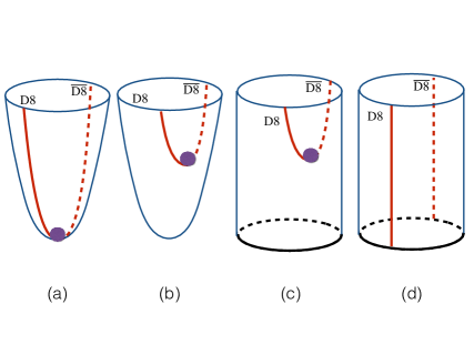
Figure 4: Various D-brane configurations in the D4/D8 model. Purple refers to the baryon vertex ($\mathrm{D4}^{\prime}$-brane) locates at the stable position. When the $\mathrm{D8/\overline{D8}}$-branes are connected as (a), (b), (c), the baryon vertex can locate stably at the connected position inside the $\mathrm{D8/\overline{D8}}$-branes. There is not a stable position for baryon vertex if $\mathrm{D8/\overline{D8}}$-branes are parallel as (d).

Therefore it can be described equivalently by the instanton configuration on the D8-branes.

To obtain the baryon mass or baryon spectrum in this model, it is worth searching for an exact instanton solution for the gauge field on the D8-branes. As baryon lives in the low-energy region of QCD, we may find an approximated solution for the instanton configuration in the strong coupling limit i.e. $\lambda\rightarrow\infty$. To this goal, let us take a look at the gauge field on the D8-branes whose dynamic is described by the Yang-Mills action (2.33) plus the Chern-Simons action presented in (2.57) . Since the size of instanton is of order $\lambda^{-1/2}$, it would be convenient to rescale the coordinate $\left\{x^{0},x^{i},z\right\}$ and the gauge potential $A$ as,

$$x^{M}\rightarrow\lambda^{-1/2}x^{M},\ x^{0}\rightarrow x^{0}$$

$$A_{M}\rightarrow\lambda^{1/2}A_{M},\ A_{0}\rightarrow A_{0}$$

$$F_{MN}\rightarrow\lambda F_{MN},\ F_{0M}\rightarrow\lambda^{1/2}F_{0M},$$ (2.77)

where $M,N=1,2,3,z$. In the large $\lambda$ limit, the Yang-Mills action (2.33) can be expanded as,

$$S_{\mathrm{YM}}= -\frac{\kappa}{\lambda}\int d^{4}xdz\mathrm{Tr}\left[\frac{\lambda}{2}F_{MN}^{2}+\left(-\frac{z^{2}}{6}F_{ij}^{2}+z^{2}F_{iz}^{2}-F_{0M}^{2}\right)+\mathcal{O}\left(\lambda^{-1}\right)\right]$$

$$-\frac{\kappa}{2\lambda}\int d^{4}xdz\left[\frac{\lambda}{2}\hat{F}_{MN}^{2}+\left(-\frac{z^{2}}{6}\hat{F}_{ij}^{2}+z^{2}\hat{F}_{iz}^{2}-\hat{F}_{0M}^{2}\right)+\mathcal{O}\left(\lambda^{-1}\right)\right],$$ (2.78)

while the Chern-Simons action (2.57) remains under the rescaling (2.77). We have employed the D-brane configuration presented in (a) of Figure 4. The $U\left(N_{f}\right)$ group is decomposed as $U\left(N_{f}\right)\simeq U\left(1\right)\times SU\left(N_{f}\right)$ and correspondingly its generator is decomposed as,

$$A+\frac{1}{\sqrt{2N_{f}}}\hat{A}=A^{a}t^{a}+\frac{1}{\sqrt{2N_{f}}}\hat{A},$$ (2.79)

where $\hat{A},A$ refers to the generators of $U\left(1\right)$, $SU\left(N_{f}\right)$ respectively and $t^{a}$ ($a=1,2...N_{f}^{2}-1$) are the normalized bases satisfying

$$\mathrm{Tr}\left(t^{a}t^{b}\right)=\frac{1}{2}\delta^{ab}.$$ (2.80)

So the Chern-Simons action (2.57) can be derived as,

$$S_{\mathrm{CS}}= \frac{N_{c}}{24\pi^{2}}\int\omega_{5}^{SU\left(N_{f}\right)}\left(A\right)+\frac{N_{c}}{24\pi^{2}}\sqrt{\frac{2}{N_{f}}}\epsilon_{MNPQ}\int d^{4}xdz\bigg{[}\frac{3}{8}\hat{A}_{0}\mathrm{Tr}\left(F_{MN}F_{PQ}\right)$$

$$-\frac{3}{2}\hat{A}_{M}\mathrm{Tr}\left(\partial_{0}A_{N}F_{PQ}\right)+\frac{3}{4}\hat{F}_{MN}\mathrm{Tr}\left(A_{0}F_{PQ}\right)+\frac{1}{16}\hat{A}_{0}\hat{F}_{MN}\hat{F}_{PQ}-\frac{1}{4}\hat{A}_{M}\hat{F}_{0N}\hat{F}_{PQ}$$

$$+\left(\mathrm{total\ derivatives}\right)\bigg{]}.$$ (2.81)

And the equation of motion for $\hat{A},A$ can be derived by varying action (2.78) plus (2.81) which allows an instanton solution as,

$$A_{M}^{\mathrm{cl}}=-if\left(\xi\right)g\left(x\right)\partial_{M}g^{-1},$$ (2.82)

where

$$f\left(\xi\right) =\frac{\xi^{2}}{\xi^{2}+\rho^{2}},\xi=\sqrt{\left(x^{M}-X^{M}\right)^{2}},$$

$$g\left(x\right) =\left(\begin{array}[]{cc}g^{SU\left(2\right)}\left(x\right)&0\\ 0&\mathbf{1}_{N_{f}-2}\end{array}\right),g^{SU\left(2\right)}\left(x\right)=\frac{1}{\xi}\left[\left(z-Z\right)\mathbf{1}_{2}-i\left(x^{i}-X^{i}\right)\tau^{i}\right].$$ (2.85)

Here $\mathbf{1}_{N}$ is an $N\times N$ identity matrix and $\tau^{i}$’s are the Pauli matrices. The position and the size of the instanton are denoted by the constants $X^{M}=\left\{X^{i},Z\right\}$ and $\rho$ respectively to which have been rescaled as (2.77). The configuration (2.82) (2.85) is the Belavin–Polyakov–Schwarz–Tyupkin (BPST) solution embedding into $SU\left(N_{f}\right)$ which represents the $SU\left(2\right)$ Euclidean instanton, and one may verify this solution satisfies (2.70). Then the $U\left(1\right)$ part of the gauge field is solved as,

$$\hat{A}_{0}^{\mathrm{cl}}=\sqrt{\frac{2}{N_{f}}}\frac{1}{8\pi^{2}a}\frac{1}{\xi^{2}}\left[1-\frac{\rho^{4}}{\left(\xi^{2}+\rho^{2}\right)^{2}}\right],\ \hat{A}_{M}^{\mathrm{cl}}=0.$$ (2.86)

which leads to a non-zero $A_{0}$ as,

$$A_{0}^{\mathrm{cl}}=\frac{1}{16\pi^{2}a}\frac{1}{\xi^{2}}\left[1-\frac{\rho^{4}}{\left(\xi^{2}+\rho^{2}\right)^{2}}\right]\left(\mathcal{P}_{2}-\frac{2}{N_{f}}\mathbf{1}_{N_{f}}\right),$$ (2.87)

where $\mathcal{P}_{2}$ is an $N_{f}\times N_{f}$ matrix $\mathcal{P}_{2}=\mathrm{diag}\left(1,1,0,...0\right)$.

Keeping these in hand, it is possible to evaluate the classical baryon mass through the soliton mass $M$ with respect to the D8-brane action as $S\left[A^{\mathrm{cl}}\right]=-\int Mdt$ which is obtained as,

$$M=8\pi^{2}\kappa+\frac{8\pi^{2}\kappa}{\lambda}\left(\frac{\rho^{2}}{6}+\frac{Z^{2}}{3}+\frac{1}{320\pi^{4}a^{2}\rho^{2}}\right),$$ (2.88)

by inserting (2.82) - (2.87) into action (2.78) plus (2.81). On the other hand, since the low-energy effective theory on the D8-branes can reduce to Skyrme model, we can further employ the idea in the Skyrme model of baryon, which is identified as the excitation of the collective modes, in order to search for the baryon spectrum. The classically effective Lagrangian for baryon describing the dynamics of the collective coordinates $\mathcal{X}^{\alpha}$ in the moduli space by the one instanton solution. which refers to the world line element with a baryonic potential $U\left(\mathcal{X}^{\alpha}\right)$ in the moduli space

$$L\left(\mathcal{X}^{\alpha}\right)=\frac{m_{X}}{2}\mathcal{G}_{\alpha\beta}\dot{\mathcal{X}}^{\alpha}\dot{\mathcal{X}}^{\beta}-U\left(\mathcal{X}^{\alpha}\right)+\mathcal{O}\left(\lambda^{-1}\right),$$ (2.89)

where “$\cdot$” refers to the derivative respected to time, the collective coordinates $\mathcal{X}^{\alpha}$ denotes to $\left\{X^{M},\rho,y^{a}\right\}$ and $W=y^{a}t^{a}$ is the $SU\left(N_{f}\right)$ orientation of the instanton. The potential $U\left(\mathcal{X}^{\alpha}\right)$ is the classical soliton mass given by $S\left[A^{\mathrm{cl}}\right]=-\int dtU\left(\mathcal{X}^{\alpha}\right)$. The basic idea to quantize the classical Lagrangian (2.89) is to move slowly the classical soliton so that the collective coordinates $\mathcal{X}^{\alpha}$ are promoted to be time-dependent [69]. Approximately, the $SU\left(N_{f}\right)$ gauge field potential is becomes time-dependent by a gauge transformation,

$$A_{M}\left(t,x\right) =W\left(t\right)A_{M}^{\mathrm{cl}}\left(x,\mathcal{X}^{\alpha}\right)W\left(t\right)^{-1}-iW\left(t\right)\partial_{M}W\left(t\right)^{-1},$$

$$A_{0}\left(t,x\right) =W\left(t\right)A_{0}^{\mathrm{cl}}\left(x,\mathcal{X}^{\alpha}\right)W\left(t\right)^{-1}+\Delta A_{0},$$

$$\hat{A}_{M}\left(t,x\right) =0,\ \hat{A}_{0}\left(t,x\right)=\hat{A}_{0}^{\mathrm{cl}}\left(t,x\right),$$ (2.90)

and the associated field strength becomes,

$$F_{MN}= W\left(t\right)F_{MN}^{\mathrm{cl}}W\left(t\right)^{-1},$$

$$F_{0M}= W\left(t\right)\left(\dot{\mathcal{X}}^{\alpha}\frac{\partial}{\partial\mathcal{X}^{\alpha}}A_{M}^{\mathrm{cl}}-D_{M}^{\mathrm{cl}}\Sigma-D_{M}^{\mathrm{cl}}A_{0}^{\mathrm{cl}}\right)W\left(t\right)^{-1},$$

$$\hat{F}_{0M}= \hat{F}_{0M}^{\mathrm{cl}},\ \hat{F}_{MN}=\hat{F}_{MN}^{\mathrm{cl}},$$ (2.91)

where

$$D_{M}^{\mathrm{cl}}A_{0} =\partial_{M}A_{0}+i\left[A_{M}^{\mathrm{cl}},A_{0}\right],$$

$$\Sigma =W\left(t\right)^{-1}\Delta A_{0}W\left(t\right)-i\dot{W}\left(t\right)^{-1}W\left(t\right).$$ (2.92)

$\Delta A_{0}$ must be determined by its equation of motion as,

$$D_{M}^{\mathrm{cl}}\left(\dot{X}^{N}\frac{\partial}{\partial X^{N}}A_{M}^{\mathrm{cl}}+\dot{\rho}\frac{\partial}{\partial\rho}A_{M}^{\mathrm{cl}}-D_{M}^{\mathrm{cl}}\Sigma\right)=0.$$ (2.93)

While for generic $N_{f}$, the exact solution for $\Sigma$ may be out of reach, the solution with $N_{f}=2,3$ is collected respectively in [27, 28]. Accordingly the Lagrangian of the collective modes is given by

$$S\left[\mathcal{A}\right]-S\left[\mathcal{A}^{\mathrm{cl}}\right] =\int dt\left[L_{\mathrm{YM}}\left(\mathcal{X}^{\alpha}\right)+L_{\mathrm{CS}}\left(\mathcal{X}^{\alpha}\right)\right]=\int dtL\left(\mathcal{X}^{\alpha}\right)$$

$$S_{\mathrm{YM}}\left[\mathcal{A}\right]-S_{\mathrm{YM}}\left[\mathcal{A}^{\mathrm{cl}}\right] =\int dtL_{\mathrm{YM}}\left(\mathcal{X}^{\alpha}\right),$$

$$S_{\mathrm{CS}}\left[\mathcal{A}\right]-S_{\mathrm{CS}}\left[\mathcal{A}^{\mathrm{cl}}\right] =\int dtL_{\mathrm{CS}}\left(\mathcal{X}^{\alpha}\right),$$ (2.94)

which leads to,

$$L\left(\mathcal{X}^{\alpha}\right) =-M+aN_{c}\mathrm{Tr}\int d^{3}xdz\left(\dot{X}^{N}F_{MN}^{\mathrm{cl}}+\dot{\rho}\frac{\partial}{\partial\rho}A_{M}-\dot{X}^{N}D_{M}^{\mathrm{cl}}A_{N}^{\mathrm{cl}}-D_{M}^{\mathrm{cl}}\Sigma\right)^{2}+\mathcal{O}\left(\lambda^{-1}\right)$$

$$=-M_{0}+\frac{m_{X}}{2}\delta_{ij}\dot{X}^{i}\dot{X}^{j}+L_{Z}+L_{\rho}+L_{\rho W}+\mathcal{O}\left(\lambda^{-1}\right),$$ (2.95)

where

$$L_{Z}= \frac{m_{Z}}{2}\left(\dot{Z}^{2}-\omega_{Z}^{2}Z^{2}\right),L_{\rho}=\frac{m_{\rho}}{2}\left(\dot{\rho}-\omega_{\rho}^{2}\rho^{2}\right)-\frac{K}{m_{\rho}\rho^{2}},$$

$$L_{\rho W}= \frac{m_{\rho}\rho^{2}}{2}\sum_{a}C_{a}\left[\mathrm{Tr}\left(-iW^{-1}\dot{W}t^{a}\right)\right]^{2},a=1,2...N_{f}^{2}-1$$ (2.96)

and

$$M_{0}=8\pi^{2}\kappa,m_{X}=m_{Z}=\frac{m_{\rho}}{2}=8\pi^{2}\kappa\lambda^{-1},K=\frac{2}{5}N_{c}^{2},\omega_{Z}^{2}=4\omega_{\rho}^{2}=\frac{2}{3}.$$ (2.97)

Here we note that the formulas are in the unit of $M_{KK}=1$, $C_{a}$’s are constants dependent on the $SU\left(N_{f}\right)$ instanton solution and the metric of the moduli space can be further obtained by comparing (2.95) with (2.89). For example, we have $C_{1,2,3}=1$ for $N_{f}=2$, and $C_{1,2,3}=1,C_{4,5,6,7}=1/2,C_{8}=0$ for $N_{f}=3$. Afterwards, the baryon states can be obtained by quantizing the Lagrangian (2.95) that is to replace the derivative term by $\dot{X}^{\alpha}\rightarrow-\frac{i}{m_{X}}\partial_{\alpha}$ straightforwardly. Hence the quantized Hamiltonian associated to (2.95) is collected as,

$$H= M_{0}+H_{Z}+H_{\rho}+H_{\rho W},$$

$$H_{Z}= -\frac{1}{2m_{Z}}\partial_{Z}^{2}+\frac{1}{2}m_{Z}\omega_{Z}^{2}Z^{2},$$

$$H_{\rho}= -\frac{1}{2m_{\rho}}\frac{1}{\rho^{\eta}}\partial_{\rho}\left(\rho^{\eta}\partial_{\rho}\right)+\frac{1}{2}m_{\rho}\omega_{\rho}^{2}\rho^{2}+\frac{K}{m_{\rho}\rho^{2}},$$

$$H_{\rho W}= \frac{m_{\rho}\rho^{2}}{2}\sum_{a}C_{a}\left[\mathrm{Tr}\left(-iW^{-1}\dot{W}t^{a}\right)\right]^{2}=\frac{2}{m_{\rho}\rho^{2}}\sum_{a}C_{a}\left(J^{a}\right)^{2},$$ (2.98)

where $\eta=N_{f}^{2}-1$ and $J^{a}$’s are the operators of the angular momentum of $SU\left(N_{f}\right)$. The baryon spectrum can be finally obtained by evaluating the eigen values of the Hamiltonian (2.98) which takes a fortunately analytical formula [27, 28].

2.6 Gravitational wave as glueball

According to AdS/CFT and gauge-gravity duality [29, 30, 31, 32], the glueball operator $\hat{O}$ can be identified as the source of gravitational fluctuation in bulk since it is included in energy-momentum tensor of Yang-Mills theory in the dual theory as $\hat{O}\sim F_{\mu\nu}F^{\mu\nu}\sim T_{\mu\nu}$ coupling to metric. Thus due to the confined property of glueball, we can choose the bubble D4-brane background (2.16) compactified on a circle with gravitational fluctuation in order to investigate glueball in holography.

The dual field to the glueball operator is the gravitational fluctuation coupling the energy-momentum which therefore refers to the gravitational polarization. By employing the relation of 11d M-theory and 10d type IIA string theory in Section 2.1, it would be convenient to find the gravitational polarization in 11d theory. For example, the lowest exotic scalar glueball with quantum number $J^{CP}=0^{++}$ corresponds to the exotic polarizations of the bulk gravitational polarization and its 11d components are given as ($\mu,\nu=0,1,2,3$),

$$\delta g_{44} = -\frac{r^{2}}{L^{2}}f\left(r\right)H_{E}\left(r\right)G_{E}\left(x\right),$$

$$\delta g_{\mu\nu} = \frac{r^{2}}{L^{2}}H_{E}\left(r\right)\left[\frac{1}{4}\eta_{\mu\nu}-\left(\frac{1}{4}+\frac{3r_{KK}^{6}}{5r^{6}-2r_{KK}^{6}}\right)\frac{\partial_{\mu}\partial_{\nu}}{M_{E}^{2}}\right]G_{E}\left(x\right),$$

$$\delta g_{55} = \frac{r^{2}}{4L^{2}}H_{E}\left(r\right)G_{E}\left(x\right),$$

$$\delta g_{rr} = -\frac{L^{2}}{r^{2}}\frac{1}{f\left(r\right)}\frac{3r_{KK}^{6}}{5r^{6}-2r_{KK}^{6}}H_{E}\left(r\right)G_{E}\left(x\right),$$

$$\delta g_{r\mu} = \frac{90r^{7}r_{KK}^{6}}{M_{E}^{2}L^{2}\left(5r^{6}-2r_{KK}^{6}\right)^{2}}H_{E}\left(r\right)\partial_{\mu}G_{E}\left(x\right),$$ (2.99)

where $H_{E}\left(r\right)$ must be determined by its eigen equation given by,

$$\frac{1}{r^{3}}\frac{d}{dr}\left[r\left(r^{6}-r_{KK}^{6}\right)\frac{d}{dr}H_{E}\left(r\right)\right]+\left[\frac{432r^{2}r_{KK}^{12}}{\left(5r^{6}-2r_{KK}^{6}\right)^{2}}+L^{4}M_{E}^{2}\right]H_{E}\left(r\right)=0,$$ (2.100)

and $G_{E}\left(x\right)$ refers to the 4d glueball field. By imposing metric with gravitational fluctuation (2.99) as $g_{MN}=g_{MN}^{\left(0\right)}+\delta g_{MN}$ and solution of $C_{3}$ into 11d SUGRA action (2.1), we can obtain

$$S_{\mathrm{SUGRA}}^{11\mathrm{d}}=-\frac{1}{2}\mathcal{C}_{E}\beta_{4}\beta_{5}\int d^{4}x\left[\left(\partial_{\mu}G_{E}\right)^{2}+M_{E}^{2}G_{E}^{2}\right],$$ (2.101)

representing the standard kinetic action for scalar glueball field $G_{E}$, where $\beta_{5}$, $g_{MN}^{\left(0\right)}$ refers respectively to the size of $x^{5}$ and the bubble version of (2.10). $\mathcal{C}_{E}$ is a numerical constant given by,

$$\mathcal{C}_{E} =0.057396\left[H_{E}\left(r_{KK}\right)\right]^{2}\frac{r_{KK}^{4}}{L^{3}},$$

$$\left[H_{E}\left(r_{KK}\right)\right]^{-1} =0.0069183\lambda^{1/2}N_{c}M_{KK}.$$ (2.102)

Hence the eigen value of (2.100) determines the mass spectrum of exotic scalar glueball. The mass spectrum for various glueballs can be obtained by taking into account different gravitational polarizations e.g. dilatonic scalar glueball with $J^{CP}=0^{++}$,

$$\delta G_{11,11} =-3\frac{r^{2}}{L^{2}}H_{D}\left(r\right)G_{D}\left(x\right),$$

$$\delta G_{\mu\nu} =\frac{r^{2}}{L^{2}}H_{D}\left(r\right)\left[\eta^{\mu\nu}-\frac{\partial^{\mu}\partial^{\nu}}{M_{D}^{2}}\right]G_{D}\left(x\right),$$ (2.103)

and tensor glueball with $J^{CP}=2^{++}$,

$$\delta G_{\mu\nu}=-\frac{r^{2}}{L^{2}}H_{T}\left(r\right)T_{\mu\nu}\left(x\right).$$ (2.104)

The eigen equations for $H_{D}\left(r\right)$ and $H_{T}\left(r\right)$ are given as,

$$\frac{1}{r^{3}}\frac{d}{dr}\left[r\left(r^{6}-r_{KK}^{6}\right)\frac{d}{dr}H_{D,T}\left(r\right)\right]+L^{4}M_{D,T}^{2}H_{D,T}\left(r\right)=0,$$ (2.105)

which determines the mass spectrum of dilatonic scalar and tensor glueball. The mass spectrum of various glueballs are collected in Table 3 for the reader’s convenience. The labels $\mathrm{S,T,V,N,M,L}$ refer to the solutions for six independent wave equations for various scalar, vector tensor modes of glueballs.

Mode	$\mathrm{S}_{4}$	$\mathrm{T}_{4}$	$\mathrm{V}_{4}$	$\mathrm{N}_{4}$	$\mathrm{M}_{4}$	$\mathrm{L}_{4}$
$J^{PC}$	$0^{++}$	$0^{++}/2^{++}$	$0^{-+}$	$1^{+-}$	$1^{--}$	$0^{++}$
$n=0$	7.30835	22.0966	31.9853	53.3758	83.0449	115.002
$n=1$	46.9855	55.5833	72.4793	109.446	143.581	189.632
$n=2$	94.4816	102.452	126.144	177.231	217.397	227.283
$n=3$	154.963	162.699	193.133	257.959	304.531	378.099
$n=4$	228.709	236.328	273.482	351.895	405.011	492.171

Table 3: Glueball mass spectrum $m_{n}^{2}$ of $\mathrm{AdS}_{7}$ in the units of $r_{KK}^{2}/L^{4}=M_{KK}^{2}/9$ in [32].

And this model predicts the properties of glueball in a very simple and powerful way.

3 Developments and holographic approaches to QCD

In this section, we will review some holographic approaches to QCD by using the D4/D8 model and some developments of this model in recent years which includes basically the topics about phase transition, heavy flavor, hadron interaction and theta angle in QCD.

3.1 QCD deconfinement transition

While the confinement phase of QCD corresponds to the bubble D4-brane geometry given in (2.16), it is less clear whether the black D4-brane background (2.14) corresponds to the deconfinement phase in holography exactly [58, 59]. This issue is recognized by investigating the associated Wilson loop in the bubble (2.16) and black brane background (2.14) respectively. Nonetheless, it would be interesting to compare the deconfinement transition in QCD with the Hawking-Page transition in D4-brane system through the gauge-gravity duality to find a holographic description of the deconfinement transition exactly. To this goal, let us first recall the holographic relation between the partition functions $Z$ of the bulk gravity and its dual field theory,

$$Z=e^{-F}=e^{-S_{\mathrm{SUGRA}}^{ren}},$$ (3.1)

which implies the classical (onshell) renormalized SUGRA action $S_{\mathrm{SUGRA}}^{ren}$ is equivalent to the free energy $F$ of the dual theory (in the Euclidean version). The classical SUGRA action $S_{\mathrm{SUGRA}}^{ren}$ can be collected by

$$S_{\mathrm{SUGRA}}^{ren}=S_{\mathrm{IIA}}^{E}+S_{\mathrm{GH}}+S_{\mathrm{CT}}^{\mathrm{bulk}},$$ (3.2)

where $S_{\mathrm{IIA}}^{E}$ refers to the Euclidean version of IIA SUGRA action given in (2.15). And $S_{\mathrm{GH}}$ refers to the standard Gibbons-Hawking term given by [71],

$$S_{\mathrm{GH}}=\frac{1}{\kappa_{10}^{2}}\int_{\partial\mathcal{M}}e^{-2\Phi}\sqrt{h}K,$$ (3.3)

where $h_{MN}$ refers to the metric on the holographic boundary $\partial\mathcal{M}$ with $\partial\mathcal{M}=\left\{r=\varepsilon\right\}$ for $\varepsilon\rightarrow 0$, and

$$K=h^{MN}\nabla_{M}n_{N}=-\frac{1}{\sqrt{\left|g\right|}}\partial_{r}\left(\frac{\sqrt{\left|g\right|}}{\sqrt{g_{rr}}}\right)\big{|}_{r=\varepsilon},$$ (3.4)

is trace of the extrinsic curvature. $S_{\mathrm{CT}}^{\mathrm{bulk}}$ refers to the counterterm of the bulk fields presented in action (2.15) given as [72],

$$S_{\mathrm{CT}}^{\mathrm{bulk}}=-\frac{5}{2\kappa_{10}^{2}}\frac{g_{s}^{1/3}}{R}\int d^{9}xe^{-7\Phi/3}\sqrt{h}.$$ (3.5)

Using (3.2) - (3.5) by picking up the bubble (2.16) and black brane background (2.14) solution respectively, we can obtain the free energy of the dual theory by a simple formula as,

$$F_{\mathrm{conf.}} =S_{\mathrm{SUGRA}}^{ren,\mathrm{bub}}=-\frac{2N_{c}^{2}M_{KK}^{4}\lambda V_{4}}{3^{7}\pi^{2}},$$

$$F_{\mathrm{deconf}.} =S_{\mathrm{SUGRA}}^{ren,\mathrm{black}}=-\frac{2^{7}N_{c}^{2}T^{6}\pi^{4}\lambda V_{4}}{3^{7}M_{KK}^{2}},$$ (3.6)

where $V_{4}$ refers to the volume of $\mathbb{R}^{4}$, $T$ is the Hawking temperature in the black D4-brane solution (2.16). Comparing the free energies given in (3.6), we obtain the critical temperature by $F_{\mathrm{conf.}}=F_{\mathrm{deconf}.}\left(T=T_{c}\right)$ for the Hawking-Page transition as,

$$T_{c}=\frac{M_{KK}}{2\pi},$$ (3.7)

which is expected to be the deconfinement transition in QCD in the large $N_{c}$ limit. While this may be a trivial result for QCD, it is theoretically expected in gravity side since the bubble solution (2.14) is obtained by a double Wick rotation to the black brane solution (2.16) i.e. (3.7) means exactly $\beta_{4}=\beta_{T}$. However, this does not mean that Hawking-Page transition has nothing to do with the QCD deconfinement transition because the fundamental flavored matter has not been taken into account.

In order to obtain a critical temperature close to the realistic QCD with the D4/D8 model, the flavored matter on the D8-branes must somehow contribute to the free energy. It means in the gravity side, flavor branes have to back react to the bulk geometry thus they would not be probes. For such a holographic setup, we have to require $N_{f}/N_{c}$ is fixed in the large $N_{c}$ limit in order to go beyond the probe approximation for the flavor branes. Besides we further need $N_{f}/N_{c}\ll 1$ otherwise the dynamics of the dual theory is determined by flavors instead of colors, and in the gravity side $N_{f}/N_{c}\ll 1$ is also necessary since $N_{c}$ D4-branes must dominate the bulk geometry otherwise the holographic duality given in the previous sections would not be valid. Then the next step is to confirm the embedding configuration of the $\mathrm{D8/\overline{D8}}$-branes. Since the configuration of the $\mathrm{D8/\overline{D8}}$-branes relates to the chiral symmetry discussed in Section 2.2 - 2.3, we can identify respectively the bubble D4-brane background where $\mathrm{D8/\overline{D8}}$-branes are located at the antipodal points of $x^{4}$ (the left one in Figure 2) as the confined phase with broken chiral symmetry and the black D4-brane background where $\mathrm{D8/\overline{D8}}$-branes are parallel (the left one in Figure 3) as the deconfined phase with the restored chiral symmetry. While this identification does not distinguish exactly the chiral transition from deconfinement transition and is not unique, it is the most simple setup to include the elementary features in the QCD deconfinement transition. However, keep the above requirements in hand, it is not enough to give a holographic setup quantitatively, because when the flavored backreaction is considered, it would be extremely challenging to search for a SUGRA solution technologically with respect to the D-brane configuration in the D4/D8 model as in Table 1. To simplify the calculation and keep the fundamental features of QCD, authors of [34, 35] suggest to consider the case that the $\mathrm{D8/\overline{D8}}$-branes are smeared on the $x^{4}$ direction homogeneously so that the harmonic function for the D8-branes are identified uniquely thus it is possible to search for a geometric solution in this setup.

Altogether, let us write down the IIA SUGRA action plus the dynamics of $N_{f}$ D8-branes smeared on $x^{4}$ as the total action $S$,

$$S= \frac{1}{2\kappa_{10}^{2}}\int d^{10}x\sqrt{-G}e^{-2\phi}\left[\mathcal{R}^{(10)}+4\partial_{\mu}\phi\partial\phi\right]-\frac{1}{4\kappa_{10}^{2}}\int d^{10}x\sqrt{-G}\left|F_{4}\right|^{2}$$

$$-\frac{g_{s}N_{f}T_{\mathrm{D8}}M_{KK}}{\pi}\int d^{10}x\frac{\sqrt{-\det\left[g+\left(2\pi\alpha^{\prime}\right)F\right]}}{\sqrt{g_{44}}}e^{-\phi}.$$ (3.8)

To search for an approximate solution under the condition $N_{f}/N_{c}\ll 1$, the solution with $N_{f}=0$ is therefore the zero-th order solution to the equations of motion from (3.8) which is nothing but the bubble and black D4-brane solution given in (2.16) and (2.14). Then let us attempt to find a solution of $\mathcal{O}\left(N_{f}/N_{c}\right)$ to the bubble D4-brane (2.16) first. For a homogeneous solution, the ansatz of the metric to solve the action (3.8) can be chosen as [33, 34, 35],

$$ds^{2} =e^{2\hat{\lambda}}\left(-dt^{2}+dx_{i}dx^{i}\right)+e^{2\tilde{\lambda}}\left(dx^{4}\right)^{2}+l_{s}^{2}e^{-2\varphi}d\rho^{2}+l_{s}^{2}e^{2\nu}d\Omega_{4}^{2},$$

$$\varphi =2\Phi-4\lambda-\tilde{\lambda}-4\nu,$$ (3.9)

where $\Phi$ refers to the dilaton field, $\hat{\lambda},\tilde{\lambda},\varphi,\nu$ are unknown functions depending on the holographic coordinate $\rho$ only. And $\rho$ is the logarithmic coordinate defined as,

$$e^{-3a\rho}=1-\frac{U_{KK}^{3}}{U^{3}},a=\frac{\sqrt{2}Q_{c}U_{KK}^{3}}{3R^{3}g_{s}}=\frac{U_{KK}^{3}}{l_{s}^{3}g_{s}^{2}}.$$ (3.10)

Impose the ansatz (3.9) into (3.8), it reduces to a 1d effective action,

$$S =\mathcal{V}\int d\rho\left[-4\dot{\hat{\lambda}}^{2}-\dot{\tilde{\lambda}}^{2}-4\dot{\nu}^{2}+\dot{\varphi}^{2}+V\right],$$

$$V =12e^{-2\nu-2\varphi}-Q_{c}^{2}e^{4\hat{\lambda}+\tilde{\lambda}-4\nu-4\varphi}-Q_{f}e^{2\hat{\lambda}-\frac{\tilde{\lambda}}{2}+2\nu-\frac{3}{2}\varphi},$$ (3.11)

which has to be supported by the zero-energy constraint (dot refers to the derivative respected to $\rho$)

$$-4\dot{\hat{\lambda}}^{2}-\dot{\tilde{\lambda}}^{2}-4\dot{\nu}^{2}+\dot{\varphi}^{2}-V=0,$$ (3.12)

with

$$Q_{c}=\frac{3\pi N_{c}}{\sqrt{2}}=\frac{3}{\sqrt{2g_{s}}}\frac{R^{3}}{l_{s}^{3}},Q_{f}=\frac{2\kappa_{10}^{2}N_{f}g_{s}T_{\mathrm{D8}}M_{KK}l_{s}^{2}}{\pi},\mathcal{V}=\frac{1}{2\kappa_{10}^{2}}V_{3}\Omega_{4}\beta_{T}\frac{2\pi}{M_{KK}}l_{s}^{3}.$$ (3.13)

Here $\beta_{T}$ is the size of $x^{0}$ representing the temperature in the dual theory $\beta_{T}=1/T$ and the only nonzero component of the gauge field potential on the D8-branes is a constant $A_{0}$ representing the chemical potential in the dual theory. Next, we expand the all the relevant functions $\hat{\lambda},\tilde{\lambda},\varphi,\nu$ up to $N_{f}/N_{c}$ as,

$$\Psi=\Psi_{0}+\epsilon_{f}\Psi_{1}+\mathcal{O}\left(\epsilon_{f}^{2}\right),$$ (3.14)

where

$$\epsilon_{f}=\frac{R^{3/2}u_{0}^{1/2}g_{s}}{l_{s}}Q_{f}=\frac{1}{12\pi^{3}}\lambda^{2}\frac{N_{f}}{N_{c}}\ll 1.$$ (3.15)

So the zero-th order solution of $\hat{\lambda},\tilde{\lambda},\varphi,\nu$ reads by comparing the metric ansatz (3.9) with the bubble D4-brane solution (2.16) as,

$$\hat{\lambda}_{0} =f_{0}+\frac{3}{4}\log\frac{U_{KK}}{R},$$

$$\tilde{\lambda}_{0} =f_{0}-\frac{3}{2}a\rho+\frac{3}{4}\log\frac{U_{KK}}{R},$$

$$\Phi_{0} =f_{0}+\frac{3}{4}\log\frac{U_{KK}}{R}+\log g_{s},$$

$$\nu_{0} =\frac{1}{3}f_{0}+\frac{1}{4}\log\frac{U_{KK}}{R}+\log\frac{R}{l_{s}},$$

$$f_{0} =-\frac{1}{4}\log\left(1-e^{-3a\rho}\right),$$ (3.16)

Put (3.14) - (3.16) back into the equation of motion varied from action (3.11), we can obtain a series of equations for $\hat{\lambda}_{1},\tilde{\lambda}_{1},\varphi_{1},\nu_{1}$ as

$$\frac{\ddot{\hat{\lambda}}_{1}}{a^{2}}-\frac{9}{2}\frac{e^{-3a\rho}}{\left(1-e^{-3a\rho}\right)^{2}}\left(4\hat{\lambda}_{1}+\tilde{\lambda}_{1}-\Phi_{1}\right) =\frac{1}{4}\frac{e^{-\frac{3}{2}a\rho}}{\left(1-e^{-3a\rho}\right)^{13/6}},$$

$$\frac{\ddot{\tilde{\lambda}}_{1}}{a^{2}}-\frac{9}{2}\frac{e^{-3a\rho}}{\left(1-e^{-3a\rho}\right)^{2}}\left(4\hat{\lambda}_{1}+\tilde{\lambda}_{1}-\Phi_{1}\right) =-\frac{1}{4}\frac{e^{-\frac{3}{2}a\rho}}{\left(1-e^{-3a\rho}\right)^{13/6}},$$

$$\frac{\ddot{\Phi}_{1}}{a^{2}}-\frac{9}{2}\frac{e^{-3a\rho}}{\left(1-e^{-3a\rho}\right)^{2}}\left(4\hat{\lambda}_{1}+\tilde{\lambda}_{1}-\Phi_{1}\right) =\frac{5}{4}\frac{e^{-\frac{3}{2}a\rho}}{\left(1-e^{-3a\rho}\right)^{13/6}},$$

$$\frac{\ddot{\nu}_{1}}{a^{2}}-\frac{3}{2}\frac{e^{-3a\rho}}{\left(1-e^{-3a\rho}\right)^{2}}\left(4\hat{\lambda}_{1}+\tilde{\lambda}_{1}-5\Phi_{1}+12\nu_{1}\right) =\frac{1}{4}\frac{e^{-\frac{3}{2}a\rho}}{\left(1-e^{-3a\rho}\right)^{13/6}},$$ (3.17)

which can be solved analytically by

$$\hat{\lambda}_{1} =\frac{3}{8}f+y-\frac{1}{4}\left(A_{2}-A_{1}\right)-\frac{1}{4}\left(B_{2}-B_{1}\right)a\rho,$$

$$\tilde{\lambda}_{1} =-\frac{1}{8}f+y-\frac{1}{4}\left(A_{2}+B_{2}a\rho\right)-\frac{3}{4}\left(A_{1}+B_{1}a\rho\right),$$

$$\Phi_{1} =\frac{11}{8}f+y+\frac{1}{4}\left(A_{1}+B_{1}a\rho\right)-\frac{5}{4}\left(A_{2}+B_{2}a\rho\right),$$

$$\nu_{1} =\frac{11}{24}f+q,$$ (3.18)

with hyper geometrical functions

$$f= \frac{4}{9}e^{-3a\rho/2}\ _{3}F_{2}\left(\frac{1}{2},\frac{1}{2},\frac{13}{6};\frac{3}{2},\frac{3}{2};e^{-3a\rho}\right),$$

$$y= C_{2}-\coth\left(\frac{3a\rho}{2}\right)\left[C_{1}+C_{2}\left(\frac{3}{2}a\rho+1\right)\right]+z,$$

$$q= \frac{1}{12}\left[A_{1}-5A_{2}+a\rho\left(B_{1}-5B_{2}\right)\right]+\frac{5}{3}z-\coth\left(\frac{3a\rho}{2}\right)\left[M_{1}+M_{2}\left(3a\rho+2\right)\right]+2M_{2},$$

$$z= -\frac{e^{-9a\rho/2}\left(e^{-3a\rho}+1\right)\left[9e^{3a\rho}\ _{3}F_{2}\left(\frac{1}{2},\frac{1}{2},\frac{19}{6};\frac{3}{2},\frac{3}{2};e^{-3a\rho}\right)+\ _{3}F_{2}\left(\frac{3}{2},\frac{3}{2},\frac{19}{6};\frac{5}{2},\frac{5}{2};e^{-3a\rho}\right)\right]}{162\left(1-e^{-3a\rho}\right)}$$

$$-\frac{8e^{-3a\rho/2}\left(10e^{-3a\rho}+3\right)}{819\left(1-e^{-3a\rho}\right)}\ _{2}F_{1}\left(\frac{1}{6},\frac{1}{2};\frac{3}{2};e^{-3a\rho}\right)+-\frac{e^{-15a\rho/2}\left(38e^{3a\rho}+8e^{6a\rho}-40\right)}{273\left(1-e^{-3a\rho}\right)^{13/6}},$$ (3.19)

where $A_{1,2},B_{1,2},C_{1,2},M_{1,2}$ are integration constants. The integration constants can be determined by analyzing the asymptotics and using the zero-energy constraint (3.12) which leads to

$$A_{2} =-2A_{1},A_{1}=\frac{81\sqrt{3}\pi^{2}\left(-9+\sqrt{3}\pi-12\log 2+9\log 3\right)}{43120\left(2\right)^{2/3}\Gamma\left(-14/3\right)\Gamma\left(-2/3\right)^{2}},$$

$$k =C_{1}+C_{2}=\frac{\pi^{3/2}\left(3+\sqrt{3}\pi-12\log 2+9\log 3\right)}{78\Gamma\left(-2/3\right)\Gamma\left(1/6\right)},$$

$$\frac{5k}{3} =M_{1}+M_{2},$$ (3.20)

while the other constants must be confirmed by imposing additional physical condition. Nevertheless, one may find the phase transition depends only on the integration constants given in (3.20).

Follow the same step, it is also possible to obtain a solution of order $N_{f}/N_{c}$ to the black D4-brane solution by using the metric ansatz,

$$ds^{2} =-e^{2\tilde{\lambda}}dt^{2}+e^{2\hat{\lambda}}dx_{i}dx^{i}+e^{2\lambda_{s}}\left(dx^{4}\right)^{2}+l_{s}^{2}e^{-2\varphi}d\rho^{2}+l_{s}^{2}e^{2\nu}d\Omega_{4}^{2},$$

$$\varphi =2\Phi-3\hat{\lambda}-\tilde{\lambda}-\lambda_{s}-4\nu,$$ (3.21)

with a non-zero dynamical chemical potential

$$2\pi\alpha^{\prime}A=A_{t}dt.$$ (3.22)

We note that $U_{KK}$ is replaced by $U_{H}$ in the black brane case. Put (3.21) and (3.22) into action (3.8), it leads to a 1d action as,

$$S =\mathcal{V}\int d\rho\left[-3\dot{\hat{\lambda}}^{2}-\dot{\tilde{\lambda}}^{2}-\dot{\lambda}_{s}^{2}-4\dot{\nu}^{2}+\dot{\varphi}^{2}+V\right],$$

$$V =12e^{-2\nu-2\varphi}-Q_{c}^{2}e^{3\hat{\lambda}+\tilde{\lambda}+\lambda_{s}-4\nu-4\varphi}-Q_{f}e^{\frac{3}{2}\hat{\lambda}-\frac{1}{2}\lambda_{s}+\frac{\tilde{\lambda}}{2}+2\nu-\frac{3}{2}\varphi}\sqrt{1-\frac{1}{l_{s}^{2}}e^{-2\tilde{\lambda}+2\varphi}\dot{A}_{t}^{2}}.$$ (3.23)

Taking into account the near-horizon geometry, the DBI action presented in (3.23) can be expanded with respect to small gauge field potential. Then keep the quadratic action for $A_{t}$, we can obtain an analytical leading order solution by the equations of motion derived from (3.23) as,

$$A_{t} =\frac{2}{3}qU_{H}\left(1-\sqrt{1-e^{-3a\rho}}\right),q=\frac{g_{s}l_{s}^{4}}{R^{3/2}U_{H}^{5/2}}n$$

$$\hat{\lambda}_{1} =\frac{f}{28}-\frac{3}{16}q^{2}g+y-\frac{1}{4}\left(a_{2}-a_{1}-a_{3}\right)-\frac{1}{4}\left(b_{2}-b_{1}-b_{3}\right)a\rho,$$

$$\lambda_{s1} =\hat{\lambda}_{1}-\frac{f}{21}+\frac{q}{4}g-a_{1}-b_{1}a\rho,$$

$$\tilde{\lambda}_{1} =\hat{\lambda}_{1}+\frac{q^{2}}{2}g-a_{3}-b_{3}a\rho,$$

$$\Phi_{1} =\hat{\lambda}_{1}+\frac{2}{21}f-a_{2}-b_{2}a\rho,$$

$$\nu_{1} =\frac{11}{252}f-\frac{q^{2}}{16}g+w,$$ (3.24)

with

$$f= \frac{6}{\left(1-e^{-3a\rho}\right)^{1/6}}+\sqrt{3}\tan^{-1}\left[\frac{2\left(1-e^{-3a\rho}\right)^{1/6}-1}{\sqrt{3}}\right]+\sqrt{3}\tan^{-1}\left[\frac{2\left(1-e^{-3a\rho}\right)^{1/6}+1}{\sqrt{3}}\right]$$

$$-2\tanh^{-1}\left[\left(1-e^{-3a\rho}\right)^{1/6}\right]-\coth^{-1}\left[\left(1-e^{-3a\rho}\right)^{1/6}+\frac{1}{\left(1-e^{-3a\rho}\right)^{1/6}}\right],$$

$$g= \frac{4}{9}\log\left(e^{-3a\rho/2}\sqrt{e^{3a\rho}-1}+1\right)-\frac{4}{9}e^{-3a\rho/2}\sqrt{e^{3a\rho}-1},$$

$$y= c_{2}-\left[c_{1}+\left(1+\frac{3}{2}a\rho\right)c_{2}\right]\coth\left(\frac{3a\rho}{2}\right)+q^{2}j+z,$$

$$w= 2m_{2}-\left[m_{1}+\left(2+3r\right)m_{2}\right]\coth\left(\frac{3a\rho}{2}\right)+\frac{1}{12}\left(a_{1}-5a_{2}+a_{3}+b_{1}a\rho-5b_{2}a\rho+b_{3}a\rho\right)$$

$$+\frac{5}{3}z-q^{2}j,$$

$$j= \frac{1}{72}\left[4\sqrt{1-e^{-3a\rho}}+\left(-9a\rho+6\sqrt{1-e^{-3a\rho}}-6\log\left(\sqrt{1-e^{-3a\rho}}+1\right)\right)\coth\left(\frac{3a\rho}{2}\right)\right],$$

$$z= \frac{3e^{3a\rho}\left(1-e^{-3a\rho}\right)^{5/6}-\frac{\sqrt{3}}{2}\left(e^{3a\rho}+1\right)\left[\tan^{-1}\left(\frac{2\sqrt[6]{1-e^{-3a\rho}}-1}{\sqrt{3}}\right)+\tan^{-1}\left(\frac{2\sqrt[6]{1-e^{-3a\rho}}+1}{\sqrt{3}}\right)\right]}{546\left(e^{3a\rho}-1\right)}$$

$$+\frac{1}{2}\left(e^{3a\rho}+1\right)\frac{2\tan^{-1}\left(\frac{2\sqrt[6]{1-e^{-3a\rho}}-1}{\sqrt{3}}\right)+\coth^{-1}\left[\left(1-e^{-3a\rho}\right)^{1/6}+\frac{1}{\left(1-e^{-3a\rho}\right)^{1/6}}\right]}{546\left(e^{3a\rho}-1\right)},$$ (3.25)

where $a_{1,2,3},b_{1,2,3},c_{1,2},m_{1,2}$ are integration constants and $n$ refers to the $U\left(1\right)$ charge density. And the zero-energy constraint is given by

$$-3\dot{\hat{\lambda}}^{2}-\dot{\lambda}_{s}^{2}-\dot{\tilde{\lambda}}^{2}-4\dot{\nu}^{2}+\dot{\varphi}^{2}+\frac{Q_{f}}{2l_{s}}e^{\frac{3}{2}\hat{\lambda}-\frac{1}{2}\lambda_{s}+\frac{3\tilde{\lambda}}{2}+2\nu+\frac{1}{2}\varphi}\dot{A}_{t}^{2}-\mathcal{P} =0,$$ (3.26)

with

$$\mathcal{P}=12e^{-2\nu-2\varphi}-Q_{c}^{2}e^{3\hat{\lambda}+\tilde{\lambda}+\lambda_{s}-4\nu-4\varphi}-Q_{f}e^{\frac{3}{2}\hat{\lambda}-\frac{1}{2}\lambda_{s}+\frac{\tilde{\lambda}}{2}+2\nu-\frac{3}{2}\varphi}.$$ (3.27)

Now it is possible to obtain the free energy of the dual theory involving the flavored matters by imposing the above leading order solutions into the action given in (3.8) after holographic renormalization. Before this, we need to add an additional holographic counterterm to (3.2) in order to cancel the divergence in the DBI action presented in (3.8) which is turned out to be [34, 76, 77, 78]

$$S_{\mathrm{CT}}^{\mathrm{D8}}=\frac{Q_{f}}{\kappa_{10}^{2}l_{s}^{2}}\int_{\partial\mathcal{M}}d^{9}x\frac{\sqrt{h}}{\sqrt{h_{44}}}\left[\frac{R}{g_{s}^{1/3}}\chi_{1}e^{-2\Phi/3}-\frac{2R^{2}}{g_{s}^{2/3}}\chi_{2}e^{-\Phi/3}\left(K-\frac{8}{3}\bm{n}\cdot\nabla\Phi-\bm{n}\cdot\frac{\nabla\left(\sqrt{g_{44}}\right)}{\sqrt{g_{44}}}\right)\right].$$ (3.28)

Here $\bm{n}$ refers to the normal vector of $\partial\mathcal{M}$ and $\chi_{1,2}$ are renormalized constants. For example, with the back reaction from D8-branes to the bubble background, it leads to,

$$\chi_{1}=-\frac{631}{5005},\chi_{2}=-\frac{2}{2145}.$$ (3.29)

For the black brane background, it leads to

$$\chi_{1}=-\frac{607}{5005},\chi_{2}=-\frac{4}{15015}.$$ (3.30)

Hence we finally obtained the renormalized SUGRA action as,

$$F=S_{\mathrm{SUGRA}}^{ren}=S_{\mathrm{IIA}}^{E}+S_{\mathrm{GH}}+S_{\mathrm{CT}}^{\mathrm{bulk}}+S_{\mathrm{CT}}^{\mathrm{D8}},$$ (3.31)

with suitable choice of $\chi_{1,2}$. Respectively, the confined and deconfined free energy with flavors can be computed straightforwardly by plugging the solutions of order $N_{f}/N_{c}$ into (3.31), as

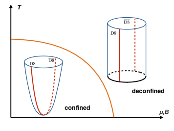
Figure 5: The critical temperature of Hawking-Page transition as the temperature of QCD deconfinement transition in the D4/D8 model with chemical potential $\mu$ or magnetic field $B$.

$$F_{\mathrm{conf.}} =-\frac{2N_{c}^{2}M_{KK}^{4}\lambda V_{4}}{3^{7}\pi^{2}}\left[1-\frac{48}{7}\epsilon_{f}\frac{\pi^{3/2}}{\Gamma\left(-2/3\right)\Gamma\left(1/6\right)}\right],$$

$$F_{\mathrm{deconf.}} =-\frac{2^{7}N_{c}^{2}T^{6}\pi^{4}\lambda V_{4}}{3^{7}M_{KK}^{2}}\left[1+\frac{4}{7}\epsilon_{fT}\left(1+\frac{7}{6}q^{2}\right)\right],$$ (3.32)

where

$$\epsilon_{fT}=\frac{R^{3/2}U_{H}^{1/2}g_{s}Q_{f}}{l_{s}^{2}}=\frac{\lambda^{2}}{12\pi^{3}}\frac{2\pi T}{M_{KK}}\frac{N_{f}}{N_{c}}\ll 1,$$ (3.33)

and we have used the choice of the relevant constants given in (3.20). Therefore, compare the free energy given in (3.32), we can obtain the critical temperature with flavors as,

$$\frac{2\pi T_{c}}{M_{KK}}=1-\frac{1}{126\pi^{3}}\lambda^{2}\frac{N_{f}}{N_{c}}\left[1+\frac{12\pi^{3/2}}{\Gamma\left(-2/3\right)\Gamma\left(1/6\right)}\right]-\frac{27}{16\pi}\frac{N_{f}}{N_{c}}\frac{\mu^{2}}{M_{KK}^{2}},$$ (3.34)

where $\mu$ is the chemical potential in the dual theory given by $A_{t}\big{|}_{U\rightarrow\infty}=\mu$. And the behavior of the Hawking-Page transition given in (3.34) agrees qualitatively with the QCD deconfinement transition [79, 80, 81, 82].

Moreover, when the backreaction to the bulk geometry of the flavor branes is picked up, it is also possible to evaluate QCD deconfinement transition under an external magnetic field. Because extremely strong magnetic field may also give rise to deconfinement transition in QCD [83, 84, 85, 86]. The setup follows mostly the same discussion given above while we need to turn on a constant magnetic field in the DBI action presented in (3.8), as the only non-zero component of the gauge field strength. Then we can derive the effective 1d action by using the metric ansatz (3.9) and (3.21) with respect to the bubble and black D4-brane background. Fortunately, it is possible to find an analytical solution, which leads to critical temperature $T_{c}$ as

$$\frac{2\pi T_{c}}{M_{KK}}=1+\frac{N_{f}}{N_{c}}\left(X\lambda^{2}+\frac{B^{2}}{M_{KK}^{4}}Y\right),$$ (3.35)

by comparing free energy in the same way. Here $B$ refers to the external magnetic field, and $X,Y$ are numerical numbers. For the probe approximation limit of the D8-brane, $X,Y$ are calculated as,

$$X =-\frac{1}{126\pi^{3}}\left[1-\frac{8\pi^{3/2}}{3\Gamma\left(1/6\right)\Gamma\left(4/3\right)}\right]\simeq 5\times 10^{-4},$$

$$Y =-\frac{81}{16\pi}\left[1-\frac{2\pi^{3/2}}{3\Gamma\left(1/6\right)\Gamma\left(4/3\right)}\right]\simeq-0.408.$$ (3.36)

By considering the backreaction of the D8-branes, $X,Y$ are calculated as,

$$X\simeq 5\times 10^{-4},Y\simeq-2.44.$$ (3.37)

And the behavior of the critical temperature illustrated in (3.35) also coincides qualitatively with the QCD deconfinement transition under external magnetic field predicted by lattice QCD [83]. We plot out the behavior of the critical temperature given in (3.34) and (3.35) in Figure 5. In this sense, we could conclude at least, investigating the Hawking-Page transition in the D4/D8 model is very suggestive to study the QCD deconfinement transition in holography which also covers partly the discussion in some bottom-up approaches [87, 88].

3.2 Phase diagram with chiral transition

As we have reviewed the deconfinement transition in the D4/D8 model which can not be distinguished from the chiral transition, let us focus on the chiral transition in the D4/D8 model since QCD has various phases with chiral symmetry.

Recall the relation of $\mathrm{D8/\overline{D8}}$-brane configuration and chiral symmetry, the chiral transition is identified as the transition from connected to disconnected configuration of the $\mathrm{D8/\overline{D8}}$-branes. Hence we need to choose the black D4-brane background in order to include both the connected and disconnected $\mathrm{D8/\overline{D8}}$-brane configuration. The main idea to evaluate the phase transition follows the Section 3.1, which is to compute the free energy in holography. As we will work with respect to the black D4-brane background only, the contribution from the bulk geometry would be irrelevant, because the difference of the free energy determines the phase transition. Keeping this in mind, we can quickly write down the D8-brane action for mesonic (broken chiral symmetry) and quark matter phase (restored chiral symmetry) with a $U\left(1\right)$ chemical potential $\hat{A}_{0}$, which corresponds to the connected and disconnected D8-brane configuration respectively in Figure 3 as,

$$S_{\mathrm{DBI}}^{\mathrm{D8}}=\mathcal{N}\frac{V_{3}}{T}\int_{u_{0}}^{\infty}duu^{5/2}\sqrt{1+u^{3}f_{T}\left(x_{4}^{\prime}\right)^{2}-\hat{a}_{0}^{\prime 2}},$$ (3.38)

where the variables in (3.38) are dimensionless as,

$$x_{4}=x^{4}M_{KK},u=\frac{U}{R}\frac{1}{\left(M_{KK}R\right)^{2}},\hat{a}_{0}=\hat{A}_{0}\frac{4\pi}{\lambda M_{KK}},\mathcal{N}=2T_{\mathrm{D8}}\Omega_{4}R^{5}\left(M_{KK}R\right)^{7}.$$ (3.39)

The equation of motion can be obtained by varying (3.38) respected to $x_{4}$ and $\hat{a}_{0}$ which are,

$$\frac{u^{5/2}\hat{a}_{0}^{\prime}}{\sqrt{1+u^{3}f_{T}x_{4}^{\prime 2}-\hat{a}_{0}^{\prime 2}}} =n_{I},$$

$$\frac{u^{11/2}f_{T}x_{4}^{\prime}}{\sqrt{1+u^{3}f_{T}x_{4}^{\prime 2}-\hat{a}_{0}^{\prime 2}}} =f_{T}^{1/2}\left(u_{0}\right)u_{0}^{4},$$ (3.40)

where “$\prime$” refers to the derivative with respect to $u$. The constant $n_{I}$ corresponds to the $U\left(1\right)$ charge density which is therefore the baryon number in this setup. In the mesonic phase, the baryon number is zero i.e. $n_{I}=0$, and the equations of motion in (3.40) can be solved by the following boundary condition according to the connected configuration in Figure 3, as

$$\hat{a}_{0}^{\prime}\left(u_{0}\right) =0,\ \hat{a}_{0}\left(\infty\right)=\mu,$$

$$x_{4}^{\prime}\left(u_{0}\right) =\infty,\ \frac{l}{2}=\int_{u_{0}}^{\infty}dux_{4}^{\prime},$$ (3.41)

where constant $\mu$ refers to the chemical potential in the dual theory, constant $l$ refers to the separation of the $\mathrm{D8/\overline{D8}}$-branes at boundary $u\rightarrow\infty$. Thus the solution is

$$\hat{a}_{0}=\mu,x_{4}^{\prime}=\frac{f_{T}^{1/2}\left(u_{0}\right)u_{0}^{4}}{f_{T}^{1/2}\left(u\right)u^{3/2}\sqrt{u^{8}f_{T}\left(u\right)-u_{0}^{8}f_{T}\left(u_{0}\right)}}.$$ (3.42)

Put the solution (3.42) back into action (3.38), we can obtain the free energy as,

$$F_{\mathrm{mesonic}}=\mathcal{N}\int_{u_{0}}^{\infty}duu^{5/2}\frac{u^{4}f_{T}^{1/2}\left(u\right)}{\sqrt{u^{8}f_{T}\left(u\right)-u_{0}^{8}f_{T}\left(u_{0}\right)}}.$$ (3.43)

For the quark matter phase, the boundary condition reads from the disconnected configuration in Figure 3 as,

$$\hat{a}_{0}\left(u_{H}\right)=0,\hat{a}_{0}\left(\infty\right)=\mu,x_{4}^{\prime}=0,$$ (3.44)

which leads to a solution with hyper geometrical functions as,

$$\hat{a}_{0}\left(u\right)=\mu-\frac{n_{I}^{2/5}\Gamma\left(3/10\right)\Gamma\left(6/5\right)}{\sqrt{\pi}}+u\ _{2}F_{1}\left(\frac{1}{5},\frac{1}{2},\frac{6}{5},-\frac{u^{5}}{n_{I}^{2}}\right).$$ (3.45)

Therefore the free energy is computed as,

$$F_{\mathrm{quarkmatter}}=\mathcal{N}\int_{u_{H}}^{\infty}du\frac{u^{5}}{\sqrt{u^{5}+n_{I}^{5}}}.$$ (3.46)

We note that the condition $\hat{a}_{0}\left(u_{H}\right)=0$ implies $n_{I}$ is a function of $\mu$ as,

$$0=\mu-\frac{n_{I}^{2/5}\Gamma\left(3/10\right)\Gamma\left(6/5\right)}{\sqrt{\pi}}+u_{H}\ {}_{2}F_{1}\left(\frac{1}{5},\frac{1}{2},\frac{6}{5},-\frac{u_{H}^{5}}{n_{I}^{2}}\right).$$ (3.47)

Then the phase diagram can be obtained by compare the free energy given in (3.43) and (3.47) with constraint (3.46). Notice that while the free energy given in (3.43) and (3.47) is divergent, their difference which determines the phase diagram remains to be finite. Thus it is not necessary to do the holographic renormalization in this case.

For a more ambitious approach, let us include the baryonic phase in the black D4-brane background, that is to take into account the configuration (c) in Figure 4 which has broken chiral symmetry with baryon vertex. Since baryon vertex is identified as $\mathrm{D4}^{\prime}$-brane described equivalently by instantons on the D8-branes, we employ the BPST instanton solution given in (2.85) to represent baryon on the flavor brane. For multiple baryons we can summarize the instanton field strength as what we have discussed in Section 2.5, in this sense baryons are treated as instanton gas on the flavor brane. On the other hand, as the instanton size takes order of $\lambda^{-1/2}$ and the DBI action (2.20) does not define how to treat it with non-Abelian gauge field, we may generalize the DBI action by taking all order of gauge field strength into non-Abelian case through the identity for Abelian gauge field strength $\hat{F}$ as,

$$\sqrt{\det\left(g+2\pi\alpha^{\prime}\hat{F}\right)}= U^{4}\left(\frac{R}{U}\right)^{3/4}\big{\{}\left(2\pi\alpha^{\prime}\right)^{2}f_{T}\hat{F}_{iU}^{2}+\left(1+u^{3}f_{T}x_{4}^{\prime 2}-\hat{a}_{0}^{\prime 2}\right)\left[1+\left(\frac{R}{U}\right)^{3}\frac{\left(2\pi\alpha^{\prime}\right)^{2}}{2}\hat{F}_{ij}^{2}\right]$$

$$+\left(\frac{R}{U}\right)^{3}\frac{\left(2\pi\alpha^{\prime}\right)^{4}f_{T}\left(\hat{F}_{ij}\hat{F}_{kU}\epsilon_{ijk}\right)^{2}}{4}\big{\}}^{1/2}.$$ (3.48)

For non-Abelian generalization, we follow [90] to replace the quadratic terms of $\hat{F}$ by its non-Abelian version $F$ then take trace of each term separately as,

$$\hat{F}_{iU}^{2}\rightarrow\mathrm{Tr}F_{iU}^{2},\hat{F}_{ij}^{2}\rightarrow\mathrm{Tr}F_{ij}^{2},\hat{F}_{ij}\hat{F}_{kU}\rightarrow\mathrm{Tr}F_{ij}F_{kU}.$$ (3.49)

Afterwards we impose the BPST instanton solution (2.85) with multiple number $n_{I}$ to $F$ in order to represent baryons . Altogether, we reach to a generalized version of action for baryonic phase as,

$$F_{\mathrm{baryonic}}=S^{\mathrm{D8}}=\mathcal{N}\frac{V_{3}}{T}\int_{u_{c}}^{\infty}\left[\sqrt{\left(1+g_{1}+u^{3}f_{T}x_{4}^{\prime 2}-\hat{a}_{0}^{\prime 2}\right)\left(1+g_{2}\right)}-n_{I}\hat{a}_{0}\left(u\right)q\left(u\right)\right],$$ (3.50)

where

$$g_{1}\left(u\right) =\frac{f_{T}\left(u\right)u^{1/2}}{3u_{c}^{2}\sqrt{f_{c}\left(u\right)}}n_{I}q\left(u\right),f_{c}\left(u\right)=1-\frac{u_{c}^{3}}{u^{3}},$$

$$g_{2}\left(u\right) =\frac{u_{c}^{2}\sqrt{f_{c}\left(u\right)}}{3u^{7/2}}n_{I}q\left(u\right),q\left(Z\right)=\frac{3\rho^{4}}{4\left(Z^{2}+\rho^{2}\right)^{5/2}}.$$ (3.51)

We note that the last term in (3.50) is the Chern-Simons action and $q\left(Z\right)$ is the average instanton field strength defined by the summary of the BPST instanton (2.85) as [91]

$$\frac{1}{V_{3}}\sum_{n=1}^{N_{I}}\int d^{3}X\frac{4\left(\rho/\gamma\right)^{4}}{\left[\left(\vec{X}-\vec{X}_{0n}\right)^{2}+\left(Z/\gamma\right)^{2}+\left(\rho/\gamma\right)^{2}\right]^{4}}=\frac{2}{3}\pi^{2}\gamma q\left(Z\right)n_{I},$$ (3.52)

with normalization condition

$$\int_{-\infty}^{+\infty}q\left(Z\right)dZ=1.$$ (3.53)

$\vec{X}_{0n}$ refers to the center of the $n$-th instanton. $Z$ is the Cartesian coordinate, in the case of (c) in Figure 4, it is defined as,

$$U^{3}=U_{c}^{3}+U_{c}Z^{2},$$ (3.54)

where we use $U_{c}$ to denote the connected position of $\mathrm{D8/\overline{D8}}$-branes with instantons to distinguish it from $U_{0}$ in which instantons are absent. $N_{I}$ is the instanton number which relates to its number density $n_{I}$ as $n_{I}=N_{I}96\pi^{4}/\left(\lambda^{2}M_{KK}^{3}\right)$. With the boundary condition

$$\frac{l}{2}=\int_{u_{c}}^{\infty}dux_{4}^{\prime},\hat{a}_{0}\left(\infty\right)=\mu,$$ (3.55)

the equations of motion obtained by varying (3.50),

$$\frac{u^{5/2}\hat{a}_{0}^{\prime}\sqrt{1+g_{2}}}{\sqrt{1+g_{1}+u^{3}f_{T}x_{4}^{\prime 2}-\hat{a}_{0}^{\prime 2}}} =n_{I}Q$$

$$\frac{u^{11/2}f_{T}x_{4}^{\prime}\sqrt{1+g_{2}}}{\sqrt{1+g_{1}+u^{3}f_{T}x_{4}^{\prime 2}-\hat{a}_{0}^{\prime 2}}} =k,$$ (3.56)

where $k$ is an integration constant to be determined and

$$Q\left(u\right)=\int_{u_{c}}^{u}q\left(v\right)dv=\frac{u^{3/2}\sqrt{f_{c}}}{2}\frac{3\rho^{2}u_{c}+2\left(u^{3}-u_{c}^{3}\right)}{\left(u^{3}-u_{c}^{3}+\rho^{2}u_{c}\right)^{3/2}},$$ (3.57)

can be solved as,

$$\hat{a}_{0}^{\prime 2} =\frac{\left(n_{I}Q\right)^{2}}{u^{5}}\frac{1+g_{1}}{1+g_{2}-\frac{k^{2}}{u^{8}f_{T}}+\frac{\left(n_{I}Q\right)^{2}}{u^{5}}},$$

$$x_{4}^{\prime 2} =\frac{k^{2}}{u^{11}f_{T}^{2}}\frac{1+g_{1}}{1+g_{2}-\frac{k^{2}}{u^{8}f_{T}}+\frac{\left(n_{I}Q\right)^{2}}{u^{5}}}.$$ (3.58)

Plugging solution (3.58) back into (3.50), we can obtain the free energy of the baryonic phase. In order to obtain the phase transition, we need to further minimize the free energy given in (3.50) with respect to $n_{I},\rho,u_{c}$ as the parameters which leads to three constraints as,

$$0= \int_{u_{c}}^{\infty}\left[\frac{u^{5/2}}{2}\left(\frac{\partial g_{1}}{\partial n_{I}}\zeta^{-1}+\frac{\partial g_{2}}{\partial n_{I}}\zeta\right)+\hat{a}_{0}^{\prime}Q\right]-\mu,$$

$$0= \int_{u_{c}}^{\infty}\left[\frac{u^{5/2}}{2}\left(\frac{\partial g_{1}}{\partial\rho}\zeta^{-1}+\frac{\partial g_{2}}{\partial\rho}\zeta\right)+n_{I}\hat{a}_{0}^{\prime}\frac{\partial Q}{\partial\rho}\right],$$

$$u_{c}^{5/2}\sqrt{\left[1+g_{1}\left(u_{c}\right)\right]\left[1+g_{2}\left(u_{c}\right)-\frac{k^{2}}{u_{c}^{8}f_{T}\left(u_{c}\right)}\right]}= \int_{u_{c}}^{\infty}\left[\frac{u^{5/2}}{2}\left(\frac{\partial g_{1}}{\partial u_{c}}\zeta^{-1}+\frac{\partial g_{2}}{\partial u_{c}}\zeta\right)+n_{I}\hat{a}_{0}^{\prime}\frac{\partial Q}{\partial u_{c}}\right],$$ (3.59)

where

$$\zeta=\frac{\sqrt{1+g_{1}}}{\sqrt{1+g_{2}-\frac{k^{2}}{u^{8}f_{T}}+\frac{\left(n_{I}Q\right)^{2}}{u^{5}}}}.$$ (3.60)

With all above in hand, we can obtain numerically a holographic diagram included mesonic, baryonic and quark matter phase of QCD by comparing the associated free energies given in (3.43) (3.46) and (3.50). The resultant phase diagram is given in Figure 6.

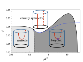
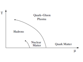
Figure 6: Holographic QCD phase diagram vs realistic QCD phase diagram in the $T-\mu$ plane.

and we can see the holographic diagram includes all the elementary phases in realistic QCD although the confined geometry is not included in the current discussion.

We note that it is very difficult to work out a reasonable model describing QCD matter over a very wide density regime with traditional models or theories of QCD. For example, the quark-meson model (e.g. [92, 93]) and the Nambu-Jona-Lasinio (NJL) model [94, 95, 96, 97, 98] are very useful to get some insight into the chiral and deconfinement phase transitions and quark matter phases, however the nuclear matter is usually not included in these models. In addition, nucleon-meson models e.g. [99, 100, 101, 102] are based on the properties of nuclear matter and may be able to describe moderately dense nuclear matter realistically, while they give a poor description of quark matter with restored chiral symmetry. In this sense, this holographic model provides a very powerful way to study QCD phase diagram in a very wide density regime based on string theory.

3.3 Higgs mechanism and heavy-light meson field

One of the interesting developments of the D4/D8 model is to include heavy flavor by using the Higgs mechanism in D-brane system. Recall that the fundamental quarks in the D4/D8 model are identified to be the $4-8$ and $4-\bar{8}$ strings. Since $N_{c}$ D4-branes and $N_{f}$ D8-branes are coincident, we find that the $4-8$ and $4-\bar{8}$ strings have a vanishing vacuum expectation value (VEV). Therefore the fundamental quarks created by $4-8$ and $4-\bar{8}$ strings are massless which implies this model can describe the mesons with light flavors only. Hence it is naturally motivated to include the massive heavy flavor in this model. To this goal, in this section, let us review the Higgs mechanism in D-brane system and see how to use it to introduce heavy flavor.

First, we take a look at the Higgs mechanism in D-brane system by considering the configuration of an open string connecting two stacks of the separated D-branes as it is illustrated in (a) of Figure 7.

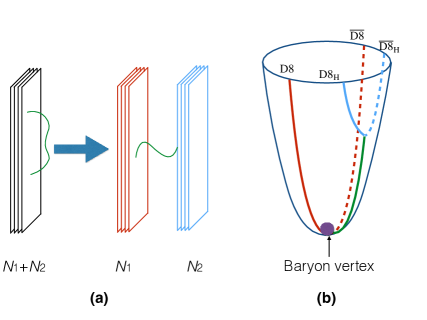
Figure 7: The Higgs mechanism in string theory (a) and the configuration of heavy flavor in D4/D8 model (b). (a) Higgs mechanism in string theory: The gauge symmetry on a stack of coincident $N_{1}+N_{2}$ D-branes could be $U\left(N_{1}+N_{2}\right)$, while it breaks down to $U\left(N_{1}\right)\times U\left(N_{2}\right)$ if the D-branes somehow move apart to become two stacks of coincident $N_{1}$ and $N_{2}$ D-branes. The open string connecting the two stacks of the D-branes has a non-zero VEV hence its ground states acquire non-zero mass which corresponds to the separation of the D-branes. (b) Configuration of heavy flavor in D4/D8 model: Red line refers to the stack of $N_{f}$ $\mathrm{D8/\overline{D8}}$-branes in the original model which now is identified as light flavor. Blue line refers to another one pair of $\mathrm{D8/\overline{D8}}$-branes separated from $N_{f}$ $\mathrm{D8/\overline{D8}}$-branes which is identified as heavy flavor. The green line refers to the open string connecting the light and heavy brane which is the heavy-light string, and it acquires non-zero VEV to create massive ground states.

In this D-brane configuration, the worldvolume symmetry $U\left(N_{1}+N_{2}\right)$ breaks down to $U\left(N_{1}\right)\times U\left(N_{2}\right)$ when the D-branes move separately, where we use $N_{1},N_{2}$ to refer to the D-branes number in each stack. Accordingly the transverse modes of the D-brane acquire a non-zero VEV due to the separation of the D-branes. Hence the multiplets created by the open string connecting the separated D-branes become massive just like the Higgs mechanism in the standard model of the particle physics [53, 60]. Let us investigate this mechanism quantitatively by recalling the D-brane action in (2.20). In the holographic approach, we need the near-horizon limit i.e. $\alpha^{\prime}\rightarrow 0$, thus the D-brane action can be expanded to be Yang-Mills plus Wess-Zumino action as it is in Section 2.4. Now we pick up the transverse modes in the DBI action, it reduces to an additional quadratic action for the transverse modes $\Psi^{I}$ with $\alpha^{\prime}\rightarrow 0$ as,

$$S\left[\Psi^{I}\right] =-T_{\mathrm{D}_{p}}\frac{\left(2\pi\alpha^{\prime}\right)^{2}}{4}\int_{\mathrm{D}_{p}}d^{p+1}x\sqrt{-\det g}e^{-\phi}\mathrm{Tr}\left\{2D_{a}\Psi^{I}D_{a}\Psi^{I}+\left[\Psi^{I},\Psi^{J}\right]^{2}\right\},$$

$$a =0,1...p,\ I,J=p+1...d,$$ (3.61)

where the covariant derivative is

$$D_{a}\Psi^{I}=\partial_{a}\Psi^{I}+i\left[\mathbf{A}_{a},\Psi^{I}\right],$$ (3.62)

and $\mathbf{A}_{a}$ is the gauge field potential on the D-brane. Consider a stack of coincident $N_{1}+N_{2}$ D-branes, $\mathbf{A}_{a}$ could be the $U\left(N_{1}+N_{2}\right)$ generator as an $\left(N_{1}+N_{2}\right)\times\left(N_{1}+N_{2}\right)$ matrix. However, if the coincident $N_{1}+N_{2}$ D-branes move apart to become two stacks of $N_{1}$ and $N_{2}$ D-branes, the gauge potential $\mathbf{A}_{a}$ becomes,

$$\mathbf{A}_{a}=\left(\begin{array}[]{cc}A_{a}&\Phi_{a}\\ \Phi_{a}^{\dagger}&0\end{array}\right),$$ (3.63)

where $A_{a}$ is the $U\left(N_{1}\right)$ gauge potential as an $N_{1}\times N_{1}$ matrix. $\Phi_{a}$ is the multiplet created by the open string connecting to the two stacks of the D-brane which is an $N_{1}\times N_{2}$ matrix-valued field and the last element can be gauged away by the residual symmetry. On the other hand, when the D-branes are separated, the transverse mode $\Psi^{I}$ will have a non-zero VEV since the open string connecting the separated D-branes can not shrink to zero. Therefore we can write down $\Psi^{I}$ with a VEV as,

$$\Psi^{I}\rightarrow\Psi^{I}+V^{I},$$ (3.64)

where

$$V^{I}\sim\left(\begin{array}[]{cc}V&0\\ 0&v\end{array}\right),$$ (3.65)

to represent $U\left(N_{1}+N_{2}\right)\rightarrow U\left(N_{1}\right)\times U\left(N_{2}\right)$. Thus plugging (3.62) - (3.65) into (3.61), one obtains a mass term in the action as

$$\mathrm{Tr}\left(V^{2}\Phi_{a}^{\dagger}\Phi_{a}+v^{2}\Phi_{a}\Phi_{a}^{\dagger}\right),$$ (3.66)

and $\Phi_{a}$ can be interpreted as the heavy-light field acquiring a mass through the VEV of the transverse mode $\Psi^{I}$.

With this Higgs mechanism in string theory, let us employ it in the D4/D8 model by considering (b) of Figure 7. In this configuration, there is one pair of $\mathrm{D8/\overline{D8}}$-branes separated from $N_{f}$ $\mathrm{D8/\overline{D8}}$-branes which is identified as heavy flavor brane with an open string (the heavy-light string) connecting them. We note that the configuration in (b) of Figure 7 is generalized version of (a) of Figure 7 in the curved spacetime. Then we can write down the D8-brane action with heavy flavor by imposing the following replacement,

$$A_{a}\rightarrow\mathbf{A}_{a}=\left(\begin{array}[]{cc}A_{a}&\Phi_{a}\\ \Phi_{a}^{\dagger}&0\end{array}\right),F_{ab}\rightarrow\bm{\mathrm{F}}_{ab}=\left(\begin{array}[]{cc}F_{ab}+i\alpha_{ab}&f_{ab}\\ f_{ab}^{\dagger}&i\beta_{ab}\end{array}\right),$$ (3.67)

to (2.33), where $A_{a},F_{ab}$ are $N_{f}\times N_{f}$ matrix-valued fields as we have specified Section 2. $\Phi_{a}$ is an $N_{f}\times 1$ matrix-valued multiplet created by the heavy-light string which is interpreted as the heavy-light meson field and

$$\alpha_{ab}= 2\Phi_{[a}\Phi_{b]}^{\dagger},\ \beta_{ab}=2\Phi_{[a}^{\dagger}\Phi_{b]},$$

$$f_{ab}= 2\partial_{[a}\Phi_{b]}+2iA_{[a}\Phi_{b]}\equiv 2D_{[a}\Phi_{b]},$$ (3.68)

we obtain the action (3.61) for $\Phi_{a}$ as

$$S\left[\Phi_{\mu,z}\right]= -2\kappa\mathrm{Tr}\int dzdx^{4}f\left(z\right)\left(\partial_{\mu}\Phi_{\nu}^{\dagger}-\partial_{\nu}\Phi_{\mu}^{\dagger}\right)\left(\partial^{\mu}\Phi^{\nu}-\partial^{\nu}\Phi^{\mu}\right)$$

$$-\kappa\mathrm{Tr}\int dzdx^{4}g\left(z\right)\left(\partial_{\mu}\Phi_{z}^{\dagger}-\partial_{z}\Phi_{\mu}^{\dagger}\right)\left(\partial^{\mu}\Phi_{z}-\partial_{z}\Phi^{\mu}\right)$$

$$-\tilde{v}\mathrm{Tr}\int dzdx^{4}a\left(z\right)\left[2f\left(z\right)\Phi^{\dagger\mu}\Phi_{\mu}+g\left(z\right)\Phi_{z}^{\dagger}\Phi_{z}\right],$$ (3.69)

where $z$ is the Cartesian coordinates given in (2.34) and the VEV of T-dualitied $\Psi^{4}=2\pi\alpha^{\prime}x^{4}$ is chosen as [103],

$$\Psi^{4}=\left(\begin{array}[]{cc}-\frac{v}{N_{f}-1}\mathbf{1}_{N_{f}-1}&0\\ 0&v\end{array}\right),$$ (3.70)

with

$$\tilde{v}=v\kappa/\left(2\pi\alpha^{\prime}\right)^{2},f\left(z\right)=\frac{R^{3}}{4U\left(z\right)},g\left(z\right)=\frac{9}{8}\frac{U\left(z\right)^{3}}{U_{KK}},a\left(z\right)=\left[\frac{U\left(z\right)}{R}\right]^{3/2}.$$ (3.71)

Note that $\Psi^{4}$ is the only transverse mode of D8-brane. The heavy-light meson tower can be obtained by expanding $\Phi_{\mu,z}$ as what we have specified in Section 2.4. For example, the transverse modes of heavy-light meson field is suggested as [38, 39],

$$\Phi_{\mu}=\sum_{n}\phi_{\left(n\right)}^{H}\left(z\right)B_{\mu}^{\left(n\right)}\left(x\right),\Phi_{z}=0,$$ (3.72)

which leads to

$$S\left[\Phi_{\mu,z}\right]=\sum_{n}\int d^{4}x\left[\frac{1}{2}\partial_{[\mu}B_{\nu]}^{\left(n\right)\dagger}\partial^{[\mu}B^{\left(n\right)\nu]}+m_{n}^{2}B_{\mu}^{\left(n\right)\dagger}B^{\left(n\right)\mu}\right],$$ (3.73)

with the normalization

$$4\kappa\int dzf\left(z\right)\phi_{\left(n\right)}^{H}\phi_{\left(m\right)}^{H}=\delta_{mn},$$ (3.74)

and eigenvalue equation,

$$-\frac{d}{dz}\left(g\frac{d\phi_{\left(n\right)}^{H}}{dz}\right)+2f\left(z\right)\left[-m_{n}^{2}+\tilde{v}^{2}a\left(z\right)\right]\phi_{n}^{H}=0.$$ (3.75)

For the transverse modes longitudinal modes, the expansion is suggested as,

$$\Phi_{\mu}= -\sum_{n}\frac{1}{2a\left(z\right)f\left(z\right)m_{n}^{2}}\frac{d}{dz}\left[a\left(z\right)g\left(z\right)\epsilon_{n}\left(z\right)\right]\partial_{\mu}D_{\nu}\left(x\right),$$

$$\Phi_{z}= \sum_{n}\epsilon_{n}\left(z\right)D_{n}\left(x\right),$$ (3.76)

leading to

$$S\left[\Phi_{\mu,z}\right]=\sum_{n}\int d^{4}x\left(\partial_{\mu}D_{n}^{\dagger}\partial^{\mu}D_{n}+m_{n}^{2}D_{n}^{\dagger}D_{n}\right),$$ (3.77)

with the normalization

$$2\kappa=\int dza\left(z\right)g\left(z\right)\epsilon_{n}\left(z\right)\epsilon_{m}\left(z\right)=\frac{m_{n}^{2}}{\tilde{v}^{2}}\delta_{mn}.$$ (3.78)

We note that, with the replacement (3.67), the Chern-Simons action (2.57) for the D8-branes reduces to additional terms as,

$$\mathcal{L}_{\mathrm{CS}}\left[\Phi_{\mu,z}\right]= -\frac{N_{c}}{24\pi^{2}}\left(d\Phi^{\dagger}Ad\Phi+d\Phi^{\dagger}dA\Phi+\Phi^{\dagger}dAd\Phi\right)$$

$$+\frac{iN_{c}}{16\pi^{2}}\left(d\Phi^{\dagger}A^{2}\Phi+\Phi^{\dagger}A^{2}d\Phi+\Phi^{\dagger}AdA\Phi+\Phi^{\dagger}dAA\Phi\right)$$

$$+\frac{5N_{c}}{48\pi^{2}}\Phi^{\dagger}A^{3}\Phi+\mathcal{O}\left(\Phi^{4},A\right).$$ (3.79)

Using the expansion (3.72) (3.76) and (2.46), the DBI and CS term includes the interaction between light and heavy-light mesons.

It is also possible to obtain the baryon spectrum with heavy flavor by considering baryon vertex as the instantons on the flavor brane [104, 105, 106]. Follow the steps in Section 2.5, the equations of motion for the heavy-light meson field is derived as,

$$D_{M}D_{M}\Phi_{N}-D_{N}D_{M}\Phi_{M}+2iF_{MN}\Phi_{M}+\mathcal{O}\left(\lambda^{-1}\right) =0,$$

$$D_{M}\left(D_{0}\Phi_{M}-D_{M}\Phi_{0}\right)-iF^{0M}\Phi_{M}$$

$$-\frac{1}{64\pi^{2}a}\epsilon_{MNPQ}\mathcal{K}_{MNPQ}+\mathcal{O}\left(\lambda^{-1}\right) =0,$$ (3.80)

with $M,N=1,2,3,z$ and

$$\mathcal{K}_{MNPQ}=i\partial_{M}A_{N}\partial_{P}\Phi_{Q}-A_{M}A_{N}\partial_{P}\Phi_{Q}-\partial_{M}A_{N}A_{P}\Phi_{Q}-\frac{5i}{6}A_{M}A_{N}A_{P}\Phi_{Q},$$ (3.81)

where $F=dA+\frac{i}{2}\left[A,A\right]$ is computed by the BPST instanton solution given in (2.82) - (2.87). Thus $\Phi_{\mu,z}$ can be solved as $\Phi_{\mu,z}=e^{\pm im_{H}t}\phi_{\mu,z}\left(x\right)$ by

$$\phi_{0} =-\frac{1}{1024a\pi^{2}}\left[\frac{25\rho}{2\left(x^{2}+\rho^{2}\right)^{5/2}}+\frac{7}{\rho\left(x^{2}+\rho^{2}\right)^{3/2}}\right]\chi,$$

$$\phi_{M} =\frac{\rho}{\left(x^{2}+\rho^{2}\right)^{3/2}}\sigma_{M}\chi,$$ (3.82)

where $\sigma_{M}$ is the embedded Pauli matrices as $\sigma_{M}/2=\left(t_{i},-\mathbf{1}_{N_{f}}\right)$ and $\chi$ is the $SU\left(N_{f}\right)$ spinor independent on $x,z$. The soliton mass as the baryonic potential can be evaluated by inserting (3.82) and the BPST solution (2.82) - (2.87) to the full action for the D8-branes. Afterwards one reaches to an effective Hamiltonian for baryon state by following Section 2.5 as it is given in [105, 106]. We note that [40] also gives another generalization with heavy flavor into black D4-brane background.

3.4 Interaction of hadron and glueball

The interaction of hadrons relates to many significant topics in QCD and nuclear physics, and its holographic description by the D4/D8 model has been reviewed briefly in Section 2 and [24, 25]. In this section, we will take a look at the interaction in hadron physics involving glueballs since the D4/D8 model provides explicit definition of meson, baryon and glueball.

The main idea to include the interaction of meson and glueball is to consider the D8-brane action with a gravitational fluctuation. Recall the discussion in Section 2.4 and 2.6, since meson is identified as the gauge field on the D8-branes (created by $8-8$ string) and glueball is identified as the gravitational polarization (close string), the interaction of meson and glueball is nothing but the interaction of open and close string which can be therefore included into the D8-brane action when the metric fluctuation is picked up. For example, when we put the gravitational polarization (2.99) into the D8-brane action (2.32) with the meson tower given in (2.37), by integrating out the $z$ dependence (the holographic coordinate) it reduces to interaction action involving $\pi,\rho$ meson and exotic glueball $G_{E}$ after some straightforward but messy calculations as,

$$S_{G_{E}}^{\pi-\rho}= -\mathrm{Tr}\int d^{4}x\bigg{\{}c_{1}\left[\frac{1}{2}\partial_{\mu}\pi\partial_{\nu}\pi\frac{\partial^{\mu}\partial^{\nu}}{M_{E}^{2}}G_{E}+\frac{1}{4}\left(\partial_{\mu}\pi\right)^{2}\left(1-\frac{\partial^{2}}{M_{E}^{2}}\right)G_{E}\right]$$

$$+c_{2}M_{KK}^{2}\left[\frac{1}{2}\rho_{\mu}\rho_{\nu}\frac{\partial^{\mu}\partial^{\nu}}{M_{E}^{2}}G_{E}+\frac{1}{4}\left(\rho_{\mu}\right)^{2}\left(1-\frac{\partial^{2}}{M_{E}^{2}}\right)G_{E}\right]$$

$$+c_{3}\left[\frac{1}{2}\eta^{\sigma\lambda}\partial_{[\mu}\rho_{\sigma]}\partial_{[\nu}\rho_{\lambda]}\frac{\partial^{\mu}\partial^{\nu}}{M_{E}^{2}}G_{E}-\frac{1}{8}\partial_{[\mu}\rho_{\nu]}\partial^{[\mu}\rho^{\nu]}\left(1+\frac{\partial^{2}}{M_{E}^{2}}\right)G_{E}\right]+c_{4}\frac{3}{2M_{E}^{2}}\rho_{\mu}\partial^{[\mu}\rho^{\nu]}\partial_{\nu}G_{E}$$

$$+c_{5}\left[\partial_{\mu}\pi\left[\pi,\rho_{\nu}\right]\frac{\partial^{\mu}\partial^{\nu}}{M_{E}^{2}}G_{E}+\frac{1}{2}\partial_{\mu}\pi\left[\pi,\rho^{\mu}\right]\left(1-\frac{\partial^{2}}{M_{E}^{2}}\right)G_{E}\right]$$

$$+\left[\frac{1}{2}\tilde{c}_{1}\left(\partial_{\mu}\pi\right)^{2}+\frac{1}{2}\tilde{c}_{2}M_{KK}^{2}\left(\rho_{\mu}\right)^{2}+\frac{1}{4}\tilde{c}_{3}\partial_{[\mu}\rho_{\nu]}\partial^{[\mu}\rho^{\nu]}+\tilde{c}_{5}\partial_{\mu}\pi\left[\pi,\rho^{\mu}\right]\right]G_{E}\bigg{\}},$$ (3.83)

where the coefficients $c_{i}$’s and $\tilde{c}_{i}$’s are coupling constants and numerically computed as (in the unit of $\lambda^{-1/2}N_{c}^{-1}M_{KK}^{-1}$),

$$c_{1} =\int dZ\frac{\bar{H}_{E}}{\pi K}=62.6,\ \ \ \ c_{2}=2\kappa\int dZK\left(\psi_{1}^{\prime}\right)\bar{H}_{E}=7.1,$$

$$c_{3} =2\kappa\int dZK^{-1/3}\left(\psi_{1}\right)^{2}\bar{H}_{E}=69.7,$$

$$c_{4} =2\kappa M_{KK}^{2}\int dZ\frac{20ZK}{\left(5K-2\right)^{2}}\psi_{1}\psi_{1}^{\prime}H_{E}=10.6M_{KK}^{2},$$

$$c_{5} =\int dZ\frac{\psi_{1}\bar{H}_{E}}{\pi K}=2019.6N_{c}^{-1/2},$$

$$\tilde{c}_{1} =\int dZ\frac{H_{E}}{4\pi K}=16.4,\ \ \ \ \tilde{c}_{2}=\frac{1}{2}\kappa\int dZK\left(\psi_{1}^{\prime}\right)^{2}H_{E}=3.0,$$

$$\tilde{c}_{3} =\frac{1}{2}\kappa\int dZK^{-1/3}\left(\psi_{1}\right)^{2}H_{E}=18.1,\ \ \ \ \tilde{c}_{5}=\int dZ\frac{\psi_{1}H_{E}}{4\pi K}=508.2N_{c}^{-1/2}.$$ (3.84)

Then the associated amplitude of glueball decay can be further evaluated by using the effective action $S_{G_{E}}^{\pi-\rho}$ with the coupling constants. And one can also compute the effective action of meson involving other types of glueball by changing the formulas of the bulk gravitational polarization as it is discussed in [29, 30, 31, 32].

The current setup to obtain an effective action of meson and glueball interaction can also be generalized by including heavy flavor [107] which is to take into account the configuration (b) in Figure 7 and the heavy-light meson field. The main idea is to pick up the gravitational polarization in bulk metric when we write down the D8-brane action with heavy flavor brane (i.e. with the replacement given in (3.67)). For example, by considering the gravitational polarization for the exotic glueball $G_{E}$ in (2.99), the effective action of heavy-light meson and glueball provides terms as,

$$\partial^{2}G_{E}\partial_{\mu}Q_{\nu}^{\dagger}\partial^{\mu}Q^{\nu}, \partial^{2}G_{E}Q_{\mu}^{\dagger}Q^{\mu},\partial^{2}G_{E}\partial_{\mu}Q^{\dagger}\partial^{\mu}Q,\partial^{2}G_{E}Q^{\dagger}Q,$$

$$\partial^{\mu}\partial^{\rho}G_{E}\partial_{\mu}Q_{\nu}^{\dagger}\partial_{\rho}Q^{\nu}, \partial^{\mu}\partial^{\nu}G_{E}\partial_{\mu}Q^{\dagger}\partial_{\nu}Q,\partial^{\mu}\partial^{\nu}G_{E}Q_{\mu,}^{\dagger}Q_{\nu,}$$

$$G_{E}\partial_{\mu}Q_{\nu}^{\dagger}\partial^{\mu}Q^{\nu}, G_{E}Q_{\mu}^{\dagger}Q^{\nu},G_{E}Q^{\dagger}Q,$$

$$\partial_{\sigma}G_{E}\partial^{\rho}Q^{\sigma\dagger}\partial_{\rho}Q, \partial_{\sigma}G_{E}\partial^{\rho}Q^{\sigma\dagger}Q_{\rho},\partial^{\mu}G_{E}Q_{\mu}^{\dagger}Q,$$ (3.85)

which are the same types as the interaction given in (3.83). Here we have used $Q_{\mu},Q$ to denote the vector and scalar heavy-light meson field, and the lowest heavy-light meson is identified to be D-meson with a charm quark. Accordingly, the effective action with heavy-flavor and glueball may be useful to study the oscillation of D-meson pairs ($D-\bar{D}$) or B-meson pairs ($B-\bar{B}$) [108, 109]. Note that since the heavy-light multiplet is created by the heavy-light string, even if the heavy flavor is taken into account, the interaction of heavy-light meson and glueball remains to be the open/close string interaction through holography. Besides, in the presence of the heavy-light meson and glueball, the effective action also mixes the interaction terms of glueball, light and heavy-light meson which may describe the various interaction in hadron physics.

It is also possible to include the interaction of baryon (or baryonic meson) and glueball in a parallel way, that is to consider the interaction of baryonic $\mathrm{D4}^{\prime}$-branes and bulk close string [110]. Specifically, one can derive the Yang-Mills action presented in (2.32) with the gravitational polarization (2.99), then insert the BPST instanton configuration (2.82) - (2.87) as baryon under the large $\lambda$ rescaling (2.77). Afterwards, by following the discussion in Section 2.5, we can obtain additional terms to the collective Hamiltonian (2.98) as,

$$\Delta H\left(t\right)\simeq\cos\left(\omega t\right)\left\{-\frac{27}{2}\pi^{2}+\left[-\frac{59049\pi^{4}}{20\rho^{2}}+\frac{27M_{E}^{2}+468}{16}\pi^{2}\left(2Z^{2}+\rho^{2}\right)\right]\lambda^{-1}+\mathcal{O}\left(\lambda^{-2}\right)\right\}.$$ (3.86)

Using the standard technique in quantum mechanics for the time-dependent perturbed Hamiltonian, it is possible to work out the decay rate of baryon involving glueball and its associated select rule. We note that, when the heavy flavor is included as in Section 2.3, moreover the decay rate of heavy-light baryon or baryonic meson involving glueball is able to be achieved. For example consider the exotic gravitational polarization (2.99), we can reach to the time-dependent perturbed Hamiltonian as [111],

$$\Delta H\left(t\right)\simeq\lambda^{-1/2}M_{KK}^{-1}\left(\frac{5}{216\pi}m_{H}^{2}+\frac{15m_{H}}{32\rho^{2}}\right)G_{E}\chi^{\dagger}\chi,$$ (3.87)

where we have taken the limit $m_{H}\rightarrow\infty$ followed $\lambda\rightarrow\infty$ to simplify the formula and $\chi^{\dagger}\chi=N_{Q}$ refers to the number of heavy-flavor quark in the heavy-light meson. Then the decay of heavy-light baryonic matter involving glueball can be evaluated by using (3.87) to the quantum mechanical system (2.98) with heavy flavors. To close this section, we summarize the strings as various hadrons in the D4/D8 model in Figure 8, and we can see the various interactions of hadrons are interaction of strings through gauge-gravity duality in this model.

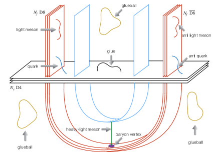
Figure 8: Strings as various hadrons in the D4/D8 model.

3.5 Theta dependence in QCD

In Yang-Mills theory, there could be an topological term proportional to the $\theta$ angle [112]. In the large $N_{c}$ limit, the full Lagrangian takes the form as,

$$S=\frac{N_{c}}{2\lambda}\mathrm{Tr}\int\ ^{\star}F\wedge F-i\frac{\lambda}{8\pi^{2}}\frac{\theta}{N_{c}}\mathrm{Tr}\int F\wedge F.$$ (3.88)

While the value of $\theta$ angle may be experimentally small, it leads to many interesting effects e.g. glueball spectrum [113], deconfinement transition [114, 115], chiral magnetic effect [116, 117], especially its large $N_{c}$ limit [118]. Since the D4/D8 model is a holographic version of QCD, it is possible to introduce the $\theta$ term to the dual theory through the gauge-gravity duality.

The main idea to include an Yang-Mills $\theta$ term in holography is to introduce coincident $N_{0}$ D0-branes acting to the $N_{c}$ D4-brane background (2.14). In this sense, we have to require $N_{0}/N_{c}$ is fixed when $N_{c}\rightarrow\infty$. And for the SUGRA approach, the dynamics of the Ramond-Ramond 1-form $C_{1}$ must be picked up into the IIA SUGRA action (2.15) in order to include the charge of the D0-branes as,

$$S_{\mathrm{IIA}}^{10\mathrm{d}}=\frac{1}{2\kappa_{10}^{2}}\int d^{10}x\sqrt{-G}e^{-2\phi}\left[\mathcal{R}^{(10)}+4\partial_{\mu}\phi\partial\phi\right]-\frac{1}{4\kappa_{10}^{2}}\int d^{10}x\sqrt{-G}\left(\left|F_{4}\right|^{2}+\left|F_{2}\right|^{2}\right),$$ (3.89)

where $F_{2}=dC_{1}$. To obtain an analytical solution, we assume the D0-branes are smeared homogeneous along $x^{4}$, hence the associated equations of motion to (3.89) can be solved as,

$$ds^{2} =H_{4}^{-1/2}\left[-H_{0}^{-1/2}f_{T}\left(U\right)\left(dx^{0}\right)^{2}+H_{0}^{1/2}dx_{i}dx^{i}\right]+H_{4}^{1/2}H_{0}^{1/2}\left[\frac{dU^{2}}{f_{T}\left(U\right)}+U^{2}d\Omega_{4}^{2}\right],$$

$$H_{4} =1+\frac{R^{3}}{U^{3}},H_{0}=1-\frac{U_{H}^{3}}{U^{3}}\frac{\Theta^{2}}{1+\Theta^{2}},e^{\phi}=H_{4}^{-1/4}H_{0}^{3/4},C_{1}=\frac{\Theta}{g_{s}}\frac{f_{T}}{H_{0}}dx^{4},F_{4}=3R^{3}g_{s}^{-1},$$ (3.90)

where $\Theta$ is a constant parameter. Take the near horizon limit so that $H_{4}\rightarrow R^{3}/U^{3}$ and impose the double Wick rotation as it is discussed in Section 2.1, we can obtain a D0-D4 bubble background associated to (2.16) as,

$$ds^{2} =H_{4}^{-1/2}\left[H_{0}^{1/2}\eta_{\mu\nu}dx^{\mu}dx^{\nu}+H_{0}^{-1/2}f\left(U\right)\left(dx^{4}\right)^{2}\right]+H_{4}^{1/2}H_{0}^{1/2}\left[\frac{dU^{2}}{f_{T}\left(U\right)}+U^{2}d\Omega_{4}^{2}\right],$$

$$H_{4} =\frac{R^{3}}{U^{3}},H_{0}=1-\frac{U_{KK}^{3}}{U^{3}}\frac{\Theta^{2}}{1+\Theta^{2}},e^{\phi}=H_{4}^{-1/4}H_{0}^{3/4},C_{1}=-i\frac{\Theta}{g_{s}}\frac{f}{H_{0}}dx^{4},F_{4}=3R^{3}g_{s}^{-1}.$$ (3.91)

Due to the presence of the D0-branes, we can see the dual theory to (3.91) is pure Yang-Mills theory with a $\theta$ term if a probe D4-brane located at the holographic boundary is taken into account as,

$$S_{\mathrm{D4}}= \big{[}-T_{\mathrm{D4}}\mathrm{STr}\int d^{4}xd\tau e^{-\phi}\sqrt{-\det\left(G+2\pi\alpha^{\prime}F\right)}+g_{s}T_{\mathrm{D4}}\int C_{5}$$

$$+\frac{1}{2}\left(2\pi\alpha^{\prime}\right)^{2}g_{s}T_{\mathrm{D4}}\int C_{1}\wedge F\wedge F\big{]}|_{U\rightarrow\infty}$$

$$\simeq -\frac{1}{2g_{\mathrm{YM}}^{2}}\mathrm{Tr}\int{}^{*}F\wedge F+i\frac{g_{\mathrm{YM}}^{2}}{8\pi^{2}}\theta\mathrm{Tr}\int F\wedge F+\mathcal{O}\left(F^{4}\right),$$ (3.92)

which further implies the bare $\theta$ angle relates to the $\Theta$ parameter in the solution (3.91) by

$$\Theta=\frac{\lambda}{8\pi^{2}}\left(\frac{\theta+2k\pi}{N_{c}}\right),k\in\mathbb{Z}$$ (3.93)

as a fixed constant in the large $N_{c}$ limit.

With the geometry background (3.91), it is possible to evaluate several properties of Yang-Mills theory with a $\theta$ term by following the discussions in previous sections and let us take a brief look at them for examples. First we focus on the the ground state energy which can be evaluated by using (3.1) - (3.5) as,

$$F\left(\Theta\right)=-\frac{2N_{c}^{2}\lambda}{3^{7}\pi^{2}}\frac{M_{KK}^{4}}{\left(1+\Theta^{2}\right)^{3}}.$$ (3.94)

In the expansion with respect to small $\Theta$, (3.94) reduces to minimized free energy difference,

$$\min_{k}\left[F\left(\Theta\right)-F\left(0\right)\right]\simeq\frac{1}{2}\chi_{g}\theta^{2}\left[1+\bar{b}_{2}\frac{\theta^{2}}{N_{c}^{2}}+\bar{b}_{4}\frac{\theta^{4}}{N_{c}^{4}}+\mathcal{O}\left(\theta^{6}\right)\right],$$ (3.95)

as the energy of the $\theta$ vacuum. And the topological susceptibility reads,

$$\chi_{g}=\frac{\lambda^{3}M_{KK}^{4}}{32\left(3\pi\right)^{6}},$$ (3.96)

with

$$\bar{b}_{2}=-\frac{\lambda^{2}}{32\pi^{4}},\bar{b}_{4}=-\frac{5\lambda^{4}}{3\times 2^{11}\pi^{8}}.$$ (3.97)

Moreover, one can consider a constant $C_{1}$ in the black D4-brane background (2.14) so that $F_{2}=dC_{1}=0$. Hence the ground state energy of deconfined Yang-Mills theory with a constant $\theta$ term can be identified to $F_{\mathrm{deconf}.}$ presented in (3.6). Then the QCD deconfinement phase transition can be obtained by comparing the free energy (3.94) with $F_{\mathrm{deconf}.}$ in (3.6) which leads to the critical temperature as,

$$T_{c}\left(\Theta\right)=\frac{M_{KK}}{2\pi}\frac{1}{\sqrt{1+\Theta^{2}}}\simeq\frac{M_{KK}}{2\pi}\left[1-\frac{\lambda^{2}}{128\pi^{4}}\frac{\theta^{2}}{N_{c}^{2}}+\frac{3\lambda^{4}}{2^{15}\pi^{8}}\frac{\theta^{4}}{N_{c}^{4}}+\mathcal{O}\left(\frac{\theta^{6}}{N_{c}^{6}}\right)\right].$$ (3.98)

Second, the QCD string tension also takes a correction due to the presence of $\theta$ term. Consider an open string stretched in the background (3.91) ending on a probe D4-brane at boundary. Use the AdS/CFT dictionary, the Wilson loop in the dual theory relates to the classical Nambu-Goto (NG) action $S_{NG}$ of the open string corresponding to the tension $T$ with quark potential $V$ as,

$$\left\langle W\left(\mathcal{C}\right)\right\rangle\sim e^{-S_{NG}}\sim e^{-TV}.$$ (3.99)

In the static gauge, the relevant string embedding can be chosen as

$$\tau=x^{0}\in\left[0,T\right],\sigma=x\in\left[-l/2,l/2\right],U=U\left(x\right),$$ (3.100)

then the NG action is given by

$$S_{NG}=-\frac{1}{2\pi\alpha^{\prime}}\int d\tau d\sigma\sqrt{-g_{\tau\tau}g_{\sigma\sigma}}=-\frac{1}{2\pi\alpha^{\prime}}\int d\tau d\sigma\sqrt{-g_{00}\left[g_{xx}+g_{UU}U^{\prime}\left(x\right)^{2}\right]},$$ (3.101)

To quickly evaluate the QCD tension, let us consider the limit $l\rightarrow\infty$. In this limit, the open string must minimize its energy as possible as it can, it forces the factor $\sqrt{-g_{00}g_{xx}}$ to become minimal to take the value at $U=U_{KK}$ since the size of $x^{4}$ shrinks at $U=U_{KK}$. Therefore the QCD tension $T_{s}$ is obtained from

$$S_{NG}\simeq-\frac{1}{2\pi\alpha^{\prime}}Tl\sqrt{-g_{00}g_{xx}}|_{U=U_{KK}}=-T_{s}Tl,$$ (3.102)

as

$$T_{s}=\frac{1}{2\pi\alpha^{\prime}}\sqrt{-g_{00}g_{xx}}|_{U=U_{KK}}=\frac{\lambda}{27\pi}M_{KK}^{2}\frac{1}{\left(1+\Theta^{2}\right)^{2}}.$$ (3.103)

Next, let us investigate the glueball mass with the background (3.91). As the glueball corresponds to the gravitational fluctuation, by adding a perturbation to metric presented in (3.91) as $g_{MN}\rightarrow g_{MN}+h_{MN}$, it reduces to equation of motion for $h_{MN}$ as

$$\frac{1}{2}\nabla_{M}\nabla_{N}h_{\ K}^{K}+\frac{1}{2}\nabla^{2}h_{MN}-\left(\nabla^{K}\nabla_{M}h_{NK}+\nabla^{K}\nabla_{N}h_{MK}\right)-\frac{3}{2}h_{MN}=0.$$ (3.104)

Here since IIA SUGRA can be obtained by the dimension reduction from 11d M-theory, $h_{MN}$ refers to the fluctuation on $\mathrm{AdS}_{7}$ which means $M,N$ runs over 0 - 6. Setting $h_{MN}=H_{MN}\left(U\right)e^{-ik\cdot x}$ with the ansatz

$$H_{MN}\left(U\right)=\frac{U}{R}H\left(U\right)\mathrm{diag}\left(0,1,1,1,0,-\frac{3}{1+\Theta^{2}},0\right),$$ (3.105)

it gives the eigen equation for $H\left(U\right)$ as,

$$H^{\prime\prime}\left(U\right)+\frac{4U^{3}-U_{KK}^{3}}{U\left(U^{3}-U_{KK}^{3}\right)}H^{\prime}\left(U\right)-\frac{M^{2}R^{2}}{U^{3}-U_{KK}^{3}}H\left(U\right)=0,$$ (3.106)

which implies the mass spectrum $M$ with a correction due to $\Theta$,

$$M\simeq\frac{M\left(0\right)}{\sqrt{1+\Theta^{2}}}.$$ (3.107)

The presence of $\theta$ also decreases the baryon mass $m_{B}$ as,

$$m_{B}=\frac{\lambda}{27\pi}N_{c}M_{KK}\frac{1}{\left(1+\Theta^{2}\right)^{3/2}},$$ (3.108)

by imposing the metric presented in (3.91) into (2.76) which implies the evidence of metastable particles in QCD. By further analyze the entanglement entropy on (3.91), it agree consistently with the property of the possible metastable states in this model. Besides, when we follow the discussion in Section 2.2, it is possible to introduce flavored meson in the D0-D4 background. And the meson mass also acquires the correction by the $\theta$ angle as [41, 42]. Further follow the instantonic description for baryon in Section 2.5, one can see the metastable baryonic spectrum in this model as [119]. In this sense, the Witten-Sakai-Sugimoto model in the D0-D4 brane background is recognized as a holographic version of QCD with a $\theta$ term.

4 Summary and outlook

In this review, we look back to the fundamental properties of the D4/D8 model which includes the D4-brane background, the embedding of the $\mathrm{D8/\overline{D8}}$-branes and how to identify meson, baryon, glueball in this model. Besides, we revisit some interesting topics about QCD by using this model which relates to the deconfinement transition, chiral phase, heavy flavor, various interaction of hadrons and the $\theta$ term in QCD. This review illustrates that string theory can provide a powerful method for studying the strongly coupled regime of QCD, which is out of reach for the traditional methods of perturbative QFT. We particularly note here there are additional interesting approaches based on this model absent in the main text of this review, they relates to the holographic Schwinger effect [120, 121, 122, 123], the fluid/gravity correspondence [124, 125, 126, 127, 128], corrections to the instanton as baryon [129, 130], the approaches to the D3/D7 model [131, 132] and applications to study neutron stars [133, 134]. With all of these achievements, it may be possible to work out an exactly holographic version of QCD based on the D4/D8 model in the future work, to reinterpret the fundamental element of strong interaction according to gauge-gravity duality.

5 Appendix A: The type II supergravity solution

In this appendix, let us collect the $\mathrm{D}_{p}$-brane solution in the type II SUGRA. We note that all the discussion in this appendix is valid to the gravity solution presented in the main text if we set $p=4$. In the string frame, the action for type II SUGRA sourced by a stack of $N_{p}$ coincident $\mathrm{D}_{p}$-branes can be written as,

$$S_{\mathrm{II}}=\frac{1}{2\kappa_{10}^{2}}\int d^{10}x\sqrt{-g}\left[e^{-2\phi}\left(\mathcal{R}+4\partial_{M}\phi\partial^{M}\phi\right)-\frac{g_{s}^{2}}{2}\left|F_{p+2}\right|^{2}\right],$$ (A-1)

where $2\kappa_{10}^{2}=16\pi G_{10}=\left(2\pi\right)^{7}l_{s}^{8}g_{s}^{2}$ is the 10d gravity coupling constant, $\mathcal{R},\phi,C_{p+1}$ is respectively the 10d curvature, dilaton and Ramond-Ramond $p+1$-form field with $F_{p+2}=dC_{p+1}$. Note that, in string theory the dilaton field may also be defined as $\Phi$ by

$$\Phi-\Phi_{0}=\phi,e^{\Phi_{0}}=g_{s}.$$ (A-2)

Since a $\mathrm{D}_{p}$-brane for $p=4,5,6$ is magnetically dual to $\mathrm{D}_{p}$-brane for $p=2,1,0$ and D3-brane is self dual, we only consider the case for $p<7$ in (A-1). Vary the action (A-1) with respect to $g_{MN},\phi,C_{p+1}$, the associated equations of motion are collected as,

$$0= \mathcal{R}+4\nabla^{2}\phi-4\left(\nabla\phi\right)^{2},$$

$$0= \partial_{N}\left(\sqrt{-g}F^{NM_{1}...M_{p+1}}\right),$$

$$0= \mathcal{R}_{MN}-\frac{1}{2}g_{MN}\mathcal{R}+2\nabla_{M}\nabla_{N}\phi+2g_{MN}\left(\nabla\phi\right)^{2}-2g_{MN}\nabla^{2}\phi$$

$$= \frac{g_{s}^{2}}{2\left(p+1\right)!}e^{2\phi}\left[F_{M}^{\ K_{1}...K_{p+1}}F_{NK_{1}...K_{p+1}}-\frac{\left(p+1\right)!}{2}g_{MN}\left|F_{p+2}\right|^{2}\right].$$ (A-3)

The solution for (A-3) can be obtained by using the simply homogeneous ansatz,

$$ds^{2} =H_{p}^{-\frac{1}{2}}\eta_{ab}dx^{a}dx^{b}+H_{p}^{\frac{1}{2}}\left(dr^{2}+r^{2}d\Omega_{8-p}^{2}\right),\ a,b=0,1...p$$

$$e^{\phi} =H_{p}^{-\frac{p-3}{4}},C_{01...p}=g_{s}^{-1}H_{p}^{-1},F_{r01...p}=\frac{\left(7-p\right)g_{s}^{-1}h_{p}^{7-p}}{r^{8-p}H_{p}^{2}},$$ (A-4)

where the harmonic function $H_{p}$ is solved through (A-3) as,

$$H_{p}\left(r\right)=1+\frac{h_{p}^{7-p}}{r^{7-p}}.$$ (A-5)

Here $r$ refers to the radial coordinate vertical to the $\mathrm{D}_{p}$-brane, $\Omega_{8-p}$ is the associated angle coordinate in the transverse space. The constant $h_{p}$ relates to the charge of the $\mathrm{D}_{p}$-brane computed as,

$$h_{p}^{7-p}=\left(2\sqrt{\pi}\right)^{5-p}g_{s}N_{p}\Gamma\left(\frac{7-p}{2}\right)l_{s}^{7-p}.$$ (A-6)

The solution (A-4) representing extremal black $\mathrm{D}_{p}$-branes reduces to the BPS condition as,

$$2\kappa_{10}^{2}g_{s}T_{\mathrm{D}_{p}}N_{p}=\int_{S^{8-p}}\ ^{\star}F_{p+2},$$ (A-7)

due to the action for the Ramond-Ramond (R-R) field $C_{p+1}$ with a source of $N_{p}$ coincident $\mathrm{D}_{p}$-branes,

$$S_{\mathrm{R-R}}=-\frac{1}{4\kappa_{10}^{2}}\int F_{p+2}\wedge\ ^{\star}F_{p+2}+g_{s}T_{\mathrm{D}_{p}}\int_{p+1}C_{p+1}.$$ (A-8)

The equations of motion (A-3) also allow the near-extremal solution as,

$$ds^{2} =H_{p}^{-\frac{1}{2}}\left[f\left(r\right)dt^{2}+\delta_{ij}dx^{i}dx^{j}\right]+H_{p}^{\frac{1}{2}}\left[\frac{dr^{2}}{f\left(r\right)}+r^{2}d\Omega_{8-p}^{2}\right],$$

$$e^{\phi} =H_{p}^{-\frac{p-3}{4}},C_{01...p}=g_{s}^{-1}H_{p}^{-1},F_{r01...p}=\frac{\left(7-p\right)g_{s}^{-1}h_{p}^{7-p}}{r^{8-p}H_{p}^{2}},$$ (A-9)

where $i,j$ run over the spacial index of the $\mathrm{D}_{p}$-branes. The functions $f\left(r\right),H_{p}\left(r\right)$ are solved respectively as,

$$f\left(r\right)=1-\frac{r_{H}^{7-p}}{r^{7-p}},H_{p}\left(r\right)=1+\frac{r_{p}^{7-p}}{r^{7-p}},$$ (A-9)

where $r_{H}$ refers to the horizon of the $\mathrm{D}_{p}$-branes. Notice the equation of motion (A-3) reduce to a constraint,

$$4\nabla_{M}\phi\nabla^{M}\phi-2\nabla^{2}\phi=\frac{p-3}{2}g_{s}^{2}e^{2\phi}\left|F_{p+2}\right|^{2},$$ (A-10)

which implies,

$$r_{p}^{7-p}=\sqrt{h_{p}^{2\left(7-p\right)}+\left(\frac{r_{H}^{7-p}}{2}\right)^{2}}-\frac{r_{H}^{7-p}}{2}.$$ (A-11)

So we have $r_{p}\rightarrow h_{p}$ if $r_{H}\rightarrow 0$, thus the near-extremal solution will return to the extremal solution in this limit.

6 Appendix B: Dimensional reduction for spinors

In this section, let us collect the dimensional reduction for spinor and one can see various boundary conditions determine the associated mass of fermion in lower dimension. Consider a complex massless spinor $\Psi$ in $\mathbb{R}^{d+1}$ satisfying Dirac equation,

$$\gamma^{M}\partial_{M}\Psi=0,$$ (B-1)

where $M$ runs over $\mathbb{R}^{d+1}$. When one of the spatial direction is compactified on a circle $S^{1}$, $\mathbb{R}^{d+1}$ becomes to $\mathbb{R}^{d}\times S^{1}$. Let us denote the coordinates on $\mathbb{R}^{d},S^{1}$ as $x^{\mu},y$ respectively. Then Fourier series of $\Psi$ can be written as the summary of its modes on $S^{1}$ as,

$$\Psi\left(x^{\mu},y\right)=\sum_{k}e^{\frac{iky}{L}}\psi_{k}\left(x^{\mu}\right),$$ (B-2)

where $L$ refers to the radius of $S^{1}$ and $k$ is integer or half integer. Thus the boundary of the spinor $\Psi$ can be periodic or anti-periodic as,

$$\Psi\left(x^{\mu},y\right)=\pm\Psi\left(x^{\mu},y+2\pi L\right),$$ (B-3)

for $k$ is integer and half integer respectively. Mostly, anti-periodic boundary condition for fermion is permitted since observables are usually the combination of even power of spinors. Inserting (B-2) into (B-1), it leads to,

$$\left(\gamma^{\mu}\partial_{\mu}-i\gamma_{*}\frac{k}{L}\right)\psi_{k}\left(x^{\mu}\right)=0,$$ (B-4)

where $\gamma_{*}=\gamma^{y}$. So we can see $\psi_{k}\left(x^{\mu}\right)$ is massive spinor in $\mathbb{R}^{d}$ with an effective mass $i\gamma_{*}\frac{k}{L}$ unless $k=0$. This implies under the dimension reduction, the spinor in lower dimension is always massive if the anti-periodic boundary condition is imposed. Note that in the low-energy theory, only the mode with minimal $k$ is the concern, thus it means fermion is massless/massive with periodic and anti-periodic boundary condition respectively in the low-energy theory.

7 Appendix C: Supersymmetric meson on the flavor brane

While the D4/D8 model achieves great success, it contains issues. The most important issue is that due to the remaining supersymmetry on the D8-branes, the D4/D8 model contains supersymmetrically fermionic meson (mesino) on the flavor $N_{f}$ $\mathrm{D8/\overline{D8}}$-branes which should not be presented in QCD [135]. As we have specified in Section 2.1 that the supersymmetry on $N_{c}$ D4-branes breaks down due to its compactified direction $x^{4}$, however there is not any mechanism to break down the supersymmetry on the flavor branes since the $N_{f}$ $\mathrm{D8/\overline{D8}}$-branes is perpendicular to the compactified direction $x^{4}$. Therefore in principle, there is no reason to neglect the supersymmetric fermions in this model. So let us pick up the fermionic action for the D8-branes additional to its bosonic action (2.22). Up to quadratic order, the fermionic action for the D8-brane reads [136, 137, 138],

$$S_{\mathrm{D8}}^{\left(f\right)}=i\frac{T_{\mathrm{D8}}}{2}\int d^{9}xe^{-\phi}\mathrm{STr}\sqrt{-\det\left[g_{ab}+\left(2\pi\alpha^{\prime}\right)\mathcal{F}_{ab}\right]}\bar{\Psi}\left(1-\Gamma_{\mathrm{D8}}\right)\left(\Gamma^{c}\hat{D}_{c}-\Delta+\hat{\mathrm{L}}_{D8}\right)\Psi,$$ (C-1)

where $\Psi$ refers to 32-component Majorana spinor in 10d spacetime and,

$$\Gamma_{\mathrm{D8}} =\frac{\sqrt{-\det\left[g_{ab}\right]}}{\sqrt{-\det\left[g_{ab}+\left(2\pi\alpha^{\prime}\right)\mathcal{F}_{ab}\right]}}\Gamma_{\mathrm{D8}}^{\left(0\right)}\Gamma^{11}\sum_{q}\frac{\left(-\Gamma^{11}\right)^{q}}{q!2^{q}}\Gamma^{a_{1}...a_{2q}}\mathcal{F}_{a_{1}a_{2}}...\mathcal{F}_{a_{2q-1}a_{2q}},$$

$$\hat{\mathrm{L}}_{D8} =-\frac{\sqrt{-\det\left[g_{ab}\right]}}{\sqrt{-\det\left[g_{ab}+\left(2\pi\alpha^{\prime}\right)\mathcal{F}_{ab}\right]}}\Gamma_{\mathrm{D8}}^{\left(0\right)}\sum_{q\geq 1}\frac{\left(-\Gamma^{11}\right)^{q-1}}{\left(q-1\right)!2^{q-1}}\Gamma^{a_{1}...a_{2q-1}}\mathcal{F}_{a_{1}a_{2}}...\mathcal{F}_{a_{2q-1}c}g^{bc}\hat{D}_{b},$$

$$\Gamma_{\mathrm{D8}}^{\left(0\right)} =\frac{\epsilon^{a_{1}...a_{9}}}{9!\sqrt{-\det\left[g_{ab}\right]}}\Gamma_{a_{1}...a_{9}}=-\Gamma^{11}\Gamma^{\underline{5}},$$

$$\Delta =\frac{1}{2}\Gamma^{M}\partial_{M}\phi-\frac{1}{8}\frac{1}{4!}g_{s}e^{\phi}F_{MNPQ}\Gamma^{MNPQ},$$

$$\hat{D}_{M} =\nabla_{M}-\frac{1}{8}\frac{1}{4!}g_{s}e^{\phi}F_{MNPQ}\Gamma^{MNPQ}\Gamma_{M},$$

$$\nabla_{M} =\partial_{M}+\frac{1}{4}\omega_{M}^{\ \ \underline{N}\underline{P}}\Gamma_{\underline{N}\underline{P}}.$$ (C-2)

The action (C-1) is the fermionic action for D8-brane obtained under T-duality. The notation in (C-1) and (C-2) is given as follows. The index labeled by capital letters $M,N,P,Q$ runs over 10d spacetime and labeled by lowercase letters runs over D8-brane. The index with underline corresponds to index in the flat tangent space used by elfbein e.g. $g_{MN}=e_{M}^{\underline{M}}\eta_{\underline{M}\underline{N}}e_{N}^{\underline{N}}$, so we have e.g. $\Gamma^{a}=g^{ab}\partial_{b}X^{M}e_{M}^{\underline{N}}\Gamma_{\underline{N}}$. $\Gamma^{M}$ refers to the Dirac matrix satisfying $\left\{\Gamma^{M},\Gamma^{N}\right\}=2g^{MN}$ and $\omega_{M}^{\ \ \underline{N}\underline{P}}$ refers to the spin connection. $F_{MNPQ}$ is the components of the Ramond-Ramond $F_{4}$ and $\phi$ is the dilaton field which are all given in Section 2. The gamma matrix $\Gamma^{MNPQ}$ is given by $\Gamma^{MNPQ}=\Gamma^{[M}\Gamma^{N}\Gamma^{P}\Gamma^{Q]}$. Here $\mathcal{F}_{ab}=F_{ab}+B_{ab}$ where $F_{ab}$ is the gauge field strength on the flavor brane and $B_{ab}$ is the antisymmetric tensor $B_{MN}$ induced on the flavor brane which can be set to zero.

Imposing the bubble solution given in (2.16) and supergravity solutions for the dilaton $\phi$ and Ramond-Ramond $F_{4}$ to(C-1), after some calculations it becomes,

$$S_{\mathrm{D8}}^{\left(f\right)}=\frac{iT}{\left(2\pi\alpha^{\prime}\right)^{2}\Omega_{4}}\int d^{4}xdZd\Omega_{4}\tilde{\Psi}P_{-}\left[\frac{2}{3}M_{KK}K^{-\frac{1}{2}}\Gamma^{\underline{m}}\nabla_{m}^{S^{4}}+K^{-2/3}\Gamma^{\underline{\mu}}\partial_{\mu}+M_{KK}\Gamma_{\underline{4}}\partial_{Z}\right]\Psi,$$ (C-3)

where $\Gamma^{\underline{m}}\nabla_{m}^{S^{4}}$ is the Dirac operator on $S^{4}$ i.e. the index $m$ runs over $S^{4}$ and,

$$\tilde{\Psi}=K^{-13/24}\Psi,K\left(Z\right)=1+Z^{2},T=\left(\frac{3}{2}\right)^{4}T_{\mathrm{D8}}\Omega_{4}\left(2\pi\alpha^{\prime}\right)^{2}\frac{\left(\frac{2}{3}M_{KK}R\right)^{21/2}}{M_{KK}^{5}},P_{-}=\frac{1}{2}\left(1-\Gamma_{\mathrm{D8}}\right).$$ (C-4)

Since we are interesting in the fermionic part, the gauge field included by $\mathcal{F}_{ab}$ has been turned off i.e. $\mathcal{F}_{ab}=0$. Afterwards, in order to obtain a 5d effective action as the mesonic action given in (2.33), we can decompose the spinor $\Psi$ into a 3+1 dimensional part $\psi\left(x,Z\right)$ as mesino, an $S^{4}$ part $\chi$ and a remaining 2d part $\lambda$ as,

$$\Psi=\psi\otimes\chi\left(S^{4}\right)\otimes\lambda.$$ (C-5)

And the associated gamma matrices can be chosen as,

$$\Gamma^{\underline{\mu}} =\sigma_{1}\otimes\gamma^{\underline{\mu}}\otimes\bm{1},\mu=0,1,2,3$$

$$\Gamma^{\underline{4}} =\sigma_{1}\otimes\gamma\otimes\bm{1},$$

$$\Gamma^{\underline{5}} =\sigma_{2}\otimes\bm{1}\otimes\tilde{\gamma},$$

$$\Gamma^{\underline{m}} =\sigma_{2}\otimes\bm{1}\otimes\tilde{\gamma}^{\underline{m}},m=6,7,8,9,$$

$$\gamma =i\gamma^{\underline{0}}\gamma^{\underline{1}}\gamma^{\underline{2}}\gamma^{\underline{3}},$$

$$\tilde{\gamma} =i\gamma^{\underline{6}}\gamma^{\underline{7}}\gamma^{\underline{8}}\gamma^{\underline{9}},$$ (C-6)

where $\sigma_{1,2,3}$ refer to the Pauli matrices. In this decomposition, the 10d chirality matrix takes a very simple form as $\Gamma^{11}=\sigma_{3}\otimes\bm{1}\otimes\bm{1}$. If we chose the $\sigma_{3}$ representation, $\lambda$ can be decomposed by the eigenstates of $\sigma_{3}$ with

$$\sigma_{3}\lambda_{\pm}=\lambda_{\pm},\sigma_{1}\lambda_{\pm}=\lambda_{\mp},\sigma_{2}\lambda_{\pm}=\pm i\lambda_{\mp},$$ (C-7)

where $\lambda_{\pm}$ refers to the two eigenstates of $\sigma_{3}$. Since the kappa symmetry fixes the condition $\Gamma^{11}\Psi=\Psi$, we have to chose $\lambda=\lambda_{+}$. Besides, as $\chi$ must satisfy the Dirac equation on $S^{4}$, it can be decomposed by the spherical harmonic function. So the eigenstates of $\Gamma^{\underline{m}}\nabla_{m}^{S^{4}}$ can be chosen as [139],

$$\Gamma^{\underline{m}}\nabla_{m}^{S^{4}}\chi^{\pm l,s}=i\Lambda_{l}^{\pm}\chi^{\pm l,s};\Lambda_{l}^{\pm}=\pm\left(2+l\right),l=0,1...$$ (C-8)

where $s,l$ are angular quantum numbers carried by spherical harmonic function.

Put (C-5) into (C-3) with the decomposition (C-6) - (C-8) for $\chi$ and $\lambda$, we finally reach to a 5d effective action for mesino field as,

$$S=iT\int d^{4}xdZ\bar{\psi}\left(-\frac{2}{3}M_{KK}\lambda K^{-1/2}+K^{-2/3}\gamma^{\underline{\mu}}\partial_{\mu}+M_{KK}\gamma\partial_{Z}\right)\psi.$$ (C-9)

The 5d mesino $\psi$ can be further decomposed by working with

$$\psi\left(x,Z\right)=\left(\begin{array}[]{c}\psi_{+}\\ \psi_{-}\end{array}\right)=\sum_{n}\left[\begin{array}[]{c}\psi_{+}^{\left(n\right)}\left(x\right)f_{+}^{\left(n\right)}\left(Z\right)\\ \psi_{-}^{\left(n\right)}\left(x\right)f_{-}^{\left(n\right)}\left(Z\right)\end{array}\right],$$ (C-10)

where $f_{\pm}^{\left(n\right)}\left(Z\right)$ are real eigenfunctions of the coupled equations

$$-\frac{2\lambda}{3}K^{-1/2}f_{+}^{\left(n\right)}+\partial_{Z}f_{+}^{\left(n\right)} =\Lambda_{n}M_{KK}K^{-2/3}f_{-}^{\left(n\right)},$$

$$-\frac{2\lambda}{3}K^{-1/2}f_{-}^{\left(n\right)}-\partial_{Z}f_{-}^{\left(n\right)} =\Lambda_{n}M_{KK}K^{-2/3}f_{+}^{\left(n\right)},$$ (C-11)

with the normalizations

$$T\int dZK^{-2/3}f_{i}^{\left(n\right)}f_{j}^{\left(m\right)}=\delta^{mn}\delta_{ij},\ i,j=+,-,$$ (C-12)

Plugging (C-10) - (C-12) into (C-9), the action takes the canonical form as ($M_{n}=\Lambda_{n}M_{KK}$)

$$S=-\int d^{4}x\sum_{n}\left\{\psi_{-}^{\left(n\right)\dagger}i\sigma^{\mu}\partial_{\mu}\psi_{-}^{\left(n\right)}+\psi_{+}^{\left(n\right)\dagger}i\bar{\sigma}^{\mu}\partial_{\mu}\psi_{+}^{\left(n\right)}+M_{n}\left[\psi_{-}^{\left(n\right)\dagger}\psi_{+}^{\left(n\right)}+\psi_{+}^{\left(n\right)\dagger}\psi_{-}^{\left(n\right)}\right]\right\}.$$ (C-13)

Defining the Dirac spinor written in the Wely basis as,

$$\psi^{\left(n\right)}=\left(\begin{array}[]{c}\psi_{+}^{\left(n\right)}\left(x\right)\\ \psi_{-}^{\left(n\right)}\left(x\right)\end{array}\right),$$ (C-14)

action (C-13) can be rewritten as, ($\left\{\gamma^{\mu},\gamma^{\nu}\right\}=2\eta^{\mu\nu}$)

$$S=i\int d^{4}x\sum_{n}\left[\bar{\psi}^{\left(n\right)}\gamma^{\mu}\partial_{\mu}\psi^{\left(n\right)}+M_{n}\bar{\psi}^{\left(n\right)}\psi^{\left(n\right)}\right],$$ (C-15)

leading to a standard action for fermion. As we can see, the fermionic action illustrates the mesino mass takes the same order of meson mass hence it should be not neglected in principle, and authors of [140] also confirm this conclusion which is consistent with the remaining supersymmetry on D8-branes.

Moreover, when the bosonic gauge field is turned on, action (C-1) reduces to interaction terms of meson and mesino up to $\mathcal{O}\left(\mathcal{F},\Psi^{2}\right)$ as,

$$S_{int}= i\frac{T_{\mathrm{D8}}}{4}\int d^{9}x\sqrt{-g}e^{-\phi}\bar{\Psi}\Gamma_{\underline{5}}\Gamma^{11}\Gamma^{ab}\mathcal{F}_{ab}\left(\Gamma^{c}\hat{D}_{c}-\Delta\right)\Psi$$

$$-i\frac{T_{\mathrm{D8}}}{2}\int d^{9}x\sqrt{-g}e^{-\phi}\bar{\Psi}\left(1-\Gamma_{\underline{5}}\right)\Gamma^{\underline{5}}\Gamma^{11}\Gamma^{a}\mathcal{F}_{a}^{\ b}\hat{D}_{b}\Psi.$$ (C-16)

Using the decomposition (2.46) for $A_{a}$ and (C-6) - (C-8) for $\Psi$, action (C-16) includes interaction of $\pi$ meson and mesino as

$$S_{int}= \frac{M_{KK}}{f_{\pi}M_{int}^{2}}\sum_{n,p}\int d^{4}x\partial_{\mu}\pi\big{[}M_{KK}t_{\pi,n,p}\bar{\psi}^{\left(n\right)}i\gamma^{\mu}\gamma^{n+p+1}\psi^{\left(p\right)}$$

$$+l_{\pi,n,p}\bar{\psi}^{\left(n\right)}\left(-\gamma\right)^{n+p+1}\partial^{\mu}\psi^{\left(p\right)},$$ (C-17)

where the coupling constant is evaluated numerically as,

$$t_{\pi,n,p} =\frac{1}{2}\int dZK^{-5/6}\left[f_{+}^{\left(n\right)}f_{+}^{\left(p\right)\prime}-f_{+}^{\left(p\right)}f_{+}^{\left(n\right)\prime}+iK^{-1/2}f_{+}^{\left(n\right)}f_{+}^{\left(p\right)}\right],$$

$$l_{\pi,n,p} =\int dZK^{-3/2}f_{+}^{\left(n\right)}f_{-}^{\left(p\right)}.$$ (C-18)

And one can further work out the interaction terms of $\rho$ meson and mesino similarly. Since there is not any mechanism to suppress the interaction of meson and mesino or break down the supersymmetry on the D8-brane, we have to take into account these interactions in this model in principle while they are absent in realistic QCD.

Although we do not attempt to figure out this issue completely in this review, we give some comments which may be suggestive. The way to break down the supersymmetry on D8-branes may follow the discussion in [23], that is to compactify one of the directions of D8-brane (which is vertical to the $N_{c}$ D4-branes) on another circle then impose the periodic and anti-periodic boundary condition to meson and mesino respectively. Afterwards the supersymmetry on D8-branes would break down then the spectrum of meson and mesino is separated by a energy scale $1/\beta_{s}$ where $\beta_{s}$ refers to the size of the compactified direction of D8-brane. Another alternative scheme is to consider that the bubble solution (2.16) has a period $\beta_{T}$ with $\beta_{T}\gg 1$, hence the dual theory is non-supersymmetric above the size $\beta_{T}$ if we perform the same dimension reduction as [23]. Therefore it means the supersymmetry gets to rise only at exactly zero temperature due to $\beta_{T}=1/T$ which is ideal case, out of reach physically. So the dual theory on the D8-brane would be non-supersymmetry at any finite temperature.

References

- [1] E. Witten, “Anti-de Sitter space and holography”, Adv.Theor.Math.Phys. 2 (1998) 253-291, arXiv:hep-th/9802150.
- [2] J. M. Maldacena, “The Large N limit of superconformal field theories and supergravity”, Adv.Theor.Math.Phys. 2 (1998) 231-252, arXiv: hep-th/9711200.
- [3] O. Aharony, S. S. Gubser, J. M. Maldacena, H. Ooguri and Y. Oz, “Large N field theories, string theory and gravity”, Phys. Rept. 323 (2000) 183, arXiv:hep-th/9905111.
- [4] J. Maldacena, “Wilson loops in large N field theories”, Phys.Rev.Lett. 80 (1998) 4859-4862, arXiv: hep-th/9803002.
- [5] S. Rey, S. Theisen, J. Yee, “Wilson-Polyakov loop at finite temperature in large N gauge theory and anti-de Sitter supergravity”, Nucl.Phys.B 527 (1998) 171-186, hep-th/9803135 .
- [6] A. Brandhuber, N. Itzhaki, J. Sonnenschein, S. Yankielowicz, “Wilson loops in the large N limit at finite temperature”, Phys.Lett.B 434 (1998) 36-40, arXiv: hep-th/9803137.
- [7] G. Policastro, D. T. Son, A. O. Starinets, “From AdS / CFT correspondence to hydrodynamics”, JHEP 09 (2002) 043, arXiv: hep-th/0205052.
- [8] D. T. Son, A.O. Starinets, “Minkowski space correlators in AdS / CFT correspondence: Recipe and applications”, JHEP 09 (2002) 042, arXiv: hep-th/0205051.
- [9] P. Kovtun, D. T. Son, A. O. Starinets, “Viscosity in strongly interacting quantum field theories from black hole physics”, Phys.Rev.Lett. 94 (2005) 111601, arXiv: hep-th/0405231.
- [10] N. Iqbal, H. Liu, “Real-time response in AdS/CFT with application to spinors”, Fortsch.Phys. 57 (2009) 367-384, arXiv: 0903.2596, arXiv: 0903.2596.
- [11] H. Liu, J. McGreevy, D. Vegh, “Non-Fermi liquids from holography”, Phys.Rev.D 83 (2011) 065029, arXiv: 0903.2477.
- [12] G. W. Semenoff, K. Zarembo, “Holographic Schwinger Effect”, Phys.Rev.Lett. 107 (2011) 171601, arXiv: 1109.2920.
- [13] S. Ryu, T.Takayanagi, “Holographic derivation of entanglement entropy from AdS/CFT ”, Phys.Rev.Lett. 96 (2006) 181602, arXiv: hep-th/0603001.
- [14] I. R. Klebanov, D.Kutasov, A.Murugan, “Entanglement as a probe of confinement”, Nucl.Phys.B 796 (2008) 274-293, arXiv: 0709.2140.
- [15] D. Harlow, “Jerusalem Lectures on Black Holes and Quantum Information”, Rev.Mod.Phys. 88 (2016) 015002, arXiv: 1409.1231.
- [16] D. J. Gross, F. Wilczek, “Ultraviolet Behavior of Nonabelian Gauge Theories”, Phys.Rev.Lett. 30 (1973) 1343-1346.
- [17] H. D. Politzer, “Reliable Perturbative Results for Strong Interactions?”, Phys.Rev.Lett. 30 (1973) 1346-1349.
- [18] J. Erlich, E. Katz, D. T. Son, M. A. Stephanov, “QCD and a holographic model of hadrons”, Phys.Rev.Lett. 95 (2005) 261602, arXiv: hep-ph/0501128.
- [19] A. Karch, E. Katz, D. T. Son, M. A. Stephanov, “Linear Confinement and AdS/QCD”, arXiv:hep-ph/0602229.
- [20] L. Rold, A. Pomarol, “Chiral symmetry breaking from five dimensional spaces”, Nucl.Phys.B 721 (2005) 79-97, arXiv: hep-ph/0501218.
- [21] J. Casalderrey-Solana, H. Liu, D. Mateos, K. Rajagopal, U. A. Wiedemann, “Gauge/Gravity Duality, Hot QCD and Heavy Ion Collisions”, Cambridge University Press 2011, arXiv: 1101.0618.
- [22] M. Kruczenski, D. Mateos, R. C. Myers, D. J. Winters, “Towards a holographic dual of large N(c) QCD”, JHEP 05 (2004) 041, arXiv: hep-th/0311270.
- [23] E. Witten, “Anti-de Sitter space, thermal phase transition, and confinement in gauge theories”, Adv. Theor. Math. Phys. 2 (1998), 505-532, arXiv:hep-th/9803131.
- [24] T. Sakai, S. Sugimoto, “Low energy hadron physics in holographic QCD”, Prog.Theor.Phys. 113 (2005) 843-882, arXiv:hep-th/0412141.
- [25] T. Sakai, S. Sugimoto, “More on a holographic dual of QCD”, Prog.Theor.Phys. 114 (2005) 1083-1118, arXiv: hep-th/0507073.
- [26] E. Witten, “Baryons and branes in anti-de Sitter space”, JHEP 07 (1998) 006, arXiv: hep-th/9805112.
- [27] H. Hata, T. Sakai, S. Sugimoto, S. Yamato, “Baryons from instantons in holographic QCD”, Prog.Theor.Phys. 117 (2007) 1157, arXiv:hep-th/0701280.
- [28] H. Hata, M. Murata, “Baryons and the Chern-Simons term in holographic QCD with three flavors”, Prog.Theor.Phys. 119 (2008) 461-490, arXiv:0710.2579.
- [29] N. R. Constable, R. C. Myers, “Spin-two glueballs, positive energy theorems and the AdS/CFT correspondence”, JHEP 9910 (1999) 037, arXiv:hep-th/9908175.
- [30] R. C. Brower, S. D. Mathur, C.-I. Tan, “Glueball spectrum for QCD from AdS supergravity duality”, Nucl.Phys. B587 (2000) 249–276, arXiv:hep-th/0003115.
- [31] K. Hashimoto, C. -I Tan, S. Terashima, “Glueball Decay in Holographic QCD”, Phys.Rev.D77:086001,2008, [arXiv:0709.2208].
- [32] F. Brünner, D. Parganlija, A. Rebhan, “Glueball Decay Rates in the Witten-Sakai-Sugimoto Model”, Phys.Rev. D91 (2015) no.10, 106002, (Erratum:) Phys.Rev. D93 (2016) no.10, 109903, arXiv:1501.07906.
- [33] O. Aharony, J. Sonnenschein, S. Yankielowicz, “A Holographic model of deconfinement and chiral symmetry restoration”, Annals Phys. 322 (2007) 1420-1443, arXiv: hep-th/0604161.
- [34] F. Bigazzi, A. L. Cotrone, “Holographic QCD with Dynamical Flavors”, JHEP 1501 (2015) 104, arXiv:1410.2443.
- [35] S. Li, T. Jia, “Dynamically flavored description of holographic QCD in the presence of a magnetic field”, Phys.Rev. D96 (2017) no.6, 066032, arXiv:1604.07197.
- [36] O. Bergman, G. Lifschytz, M. Lippert, “Holographic Nuclear Physics”, JHEP 11 (2007) 056, arXiv: 0708.0326.
- [37] S. Li, A. Schmitt, Q. Wang, “From holography towards real-world nuclear matter”, Phys.Rev.D 92 (2015) 2, 026006, arXiv: 1505.04886.
- [38] Y.Liu, I.Zahed, “Heavy–light mesons in chiral AdS/QCD”, Phys.Lett.B 769 (2017) 314-321, arXiv: 1611.04400.
- [39] Y.Liu, I.Zahed, “Holographic Heavy-Light Chiral Effective Action”, Phys.Rev.D 95 (2017) 5, 056022, arXiv: 1611.03757.
- [40] N.Kovensky, A.Schmitt, “Heavy Holographic QCD”, JHEP 02 (2020) 096, arXiv: 1911.08433.
- [41] C. Wu, Z. Xiao, D. Zhou, “Sakai-Sugimoto model in D0-D4 background”, Phys.Rev.D 88 (2013) 2, 026016, arXiv: 1304.2111.
- [42] S. Seki, S. Sin, “A New Model of Holographic QCD and Chiral Condensate in Dense Matter”, JHEP 10 (2013) 223, arXiv: 1304.7097.
- [43] L. Bartolini, F. Bigazzi, S. Bolognesi, A. L. Cotrone, A. Manenti, “Theta dependence in Holographic QCD”, JHEP 02 (2017) 029, arXiv: 1611.00048.
- [44] F. Bigazzi, A. L. Cotrone, R. Sisca, “Notes on Theta Dependence in Holographic Yang-Mills”, JHEP 08 (2015) 090, arXiv: 1506.03826.
- [45] F. Bigazzi, A. Caddeo, A. L. Cotrone, P. D. Vecchia, A. Marzolla, “The Holographic QCD Axion”, JHEP 12 (2019) 056, arXiv: 1906.12117.
- [46] K. Hashimoto, T. Sakai, S. Sugimoto, “Nuclear Force from String Theory”, Prog.Theor.Phys. 122 (2009) 427-476, arXiv: 0901.4449.
- [47] K. Hashimoto, N. Iizuka, P.Yi, “A Matrix Model for Baryons and Nuclear Forces”, JHEP 10 (2010) 003, arXiv: 1003.4988.
- [48] K. Hashimoto, N. Iizuka, “Three-Body Nuclear Forces from a Matrix Model”, JHEP 11 (2010) 058, arXiv: 1005.4412.
- [49] K. Hashimoto, Y. Matsuo, “Nuclear binding energy in holographic QCD”, Phys.Rev.D 104 (2021) 2, 026006, arXiv: 2103.03563.
- [50] S. Li, T. Jia, “Matrix model and Holographic Baryons in the D0-D4 background”, Phys.Rev.D 92 (2015) 4, 046007, arXiv: 1506.00068.
- [51] S. Li, T. Jia, “Three-body force for baryons from the D0-D4/D8 brane matrix model”, Phys.Rev.D 93 (2016) 6, 065051, arXiv: 1602.02259.
- [52] V. Kaplunovsky, J. Sonnenschein, “Searching for an Attractive Force in Holographic Nuclear Physics”, JHEP 05 (2011) 058, arXiv: 1003.2621.
- [53] K. Becker, M. Becker, J.H. Schwarz, “String theory and M-theory, A Modern Introduction”, Cambridge University Press 2007.
- [54] E. Witten, “String Theory Dynamics in Various Dimensions”, Nucl. Phys. B 443 (1995) 197, arXiv:hep-th/9503124.
- [55] S. Sugimoto, K. Takahashi, “QED and string theory”, JHEP 04 (2004) 051, arXiv: hep-th/0403247.
- [56] E. Antonyan, J.A. Harvey, S. Jensen, D. Kutasov, “NJL and QCD from String Theory”, arXiv:hep-th/0604017.
- [57] D. Z. Freedman, A. V. Proeyen, “Supergravity”, Cambridge University Press 2012.
- [58] G. Mandal, T. Morita, “Gregory-Laflamme as the confinement/deconfinement transition in holographic QCD”, JHEP 09 (2011) 073, arXiv: 1107.4048.
- [59] G. Mandal, T. Morita, “What is the gravity dual of the confinement/deconfinement transition in holographic QCD?”, J.Phys.Conf.Ser. 343 (2012) 012079, arXiv: 1111.5190.
- [60] C. V. Johnson, “D-branes”, Cambridge University Press 2006.
- [61] I. Zahed, G.E. Brown, “The Skyrme Model”, Phys.Rept. 142 (1986) 1-102.
- [62] E. Witten, “Global Aspects of Current Algebra”, Nucl. Phys. B 223 (1983), 422.
- [63] O. Kaymakcalan, S. Rajeev, J. Schechter, “Nonabelian Anomaly and Vector Meson Decays”, Phys. Rev. D 30 (1984), 594.
- [64] S. -J Rey, J. -T Yee, “Macroscopic strings as heavy quarks in large N gauge theory and anti-de Sitter supergravity”, Eur.Phys.J.C 22 (2001) 379-394, arXiv: hep-th/9803001.
- [65] D. J. Gross, H. Ooguri, “Aspects of large N gauge theory dynamics as seen by string theory”, Phys.Rev.D 58 (1998) 106002, arXiv: hep-th/9805129.
- [66] D. Tong, “TASI lectures on solitons: Instantons, monopoles, vortices and kinks”, TASI 2005, arXiv: hep-th/0509216.
- [67] E. Witten, “Current Algebra, Baryons, and Quark Confinement”, Nucl.Phys.B 223 (1983) 433-444.
- [68] Y. Seo, S. -J. Sin, “Baryon Mass in medium with Holographic QCD”, JHEP 04 (2008) 010, arXiv: 0802.0568.
- [69] G. Adkins, C. Nappi, E. Witten, “Static Properties of Nucleons in the Skyrme Model”, Nucl.Phys.B 228 (1983) 552.
- [70] P. Lau, S. Sugimoto, “Chern-Simons 5-form and Holographic Baryons”, Phys. Rev. D 95, 126007 (2017), arXiv:1612.09503.
- [71] D. Mateos, R. C. Myers, R. M. Thomson, “Thermodynamics of the brane”, JHEP 0705, 067 (2007), arXiv: hep-th/0701132.
- [72] A. B. -Bayona, “Holographic deconfinement transition in the presence of a magnetic field”, JHEP 1311, 168 (2013), arXiv:1307.6498.
- [73] F. Bigazzi, A. L. Cotrone, J. Mas, D. Mayerson, J. Tarrio, “D3-D7 Quark-Gluon Plasmas at Finite Baryon Density”, JHEP 1104, 060 (2011), arXiv:1101.3560.
- [74] A. L. Cotrone, J. Tarrio, “Consistent reduction of charged D3-D7 systems”, JHEP 1210, 164 (2012), arXiv:1207.6703.
- [75] F. Bigazzi, A. L. Cotrone, J. Tarrio, “Charged D3-D7 plasmas: novel solutions, extremality and stability issues”, JHEP 1307, 074 (2013), arXiv:1304.4802.
- [76] P. Benincasa, “A note on Holographic Renormalization of Probe D-Branes”, arXiv:0903.4356.
- [77] I. Papadimitriou, “Holographic renormalization as a canonical transformation”, JHEP 1011, 014 (2010), arXiv:1007.4592.
- [78] I. Papadimitriou, “Holographic Renormalization of general dilaton-axion gravity”, JHEP 1108, 119 (2011), arXiv:1106.4826.
- [79] D. Giataganas, N. Irges, “Flavor Corrections in the Static Potential in Holographic QCD”, Phys. Rev. D 85, 046001 (2012), arXiv:1104.1623.
- [80] A. Deuzeman, M. P. Lombardo, K. Miura, T. N. da Silva, E. Pallante, ‘”Phases of many flavors QCD : Lattice results”, PoS ConfinementX , 274 (2012), arXiv:1304.3245.
- [81] J. Braun, H. Gies, “Scaling laws near the conformal window of many-flavor QCD”, JHEP 1005, 060 (2010), arXiv:0912.4168.
- [82] J. Liao, E. Shuryak, “Effect of Light Fermions on the Confinement Transition in QCD-like Theories”, Phys. Rev. Lett. 109, 152001 (2012), arXiv:1206.3989.
- [83] G. S. Bali, F. Bruckmann, G. Endrodi, Z. Fodor, S. D. Katz, S. Krieg, A. Schafer, K. K. Szabo, “The QCD phase diagram for external magnetic fields”, JHEP 02 (2012) 044, arXiv: 1111.4956.
- [84] G. S. Bali, F. Bruckmann, G. Endrödi, S.D. Katz, A. Schäfer, “The QCD equation of state in background magnetic fields”, JHEP 08 (2014) 177, arXiv: 1406.0269.
- [85] K. Fukushima, Y. Hidaka, “Magnetic Catalysis Versus Magnetic Inhibition”, Phys.Rev.Lett. 110 (2013) 3, 031601, arXiv: 1209.1319.
- [86] E. S. Fraga, L. F. Palhares, “Deconfinement in the presence of a strong magnetic background: an exercise within the MIT bag model”, Phys.Rev.D 86 (2012) 016008, arXiv: 1201.5881.
- [87] S. Sachan, S. Siwach, “Thermodynamics of soft wall AdS/QCD at finite chemical potential”, Mod.Phys.Lett.A 27 (2012) 1250163, arXiv: 1109.5523.
- [88] S. Sachan, “Study of confinement/deconfinement transition in AdS/QCD with generalized warp factors”, Adv.High Energy Phys. 2014 (2014) 543526, arXiv: 1408.3230.
- [89] A. Sevrin, J. Troost, W. Troost, “The nonAbelian Born-Infeld action at order ”, Nucl.Phys.B 603 (2001) 389-412, arXiv: hep-th/0101192.
- [90] M. Rozali, H. -H. Shieh, M. V. Raamsdonk, J. Wu, “Cold Nuclear Matter In Holographic QCD”, JHEP 01 (2008) 053, arXiv: 0708.1322.
- [91] K. Ghoroku, K. Kubo, M. Tachibana, T. Taminato, F. Toyoda, “Holographic cold nuclear matter as dilute instanton gas”, Phys.Rev.D 87 (2013) 6, 066006, arXiv: 1211.2499.
- [92] B.-J. Schaefer, J. M. Pawlowski, J. Wambach, “The Phase Structure of the Polyakov–Quark-Meson Model”, Phys.Rev.D 76 (2007) 074023, arXiv: 0704.3234 .
- [93] B. -J. Schaefer, M. Wagner, J. Wambach, “Thermodynamics of (2+1)-flavor QCD: Confronting Models with Lattice Studies”, Phys.Rev.D 81 (2010) 074013, arXiv: 0910.5628.
- [94] Y. Nambu, G. J. -Lasinio, “Dynamical Model of Elementary Particles Based on an Analogy with Superconductivity. 1.”, Phys.Rev. 122 (1961) 345-358.
- [95] Y. Nambu, G. J. -Lasinio, “Dynamical model of elementary particles based on an analogy with superconductivity. II.”, Phys.Rev. 124 (1961) 246-254.
- [96] K. Fukushima, “Chiral effective model with the Polyakov loop”, Phys.Lett.B 591 (2004) 277-284, arXiv: hep-ph/0310121.
- [97] M. Buballa, “NJL model analysis of quark matter at large density”, Phys.Rept. 407 (2005) 205-376, arXiv: hep-ph/0402234.
- [98] S. B. Ruester, V. Werth, M. Buballa, I. A. Shovkovy, D. H. Rischke, “The Phase diagram of neutral quark matter: Self-consistent treatment of quark masses”, Phys.Rev.D 72 (2005) 034004, arXiv: hep-ph/0503184.
- [99] J. D. Walecka, “A Theory of highly condensed matter”, Annals Phys. 83 (1974) 491-529.
- [100] J. Boguta, A. R. Bodmer, “Relativistic Calculation of Nuclear Matter and the Nuclear Surface”, Nucl.Phys.A 292 (1977) 413-428.
- [101] S. Gallas, F. Giacosa, G. Pagliara, “Nuclear matter within a dilatation-invariant parity doublet model: the role of the tetraquark at nonzero density”, Nucl.Phys.A 872 (2011) 13-24, arXiv: 1105.5003.
- [102] S. Floerchinger, C. Wetterich, “Chemical freeze-out in heavy ion collisions at large baryon densities”, Nucl.Phys.A 890-891 (2012) 11-24, arXiv: 1202.1671.
- [103] R.C. Myers, “Dielectric-Branes”, JHEP 9912, 022 (1999), arXiv:hep-th/9910053.
- [104] Y. Liu, M. A. Nowak, “Hyperons and Θ s + in holographic QCD”, Phys.Rev.D 105 (2022) 11, 114021, arXiv: 2201.01791.
- [105] Y. Liu, I. Zahed, “Heavy Baryons and their Exotics from Instantons in Holographic QCD”, Phys.Rev.D 95 (2017) 11, 116012, arXiv: 1704.03412.
- [106] Y. Liu, I. Zahed, “Heavy and Strange Holographic Baryons”, Phys.Rev.D 96 (2017) 5, 056027, arXiv: 1705.01397.
- [107] S. Li, “The interaction of glueball and heavy-light flavoured meson in holographic QCD”, Eur.Phys.J.C 80 (2020) 9, 881, arXiv: 1809.10379.
- [108] BESIII Collaboration, “Measurement of yCP in oscillation using quantum correlations in at √s = 3.773GeV”, Phys. Lett. B 744(2015)339-346, arXiv:1501.01378.
- [109] CDF Collaboration, “Observation of Bs-Bsbar Oscillations”, Phys.Rev.Lett.97:242003,2006, arXiv:hep-ex/0609040.
- [110] Si-wen Li, “Glueball–baryon interactions in holographic QCD”, Phys.Lett. B773 (2017) 142-149, arXiv:1509.06914.
- [111] Si-wen Li, “Holographic description of heavy-flavored baryonic matter decay involving glueball”, Phys.Rev.D 99 (2019) 4, 046013, arXiv: 1812.03482.
- [112] E. Vicari, H. Panagopoulos, “Theta dependence of SU(N) gauge theories in the presence of a topological term”, Phys.Rept. 470 (2009) 93-150, arXiv: 0803.1593.
- [113] L. D. Debbio, G. M. Manca, H. Panagopoulos, A. Skouroupathis, E. Vicari, “Theta-dependence of the spectrum of SU(N) gauge theories”, JHEP 06 (2006) 005, arXiv: hep-th/0603041.
- [114] M. D’Elia, F. Negro, “Phase diagram of Yang-Mills theories in the presence of a ϑ term”, Phys.Rev.D 88 (2013) 3, 034503, arXiv: 1306.2919.
- [115] M. D’Elia, F. Negro, “ϑ dependence of the deconfinement temperature in Yang-Mills theories”, Phys.Rev.Lett. 109 (2012) 072001, arXiv: 1205.0538.
- [116] K. Fukushima, D. E. Kharzeev, H. J. Warringa, “The Chiral Magnetic Effect”, Phys.Rev.D 78 (2008) 074033, arXiv: 0808.3382.
- [117] D. E. Kharzeev, “The Chiral Magnetic Effect and Anomaly-Induced Transport”, Prog.Part.Nucl.Phys. 75 (2014) 133-151, arXiv: 1312.3348.
- [118] E. Witten, “Theta dependence in the large N limit of four-dimensional gauge theories”, Phys.Rev.Lett. 81 (1998) 2862-2865, arXiv: hep-th/9807109.
- [119] W. Cai, C. Wu, Z. Xiao, “Baryons in the Sakai-Sugimoto model in the D0-D4 background”, Phys.Rev.D 90 (2014) 10, 106001, arXiv: 1410.5549.
- [120] W. Cai, K. Li, S. Li, “Electromagnetic instability and Schwinger effect in the Witten–Sakai–Sugimoto model with D0–D4 background”, Eur.Phys.J.C 79 (2019) 11, 904, arXiv: 1612.07087.
- [121] K. Hashimoto, T. Oka, A. Sonoda, “Electromagnetic instability in holographic QCD”, JHEP 06 (2015) 001, arXiv: 1412.4254.
- [122] S. Li, S. Luo, H. Li, “Holographic Schwinger effect and electric instability with anisotropy”, JHEP 08 (2022) 206, arXiv: 2205.01885.
- [123] S. Li, “Holographic Schwinger effect in the confining background with D-instanton”, Eur.Phys.J.C 81 (2021) 9, 797, arXiv: 2005.11955.
- [124] C. Wu, Y. Chen, M. Huang, “Fluid/gravity correspondence: A nonconformal realization in compactified D4 branes”, Phys.Rev.D 93 (2016) 6, 066005, arXiv: 1508.04038.
- [125] C. Wu, Y. Chen, M. Huang, “Fluid/gravity correspondence: Second order transport coefficients in compactified D4-branes”, JHEP 01 (2017) 118, arXiv: 1604.07765.
- [126] C. Wu, Y. Chen, M. Huang, “Chiral vortical effect from the compactified D4-branes with smeared D0-brane charge”, JHEP 03 (2017) 082, arXiv: 1608.04922.
- [127] W. Cai, S. Li, “Sound waves in the compactified D0-D4 brane system”, Phys.Rev.D 94 (2016) 6, 066012, arXiv: 1608.04075.
- [128] P. Benincasa, A. Buchel, “Hydrodynamics of Sakai-Sugimoto model in the quenched approximation”, Phys.Lett.B 640 (2006) 108-115, arXiv: hep-th/0605076.
- [129] A. Imaanpur, “Correction to baryon spectrum in holographic QCD”, Phys.Lett.B 832 (2022) 137233, arXiv: 2206.13878.
- [130] S. Li, H. Li, S. Luo, “Corrections to the instanton configuration as baryon in holographic QCD”, Phys.Rev.D 106 (2022) 12, 126027, arXiv: 2209.12521.
- [131] S. Li, S. Luo, Y. Hu, “Holographic QCD3 and Chern-Simons theory from anisotropic supergravity”, JHEP 06 (2022) 040, arXiv: 2203.14489.
- [132] S. Li, S. Luo, M. Tan, “Three-dimensional Yang-Mills-Chern-Simons theory from a D3-brane background with D-instantons”, Phys.Rev.D 104 (2021) 6, 066008, arXiv: 2106.04038.
- [133] A. Schmitt, P. Shternin, “Reaction rates and transport in neutron stars”, Astrophys.Space Sci.Libr. 457 (2018) 455-574, arXiv: 1711.06520.
- [134] N. Kovensky, A. Poole, A. Schmitt, “Building a realistic neutron star from holography”, Phys.Rev.D 105 (2022) 3, 034022, arXiv: 2111.03374.
- [135] R. Heise, H. Svendsen, “A Note on fermions in holographic QCD”, JHEP 08 (2007) 065, arXiv: 0706.2253.
- [136] D. Marolf, L. Martucci, P. J. Silva, “Fermions, T-duality and effective actions for D-branes in bosonic backgrounds”, JHEP 04 (2003) 051, arXiv: hep-th/0303209.
- [137] D. Marolf, L. Martucci, P. J. Silva, “Actions and fermionic symmetries for D-branes in bosonic backgrounds”, JHEP 07 (2003) 019, arXiv: hep-th/0306066.
- [138] L. Martucci, J. Rosseel, D. Van den Bleeken, A. Van Proeyen, “Dirac actions for D-branes on backgrounds with fluxes”, Class. Quant. Grav. 22 (2005) 2745–2764, arXiv: hep-th/0504041.
- [139] R. Camporesi, A. Higuchi, “On the eigenfunctions of the Dirac operator on spheres and real hyperbolic spaces”, J. Geom. Phys. 20 (1996) 1–18, arXiv: gr-qc/9505009.
- [140] T. Nakas, K. S. Rigatos, “Fermions and baryons as open-string states from brane junctions”, JHEP 12 (2020) 157, arXiv: 2010.00025.