Exact Method of Moments for multi-dimensional population balance equations

Abstract

The unique properties of anisotropic and composite particles are increasingly being leveraged in modern particulate products. However, tailored synthesis of particles characterized by multi-dimensional dispersed properties remains in its infancy and few mathematical models for their synthesis exist. Here, we present a novel, accurate and highly efficient numerical approach to solve a multi-dimensional population balance equation, based on the idea of the exact method of moments for nucleation and growth [1]. The transformation of the multi-dimensional population balance equation into a set of one-dimensional integro-differential equations allows us to exploit accurate and extremely efficient numerical schemes that markedly outperform classical methods (such as finite volume type methods) which is outlined by convergence tests. Our approach not only provides information about complete particle size distribution over time, but also offers insights into particle structure. The presented scheme and its performance is exmplified based on coprecipitation of nanoparticles. For this process, a generic growth law is derived and parameter studies as well as convergence series are performed.

1 Introduction and problem definition

The modeling and efficient numerical approximations of multi-dimensional (MD) nanoparticle (NP) synthesis are increasingly required as the properties of anisotropic particles play a major role in various applications, including bio-nanosensors or catalysts [2, 3, 4]. In recent years, automated analysis of MD particle shape distributions – essential to validate and calibrate MD process models – has been demonstrated for a range of composite and anisotropic NPs [5, 6, 7], unlocking the possibility of using predictive modeling for MD-NP synthesis.

To this end, we here extend the recently derived exact Method of Moments (eMoM[1]) to MD population balance equations (PBEs). As an example, we study a class of balance laws describing coprecipitation of particles characterized by their size and composition, such as the seeded growth of nanoalloys. However, the scheme can be applied more generally and is also applicable to e.g., the modeling of shape anisotropic growth (see e.g., the kinetics analyzed in [8, 9]). In general, we study the following MD-PBE:

Definition 1.1 (Multi-dimensional population balance equation).

The evolution of the particle population $q$ can be macroscopically described by the following MD-PBE:

$$\begin{aligned} q_{t}(t,\boldsymbol{x})+\nabla_{\boldsymbol{x}}(\boldsymbol{\mathcal{G}}({\boldsymbol{c}}(t),\boldsymbol{x})q(t,\boldsymbol{x}))&=0,\\ q(0,\boldsymbol{x})&=q_{0}(\boldsymbol{x}),\end{aligned}$$ (1)

with $\boldsymbol{x}\in\mathcal{X}\subset\mathbb{R}^{n}$, $t\in[0,T]$. The concentration of the $i$-th educt species, i.e. ${\boldsymbol{c}}_{i}$, is defined by:

$${\boldsymbol{c}}_{i}(t) =\tfrac{1}{\mathcal{V}}\boldsymbol{m}_{i}(t)-\tfrac{\boldsymbol{\rho}_{i}}{\mathcal{V}}\iint\limits_{{\boldsymbol{\mathcal{X}}}}\boldsymbol{V}\!_{i}(\boldsymbol{x})q(t,\boldsymbol{x})\,\mathrm{d}\boldsymbol{x},$$ (2)

where $q$ denotes the particle number density, $t$ the process time, $\boldsymbol{x}$ the shape parametrization of the dispersed phase, $\boldsymbol{\mathcal{G}}$ the concentration-dependent growth rate in the first argument and shape in the second argument, $q_{0}$ the initial particle number density, ${\boldsymbol{c}}_{i}$ the concentration of the $i$-th educt species, $\boldsymbol{m}_{i}$ the total mass of the $i$-th precipitated component, $\mathcal{V}$ the reactor volume, $\boldsymbol{\rho}_{i}$ the density of the $i$-th species in the NPs, ${\boldsymbol{\mathcal{X}}}$ the set of admissible particle shapes, and $\boldsymbol{V}\!_{i}(\boldsymbol{x})$ the volume of the $i$-th component in a particle of shape $\boldsymbol{x}$.

Conservation of mass (eq. 2) for each component couples the PBE solution $q$ and the concentrations $c_{i}$, rendering the PBE eq. 1 and (2) a (multi-dimensional) nonlocal conservation law [10]. In this manuscript, we reformulate the MD-PBE purely in terms of the concentrations, i.e., the driving forces. This idea was recently applied to the one-dimensional case in [1]. The advantage of such a reformulation lies in reducing the MD-PBE eq. 1 to a set of one-dimensional integro-differential equations eq. 5. The resulting equations prescribing the time-evolution of the concentrations can then be efficiently discretized and numerically approximated. For the most simple case involving two-chemical components and the evolution of composite particles, this reformulation reduces the need for numerically approximating one three-dimensional function, here the number density function $q$, to approximating two one-dimensional functions, i.e., the evolution of the two concentrations $c_{i}$.

2 Multi-dimensional exact method of moments

Our aim is to derive a solely concentration-dependent (${\boldsymbol{c}}$) equation based on eq. 2. Using the method of characteristics, see e.g. [10], for a given concentration ${\boldsymbol{c}}$, the solution of eq. 1 can be stated as follows:

$$q(t,\boldsymbol{x}) =q_{0}(\boldsymbol{\xi^{\mathsf{c}}}[t,\boldsymbol{x}](0))\text{det}(D_{2}\boldsymbol{\xi^{\mathsf{c}}}[t,\boldsymbol{x}](0)),$$ (3)

with the characteristics satisfying:

$$\begin{aligned} \partial_{3}\boldsymbol{\xi^{\mathsf{c}}}[t,\boldsymbol{x}](\tau)&=\boldsymbol{\mathcal{G}}({\boldsymbol{c}}(\tau),\boldsymbol{\xi^{\mathsf{c}}}[t,\boldsymbol{x}](\tau)),\\ \boldsymbol{\xi^{\mathsf{c}}}[t,\boldsymbol{x}](t)&=\boldsymbol{x},\end{aligned}$$ (4)

for every $(\tau,t,\boldsymbol{x})\in[0,T]^{2}\times{\boldsymbol{\mathcal{X}}}$ for $T\in\mathbb{R}_{>0}$ and with ${\boldsymbol{\mathcal{X}}}\subset\mathbb{R}^{2}$. As the characteristics depend on the concentration, we have added the concentration ${\boldsymbol{c}}$ as a superscript to illustrate this dependency. By plugging the solution formula eq. 3 into eq. 2, and integrating by substitution using $\boldsymbol{x}=\boldsymbol{\xi^{\mathsf{c}}}[0,\boldsymbol{y}](t)$, we end up – assuming $\boldsymbol{V}\!_{i}(\boldsymbol{x})=0\,\forall\boldsymbol{x}\notin{\boldsymbol{\mathcal{X}}}$ – with the following integro-differential equation:

Definition 2.1 (Integral fixed-point-problem for the concentrations ${\boldsymbol{c}}$).

$${\boldsymbol{c}}_{i}(t) =\tfrac{1}{\mathcal{V}}\boldsymbol{m}_{i}(t)-\tfrac{\boldsymbol{\rho}_{i}}{\mathcal{V}}\iint_{{\boldsymbol{\mathcal{X}}}}\boldsymbol{V}\!_{i}(\boldsymbol{\xi^{\mathsf{c}}}[0,\boldsymbol{y}](t))q_{0}\left(\boldsymbol{y}\right)\,\mathrm{d}\boldsymbol{y}.$$ (5)

The idea of eMoM ([1]) is now to numerically approximate eq. 5 instead of eq. 1 and (2). With ${\boldsymbol{c}}$ as a solution of eq. 5, we can post hoc evaluate the PBE solution $q$ using eq. 3. Thus, to obtain the full PBE solution $q$, we only need to compute a small number (the number of components involved) of time-dependent scalar quantities, i.e., the concentration ${\boldsymbol{c}}$. Thus, the reformulation eq. 5 of eq. 1 and (2) is highly advantageous whenever eq. 4 can be solved analytically for an arbitrary but given concentration ${\boldsymbol{c}}$, which is indeed possible for a distinct class of growth law functions. In the following, we first introduce rather general growth kinetics for coprecipitation processes, and then derive the analytical solution of the corresponding characteristics equation.

3 Kinetics of coprecipitation

In this section, we derive – based on generic physical assumptions – the growth kinetics of NPs in a coprecipitation process, in which two educt species simultaneously assemble in one particle ensemble. This approach is, e.g., in line with the current process understanding of synthesized nanoalloys [11], but also applies to the synthesis of multi-component battery cathode materials such as nickel-manganese-cobalt hydroxide [12].

Figure 1: Sketch of the change in size ($\dot{r}$) and composition $(\dot{f})$ in the growth of alloy nanoparticles

We assume that the change in NP radius is given by the sum of two growth rates, which depend on the radius to the exponent $n$ and the two concentrations ${\boldsymbol{c}}_{1}$ and ${\boldsymbol{c}}_{2}$, i.e.:

$$\dot{r}(t)=\left(\boldsymbol{G}_{1}({\boldsymbol{c}}_{1}(t))+\boldsymbol{G}_{2}({\boldsymbol{c}}_{2}(t))\right)r(t)^{n},$$ (6)

where $\boldsymbol{G}_{1}$ and $\boldsymbol{G}_{2}$ denote the growth kinetics of the two species. For the change in NP size, we can thus model, e.g. size-independent growth, i.e. $n=0$ [13], or diffusion-limited growth, i.e., $n=-1$ [14, 15].
For a particle with a given radius ($r>0$), we further define the volume fraction or composition $f$ and its derivative as:

$$\begin{aligned} f(t)&=\tfrac{\boldsymbol{v}_{1}(t)}{\boldsymbol{v}_{1}(t)+\boldsymbol{v}_{2}(t)},\\ \dot{f}(t)&=\tfrac{\dot{\boldsymbol{v}_{1}}(t)}{\boldsymbol{v}_{1}(t)+\boldsymbol{v}_{2}(t)}-f(t)\tfrac{\dot{\boldsymbol{v}_{1}}(t)+\dot{\boldsymbol{v}_{2}}(t)}{\boldsymbol{v}_{1}(t)+\boldsymbol{v}_{2}(t)}.\end{aligned}$$ (7)

Here, $\boldsymbol{v}_{1}(t)$ and $\boldsymbol{v}_{2}(t)$ are the volumes of the first and second chemical components in the NP at time $t$, respectively. Clearly, $\boldsymbol{v}_{1}(t)+\boldsymbol{v}_{2}(t)=\frac{4}{3}\pi r(t)^{3}$, and thus $\dot{\boldsymbol{v}}_{1}(t)+\dot{\boldsymbol{v}}_{2}(t)=4\pi r^{2}\dot{r}=4\pi r^{n+2}\left(\boldsymbol{G}_{1}({\boldsymbol{c}}_{1}(t))+\boldsymbol{G}_{2}({\boldsymbol{c}}_{2}(t))\right)$. As $\boldsymbol{v}_{1}(t)$ and $\boldsymbol{v}_{2}(t)$ can only change due to $\boldsymbol{G}_{1}({\boldsymbol{c}}_{1}(t))$ and $\boldsymbol{G}_{2}({\boldsymbol{c}}_{2}(t))$, respectively, we can assign $\dot{\boldsymbol{v}}_{1}(t)=4\pi r^{n+2}\boldsymbol{G}_{1}({\boldsymbol{c}}_{1}(t))$, and $\dot{\boldsymbol{v}}_{2}(t)=4\pi r^{n+2}\boldsymbol{G}_{2}({\boldsymbol{c}}_{2}(t))$. Now substituting the volume derivatives into eq. 7 with the identity $\boldsymbol{v}_{1}(t)+\boldsymbol{v}_{2}(t)=\frac{4}{3}\pi r(t)^{3}$, we obtain the following growth kinetics describing the change in radius and volume composition for given a radius, composition, and concentrations:

$$\boldsymbol{\mathcal{G}}({\boldsymbol{c}}(t),\boldsymbol{x}) =\begin{pmatrix}\tfrac{\boldsymbol{G}_{1}({\boldsymbol{c}}_{1}(t))+\boldsymbol{G}_{2}({\boldsymbol{c}}_{2}(t))}{\boldsymbol{x}_{1}^{-n}}\\ \tfrac{3\boldsymbol{G}_{1}({\boldsymbol{c}}_{1}(t))-3\left(\boldsymbol{G}_{1}({\boldsymbol{c}}_{1}(t))+\boldsymbol{G}_{2}({\boldsymbol{c}}_{2}(t))\right)\boldsymbol{x}_{2}}{\boldsymbol{x}_{1}^{1-n}}\end{pmatrix}.$$ (8)

Note that $\boldsymbol{x}_{1}$ and $\boldsymbol{x}_{2}$ denote the radius and the volume fraction coordinates, respectively. The characteristics ODE eq. 4 with the growth kinetics eq. 8 can be solved analytically for given time-dependent concentrations ${\boldsymbol{c}}$:

$$\boldsymbol{\xi^{\mathsf{c}}}_{\!\!\!1}[t,\boldsymbol{x}](\tau)$$

$$=\bigg{(}\!\boldsymbol{x}_{1}^{1-n}+(1-n)\!\int_{t}^{\tau}\!\!\!\!\boldsymbol{G}_{1}({\boldsymbol{c}}_{1}(s))+\boldsymbol{G}_{2}({\boldsymbol{c}}_{2}(s))\,\mathrm{d}s\bigg{)}^{\!\!\frac{1}{1-n}},$$ (9)

$$\boldsymbol{\xi^{\mathsf{c}}}_{\!\!\!2}[t,\boldsymbol{x}](\tau)$$

$$=3\int_{t}^{\tau}\tfrac{\boldsymbol{G}_{1}({\boldsymbol{c}}_{1}(\omega))}{\boldsymbol{\xi^{\mathsf{c}}}_{\!\!\!1}[t,\boldsymbol{x}](\omega)^{1-n}}e^{-3\int^{\tau}_{\omega}\frac{\left(\boldsymbol{G}_{1}({\boldsymbol{c}}_{1}(\eta))+\boldsymbol{G}_{2}({\boldsymbol{c}}_{2}(\eta))\right)}{\boldsymbol{\xi^{\mathsf{c}}}_{\!\!\!1}[t,\boldsymbol{x}](\eta)^{1-n}}d\eta}d\omega$$

$$\qquad+\boldsymbol{x}_{2}e^{-3\int_{t}^{\tau}\frac{\left(\boldsymbol{G}_{1}({\boldsymbol{c}}_{1}(\eta))+\boldsymbol{G}_{2}({\boldsymbol{c}}_{2}(\eta))\right)}{\boldsymbol{\xi^{\mathsf{c}}}_{\!\!\!1}[t,\boldsymbol{x}](\eta)^{1-n}}d\eta},$$ (10)

for $t,\tau\in[0,T]$, and $\boldsymbol{x}\in{\boldsymbol{\mathcal{X}}}:=\mathbb{R}_{\geq\boldsymbol{x}_{n}}\times[0,1]$ with minimal particle radius $\boldsymbol{x}_{n}\in\mathbb{R}_{>0}$. The fixed-point problem eq. 5 with the analytical solution of the characteristics eq. 9 and (10) will be discretized in the following section.

4 Numerical approximation of the fixed point problem

We can discretize the integro-differential equation by decomposing the time domain: $0=\boldsymbol{t}_{1}<\boldsymbol{t}_{2}<\cdots<\boldsymbol{t}_{N_{t}}=T$ into ${N_{t}}+1$ time steps, and quadrature points $(\boldsymbol{x}_{\ell})_{\ell=1\ldots,N_{t}}\subset\mathcal{X}^{N}_{t}$, with quadrature weights $(\boldsymbol{\omega}_{\ell})_{\ell=1\ldots,N_{t}}\subset\mathbb{R}^{N_{t}}_{>0}$, such that:

$$\iint_{\mathcal{X}}q_{0}(x)V(x)\,\mathrm{d}x\approx\sum_{\ell=1}^{N_{t}}q_{0}(\boldsymbol{x}_{\ell})\boldsymbol{\omega}_{\ell}.$$ (11)

Taking advantage of the semi-group property of the characteristics, i.e., $\boldsymbol{\xi^{\mathsf{c}}}[s,\boldsymbol{\xi^{\mathsf{c}}}[t,\boldsymbol{x}](s)](\tau)=\boldsymbol{\xi^{\mathsf{c}}}[t,\boldsymbol{x}](\tau)$ (see e.g. [16]) which also holds for its discretized version $\boldsymbol{\hat{\xi}^{\mathsf{C}}}$, we can approach this very efficiently as described in Algorithm 1 using the abbreviations ${\boldsymbol{\tilde{\xi}^{\mathsf{c}}}}(\ell,k):={\boldsymbol{\hat{\xi}^{\mathsf{C}}}}(1,\boldsymbol{x}_{\ell},k)\approx\boldsymbol{\xi^{\mathsf{c}}}(\boldsymbol{t}_{1},\boldsymbol{x}_{\ell},\boldsymbol{t}_{k})$ and ${\boldsymbol{\delta}}_{k}:=\boldsymbol{t}_{k+1}-\boldsymbol{t}_{k}$. In Algorithm 1, the computed $\boldsymbol{\mathsf{C}}_{i,k}$ is an approximation of the concentration of the $i$-th component at time $t_{k}$, i.e. $\boldsymbol{\mathsf{C}}_{i,k}\approx{\boldsymbol{c}}_{i}(\boldsymbol{t}_{k})$.

 

[5pt] initialization step

[20pt]

for $\ell=1\ldots Nx$ do

       $\boldsymbol{\tilde{\xi}^{\mathsf{c}}}(\ell,1)\leftarrow\boldsymbol{x}_{\ell}$

end for

$\boldsymbol{\mathsf{C}}_{1,1}\leftarrow\tfrac{1}{\mathcal{V}}\boldsymbol{m}_{1}(\boldsymbol{t}_{1})-\tfrac{\boldsymbol{\rho}_{1}}{\mathcal{V}}\sum_{\ell=1}^{N_{x}}\boldsymbol{V}\!_{1}\left(\boldsymbol{x}_{\ell}\right)q_{0}(\boldsymbol{x}_{\ell})\boldsymbol{\omega}_{\ell}$

$\boldsymbol{\mathsf{C}}_{2,1}\leftarrow\tfrac{1}{\mathcal{V}}\boldsymbol{m}_{2}(\boldsymbol{t}_{1})-\tfrac{\boldsymbol{\rho}_{2}}{\mathcal{V}}\sum_{\ell=1}^{N_{x}}\boldsymbol{V}\!_{2}\left(\boldsymbol{x}_{\ell}\right)q_{0}(\boldsymbol{x}_{\ell})\boldsymbol{\omega}_{\ell}$

[20pt]

time-stepping

[10pt]

for $k=1\ldots N_{t}-1$ do

       for $\ell=1\ldots Nx$ do

             $\boldsymbol{\tilde{\xi}^{\mathsf{c}}}(\ell,k+1)\leftarrow\begin{pmatrix}\left(\boldsymbol{\tilde{\xi}^{\mathsf{c}}}_{\negthickspace\negthickspace 1}(\ell,k)^{1-n}+(1-n){\boldsymbol{\delta}}_{k}\left(\boldsymbol{G}_{1}(\boldsymbol{\mathsf{C}}_{1,k})+\boldsymbol{G}_{2}(\boldsymbol{\mathsf{C}}_{2,k})\right)\right)^{\frac{1}{1-n}}\\ \left(3\tfrac{\boldsymbol{G}_{1}(\boldsymbol{\mathsf{C}}_{1,k}){\boldsymbol{\delta}}_{k}}{\boldsymbol{\tilde{\xi}^{\mathsf{c}}}_{\negthickspace\negthickspace 1}(\ell,k)^{1-n}}+\boldsymbol{\tilde{\xi}^{\mathsf{c}}}_{\negthickspace\negthickspace 2}(\ell,k)\right)\exp\left(-3\tfrac{\left(\boldsymbol{G}_{1}(\boldsymbol{\mathsf{C}}_{1,k})+\boldsymbol{G}_{2}(\boldsymbol{\mathsf{C}}_{2,k})\right){\boldsymbol{\delta}}_{k}}{\boldsymbol{\tilde{\xi}^{\mathsf{c}}}_{\negthickspace\negthickspace 1}(\ell,k)^{1-n}}\right)\end{pmatrix}$

       end for

      $\boldsymbol{\mathsf{C}}_{1,k+1}\leftarrow\tfrac{1}{\mathcal{V}}\boldsymbol{m}_{1}(\boldsymbol{t}_{k+1})-\tfrac{\boldsymbol{\rho}_{1}}{\mathcal{V}}\sum_{\ell=1}^{N_{x}}\boldsymbol{V}\!_{1}\left(\boldsymbol{\tilde{\xi}^{\mathsf{c}}}(\ell,k+1)\right)q_{0}(\boldsymbol{x}_{\ell})\boldsymbol{\omega}_{\ell}$

      $\boldsymbol{\mathsf{C}}_{2,k+1}\leftarrow\tfrac{1}{\mathcal{V}}\boldsymbol{m}_{2}(\boldsymbol{t}_{k+1})-\tfrac{\boldsymbol{\rho}_{2}}{\mathcal{V}}\sum_{\ell=1}^{N_{x}}\boldsymbol{V}\!_{2}\left(\boldsymbol{\tilde{\xi}^{\mathsf{c}}}(\ell,k+1)\right)q_{0}(\boldsymbol{x}_{\ell})\boldsymbol{\omega}_{\ell}$

end for

Algorithm 1 Numerical approximation scheme for the integral-fixed-point equation eq. 5 which prescribes the evolution of the driving forces over process time.

As the complexity of every iteration step is of order $N_{x}$ and we have $N_{t}$ steps, this approach yields the order $\mathcal{O}(N_{x}N_{t})$ in the numerical scheme.

To study the numerical performance of MD-eMoM, we conduct a numerical error analysis by refinement series. We assume the following growth kinetics: $\boldsymbol{G}_{1}(c)=c$, $\mathcal{V}=1$, ${\boldsymbol{c}}_{1}(0)={\boldsymbol{c}}_{2}(0)=2$, $\boldsymbol{\rho}_{1}=\boldsymbol{\rho}_{2}=1$, $\boldsymbol{V}\!_{1}(\boldsymbol{x})=\frac{4}{3}\pi\boldsymbol{x}_{1}^{3}\boldsymbol{x}_{2}$, and $\boldsymbol{V}\!_{2}(\boldsymbol{x})=\frac{4}{3}\pi\boldsymbol{x}_{1}^{3}(1-\boldsymbol{x}_{2})$; and take as initial datum $q_{0}(\boldsymbol{x})=\max\big{\{}1-(\boldsymbol{x}_{1}-\bar{\boldsymbol{x}}_{1})^{2}\delta_{1}^{-2}+(\boldsymbol{x}_{2}-\bar{\boldsymbol{x}}_{2})^{2}{\boldsymbol{\delta}}_{2}^{-2}\ ,0\big{\}}^{2}$, with $\bar{\boldsymbol{x}}=(0.1,0.75)^{\top}$ and ${\boldsymbol{\delta}}=(0.05,0.25)^{\top}$. To emphasize the impact of different growth kinetics on the composition evolution, we consider different growth rates for the second educt component ($\boldsymbol{G}_{2}$). The effect of different growth rate ratios $\boldsymbol{G}_{2}/\boldsymbol{G}_{1}$ on the temporal concentration evolution of each component is shown in Figure 2 (leftmost figure). The numerical approximation error w.r.t. changes in the discretization is shown in the middle (on the basis of the degrees of freedom $N_{x}N_{t}$) and right plot (on the basis of the computational time). The computational time refers to a vectorized MATLAB R2021b implementation of Algorithm 1 on a MacBook Pro 2021, Apple M1 Chip with 32GB RAM. In the same manner, higher-order explicit or implicit discretization schemes can easily be derived.

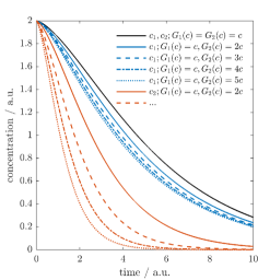
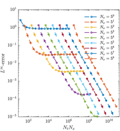
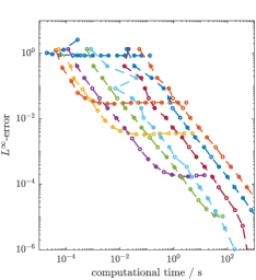
Figure 2: Solute concentrations over process time for different growth kinetics (left); Numerical approximation of the maximal absolute error in the concentrations ($L^{\infty}$-error) for different time discretizations $N_{t}$, and disperse property discretizations of the disperse property as a function of the number of degrees of freedom (DoF) $N_{t}N_{x}$ (middle); and the total computational time (right). The error analysis is performed for $\boldsymbol{G}_{1}(c)=c,\boldsymbol{G}_{2}(c)=5c$. The reference solution is given by $N_{t}\approx 10^{6},\&\ N_{x}\approx 4\;10^{5}$. For fixed $N_{x}$, we obtain a clear first-order behavior with respect to both the DoF and to the computational time, provided the spatial resolution is large enough.

5 Numerical approximation of the population balance equation solution

The PBE solution can be accessed in two different ways based on the solution of the fixed-point equation. Firstly, the particle density function for a given disperse property $\boldsymbol{x}\in{\boldsymbol{\mathcal{X}}}$ at a given time $t$, i.e., $q(t,\boldsymbol{x})$, is already given by eq. 3. Secondly, the solution can be evaluated with the introduced characteristics $\boldsymbol{\xi^{\mathsf{c}}}$, i.e.:

$$q(t,\boldsymbol{\xi^{\mathsf{c}}}[0,\boldsymbol{x}](t))=q_{0}(\boldsymbol{x})\ \text{det}\left(D_{2}\boldsymbol{\xi^{\mathsf{c}}}[t,\boldsymbol{\xi^{\mathsf{c}}}[0,\boldsymbol{x}](t)](0)\right).$$ (12)

To evaluate both solution formulas, we approximate the characteristics stated in eq. 9 and (10) by discretizing the integrals into the time interval and then approximating the integrands by the interval’s value at the lower time bound, i.e.:

$$\begin{split}&\boldsymbol{\xi^{\mathsf{c}}}_{\!\!\!1}[\boldsymbol{t}_{k},\boldsymbol{x}](\boldsymbol{t}_{i})\\ &\quad\approx\Big{(}\boldsymbol{x}_{1}^{1-n}+(1-n)\textstyle\sum_{\ell=k}^{i-1}\textbf{G}_{\ell}\Big{)}^{\frac{1}{1-n}}\\ &\quad=:\boldsymbol{\hat{\xi}^{\mathsf{C}}}_{\!\!\!\!\!1}\,(k,\boldsymbol{x},i),\\[10.0pt] &\boldsymbol{\xi^{\mathsf{c}}}_{\!\!\!2}[\boldsymbol{t}_{k},\boldsymbol{x}](\boldsymbol{t}_{i})\\ &\quad\approx 3\sum_{\ell=k}^{i-1}\frac{\boldsymbol{G}_{1}(\boldsymbol{\mathsf{C}}_{1,\ell})(\boldsymbol{t}_{\ell+1}-\boldsymbol{t}_{\ell})e^{-3\sum_{j=\ell}^{i-1}\frac{\textbf{G}_{j}}{\boldsymbol{\hat{\xi}^{\mathsf{C}}}_{\!\!\!\!\!1}\,(k,\boldsymbol{x},j)^{1-n}}}}{\boldsymbol{\hat{\xi}^{\mathsf{C}}}_{\!\!\!\!\!1}\,\!(k,\boldsymbol{x},\ell)^{1-n}}\\ &\qquad\qquad+\boldsymbol{x}_{2}e^{-3\sum_{\ell=k}^{i-1}\frac{\textbf{G}_{\ell}}{\boldsymbol{\hat{\xi}^{\mathsf{C}}}_{\!\!\!\!\!1}\,(k,\boldsymbol{x},\ell)^{1-n}}}\\ &\quad=:\boldsymbol{\hat{\xi}^{\mathsf{C}}}_{\!\!\!\!\!2}\,(k,\boldsymbol{x},i),\end{split}$$ (13)

with

$$\textbf{G}_{\ell}:=\big{(}\boldsymbol{G}_{1}(\boldsymbol{\mathsf{C}}_{1,\ell})+\boldsymbol{G}_{2}(\boldsymbol{\mathsf{C}}_{2,\ell})\big{)}\big{(}\boldsymbol{t}_{\ell+1}-{\boldsymbol{t}_{\ell}}\big{)}$$

The above equation holds for $k\leq i$. If $k>i$, the summations have to be understood as follows: $\sum_{\ell=k}^{i-1}=-\sum_{\ell=i}^{k-1}$. The solution of the PBE can then be approximated as follows:

$$\begin{split}q(\boldsymbol{t}_{k},\boldsymbol{x})\approx q_{0}\left(\boldsymbol{\hat{\xi}^{\mathsf{C}}}(k,\boldsymbol{x},1)\right)\left(\frac{\boldsymbol{\hat{\xi}^{\mathsf{C}}}_{\!\!\!\!\!1}\,(k,\boldsymbol{x},1)}{\boldsymbol{x}_{1}}\right)^{n}\Psi_{k,k}(x),\\ q\left(\boldsymbol{t}_{k},\boldsymbol{\hat{\xi}^{\mathsf{C}}}(1,\boldsymbol{x},k)\right)\approx q_{0}(\boldsymbol{x})\left(\frac{\boldsymbol{x}_{1}}{\boldsymbol{\hat{\xi}^{\mathsf{C}}}_{\!\!\!\!\!1}\,(1,\boldsymbol{x},k)}\right)^{n}\Psi_{1,k}(x).\end{split}$$ (14)

with

$$\Psi_{i,k}(x):=\exp\left(3\sum_{\ell=1}^{k-1}\frac{\left(\boldsymbol{G}_{1}(\boldsymbol{\mathsf{C}}_{1,\ell})+\boldsymbol{G}_{2}(\boldsymbol{\mathsf{C}}_{2,\ell})\right)\left(\boldsymbol{t}_{\ell+1}-\boldsymbol{t}_{\ell}\right)}{\boldsymbol{\hat{\xi}^{\mathsf{C}}}_{\!\!\!\!\!1}\,(i,\boldsymbol{x},\ell)^{1-n}}\right)$$

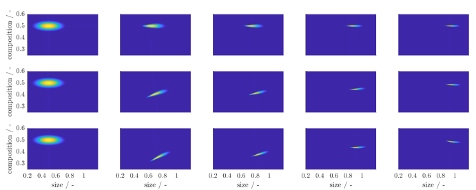
Figure 3: Evolution of the PSD for $G_{1}\equiv G_{2}$ (top row), $G_{1}\equiv 2G_{2}$ (middle row) and $G_{1}\equiv 5G_{2}$ (bottom row) from left to right. The predicted PSD focusing, denoted by the growth kinetics, clearly shows the strong ability of eMoM to capture this.

The first solution formula allows us to evaluate the particle distribution at any time, and disperse property, while the second enables the initial datum to be easily tracked over time, as only the disperse properties $\boldsymbol{x}$ within the support of the initial datum $q_{0}$ have to be evaluated. It is worth mentioning that whatever scheme is used to approximate the evolution of the concentrations over time, the solution formula can then be utilized to evaluate the PBE solution with high accuracy – keeping in mind that this is only true if the concentrations are approximated accurately enough. In Figure 3, the evolution of a PSD is depicted for two growth rate ratios, showing a clear change in the composition over process time.

5.1 Comparison with classical discretization schemes

We compare the numerical scheme derived here with state-of-the-art finite volume method schemes (FVM) [17, 8]. To enforce boundedness and numerical stability of the FVM, we consider the total variation diminishing schemes (TVD) [17] with a van-Leer limiter function enabling weighting between first and second order approximations of the growth term[18]. Figure 4 shows a numerical comparison between MD-eMoM and FVM. The newly derived MD-eMoM clearly outperforms FVM. First, it does not need to satisfy a CFL condition [19] because it relies on the solution of the characteristics. Second, MD-eMoM does not suffer from poor (coarse) discretization of the disperse property as only the support of the initial datum has to be discretized, see Figure 4.

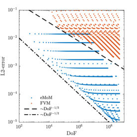
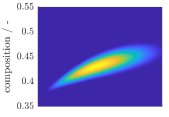
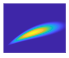
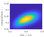
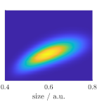
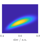
Figure 4: Left: Comparison of the $L^{2}$-error for the predicted evolution of the concentration between MD-eMoM and FVM for a large range of discretizations (DoF). One can clearly identify an order of $1/3$ with respect to the DoF for FVM and of $1/2$ for eMoM. Right: The number density function $q$ at $t=0.01$ for different DoF (from left to right, $10^{6}$ through $10^{7}$ to $10^{8}$), where the top and bottom row represent the solution of MD-eMoM and FVM, respectively. For coarse discretizations (small DoF), the FVM solution is diffusive. Furthermore, the whole domain in FVM needs to discretized though it is only partly used. By contrast, eMoM is non-diffusive and, by definition, only implicitly discretizes the support of the PSD for all process times.

6 Additional insights into Nanoparticle structure

In many applications, the inner-particle structure determines the product properties, e.g., the radial composition of gold (Au) and silver (Ag) in AuAg nanoalloys determine the optical properties [11]. Having the time evolution of the educt concentrations ${\boldsymbol{c}}$, we can also reconstruct the inner-particle composition for every particle in the number density function based on the characteristics. For a particle at time $t$ with initial disperse property $\boldsymbol{x}^{0}$, the composition $\mathcal{F}$ at every radial position $\boldsymbol{\xi^{\mathsf{c}}}(0,\boldsymbol{x}^{0},\tau)$ for $\tau\in[0,t]$ is given by:

$$\mathcal{F}_{\boldsymbol{x}^{0},t}\big{(}\boldsymbol{\xi^{\mathsf{c}}}_{\!\!\!1}(0,\boldsymbol{x}^{0},\tau)\big{)}=\frac{\boldsymbol{G}_{1}({\boldsymbol{c}}_{1}(\tau))}{\boldsymbol{G}_{1}({\boldsymbol{c}}_{1}(\tau))+\boldsymbol{G}_{2}({\boldsymbol{c}}_{2}(\tau))}.$$ (15)

This allows us to trace the evolution of the radial composition over process time and to characterize the properties of the final particle size distribution.
To demonstrate the potency of this unique analysis approach, we consider the seeded growth of gold-silver alloy NPs and investigate the effect of different growth rate ratios on the inner-particle structure (here optical properties). Under the assumption of radial symmetry, the optical properties can be numerically calculated by MIE Theory [20] (we use the MATLAB code of J. Schäfer[21]). As composition-dependent material properties, i.e., refractive indices, we interpolate the measured refractive index for gold-silver alloys by McPeak et. al. [22]. We prescribe the initial datum $q_{0}$ to be of uniform composition 0.5. Figure 5 (left) shows the inner-particle composition for a particle with size 7 nm after the solid formation process is finished. The different radial compositions due to the different growth rate ratios result in different extinction spectra, and thus optical properties, as seen in Figure 5 (right).

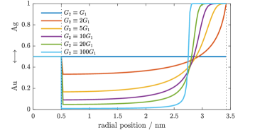
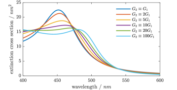
Figure 5: Radial composition (left) and the resulting extinction cross-section spectra (right) of AuAg nanoalloys for different growth rate ratios. The optical properties heavily depend on the radial distribution of Au-Ag. Note that all the particles have the same average fraction of Au-Ag, i.e., 0.5. For the sake of simplicity, the initial particle size distribution $q_{0}$, i.e., the seeds, was chosen as a Dirac-$\delta$ with a radius of $0.5$nm and a composition of $0.5$. For the growth rate ratios $1$ and $5$, the evolution of a full $q_{0}$ is depicted in Figure 3. The Dirac follows the same evolution.

7 Conclusion and Outlook

The multi-dimensional exact method of moment is an efficient way to approximate solutions of multi-dimensional population balance equations by relying on a fixed-point reformulation in terms of the driving forces – here the solute concentrations. The introduced numerical approach allows for highly accurate prediction of the evolution of multi-dimensional number density function, and the reformulation of the governing equations into a set of integro-differential equations results in markedly improved computational efficiency and numerical accuracy compared to state-of-the-art finite volume or finite element methods. Another advantage relates to process optimization, as the derived numerical scheme is differentiable by construction and thus derivatives with respect to process conditions can be computed by utilizing the implicit-function theorem.

Our numerical scheme can easily be extended to take into account the nucleation and growth of composite particles, as well as the formation of anisotropic particles[8]. Moreover, it is not limited to just one composition but can handle multiple compositions. A natural straightforward extension of the scheme would be implicit discretization of the fixed-point problem, resulting in an $n$-dimensional nonlinear system of equations for each time-step in Algorithm 1, ($n$ being the number of considered concentrations). Furthermore, the multi-dimensional exact method of moment idea can be coupled to fluid-flow, as already outlined in Bänsch et. al.[23] for the one-dimensional case.

References

• Pflug et al. [2020] L. Pflug, T. Schikarski, A. Keimer, W. Peukert, M. Stingl, emom: Exact method of moments—nucleation and size dependent growth of nanoparticles, Computers & Chemical Engineering 136 (2020) 106775.
• Murthy [2007] S. K. Murthy, Nanoparticles in modern medicine: state of the art and future challenges, International Journal of Nanomedicine 2 (2007) 129–141.
• Polavarapu and Liz-Marzán [2013] L. Polavarapu, L. M. Liz-Marzán, Towards low-cost flexible substrates for nanoplasmonic sensing, Physical Chemistry Chemical Physics 15 (2013) 5288–5300.
• Peukert et al. [2015] W. Peukert, D. Segets, L. Pflug, G. Leugering, Chapter one - unified design strategies for particulate products, in: G. B. Marin, J. Li (Eds.), Mesoscale Modeling in Chemical Engineering Part I, volume 46 of Advances in Chemical Engineering, Academic Press, 2015, pp. 1–81.
• Wawra et al. [2018] S. E. Wawra, L. Pflug, T. Thajudeen, C. Kryschi, M. Stingl, W. Peukert, Determination of the two-dimensional distributions of gold nanorods by multiwavelength analytical ultracentrifugation, Nature Communications 9 (2018) 1–11.
• Meincke et al. [2022] T. Meincke, J. Walter, L. Pflug, T. Thajudeen, A. Völkl, P. C. Lopez, M. J. Uttinger, M. Stingl, S. Watanabe, W. Peukert, et al., Determination of the yield, mass and structure of silver patches on colloidal silica using multiwavelength analytical ultracentrifugation, Journal of Colloid and Interface Science 607 (2022) 698–710.
• Lopez et al. [2022] P. C. Lopez, M. Uttinger, N. Traoré, H. Khan, D. Drobek, B. A. Zubiri, E. Spiecker, L. Pflug, W. Peukert, J. Walter, Multidimensional characterization of noble metal alloy nanoparticles by multiwavelength analytical ultracentrifugation, Nanoscale 14 (2022) 12928–12939.
• Braatz and Hasebe [2002] R. D. Braatz, S. Hasebe, Particle size and shape control in crystallization processes, in: AIChE Symposium Series, Citeseer, pp. 307–327.
• Schiele et al. [2023] S. A. Schiele, R. Meinhardt, T. Friedrich, H. Briesen, On how non-facetted crystals affect crystallization processes, Chemical Engineering Research and Design 190 (2023) 54–65.
• Keimer et al. [2018] A. Keimer, L. Pflug, M. Spinola, Existence, uniqueness and regularity of multi-dimensional nonlocal balance laws with damping, Journal of Mathematical Analysis and Applications 466 (2018) 18–55.
• Rioux and Meunier [2015] D. Rioux, M. Meunier, Seeded growth synthesis of composition and size-controlled gold–silver alloy nanoparticles, The Journal of Physical Chemistry C 119 (2015) 13160–13168.
• Dong and Koenig [2020] H. Dong, G. M. Koenig, A review on synthesis and engineering of crystal precursors produced via coprecipitation for multicomponent lithium-ion battery cathode materials, CrystEngComm 22 (2020) 1514–1530.
• Thanh et al. [2014] N. T. K. Thanh, N. Maclean, S. Mahiddine, Mechanisms of nucleation and growth of nanoparticles in solution, Chemical Reviews 114 (2014) 7610–7630.
• Schikarski et al. [2022a] T. Schikarski, M. Avila, W. Peukert, En route towards a comprehensive dimensionless representation of precipitation processes, Chemical Engineering Journal 428 (2022a) 131984.
• Schikarski et al. [2022b] T. Schikarski, M. Avila, H. Trzenschiok, A. Güldenpfennig, W. Peukert, Quantitative modeling of precipitation processes, Chemical Engineering Journal 444 (2022b) 136195.
• Keimer and Pflug [2017] A. Keimer, L. Pflug, Existence, uniqueness and regularity results on nonlocal balance laws, Journal of Differential Equations 263 (2017) 4023–4069.
• LeVeque [2002] R. J. LeVeque, Finite volume methods for hyperbolic problems, volume 31, Cambridge university press, 2002.
• Sweby [1984] P. K. Sweby, High resolution schemes using flux limiters for hyperbolic conservation laws, SIAM Journal on Numerical Analysis 21 (1984) 995–1011.
• Courant et al. [1928] R. Courant, K. Friedrichs, H. Lewy, Über die partiellen Differenzengleichungen der mathematischen Physik, Mathematische annalen 100 (1928) 32–74.
• Mie [1908] G. Mie, Beiträge zur Optik trüber Medien, speziell kolloidaler Metallösungen, Annalen der Physik 330 (1908) 377–445.
• Schäfer [2011] J.-P. Schäfer, Implementierung und Anwendung analytischer und numerischer Verfahren zur Lösung der Maxwellgleichungen für die Untersuchung der Lichtausbreitung in biologischem Gewebe, Ph.D. thesis, Universität Ulm, Ulm, Germany, 2011.
• McPeak et al. [2015] K. M. McPeak, S. V. Jayanti, S. J. Kress, S. Meyer, S. Iotti, A. Rossinelli, D. J. Norris, Plasmonic films can easily be better: rules and recipes, ACS photonics 2 (2015) 326–333.
• Bänsch et al. [2022] E. Bänsch, L. Pflug, T. Schikarski, Highly accurate and numerical tractable coupling of nanoparticle nucleation, growth and fluid flow, Chemical Engineering Research and Design (2022).