Interpretable and Robust AI in EEG Systems:
A Survey

Abstract

The close coupling of artificial intelligence (AI) and electroencephalography (EEG) has substantially advanced human-computer interaction (HCI) technologies in the AI era. Different from traditional EEG systems, the interpretability and robustness of AI-based EEG systems are becoming particularly crucial. The interpretability clarifies the inner working mechanisms of AI models and thus can gain user trust for transparent and ethical use of EEG systems. The robustness reflects the AI’s reliability against attacks and perturbations, which is essential for sensitive and fragile EEG signals. Thus the interpretability and robustness of AI in EEG systems have attracted increasing attention, and their research has achieved great progress recently. However, there is still no systematic survey of the AI-based EEG systems, making it challenging for researchers to fully grasp the state-of-the-art and emerging trends in this rapidly evolving field. In this paper, we present the first comprehensive survey on the interpretable and robust AI techniques for EEG systems. Specifically, we first introduce the background knowledge of EEG signals. Then we propose a taxonomy of interpretability by characterizing it into three types: backpropagation, perturbation, and rule-based methods. Moreover, we categorize the robustness mechanisms into four classes: noise and artifacts, human variability, data acquisition instability, and adversarial attacks. We conduct detailed analyses and comparisons for each category. Finally, we identify several key challenges for interpretable and robust AI in EEG systems and further discuss their future directions. This survey can provide valuable guidance for researchers to gain insights into the latest advancements and future trends in this field.

I Introduction

Electroencephalogram (EEG) provides valuable information about activities and states of the brain in a non-invasive way, being one of the active research areas in human-computer interaction (HCI). With the blossoming of recent artificial intelligence (AI) technologies, EEG systems have increasingly embraced the power of AI for various clinical, entertainment and social interaction applications. For example, sleep staging systems combine EEG signals with deep learning to assist physicians in rapid diagnosis [1]. Driver monitoring systems employ EEG-based deep neural networks (DNNs) to accurately detect driver fatigue to reduce the risk of car accidents [2]. Robotic arm control systems use DNNs to translate human thoughts (reflected by EEG signals) into control signals, helping the disabled perform basic tasks, such as drinking water or moving objects [3]. Although significant progress has been made by AI, the AI models (especially the deep learning-based ones) still remain unexplainable due to their black-box nature and are also susceptible to intentional or unintentional attacks, raising serious concerns for the interpretability [4, 5] and robustness [6] of AI in EEG systems.

Interpretability refers to understanding why and how the AI models make decisions and predictions. Specific to AI-based EEG systems, the interpretability allow researchers to gain insights into EEG dynamics and the link between brain states and cognitive functions, and also make it easier to identify potential biases and failure modes of EEG systems. From another point of view, the interpretability can foster user trust and acceptance of EEG systems, enabling users to build confidence in the validity and value of EEG systems.

Robustness refers to the degree to which the decisions and predictions of AI models are free from attacks and perturbations. Unlike traditional HCI data such as image, audio and video, EEG data derived from brain tends to be noisy and variable across individuals, resulting in a lower signal-noise ratio (SNR). This is because EEG signals are easily interfered by biological and environmental artifacts(e.g., muscle movements, eye blinks, heartbeat, electrical devices, etc.), and the same stimuli also evoke different EEG responses in different people which has unique neural rhythms.

In recent years, there has been a surge of research interest within the academic community aimed at enhancing the interpretability and robustness of AI-based EEG systems. Fig. 1 shows the year-by-year number of papers on these topics. We collect research papers employing the keywords “interpretable”, “interpretability”, “explainable”, “explainability”, “robust” and “robustness”, in conjunction with “EEG”. The selection of these papers spans from 2018 to the present and comprises publications from diverse sources such as arXiv, conference proceedings and academic journals. The data in Fig. 1 reveals that more than 60% of these papers were published within the past two and a half years, indicating the growing popularity of this field.

While the interpretability and robustness in AI based EEG systems have raised serious concerns, and despite tremendous efforts made by researchers to address them, an exhaustive survey summarizing the state of knowledge on these two critical topics remains lacking. There are surveys on interpretable and robust AI in general, but none of them specifically focuses on EEG Systems. To fill this gap, in this paper we present a systematic survey covering the following aspects.

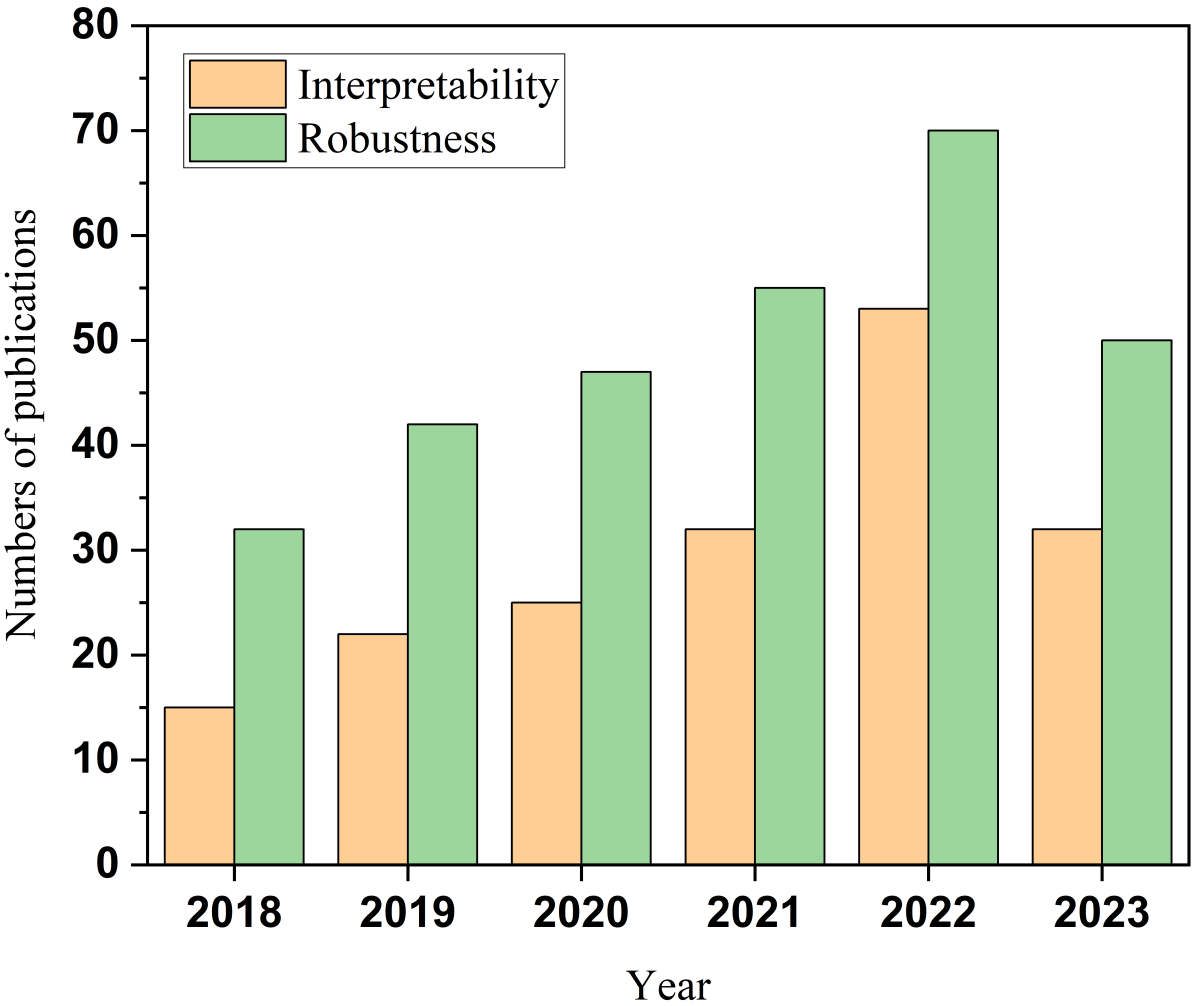
(a)

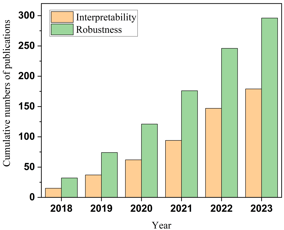
(b)

Figure 1: The increasing trend of interpretable and robust AI-related publications in recent six years. (a) The annual number of published papers related to interpretable and robust AI in EEG systems since 2018. (b) The cumulative number of published interpretable and robust-related papers since 2018.

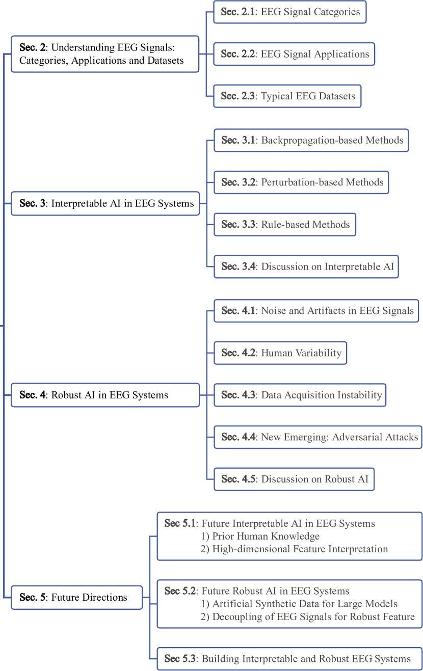
Figure 2: Organization of this survey paper.

We first introduce the background of EEG signals from the EEG categories, EEG applications and EEG datasets. We then elaborate the interpretability and robustness of AI in EEG systems, respectively. For the interpretability, we classify the interpretable AI into three types from the implementation perspective of interpretability methods. The first type is post-hoc methods based on backpropagation, which obtains the contribution of the features to results by backpropagating the prediction results. The second type is perturbation-based methods that explain initial models using local models trained with data perturbation. The last type is rule-based methods, and it applies models based on logical rules to make predictions. For the robustness, we categorize the robust AI into four classes: signal-component-related, subject-related, device-related, and the latest adversarial-attack-related challenges, covering all threats to the stability and security of AI-based EEG systems in practical applications. Within each category, we summarize the common features and shared methodologies, describe representative works, and analyze their differences. Finally, we discuss the potential directions for future research and propose practical suggestions. The tree diagram of the paper structure is illustrated in Fig. 2.

The contributions of this survey are as follows:

• This is the first comprehensive survey focusing on the interpretability and robustness of AI in EEG systems.

• We propose a novel taxonomy of interpretability and robustness for EEG systems.

• We summarize and highlight the emerging and most representative interpretable and robust AI works related to EEG systems.

• We discuss some open problems and promising directions for future EEG systems.

• We maintain an ever-evolving list of papers on the interpretability and robustness of AI in EEG systems, with frequent updates to ensure its comprehensiveness and timeliness. The list goes here: https://github.com/xinliangzhou/Survey/blob/main/Paper_List.md

II Understanding EEG Signals:
Categories, Applications and Datasets

In this section, we provide an overview of the EEG paradigms, including EEG signal categories, EEG signal applications and typical EEG datasets. The EEG paradigm is a widely used approach in the field of BCI, and it involves measuring the brain’s electrical activity through electrodes placed on the scalp. Compared with other paradigms in BCI, such as the ECoG paradigm [7], the advantages of the EEG paradigm include its non-invasive nature, high temporal resolution, and relative ease of use. However, it has poor spatial resolution and is susceptible to interference from external sources such as muscle activity. Despite these limitations, the EEG paradigm continues to be a valuable tool in developing BCI technology.

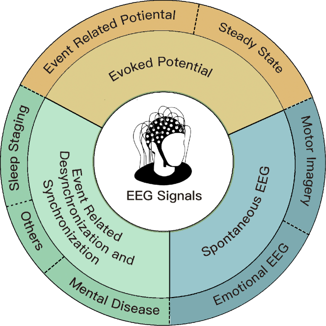
Figure 3: Summary of EEG Signal Categories.

II-A EEG Signal Categories

EEG signals fall into three general categories: spontaneous EEG, evoked potentials, and event-related desynchronization/synchronization (ERD/ERS). The spontaneous EEG do not involve external stimuli presented to subjects, while the evoked potentials elicit the subjects’ EEG responses to specific external stimuli. In contrast, the ERD/ERS is stimuli-irrelevant, only reflecting subjects’ mental activities. The EEG signal categories are shown in Fig. 3.

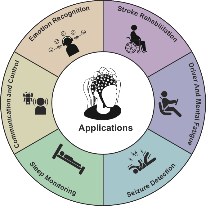
Figure 4: Typical EEG Applications.

II-A1 Spontaneous EEG

The most widely used EEG, in general, is spontaneous EEG. It refers to the measurement of brain waves obtained without external stimuli. Some common spontaneous EEG signals are obtained from the scenarios where test subjects are engaged in experiencing fatigue and sleeping, suffering from a brain disorder (e.g., Autism, Seizure), and performing motor imagery (MI) tasks [8].

II-A2 Evoked Potentials

Evoked Potentials (EPs), also called evoked responses, are EEG signals elicited by non-spontaneous event stimuli. Depending on different kinds of stimuli, there are two forms of EPs signals: event-related potentials (ERPs) and steady-state evoked potentials (SSEPs). The ERPs record the EEG signals elicited by specific and isolated stimulus events. While the SSEPs can reflect subjects’ perception of pressure, touch, temperature and pain. On this basis, both ERPs and SSEPs contain somatosensory, auditory, and visual potentials according to the subjects’ senses. All EPs signals, such as $P300$ [9], rapid serial visual presentation (RSVP) [10], and error-evoked potentials, are more robust than spontaneous signals because the amplitude and frequency of EPs are typically higher.

II-A3 Event-Related Desynchronization and Synchronization

The ERD/ERS reflects a relative power decrease/increase of EEG in a specific frequency band during physical motor executions and mental activities. The ERD/ERS does not require any external stimuli. However, to gather high-quality ERD/ERS signals, participants must undergo lengthy training that may last several weeks. In addition, the ERD/ERS signals are prone to fluctuate with different participants and thus have low stability.

TABLE I: Summary of public datasets used in EEG systems.

Task	Dataset	Physiological Signal	Subject Number	Subject Age
Emotion Recognition	Deap [11]	EEG, EMG, EOG, BVP	$32$	$19-37$ (Mean $26.9$)
	SEED [12]	EEG	$15$	Mean $23.27$
	SEED-IV [13]	EEG	$15$	$20-24$
	SEED-V [14]	EEG, SMI	$20$	N/A
	Dreamer [15]	EEG, ECG	$23$	$20-33$
	HCI-Tag [16]	EEG, ECG, GSR, TEMP, RSP	$30$	$19-40$ (Mean $26.1$)
	ASCERTAIN [17]	EEG, ECG, GSR	$58$	Mean $30$
	AMIGOS [18]	EEG, ECG, GSR	$40/37$	N/A
	Enterface 06 [19]	EEG, fNIRS	$16$	N/A
	Imagined Emotion [20]	EEG	$31$	$18-38$
Fatigue Detection	MEDT [21]	EEG	$27$	$22-28$
	DDDE [22]	EEG	$13$	$44.5\mp 18.8$
	FatigueSet [23]	EEG, ECG, PPG, EDA, TEMP	$12$	N/A
Seizure Detection	CHB-MIT [24]	EEG	$23$	$1.5-22$
	Bonn University [25]	EEG	$10$	N/A
	Freiburg Seizure [26]	EEG	$21$	Adults and Children
	Helsinki University [27]	EEG	$79$	Infants
	EPILEPSIAE [26]	EEG	$275$	N/A
	Temple University [28]	EEG	$80$	$6-56$
	NMT [29]	EEG	N/A	$1-90$
Sleep Monitoring	Sleep-EDF [30]	EEG, EMG, EOG	$197$	$18-90$
	SHHS [31]	EEG, EMG, ECG, EOG	$6441$	Above $40$
	MASS [32]	EEG, EMG, ECG, EOG	$200$	$18-76$
	ISRUC [33]	EEG, EMG, ECG, EOG	$118$	Adults and Children
	HMC [34]	EEG, EMG, EOG	$105$	$20-80$
	CAP Sleep [35]	EEG, ECG, EOG	$102$	$18-70$
	Sleep Cassette [36]	EEG, EOG, EMG	$100$	$18-65$
	SIESTA [37]	EEG, EOG, EMG, ECG	$72$	$18-80$
Motor Imagery	BCI IV 2a* [38]	EEG, EOG	$9$	N/A
	BCI IV 2b* [38]	EEG, EOG	$9$	N/A
	OpenMBI [39]	EEG	$54$	$24-45$
	Stroke [40, 41]	EEG	$21$	Mean $54.2$
	MOABB [42]	EEG	$104$	$18-55$

II-B EEG Signal Applications

EEG signals have various applications. We list the six most typical applications shown in Fig. 4.

II-B1 Sleep Monitoring

Sleep monitoring plays a crucial role in the early diagnosis and intervention of sleep-related diseases. According to the sleep staging criteria proposed by the American Academy of Sleep Medicine (AASM) [43], the complete sleep process can be divided into three stages: wakefulness (W), non-rapid eye movements (NREMs), and rapid eye movements (REMs). Different sleep stages are reflected in different prominent waveforms in EEG signals. For example, spindles and K-complex waveforms are prominent features in the NREMs stage [44]. To save manpower and time, employing EEG signals for automatic sleep monitoring has gradually become a hot research topic [45, 46, 47].

II-B2 Seizure Detection

The characteristics of seizure activities can be observed from EEG signals, which provide essential information about the type and severity of the seizure and help identify the location of the seizure focus in the brain (e.g., temporal lobe) [48, 49]. The EEG signals are crucial for developing effective treatment plans and monitoring the patient’s health condition.

II-B3 Fatigue Detection

EEG signals can be used for detecting and monitoring fatigue, such as driver fatigue [50, 51] and mental load fatigue. One common way is through spectral power analysis, for which the changes in the power of different frequency bands can be used as fatigue indicators. Another way is to analyze the ERPs. When fatigue happens, the amplitude of certain ERPs (e.g., $P300$) will decrease [52]. EEG signals can also be combined with other techniques, such as eye tracking and reaction time tests, providing a more complete picture of the cognitive and neural changes associated with fatigue.

II-B4 Communication and Control

EEG signals representing human intent can be decoded into language or control signals used to communicate with people or intelligent devices. A typical application is the $P300$ speller, which enables users to type without any motor systems and converts their intention into text [9, 53, 54]. Besides, some intelligent environment stuff can be linked to and controlled by EEG systems, e.g., assistive robots in smart homes. These applications can be achieved by detecting SSVEP owing to the advantages of less training time, excellent recognition performance, and high information translation rate (ITR) [55, 56]. Current research in this scenario focuses mainly on controlling robots [57, 58, 59], wheelchairs [60, 58], etc.

II-B5 Emotional Recognition

EEG systems can be applied to assess and understand changes in the brain related to mental and physical states [61, 62, 63]. Studies have shown differences in the activity of specific brain regions, such as the amygdala and prefrontal cortex, when a person is experiencing fear or happiness. Activities in these brain regions are directly reflected in the related EEG signals, which could be applied to mental health [64], cognitive psychology [65], and affective computing research [66, 5].

II-B6 Stroke Rehabilitation

Stroke has a high mortality rate and leads to long-term disability in up to $50\%$ of survivors. Therefore, motor rehabilitation is a top priority for post-stroke treatment [67]. Unlike traditional stroke rehabilitation treatments, EEG systems do not rely on patients’ residual motor ability. In contrast, EEG systems create a direct communication pathway between the brain and an external device [68], bypassing the traditional neuromuscular pathway. During EEG system-assisted rehabilitation, the system collects the patient’s EEG signals and then decodes the patients’ motor intentions into commands through signal processing. These commands drive the robotic device to move the patient’s paralyzed limb to complete the rehabilitation exercise. Studies have reported motor cortex activation in patients who underwent EEG Systems-based rehabilitation and statistically significant improvements in patients’ motor abilities during subsequent motor assessments [69, 70].

II-C Typical EEG Datasets

The selection and utilization of datasets is a critical foundation of physiological signal processing, greatly affecting the interpretability and robustness of derived conclusions. Table I summarizes the public EEG datasets employed for various tasks, including emotion recognition, fatigue detection, seizure detection, sleep monitoring and motor imagery.

For example, the emotion recognition task engages datasets such as Deap [11], Dreamer [15], and ASCERTAIN [17], which incorporate various physiological signals, encompassing EEG, Electromyography (EMG), Electrocardiogram (ECG), Galvanic Skin Response (GSR), Temperature (TEMP), and Respiratory (RSP). These datasets cater to various age demographics and compile a substantial number of subjects, thereby augmenting the robustness of the analytic methodologies applied. Likewise, fatigue detection and seizure detection tasks leverage diverse datasets, underscoring the resilience and adaptability of the ensuing models.

Differently, sleep monitoring and motor imagery domains utilize multiple datasets collated from a wide demographic range, reinforcing the inferred models’ broad applicability. The comprehensive nature of these datasets buttresses the interpretability of the findings by providing a detailed understanding of the behavior of different physiological signals under an array of conditions.

The broad spectrum of datasets outlined in Table I underscores the extensive application of these tasks across various ages and subject populations, highlighting the inherent robustness of these approaches. Besides, these datasets contribute to the interpretability by fostering a nuanced and comprehensive understanding of the field, thus improving the transparency in physiological signal processing.

TABLE II: Summary of Interpretable AI in EEG Systems.

Interpetability Categories	Methods	Coverage	Explanation Type	Representative Works
Backpropagation-based Methods	LRP	Local/Global	Attribution	[71, 72, 73, 74, 75]
	DeepLIFT	Local/Global	Attribution	[76, 77, 78, 79, 80]
	CAM	Local	Attribution	[50, 81, 82, 83, 84]
	Grad-CAM	Local	Attribution	[85, 86, 87, 88, 89]
Perturbation-based Methods	LIME	Local	Attribution	[90, 91, 92, 93, 94]
	SHAP	Local	Attribution	[78, 95, 96, 97, 98]
Rule-based Methods	RF	Global	Decision Rules	[99, 100, 101, 102, 103]
	FIS	Global	Fuzzy Rules	[104, 105, 106, 107, 108]
BS	Global	Bayesian Rules	[109, 110, 111, 112, 113]

III Interpretable AI in EEG Systems

AI interpretability refers to explaining the decisions and actions of AI models in a manner that humans can understand. For interpretable AI in EEG systems, it means the internal logic and workings of AI models conform to physiological principles. For example, in motor imagery (MI) tasks, the EEG signals that contribute to predictions are derived from electrodes around the motor cortex, as depicted in Fig. 5.

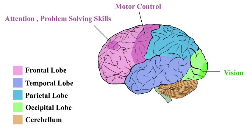
Figure 5: Key brain regions related to the motor imagery task. These include the frontal lobe for cognitive skills and motor function, the temporal lobe for sensory input processing, the parietal lobe for sensory information integration, the occipital lobe for vision, and the cerebellum for coordination of voluntary movements. Each region contributes to the successful execution of the task.

Interpretability is essential for EEG systems because it assesses whether the AI model has learned physiologically meaningful features. Foremost, interpretability allows checking whether the predictive logic of AI models conforms to specific proven physiological rules, since the predictive accuracy scores of the AI models can be deceptive. For example, in MI tasks, the model making decisions may pay more attention to the noises generated by subjects’ involuntary muscle movements rather than EEG signals that truly originate from cranial nerve movements. Furthermore, interpretability methods can uncover patterns that inform brain signal research. For example, when predicting subjects’ sleep states, models identified that the signals of peripheral EEG channels generated by regular eye movements during deep sleep are highly correlated with sleep status [114], even though these EEG signals had long been overlooked.

After a thorough review of existing literatures, we divide the interpretability methods applied in EEG systems into three categories from the perspective of the implementation: backpropagation-based methods, perturbation-based methods and rule-based methods. We summarize the interpretability categories and their representative works in Table II.

Type and Coverage of interpratable AI in EEG Systems: In EEG systems, the interpretability of AI models can be broadly categorized as either local or global, influenced by feature attribution or logic rules. Local interpretability aims to explain individual predictions by illuminating why a model correlates a specific EEG pattern with a particular condition. Techniques like Layer-wise Relevance Propagation (LRP) [115], DeepLIFT [116], Class Activation Mapping (CAM) [117], Gradient-weighted Class Activation Mapping (Grad-CAM) [118], Local Interpretable Model-Agnostic Explanations (LIME) [119], and Shapley Additive Explanations (SHAP) [120] provide local interpretability.

In contrast, global interpretability illuminates the overall behavior of a model, revealing how it operates across multiple instances. Methods like random forest (RF) [121], fuzzy inference system (FIS) [122] and Bayesian system (BS) [123] are frequently utilized for the global interpretability.

Feature attribution, assigning importance values to input features for a model’s decision, is prevalent in methods such as LRP, DeepLIFT, CAM, Grad-CAM, LIME and SHAP, potentially highlighting key brain activity patterns. Meanwhile, logic rules that provide clear criteria for classifying EEG data conditions are also used in RF, FIS and BS.

The explanation type (attribution or logic rule) and interpretability scope (local or global) provide unique and crucial insights into AI decision-making in EEG systems. The selection depends on the required level of interpretability and the most appropriate explanation type for the given data and task.

III-A Backpropagation-based Methods

Backpropagation-based methods decompose the model predictions by first backpropagating the gradients from the predictions into input feature space and then visualizing the weights of these features (e.g., time-frequency patterns and electrode regions) in raw EEG signals that contribute to predictions.

III-A1 Layer-wise Relevance Propagation (LRP)

LRP [115] provides insight into the neurophysiological phenomena behind EEG models’ predictions by backpropagating results. The LRP aims to determine the contribution (measured by the relevance value) of individual elements within the input signal (corresponding to each sample point of the EEG signal) to the output prediction. It allows EEG models to integrate temporal information and brain-topography-related spatial information by producing heatmaps.

To implement the LRP, a neural network like a convolutional neural network (CNN) is first be trained to process EEG signals. Let $R^{(l)}_{i}$ denotes the relevance value of neuron $i$ in layer $l$ ($l=1,2,\ldots,L$). At the output layer (i.e., $l=L$), the relevance value is equivalent to the model’s predicted score:

$$R_{i}^{(L)}=f_{i},$$ (1)

where $f_{i}$ is the activation value of neuron $i$ in the output layer of the neural network. For each layer $l$, the backpropagation is used to propagate $R^{(l)}_{i}$ to the subsequent layer, $R^{(l-1)}_{j}$. In the LRP, this process is defined as

$$R_{j}^{(l-1)}=\sum_{i}\frac{f_{j}^{(l-1)}w_{ji}^{(l)}}{z_{i}^{(l)}}R_{i}^{(l)},$$ (2)

where $f_{j}^{(l-1)}$ represents the activation value of neuron $j$ in layer $(l-1)$, $w_{ji}^{(l)}$ denotes the weight between neuron $i$ in layer $l$ and neuron $j$ in layer $(l-1)$, and $z^{(l)}_{i}=\sum_{j}f_{j}^{(l-1)}w_{ji}^{(l)}$ denotes the sum of the inputs to neuron $i$ in layer $l$.

Backpropagating through each layer allows us to calculate the relevance values for every sample point in the input layer (i.e., the original EEG signal). A higher relevance value indicates that the data contributed more to the prediction, while a lower value indicates less contribution. Visualizing these relevance values reveals how the neural network extracts useful information from EEG signals. This offers insights to improve neural network models or understand brain signals more thoroughly.

The LRP reveals whether the models focus on task-relevant EEG signals. Ellis et al. [72] used the LRP to generate heatmaps highlighting the local and global signals. The heatmaps show that the local signals with higher relevance values are highly related to the sleep state of the human brain, matching neurophysiological expectations. Similarly, the LRP can clarify the contributions of noise and neurophysiological factors. Nagarajan et al. [73] applied LRP to select the high contributing EEG channels in MI tasks, confirming that the model indeed learns features from the electrodes at action-related brain regions.

The LRP also reveals how EEG signals from different brain dimensions correlate with model decisions over time. Sturm et al. [74] used the LRP to track how a DNN’s attention shifted between feature regions during action switching in MI tasks, revealing the physiological principles underlying the model predictions. Moreover, Wang et al. [124] and Bang et al. [71] leveraged the LRP to explain 3D-CNN model predictions, for which the heatmaps simultaneously highlighted the contributions of frequency ranges, time intervals and spatial locations of relevant signals.

III-A2 Deep Learning Important Features (DeepLIFT)

DeepLIFT aims to check if the model’s decisions align with known neurophysiological phenomena, and provide guidance for finding generalizable EEG features. Similar to LRP, the DeepLIFT uses backpropagation to calculate how each input feature correlates with the model prediction for each trial.

The DeepLIFT is based on reference activation, enabling comparison of a feature’s importance against a predefined reference point. Its core principle is to calculate a contribution score for each input feature. The contribution score can be computed using the following equation:

$$C_{i}=(f_{i}-f_{i}^{0})\times\frac{\partial y}{\partial f_{i}},$$ (3)

where $C_{i}$ denotes the contribution score for feature $i$, $f_{i}$ represents the actual activation of feature $i$, $f_{i}^{0}$ signifies the reference activation for feature $i$, $\frac{\partial y}{\partial f_{i}}$ denotes the gradient of the output with respect to the activation of feature $i$.

For the DNNs composed of multiple layers, the chain rule is employed to compute the contribution score for each input feature. The chain rule for DeepLIFT can be expressed as

$$C_{i}=\sum_{j}C_{i,j}=\sum_{j}\frac{\partial f_{j}}{\partial f_{i}}C_{j},$$ (4)

where $C_{i,j}$ indicates the contribution score of feature $i$ to feature $j$, $\frac{\partial f_{j}}{\partial f_{i}}$ denotes the gradient of the activation of feature $j$ with respect to the activation of feature $i$, and $C_{j}$ represents the contribution score for feature $j$.

The most common application of the DeepLIFT method in EEG systems is to verify whether the prediction logic of models conforms to physiological principles. For example, Lawhern et al. [76] used the DeepLIFT to prove that their proposed EEGNet can learn to focus on EEG channels near task-related brain regions in different EEG classification tasks. Similarly, Ju et al. [125] used the DeepLIFT to interpret the spatiotemporal frequency information learned by their Tensor-CSPNet in MI tasks, and found it match the key frequency components existing in the left and right hands.

On the other hand, the DeepLIFT can discover certain feature patterns from model predictions to guide brain research. For seizure detection, the high gamma frequency is known to be a key feature for distinguishing pre-ictal and inter-ictal segments. However, Gabeff et al. [77] interpreted the models using DeepLIFT, revealing that some low amplitude patterns were also detected as ictal. This finding complements the established conclusion, and verifies that the resting EEG features can also be helpful, providing counter-balancing information for seizure detection.

III-A3 Class Activation Mapping (CAM)

CAM is a technique that produces heatmaps by visualizing the importance of each input feature in the final classification decision. For EEG systems, the input features are often the EEG signals from multiple channels and time points. To describe the CAM method mathematically, let $f_{k}(x)$ denote the activation of the $k$-th feature map in the last convolutional layer of the network, given an input $x$. The class-specific weights $w_{c}^{k}$ for class $c$ are learned during the training process. The class activation map for class $c$ can be computed as

$$M_{c}(x)=\sum_{k}w_{c}^{k}\cdot f_{k}(x),$$ (5)

where $M_{c}(x)$ represents the heatmap for class $c$. This heatmap can be visualized as an overlay on the input EEG signals, highlighting the most relevant spatial and temporal features that contribute to the final classification decision.

To obtain the final classification score, the global average pooling (GAP) layer is applied on the feature maps, and then a softmax activation function is used to generate the probability distribution over classes:

$$p_{c}(x)=\frac{e^{S_{c}(x)}}{\sum_{c=1}^{C}e^{S_{c}(x)}},$$ (6)

where $S_{c}(x)=\sum_{i}\sum_{j}f_{k}^{c}(x)_{i,j}$ is the sum of the activation values of the $k$-th feature map for class $c$, and $C$ denotes the total number of classes.

CAM analysis connects the deep-layered features to the biologically meaningful features. In the work of Cui et al. [50], the features from the last convolutional neural network layer were traced back to the bursts in the $\theta$ band and the spindles in the $\alpha$ band, which strongly relate to drowsiness. Similarly, Yildiz et al. [81] analyzed the seizure detection model using CAM, and found that low-frequency EEG signals are critical for distinguishing seizures.

III-A4 Gradient-weighted Class Activation Mapping (Grad-CAM)

Grad-CAM extends the CAM approach by considering the gradient information flowing into the last convolutional layer of the network, offering a more precise and high-resolution visualization of relevant features in AI-based EEG systems. The Grad-CAM method computes the importance weight $\alpha_{c}^{k}$ for the $k$-th feature map with class $c$ in the last convolutional layer as follows:

$$\alpha_{c}^{k}=\frac{1}{Z}\sum_{i}\sum_{j}\frac{\partial S_{c}(x)}{\partial f_{k}(x)_{i,j}},$$ (7)

where $Z$ is the total number of spatial locations in the feature map, and $\frac{\partial S_{c}(x)}{\partial f_{k}(x){i,j}}$ denotes the gradient of the class score $S_{c}(x)$ with respect to the activation $f_{k}(x)_{i,j}$ at the spatial location $(i,j)$. The Grad-CAM heatmap for class $c$ can then be computed as

$$M_{c}^{\mathrm{Grad}}(x)=\mathrm{ReLU}\left(\sum_{k}\alpha_{c}^{k}\cdot f_{k}(x)\right),$$ (8)

where ReLU is the rectified linear unit function, ensuring that only positive contributions are considered. Compared to the CAM, the Grad-CAM gives a more nuanced understanding of how the model behaves, since it takes into account both the positive and negative influences of the input features.

The Grad-CAM have been utilized to provide insight into the features learned by classifiers. Fei et al. [83] revealed that higher frequency bands are particularly useful for emotion recognition. Jonas et al. [126] identified key EEG features for prognostication in comatose patients after cardiac arrest. Similarly, Aslan et al. [127] used the Grad-CAM to visualize model outputs and clarify the relationship between frequency components in seizure patients versus healthy individuals. Additionally, applying Grad-CAM for channel selection can enhance decoding efficacy and achieve an optimal balance between model performance and channel utilization [86].

III-B Perturbation-based Methods

Perturbation-based methods perturb individual EEG samples and observe the impact on subsequent network neurons and predictions, trying to reveal correlations between samples and model outputs. Similar to backpropagation-based methods, they are also post-hoc methods that interpret the models by attribution. However, the perturbation-based methods are model-agnostic, building local models to approximate the predictions of the original models based on perturbed inputs. In other words, the local models establish the connection between biological features and original model predictions.

III-B1 Interpretable Model-agnostic Explanations (LIME)

LIME explains target model predictions by approximating them locally with interpretable models. To be specific, the LIME approximates the complex model’s behavior near a specific input point $x$ using a simple and locally linear model, which quantifies the contribution of individual elements within the input signal to the prediction $f(x)$. The original input x is perturbed to create similar inputs $x_{i}$ with $i=1,2,\ldots,N$, and their corresponding predictions $f(x_{i})$ are obtained from the trained model. Weights $w_{i}$ for the perturbed inputs inputs $x_{i}$ are computed using an exponential kernel

$$w_{i}=\exp\left(-\frac{d_{i}^{2}}{\sigma^{2}}\right),$$ (9)

where $d_{i}$ denotes the distances between the $x$ and $x_{i}$, and $\sigma$ is a scaling factor.

The simple linear model (e.g., linear regression) is then trained using the perturbed inputs $x_{i}$, predictions $f(x)$, and weights $w_{i}$. The coefficients $\beta_{i}$ of this simple linear model represent the contributions of each sample point in the input signal to the output prediction:

$$f(x)\approx\sum_{i=1}^{N}\beta_{i}x_{i},$$ (10)

Visualizing these feature contributions provides insights into how the model processes EEG signals and extracts relevant information. This can guide researchers to improve neural network models or interpret brain signals more comprehensively.

Locally interpretable models offer a direct way to map initial model predictions onto EEG features. Giudice et al. [90] used local models to explain DNN predictions of voluntary/involuntary blinks, revealing that the peaks and troughs in signals correspond to voluntary and involuntary eye blink behaviors, respectively. Similarly, Alsuradi et al. [91] also utilized the LIME to explain active/inactive action predictions, and find that the action trial can be identified as active for strong desynchronization in the $\alpha$ and $\beta$ bands, and passive for the synchronization in those bands.

Some models, containing specialized layers like SAGpooling, impede the visualization of feaure contributions through backpropagation. To tackle this issue, Xu et al. [92] applied the LIME to construct local interpretability models for the domain adversarial graph attention model (DAGAM). They identify that the symmetry of EEG activities between the left and right hemispheres is a critical feature of neutral emotions.

III-B2 Shapley Additive Explanation Values (SHAP)

SHAP quantifies the contribution of each input features to prediction based on the Shapley values from game theory. The Shapley value refers to the marginal contribution of the EEG feature, which is the difference between prediction results before and after the feature is added. The SHAP value for feature $i$ in a model $f$ is defined as

$$\phi_{i}(f)\!=\!\sum_{S\subseteq N\backslash\{i\}}\frac{|S|!(|N|\!-\!|S|\!-\!1)!}{|N|!}[f(S\cup\{i\})\!-\!f(S)],$$ (11)

where $N$ is the set of all input features, $S$ is a subset of features without feature $i$, and $|S|$ denotes the cardinality of $S$. The term $f(S\cup\{i\})-f(S)$ represents the marginal contribution of feature $i$ when added to the subset of features $S$.

SHAP values have three key properties: local accuracy, missingness, and consistency. Local accuracy ensures that the sum of SHAP values for each input feature and the expected model output equals the model prediction for a specific instance. Missingness idictates that if a feature is missing or has no impact on the model prediction, its SHAP value will be zero. Consistency guarantees that if a feature contributes more in a new model compared to an old one, the SHAP value of that feature should not decrease.

The SHAP is often utilized to explain complex AI models in EEG systems. Tahmassebi et al. [78] constructed a real-time DNN model to monitor patients’ eye states. To ensure model interpretability in practical scenarios, they employ the SHAP to build locally interpretable models that reveal the relationship between EEG features and the eye state. Raab et al. [95] also used the SHAP to explain the feature contributions of initial models, which are DNN models of different dimensions ($1$-D and $3$-D) for seizure detection.

TABLE III: Comparison of different interpretability methods in EEG Systems.

	Backpropagation-based Method	Perturbation-based Method	Rule-based Method
Mechanism	Analyze the feature contribution by backpropagating the gradients from predictions.	Explain the original model’s behavior with local surrogate models.	Explain model using specific logic rules
Explanation Stage	Post-hoc	Post-hoc	Ante-hoc
Model Dependence	Model-specific	Model-agnostic	Model-agnostic
Flexibility	Low	High	High
Application Scenario	Differentiable models	Tolerable of high computational costs	Availability of priori knowledge
Limitation	Gradient dependency; Narrow applicability	Computationally intensive; Prone to overfitting	Oversimplify complex EEG systems; Require domain expertise

III-C Rule-based Methods

Unlike post-hoc interpretability methods which use feature contributions as the explanation, the rule-based methods apply particular logic rules, such as decision rule, fuzzy rule, Bayesian rule, as the interpretations of the EEG systems, resulting in high interpretability.

III-C1 Random Forest (RF)

RF is an rule-based method based on the “IF-THEN-ELSE” logic rule (i.e., decision rule). The interpretability of RF arises from two main aspects: feature importance and decision paths.

Feature Importance: Feature importance in RF is typically calculated using the Gini importance or mean decrease impurity (MDI). For each feature $i$ derived from the EEG signals, the Gini importance $I_{G}(i)$ is given by

$$I_{G}(i)=\sum_{t\in T_{i}}\frac{n_{t}}{n}\left(1-\sum_{c=1}^{C}p_{tc}^{2}\right),$$ (12)

where $T_{i}$ represents the set of nodes in the RF that split on feature $i$, $n_{t}$ is the number of samples reaching node $t$, $n$ is the total number of samples, $C$ is the number of classes, and $p_{tc}$ is the proportion of samples with class $c$ in node $t$. The Gini importance measures the decrease in node impurity, which is weighted by the probability of reaching each node. The features of the EEG signals can be ranked based on their Gini importance, so that the most relevant features (also the most relevant EEG signals) contributing to the model’s decision-making process can be identified.

Decision Paths: RF consists of multiple decision trees, each of which is trained on a bootstrapped sample of the original data. The decision path of an instance in a tree is the sequence of nodes from the root to a leaf node, which corresponds to the class assigned by the tree.

RF model interpretability can be achieved by analyzing decision paths for an instance across all trees. This reveals common patterns and rules leading to predictions, providing insights into the decision-making process.

Visualizing feature importance and decision paths provides a deeper understanding of how input EEG signals relate to model predictions, and can aid model refinement and more comprehensive brain signal interpretation. For example, Abdulhay et al. [128] employed the RF to classify the Shannon entropy of instantaneous values associated with each intrinsic mode function (IMF), directly responding to the association between the instantaneous amplitudes and frequencies of the IMF and seizures. Li et al. [129] followed a similar approach for seizure classification. The difference is that the authors classify the electrodes directly by RF to find the seizure onset zone (SOZ).

III-C2 Fuzzy Inference System (FIS)

FIS is a computational framework based on the fuzzy set theory, fuzzy logic or fuzzy reasoning. It offers inherent interpretability by using human-readable rules and transparent reasoning processes.

A typical FIS consists of four main components: fuzzification, fuzzy rule base, fuzzy inference engine, and defuzzification. The fuzzification involves converting crisp input values into fuzzy sets using membership functions. For each input variable $x_{i}$, a membership function $\mu_{A_{i}}(x_{i})$ is used to determine the degree of membership of $x_{i}$ to the fuzzy set $A_{i}$:

$$\mu_{A_{i}}\left(x_{i}\right):x_{i}\rightarrow[0,1],$$ (13)

where $\mu_{A_{i}}(x_{i})$ represents the degree of membership of $x_{i}$ to the fuzzy set $A_{i}$.

The fuzzy rule base is a collection of human-readable “IF-THEN” rules that describe the relationships between input and output fuzzy sets. A fuzzy rule can be expressed as:

where $x_{i}$ are the input variables, $A_{ki}$ and $B_{k}$ are fuzzy sets, and $R_{k}$ represents the $k$-th fuzzy rule.

The fuzzy inference engine combines the fuzzified input values and fuzzy rules to produce fuzzy output sets. The firing strength or weight $w_{k}$ of each rule $R_{k}$ is computed as the product of the membership degrees of the input values to their corresponding fuzzy sets:

$$w_{k}=\prod_{i=1}^{n}\mu_{A_{ki}}\left(x_{i}\right),$$ (15)

The fuzzy output sets are then generated by aggregating the weighted consequent fuzzy sets $B_{k}$:

$$B_{k}^{\prime}(x)=w_{k}\cdot B_{k}(x),$$ (16)

where $B^{\prime}_{k}(x)$ is the weighted fuzzy output set for rule $R_{k}$.

The defuzzification process converts the fuzzy output sets back into crisp output values. One common method is the centroid defuzzification, which obtains the crisp output value $y$ by calculating the centroid of aggregated fuzzy output sets

$$y=\frac{\sum_{x}B_{k}^{\prime}(x)\cdot x}{\sum_{x}B_{k}^{\prime}(x)}.$$ (17)

FIS provides human-readable rules that give insights for model refinement and brain signal interpretation. Feng et al. [104] developed a Takagi-Sugeno-Kang (TSK) FIS based on joint distribution adaptation (JDA) to simultaneously reduce the difference between the marginal distribution and the conditional distribution of the EEG training sets and test sets. This approach can be extended to multi-categorical EEG seizure detection tasks. Furthermore, Jiang et al. [105] applied the TSK-FIS to driver fatigue detection, and proposed an online multi-view & transfer TSK-FIS for driver drowsiness estimation. This FIS is inherently interpretable, enabling direct tracing of the EEG channels associated with fatigue.

III-C3 Bayesian System (BS)

The BS uses Bayesian theorem to model the relationship between EEG features and predictions:

$$P(\theta\mid D)=\frac{P(D\mid\theta)P(\theta)}{P(D)},$$ (18)

where $\theta$ denotes the model parameters, and $D$ represents the observed data (e.g., EEG signals and associated cognitive states). $P(\theta)$ is the prior distribution capturing our prior beliefs about the parameters that relate EEG signals to cognitive states. $P(D|\theta)$ is the likelihood function that quantifies the probability of observing the EEG data given the model parameters. Depending on the problem, this might involve a linear regression model, a neural network, or any other appropriate models that capture the. $P(\theta|D)$ is the posterior distribution representing the updated beliefs about the model parameters after observing the EEG data.

The interpretability of Bayesian Systems in EEG applications stems from the explicit representation of uncertainty through probability distributions. By analyzing the posterior distribution $P(\theta|D)$, it becomes possible to explain the relationships between EEG signals and cognitive states, as well as the uncertainty associated with the model’s predictions.

Qian et al. [109] introduced a Bayesian-copula discriminant classifier (BCDC) to study the relationship between drowsiness and nap. The BCDC shows a better understanding of the periodical rhymes of physiological states, and enhances the interpretability of driver alertness. Wu et al. [110] proposed a separation and recovery Bayesian method, finding that the predictive emotion features originate from the lateral temporal area and distribute in $\gamma$ and $\beta$ bands.

TABLE IV: Summary of Robust AI in EEG Systems.

Undesirable Factors	Subcategory	Methods and Representative Works
Noise and Artifacts	External Noise	Traditional Signal Processing [130, 131]
	Internal Artifacts	Models’ Self-Robustness [132, 84]
Human Variability	Cross-subject Issues	Transfer Learning [133, 134], Dynamic Domain Adaptation [135]
	Cross-session Issues	Transfer Learning [136, 137], Robust Feature Extraction [138, 135]
Data Acquisition Instability	Resistance Change	Attention Mechanism [139, 140]
	Channel Missing & Broken	Missing Data Reconstruction [141, 142, 143, 144, 131]
Adversarial Attacks	Evasion & Manipulation	Adversarial Training [145, 146, 147, 148]

III-D Discussion on Interpretable AI in EEG Systems

Selecting an appropriate interpretability method is crucial for understanding the decision-making mechanisms of AI models in EEG systems. Each has its own strengths and limitations, which we will explore in more detail. The comparative overview of these methods is shown in Table III.

Backpropagation-based methods represent a popular subset of interpretability techniques, encompassing methods like LRP, DeepLIFT, CAM, and Grad-CAM. These are post-hoc methods, which mean that they are applied after the model has made its predictions to identify the time-frequency patterns and electrode regions that were influential in the decision-making process. They can offer valuable insights into the model’s behavior by illuminating the inner workings of its hidden layers. However, they rely on gradient information which may be unavailable. Moreover, their model-specific nature limits broader applicability.

In contrast, perturbation-based methods such as LIME and SHAP provide greater flexibility as they are model-independent. These methods explain the model’s predictive behavior by creating local surrogate models that approximate the original model’s behavior in a particular instance’s neighborhood. This can reveal how different features contribute to a prediction, which is valuable in EEG systems analysis to understand crucial brain regions and time-frequency features. However, these methods can be computationally intensive, especially for complex models or large datasets. Moreover, fitting local models may raise overfitting concerns, potentially leading to misinterpretations.

Rule-based methods like RF, FIS, and BS prioritize interpretability by using logic rules or mathematical statements. Their transparency allows direct insight into feature contributions, promoting trust and understanding. However, they may oversimplify complex EEG systems by reducing them to incomplete rules. Moreover, accurate interpretation often requires domain expertise, and a balance between interpretability and performance evaluation is necessary, as these methods might not consistently yield the highest predictive accuracy.

In conclusion, selecting an appropriate interpretability method involves the following aspects: the specificity of backpropagation-based method, the computational cost and overfitting risks of perturbation-based methods, and the incompleteness of rule-based methods. The selection should match the specific needs and constraints of the EEG system, the computing resources available, the required level of interpretability, and the expertise of the users.

IV Robust AI in EEG systems

AI robustness refers to the ability of AI models to consistently and accurately perform their designated tasks when faced with unexpected conditions. For robust AI in EEG systems, it means effectively countering uncontrollable disturbances across the entire spectrum of EEG signal processing, spanning from the signal sampling phase to the signal input phase. Specifically, the robust AI should adapt to changing brain activity patterns, resist environmental noise, and fill channel gaps from electrode resistance fluctuations. Moreover, model robustness ensures model accuracy in practical applications. For example, physicians rely on precise EEG diagnostics to inform brain disease treatment. Without robust AI providing accurate predictions, the EEG systems lack diagnostic value.

In this section, we classify the undesirable factors that affect EEG systems into four categories: noise and artifacts, human variability, data acquisition instability and adversarial attacks. Based on these four categories, we elaborate the techniques that can alleviate the adverse effects of undesirable factors and improve the robustness of EEG systems. We summarize the robust AI and the representative works in Table IV.

IV-A Noise and Artifacts in Signals

Brain activity measurement, especially through the EEG signals, is often susceptible to external noises from various sources (e.g., electromagnetic interference) and internal artifacts from the human body (e.g., muscle movements and eye blinks). These factors distort or interfere with EEG signals, impacting the accuracy and reliability of the EEG system. To address this issue, two types of methods have been developed to minimize the effects of noise and artifacts in EEG signals.

IV-A1 Signal Processing

The first type involves traditional signal processing denoising techniques, relying on filtering algorithms developed from prior knowledge to separate and remove noise efficiently. For instance, Kaur et al. [130] compared two signal denoising techniques based on discrete wavelet transform (DWT) and wavelet packet transform (WPT) combined with variational mode decomposition (VMD). The VMD first decomposes the signals into diverse components, and then the DWT and WPT are used to denoise the artifactual components. The WPT with VMD provides a more refined frequency decomposition, facilitating better noise separation and artifact removal compared to its DWT counterpart.

IV-A2 Learning-based Denoising

The second type involves the use of modular adaptive denoising techniques in EEG systems, which rely on specialized network structures to automatically denoise the signals. Hussein et al. [132] utilized a long short-term memory (LSTM) network to leverage the temporal dependencies in the time series EEG data, and the LSTM can be expressed as

$$f_{t} =\sigma(W_{f}[h_{t-1},x_{t}]+b_{f}),$$ (19)

$$i_{t} =\sigma(W_{i}[h_{t-1},x_{t}]+b_{i}),$$

$$o_{t} =\sigma(W_{o}[h_{t-1},x_{t}]+b_{o}),$$

$$\tilde{c}_{t} =\tanh(W_{c}[h_{t-1},x_{t}]+b_{c}),$$

$$c_{t} =f_{t}*c_{t-1}+i_{t}*\tilde{c}_{t},$$

$$h_{t} =o_{t}*\tanh(c_{t})$$

where $f_{t}$, $i_{t}$ and $o_{t}$ represent the forget, input and output gates at timestamp $t$, $W_{\cdot}$ and $b_{\cdot}$ refer to the weight and bias for the respective gates, $c_{t}$ and $\tilde{c}_{t}$ denote the cell state and the cell input activation, $\sigma(\cdot)$ denotes the Sigmoid function, $*$ denotes the element-wise product, and $h_{t}$ is the output hidden state. The robustness of [132] lies in the LSTM’s ability to learn long-term dependencies and capture relevant temporal features, thus improving signal-to-noise ratio (SNR) and reducing artifacts.

Building on the inception-time network backbone, Zhang et al. [84] proposed an end-to-end framework that takes raw EEG signals as input, eliminating the need for complex signal preprocessing. This noise-insensitive method can capture robust features of motor imagery (MI) tasks and effectively eliminate noise interference. The inception-time network is described as

$$F(x)=\sum_{i=1}^{N}w_{i}f_{i}(x),$$ (20)

where $F(x)$ represents the output of the inception layer, $w_{i}$ denotes the weights, $f_{i}(x)$ and $N$ refers to the $i$-th convolutional layer and the total layer numbers. The robustness of this method mainly stems from the network’s ability to learn hierarchical representations of EEG signals and adaptively select relevant features, enhancing the noise suppression capabilities and improving the overall signal quality.

Both traditional signal processing denoising techniques and learning-based denoising methods contribute significantly to enhancing the robustness of EEG data. By focusing on improving signal quality and robustness, it is expected that more accurate and reliable data can be obtained for various applications, including the diagnosis and treatment of neurological disorders, brain-computer interfaces and cognitive research.

IV-B Human Variability

Variations in EEG signals across different subjects and states pose significant challenges for cross-subject and cross-session EEG systems. These variations mainly arise from the differences in brain anatomy, brain function, and other individual characteristics. Additionally, changes in mental state, fatigue, or recording conditions for the same subject can also lead to substantial disparities in EEG data. To mitigate such impact, AI models need to extract stable features from EEG signals across sessions and subjects.

One common approach to address the EEG variations caused by human variability is transfer learning (TL). For cross-subject EEG, Li et al. [133] proposed a multi-source TL method, which utilizes transfer mapping to reduce the difference between known and new subjects, by minimizing the following divergence:

$$D(\mathcal{S},\mathcal{T})=\sum_{i=1}^{n}||\mathbf{w}_{i}^{\mathcal{S}}-\mathbf{w}_{i}^{\mathcal{T}}||_{2}^{2},$$ (21)

where $\mathcal{S}$ and $\mathcal{T}$ denote the source domain and target domain, $\mathbf{w}_{i}^{\mathcal{S}}$ and $\mathbf{w}_{i}^{\mathcal{T}}$ represent the weights in the corresponding domains, and $||\cdot||_{2}$ denotes the $\ell_{2}$-norm.

For cross-session EEG, Lin et al. [136] proposed a robust principal component analysis (RPCA)-embedded TL approach, aiming to generate a personalized cross-session model with less labeled data while alleviating intra-session and inter-session differences. The loss function of the TL is given by

$$\min_{\mathbf{L},\mathbf{E}}||\mathbf{L}||_{*}+\lambda||\mathbf{E}||_{1}\quad\text{s.t.}\quad\mathbf{X}=\mathbf{L}+\mathbf{E},$$ (22)

where $\mathbf{X}$ is the data matrix of EEG signals, $\mathbf{L}$ is the low-rank matrix, $\mathbf{E}$ is the sparse error matrix, and $\lambda$ is the regularization parameter. $\|\cdot\|_{*}$ denotes the matrix nuclear norm, which is the sum of the singular values, and $\|\cdot\|_{1}$ denotes the $\ell_{1}$-norm, which is the sum of the absolute values of entries.

Apart from the TL methods, self-adaptive methods are also used to extract robust EEG features to deal with the human variability. Li et al. [135] emphasized the importance of aligning EEG data within the same emotion class for generalizable and discriminative features. They proposed a dynamic domain adaptation (DDA) algorithm, where global and local divergences are handled by minimizing their subdomain discrepancies:

$$\min_{\mathbf{F}_{s},\mathbf{F}_{t}}\!\mathcal{L}(\mathbf{F}_{s},\mathbf{F}_{t})\!=\!\sum_{c=1}^{C}D_{c}(\mathbf{F}_{s},\mathbf{F}_{t})\!+\!\alpha\sum_{c=1}^{C}\!D_{\text{local}}(\mathbf{F}_{s}^{c},\mathbf{F}_{t}^{c}),$$ (23)

where $\mathbf{F}_{s}$ and $\mathbf{F}_{t}$ represent the feature representations in the source domain and target domain, $\mathbf{F}_{s}^{c}$ and $\mathbf{F}_{t}^{c}$ represent the feature representations for the $c$-th class in two domains, $C$ indicates the total number of classes, $\alpha$ denotes the regularization parameter, $D_{c}$ computes the global divergence between the two domains for class $c$, and $D_{\text{local }}$ computes the local divergence for each class between two domains. The DDA intends to harmonize the feature representations between the source and target domains.

Furthermore, motivated by the effectiveness of deep learning approaches for stable feature abstractions at higher levels, Yin and Zhang [138] developed an adaptive stacked denoising autoencoder (SDAE) to extract cross-session EEG features. Within this framework, the weights of the first hidden layer are directly connected to the input layer and are updated iteratively. This process accounts for the shifts in the statistical properties of EEG power features observed over consecutive days. Consequently, the SDAE model is endowed with the proficiency to capture a precise EEG data distribution at a high level.

IV-C Data Acquisition Instability

Data acquisition instability refers to the unstable connection between the EEG acquisition equipment and the subject, resulting in the loss of EEG channels. One factor that leads to this instability is the hardening of the glue connecting the electrodes to the scalp over time, thus increasing the resistance of the electrodes. Besides, sweating on the subject’s scalp can have a similar effect. In the above two cases, the changes of electrode impedance are difficult to detect, so they cause undetectable channel loss in EEG signals. The primary solution to this issue is to identify the missing channels.

Banville et al. [141] proposed dynamic spatial filtering (DSF), a multi-head attention mechanism that focuses on good channels and ignore bad ones. The DSF computes the attention weights for each channel as follows:

$$\alpha_{i}=\frac{\exp(\mathbf{W}_{a}\mathbf{X}_{i})}{\sum{j=1}^{N}\exp(\mathbf{W}_{a}\mathbf{X}_{j})},$$ (24)

where $\alpha_{i}$ represents the attention weight for the $i$-th channel, $\mathbf{W}_{a}$ is the learnable attention matrix, $\mathbf{X}_{i}$ is the feature vector for the $i$-th channel, and $N$ is the total number of channels.

Estimating and reconstructing the missing channels is another promising way to address this issue. Bahador et al. [139] estimated and reconstructed the data segments in missing channels based on the information near the missing segments. They used a linear weighted interpolation method

$$\mathbf{Y}_{m}=\sum{i=1}^{N}w_{i}\mathbf{Y}_{n,i},$$ (25)

where $\mathbf{Y}_{m}$ is the estimated missing channel data, $\mathbf{Y}_{n,i}$ represents the $i$-th neighboring channel data, $w_{i}$ is the corresponding weight, and $N$ is the total number of neighboring channels.

IV-D New Emerging: Adversarial Attacks

Adversarial attacks on EEG systems have become a growing concern in neuroscience and cybersecurity. EEG systems are widely used in medical-related fields, including pathological diagnosis, control of bionic prosthetic limbs, and communication of severely disabled individuals (e.g., amyotrophic lateral sclerosis patients). Since these scenarios involve patient privacy and safety, the vulnerability of EEG systems to adversarial attacks may cause severe medical accidents.

Adversarial attacks on EEG systems typically consist of evasion and manipulation. Evasion involves crafting misleading EEG signals to cause the EEG systems to yield incorrect predictions [149, 148]. For example, an attacker could interfere with users’ EEG in a MI task to make bionic prosthetic lose control, which may potentially injure the users or bystanders. As for the manipulation, it means simulating the user’s EEG to deceive EEG systems into misinterpreting the user’s intentions. In such a scenario, EEG systems may leak individual’s personal information or initiate unauthorized financial transactions.

However, real-world adversarial attacks on EEG systems are rather difficult, and thus the defensive methods against these attacks have just begun to be investigated [145]. Adversarial training is a defensive technique that incorporates adversarial examples into the training process to enhance model robustness. Given an EEG input $\mathbf{x}$ and its corresponding label $y$, the adversarial training aims to minimize the loss function $\mathcal{L}$:

$$\min_{\theta}\mathbb{E}{(\mathbf{x},y)}[\mathcal{L}(f(\mathbf{x}_{\mathrm{adv}};\theta),y)],$$ (26)

where $\mathbf{x}_{\text{adv}}$ denotes the adversarial example, $f$ represents the model with model parameter $\theta$, and the expectation is taken over the distribution of training data $(\mathbf{x},y)$. By minimizing the loss function under adversarial perturbations, the model’s resilience to adversarial attacks is improved, ensuring the safety and privacy of patients using EEG systems.

IV-E Discussion on Robust AI in EEG Systems

Understanding and mitigating the factors that impact the robustness of AI-based EEG systems is vital in the burgeoning field of neural engineering and AI. These factors, including noise and artifacts, human variability, data acquisition instability and adversarial attacks, can critically degrade the performance and reliability of the EEG systems. Each factor arises from unique sources and presents distinct challenges, necessitating a comprehensive and multi-pronged approach to address them effectively.

Noise and artifacts from external and internal physiological sources significantly impede the quality of EEG signal acquisition and interpretation. Externally, diverse noise sources like electromagnetic interference or muscle movements, detrimentally affect the EEG signal fidelity. Internally, noise and artifacts from heart rhythms, eye movements and other biological phenomena can compromise the SNR of the EEG recordings, making them more difficult to analyze. Mitigating such issues requires stringent experimental protocols and robust signal processing algorithms that filter out noise without compromising the integrity of the underlying neural signals.

The inherent variability among human subjects poses another challenge to AI-based EEG systems. This variability can manifest in numerous ways, through the differences in skull thickness and scalp conductivity, cognitive states, and other biological factors. Furthermore, temporal variations, such as changes in a person’s mental state or fatigue level, can also impact the EEG signals. Therefore, designing AI-based EEG systems that can generalize across inter- and intra-individual differences is paramount. Solutions involve developing sophisticated machine learning models that account for individual variations or implementing adaptive algorithms capable of adjusting to temporal variations.

Data acquisition instability is another significant factor impacting the robustness of AI-based EEG systems. This instability can stem from technical issues such as changes in electrode-skin resistance, missing data due to broken or disconnected channels, or malfunctioning recording devices. These issues lead to data loss or degradation, significantly hampering the quality and interpretability of the EEG data. Therefore, solutions typically focus on the improvements in hardware and software, including more stable EEG devices, improved electrode design and materials, and more efficient error detection and error correction algorithms.

Lastly, adversarial attacks substantially threaten the security and integrity of AI-based EEG systems. These attacks often exploit the vulnerabilities in AI models by intentionally manipulating input data, leading to incorrect predictions or classifications. Proactive defenses are necessary to resist such threats, including improving model robustness through adversarial training, implementing rigorous data integrity checks, and developing robust cybersecurity measures.

V Future Directions

Interpretability and robustness techniques offer a promising future for building better EEG systems. Despite much success, there are still some unresolved problems worthy of in-depth study. Therefore, we discuss a few promising directions.

V-A Future Directions for Interpretable AI in EEG Systems

V-A1 Prior Human Knowledge

A practical limitation of existing interpretable EEG systems is the inability to integrate prior information. For EEG systems, prior information refers to the established physiological principles. Attribution methods only provide correlations between features and predictions, but models may still pay attention to the features we do not want them to learn. We expect the interpretable EEG systems in real-world scenarios to jointly learn the relationship between prior information and feature importance, ensuring that the explanations rely on features predicted to be essential.

Weinberger et al. [150] proposed a deep attribution prior (DAPr) framework that acquires prior knowledge and constraints the model via a prior model. Similarly, for instance, in neuroscience, seizures are known to be caused by sudden abnormal discharges of neurons in the temporal lobe. While the EEG systems in seizure diagnosis are easily interfered with the noise generated by the patient’s muscle movements. In this case, taking the seizure region as prior knowledge could help models focus on relevant features and constrain predictions to align with medical knowledge.

V-A2 High-dimensional Feature Interpretation

The existing interpretable methods in EEG systems mainly reveal the contributions of features to predictions, but lack insight into why features are assigned specific contributing values. Providing dynamic feature descriptions, rather than only linear relationships between features and predictions, can be a promising way to reveal the inner logic of model predictions. For example, Zhang et al. [151] designed special loss for each convolutional layer, instructing them to focus on certain regions within the input image. Sabour et al. [152] proposed capsule networks to parse the entire object into a parsing tree of capsules by a dynamic routing mechanism, in which each capsule may encode a specific meaning of input data.

We expect interpretable AI in future EEG systems to gain insight from the above two works to provide hidden semantics to explain feature correlations. For instance, in the MI task, high-dimensional features could be interpreted as concurrency between low-latitude motor cortex signal features and visual cortex signal features. Alternatively, with models’ hidden semantics, we can know how models’ attention is drawn to noises if high-dimensional features can be interpreted as similarities between noise and essential features. By incorporating dynamic routing algorithms or specialized loss functions into EEG systems, we can guide the model to focus on specific semantic features, and enhance the robustness of the system while maintaining interpretability.

V-B Future Directions for Robust AI in EEG Systems

V-B1 Artificial Synthetic Data for Large Models

Large models have been used in NLP and CV, demonstrating impressive performance coupled with robustness. This is achieved by training with large amounts of data and thus naturally performing well against anomalies. However, there has been little work on applying large models to EEG systems due to the scarcity of available EEG data. Some existing works utilize traditional generative models, such as GANs [153, 154], to artificially synthesize new EEG data for data augmentation.

However, the performance of these works is rather limited because of a lack of proper EEG generation mechanisms. In the future, it is imperative to develop more sophisticated models for EEG data synthesis. Besides, EEG-oriented data augmentation based on signal processing or adversarial examples is also a potential direction. Once sufficient EEG data is available, we can apply the large models to EEG systems to make them more robust. For instance, we could use transfer learning to adapt large pre-trained models to the specificities of EEG data.

V-B2 Decoupling of EEG Signals for Robust Feature

EEG signals contain diverse information, including subject identity and task-related information (e.g., MI and emotion recognition). On the one hand, the identity information in EEG signals is more difficult to forge than other biometric information (e.g., face, iris and fingerprint), so it can be used for more reliable identity recognition. On the other hand, the identity information is also a kind of noise that affects the performance of other tasks. Therefore, disengaging the identity information from the EEG signals can make the EEG systems more resilient to subject variations, thus enhancing the robustness of EEG systems and allowing for better cross-subject applications.

However, various types of information in EEG signals are highly coupled and interfere with each other, which hinders their applications. Thus, how to decouple the EEG Signals for designing robust features is a promising direction.

V-C Building Interpretable and Robust EEG Systems

Building human-trusted EEG systems have been a long-term goal pursued by academics for many years. Using interpretability to identify potential problems and vulnerabilities in models can improve the robustness of EEG systems. In addition, incorporating prior human knowledge and interpreting hidden semantics can allow systems to better learn from experts. It also enables consumers to better understand how the systems work. This will be helpful for future academics to improve models and develop better EEG systems to meet consumers’ requirements.

VI Conclusion

The interpretability and robustness of AI models in electroencephalogram (EEG) systems is growing in importance and urgency. They ensure the trustworthiness and reliability of EEG systems, and greatly contribute to understanding the models and reproducing the results. This survey pioneers a comprehensive overview of the interpretable and robust AI techniques designed explicitly for EEG systems. We provide a systemic perspective of this critical field, summarize a wide range of available techniques and tools, and offer an authoritative reference for researchers and practitioners. We introduce new and innovative taxonomies for interpretability and robustness in EEG systems. Throughout the survey, we summarize the most representative works based on their distinctive contributions, inventive mechanisms, or potential influence on the development of EEG systems. We analyze the technical details, properties and limitations of different works within each category, and also compare their differences across different categories. Highlighting these emerging techniques offers insight into the latest trends of this research area, and also provides a glimpse into their enormous potential and implications for the broader field. Furthermore, we discuss some unsolved problems and promising future directions in EEG systems. By identifying these issues and potential solutions, we hope to ignite discussions and inspire further research, ultimately pushing the boundaries of what EEG systems can achieve. In conclusion, this survey serves as an exhaustive guide for understanding, evaluating and advancing the realm of interpretability and robustness in EEG systems.

References

- [1] E. Eldele, Z. Chen, C. Liu, M. Wu, C.-K. Kwoh, X. Li, and C. Guan, “An attention-based deep learning approach for sleep stage classification with single-channel EEG,” IEEE Transactions on Neural Systems and Rehabilitation Engineering, vol. 29, pp. 809–818, 2021.
- [2] Z. Gao, X. Wang, Y. Yang, C. Mu, Q. Cai, W. Dang, and S. Zuo, “EEG-based spatio–temporal convolutional neural network for driver fatigue evaluation,” IEEE Transactions on Neural Networks and Learning Systems, vol. 30, no. 9, pp. 2755–2763, 2019.
- [3] J.-H. Jeong, K.-H. Shim, D.-J. Kim, and S.-W. Lee, “Brain-controlled robotic arm system based on multi-directional CNN-BiLSTM network using EEG signals,” IEEE Transactions on Neural Systems and Rehabilitation Engineering, vol. 28, no. 5, pp. 1226–1238, 2020.
- [4] N. Wagh, J. Wei, S. Rawal, B. M. Berry, and Y. Varatharajah, “Evaluating latent space robustness and uncertainty of EEG-ML models under realistic distribution shifts,” in Advances in Neural Information Processing Systems (NeurIPS), 2022.
- [5] Y. Ding, N. Robinson, S. Zhang, Q. Zeng, and C. Guan, “Tsception: Capturing temporal dynamics and spatial asymmetry from EEG for emotion recognition,” IEEE Transactions on Affective Computing, 2022.
- [6] T. Nishimoto, H. Higashi, H. Morioka, and S. Ishii, “EEG-based personal identification method using unsupervised feature extraction and its robustness against intra-subject variability,” Journal of Neural Engineering, vol. 17, no. 2, p. 026007, 2020.
- [7] Z. Ma, X. Lu, J. Xie, Z. Yang, J.-H. Xue, Z.-H. Tan, B. Xiao, and J. Guo, “On the comparisons of decorrelation approaches for non-gaussian neutral vector variables,” IEEE Transactions on Neural Networks and Learning Systems, 2020.
- [8] Y. Hou, S. Jia, X. Lun, Z. Hao, Y. Shi, Y. Li, R. Zeng, and J. Lv, “GCNs-net: a graph convolutional neural network approach for decoding time-resolved EEG motor imagery signals,” IEEE Transactions on Neural Networks and Learning Systems, 2022.
- [9] H. Cecotti and A. Graser, “Convolutional neural networks for p300 detection with application to brain-computer interfaces,” IEEE Transactions on Pattern Analysis and Machine Intelligence, vol. 33, no. 3, pp. 433–445, 2010.
- [10] J. Zhang, M. Wang, S. Zhang, X. Li, and X. Wu, “Spatiochromatic context modeling for color saliency analysis,” IEEE Transactions on Neural Networks and Learning Systems, vol. 27, no. 6, pp. 1177–1189, 2015.
- [11] S. Koelstra, C. Muhl, M. Soleymani, J.-S. Lee, A. Yazdani, T. Ebrahimi, T. Pun, A. Nijholt, and I. Patras, “Deap: A database for emotion analysis; using physiological signals,” IEEE Transactions on Affective Computing, vol. 3, no. 1, pp. 18–31, 2011.
- [12] W.-L. Zheng and B.-L. Lu, “Investigating critical frequency bands and channels for EEG-based emotion recognition with deep neural networks,” IEEE Transactions on Autonomous Mental Development, vol. 7, no. 3, pp. 162–175, 2015.
- [13] W.-L. Zheng, W. Liu, Y. Lu, B.-L. Lu, and A. Cichocki, “Emotionmeter: A multimodal framework for recognizing human emotions,” IEEE Transactions on Cybernetics, vol. 49, no. 3, pp. 1110–1122, 2018.
- [14] W. Liu, J.-L. Qiu, W.-L. Zheng, and B.-L. Lu, “Comparing recognition performance and robustness of multimodal deep learning models for multimodal emotion recognition,” IEEE Transactions on Cognitive and Developmental Systems, vol. 14, no. 2, pp. 715–729, 2021.
- [15] S. Katsigiannis and N. Ramzan, “Dreamer: A database for emotion recognition through EEG and ECG signals from wireless low-cost off-the-shelf devices,” IEEE Journal of Biomedical and Health Informatics, vol. 22, no. 1, pp. 98–107, 2017.
- [16] M. Soleymani, J. Lichtenauer, T. Pun, and M. Pantic, “A multimodal database for affect recognition and implicit tagging,” IEEE Transactions on Affective Computing, vol. 3, no. 1, pp. 42–55, 2011.
- [17] R. Subramanian, J. Wache, M. K. Abadi, R. L. Vieriu, S. Winkler, and N. Sebe, “ASCERTAIN: Emotion and personality recognition using commercial sensors,” IEEE Transactions on Affective Computing, vol. 9, no. 2, pp. 147–160, 2016.
- [18] J. A. Miranda-Correa, M. K. Abadi, N. Sebe, and I. Patras, “Amigos: A dataset for affect, personality and mood research on individuals and groups,” IEEE Transactions on Affective Computing, vol. 12, no. 2, pp. 479–493, 2018.
- [19] A. Savran, K. Ciftci, G. Chanel, J. Mota, L. Hong Viet, B. Sankur, L. Akarun, A. Caplier, and M. Rombaut, “Emotion detection in the loop from brain signals and facial images,” in Proceedings of the eNTERFACE 2006 Workshop, 2006.
- [20] J. A. Onton and S. Makeig, “High-frequency broadband modulation of electroencephalographic spectra,” Frontiers in Human Neuroscience, p. 61, 2009.
- [21] Z. Cao, C.-H. Chuang, J.-K. King, and C.-T. Lin, “Multi-channel EEG recordings during a sustained-attention driving task,” Scientific Data, vol. 6, no. 1, p. 19, 2019.
- [22] S. Arefnezhad, J. Hamet, A. Eichberger, M. Frühwirth, A. Ischebeck, I. V. Koglbauer, M. Moser, and A. Yousefi, “Driver drowsiness estimation using EEG signals with a dynamical encoder–decoder modeling framework,” Scientific Reports, vol. 12, no. 1, pp. 1–18, 2022.
- [23] M. Kalanadhabhatta, C. Min, A. Montanari, and F. Kawsar, “FatigueSet: A multi-modal dataset for modeling mental fatigue and fatigability,” in Pervasive Computing Technologies for Healthcare. Springer, 2022, pp. 204–217.
- [24] A. H. Shoeb and J. V. Guttag, “Application of machine learning to epileptic seizure detection,” in Proceedings of the 27th International Conference on Machine Learning (ICML), 2010, pp. 975–982.
- [25] R. G. Andrzejak, K. Lehnertz, F. Mormann, C. Rieke, P. David, and C. E. Elger, “Indications of nonlinear deterministic and finite-dimensional structures in time series of brain electrical activity: Dependence on recording region and brain state,” Physical Review E, vol. 64, no. 6, p. 061907, 2001.
- [26] M. Ihle, H. Feldwisch-Drentrup, C. A. Teixeira, A. Witon, B. Schelter, J. Timmer, and A. Schulze-Bonhage, “EPILEPSIAE–a european epilepsy database,” Computer Methods and Programs in Biomedicine, vol. 106, no. 3, pp. 127–138, 2012.
- [27] N. J. Stevenson, K. Tapani, L. Lauronen, and S. Vanhatalo, “A dataset of neonatal EEG recordings with seizure annotations,” Scientific Data, vol. 6, no. 1, pp. 1–8, 2019.
- [28] I. Obeid and J. Picone, “The temple university hospital EEG data corpus,” Frontiers in Neuroscience, vol. 10, p. 196, 2016.
- [29] H. A. Khan, R. Ul Ain, A. M. Kamboh, H. T. Butt, S. Shafait, W. Alamgir, D. Stricker, and F. Shafait, “The NMT scalp EEG dataset: an open-source annotated dataset of healthy and pathological EEG recordings for predictive modeling,” Frontiers in Neuroscience, vol. 15, p. 1764, 2022.
- [30] B. Kemp, A. H. Zwinderman, B. Tuk, H. A. Kamphuisen, and J. J. Oberye, “Analysis of a sleep-dependent neuronal feedback loop: the slow-wave microcontinuity of the EEG,” IEEE Transactions on Biomedical Engineering, vol. 47, no. 9, pp. 1185–1194, 2000.
- [31] G.-Q. Zhang, L. Cui, R. Mueller, S. Tao, M. Kim, M. Rueschman, S. Mariani, D. Mobley, and S. Redline, “The national sleep research resource: towards a sleep data commons,” Journal of the American Medical Informatics Association, vol. 25, no. 10, pp. 1351–1358, 2018.
- [32] C. O’reilly, N. Gosselin, J. Carrier, and T. Nielsen, “Montreal archive of sleep studies: an open-access resource for instrument benchmarking and exploratory research,” Journal of Sleep Research, vol. 23, no. 6, pp. 628–635, 2014.
- [33] S. Khalighi, T. Sousa, J. M. Santos, and U. Nunes, “Isruc-sleep: A comprehensive public dataset for sleep researchers,” Computer Methods and Programs in Biomedicine, vol. 124, pp. 180–192, 2016.
- [34] D. Alvarez-Estevez and R. Rijsman, “Haaglanden medisch centrum sleep staging database (version 1.0. 1),” PhysioNet, 2021.
- [35] M. Terzano, L. Parrino, A. Sherieri, R. Chervin, S. Chokroverty, C. Guilleminault, M. Hirshkowitz, M. Mahowald, H. Moldofsky, A. Rosa, R. Thomas, and A. Walters, “Atlas, rules, and recording techniques for the scoring of cyclic alternating pattern (cap) in human sleep,” Sleep Medicine, vol. 2, no. 6, pp. 537–553, 2001.
- [36] M. E. Drake Jr, A. Pakalnis, J. M. Andrews, and J. E. Bogner, “Nocturnal sleep recording with cassette EEG in chronic headaches,” Headache: The Journal of Head and Face Pain, vol. 30, no. 9, pp. 600–603, 1990.
- [37] T. Penzel, M. Glos, C. Garcia, C. Schoebel, and I. Fietze, “The siesta database and the siesta sleep analyzer,” in 2011 Annual International Conference of the IEEE Engineering in Medicine and Biology Society. IEEE, 2011, pp. 8323–8326.
- [38] M. Tangermann, K.-R. Müller, A. Aertsen, N. Birbaumer, C. Braun, C. Brunner, R. Leeb, C. Mehring, K. J. Miller, G. Mueller-Putz et al., “Review of the BCI competition IV,” Frontiers in Neuroscience, p. 55, 2012.
- [39] M.-H. Lee, O.-Y. Kwon, Y.-J. Kim, H.-K. Kim, Y.-E. Lee, J. Williamson, S. Fazli, and S.-W. Lee, “EEG dataset and OpenBMI toolbox for three BCI paradigms: An investigation into BCI illiteracy,” GigaScience, vol. 8, no. 5, p. giz002, 2019.
- [40] K. K. Ang, C. Guan, K. S. Phua, C. Wang, L. Zhao, W. P. Teo, C. Chen, Y. S. Ng, and E. Chew, “Facilitating effects of transcranial direct current stimulation on motor imagery brain-computer interface with robotic feedback for stroke rehabilitation,” Archives of Physical Medicine and Rehabilitation, vol. 96, no. 3, pp. S79–S87, 2015.
- [41] K. K. Ang, C. Guan, K. S. Phua, C. Wang, L. Zhou, K. Y. Tang, G. J. Ephraim Joseph, C. W. K. Kuah, and K. S. G. Chua, “Brain-computer interface-based robotic end effector system for wrist and hand rehabilitation: results of a three-armed randomized controlled trial for chronic stroke,” Frontiers in Neuroengineering, vol. 7, p. 30, 2014.
- [42] V. Jayaram and A. Barachant, “MOABB: trustworthy algorithm benchmarking for BCIs,” Journal of Neural Engineering, vol. 15, no. 6, p. 066011, 2018.
- [43] R. B. Berry, R. Budhiraja, D. J. Gottlieb, D. Gozal, C. Iber, V. K. Kapur, C. L. Marcus, R. Mehra, S. Parthasarathy, S. F. Quan et al., “Rules for scoring respiratory events in sleep: update of the 2007 aasm manual for the scoring of sleep and associated events: deliberations of the sleep apnea definitions task force of the american academy of sleep medicine,” Journal of Clinical Sleep Medicine, vol. 8, no. 5, pp. 597–619, 2012.
- [44] Z. Jia, Y. Lin, J. Wang, X. Wang, P. Xie, and Y. Zhang, “SalientSleepNet: Multimodal salient wave detection network for sleep staging,” ArXiv Preprint arXiv:2105.13864, 2021.
- [45] Z. Jia, J. Ji, X. Zhou, and Y. Zhou, “Hybrid spiking neural network for sleep electroencephalogram signals,” Science China Information Sciences, vol. 65, no. 4, p. 140403, 2022.
- [46] M. Ragab, E. Eldele, Z. Chen, M. Wu, C.-K. Kwoh, and X. Li, “Self-supervised autoregressive domain adaptation for time series data,” IEEE Transactions on Neural Networks and Learning Systems, 2022.
- [47] Y. Liu and Z. Jia, “BSTT: A bayesian spatial-temporal transformer for sleep staging,” in The Eleventh International Conference on Learning Representations, 2023.
- [48] A. Salek-Haddadi, B. Diehl, K. Hamandi, M. Merschhemke, A. Liston, K. Friston, J. S. Duncan, D. R. Fish, and L. Lemieux, “Hemodynamic correlates of epileptiform discharges: an EEG-fMRI study of 63 patients with focal epilepsy,” Brain Research, vol. 1088, no. 1, pp. 148–166, 2006.
- [49] F. Bartolomei, P. Chauvel, and F. Wendling, “Epileptogenicity of brain structures in human temporal lobe epilepsy: a quantified study from intracerebral EEG,” Brain, vol. 131, no. 7, pp. 1818–1830, 2008.
- [50] J. Cui, Z. Lan, O. Sourina, and W. Müller-Wittig, “EEG-based cross-subject driver drowsiness recognition with an interpretable convolutional neural network,” IEEE Transactions on Neural Networks and Learning Systems, 2022.
- [51] Y.-T. Liu, Y.-Y. Lin, S.-L. Wu, C.-H. Chuang, and C.-T. Lin, “Brain dynamics in predicting driving fatigue using a recurrent self-evolving fuzzy neural network,” IEEE transactions on neural networks and learning systems, vol. 27, no. 2, pp. 347–360, 2015.
- [52] J. Ma, Y. Zhang, A. Cichocki, and F. Matsuno, “A novel EOG/EEG hybrid human–machine interface adopting eye movements and erps: Application to robot control,” IEEE Transactions on Biomedical Engineering, vol. 62, no. 3, pp. 876–889, 2014.
- [53] M. Thulasidas, C. Guan, and J. Wu, “Robust classification of EEG signal for brain-computer interface,” IEEE Transactions on Neural Systems and Rehabilitation Engineering, vol. 14, no. 1, pp. 24–29, 2006.
- [54] H. Cecotti, M. P. Eckstein, and B. Giesbrecht, “Single-trial classification of event-related potentials in rapid serial visual presentation tasks using supervised spatial filtering,” IEEE Transactions on Neural Networks and Learning Systems, vol. 25, no. 11, pp. 2030–2042, 2014.
- [55] J. Jin, Z. Wang, R. Xu, C. Liu, X. Wang, and A. Cichocki, “Robust similarity measurement based on a novel time filter for SSVEPs detection,” IEEE Transactions on Neural Networks and Learning Systems, 2021.
- [56] P. Autthasan, R. Chaisaen, T. Sudhawiyangkul, P. Rangpong, S. Kiatthaveephong, N. Dilokthanakul, G. Bhakdisongkhram, H. Phan, C. Guan, and T. Wilaiprasitporn, “MIN2Net: End-to-end multi-task learning for subject-independent motor imagery EEG classification,” IEEE Transactions on Biomedical Engineering, vol. 69, no. 6, pp. 2105–2118, 2021.
- [57] Y. Liu, W. Su, Z. Li, G. Shi, X. Chu, Y. Kang, and W. Shang, “Motor-imagery-based teleoperation of a dual-arm robot performing manipulation tasks,” IEEE Transactions on Cognitive and Developmental Systems, vol. 11, no. 3, pp. 414–424, 2018.
- [58] Y. Zhang, T. Zhou, W. Wu, H. Xie, H. Zhu, G. Zhou, and A. Cichocki, “Improving eeg decoding via clustering-based multitask feature learning,” IEEE Transactions on Neural Networks and Learning Systems, vol. 33, no. 8, pp. 3587–3597, 2021.
- [59] K. Wang, D.-H. Zhai, Y. Xiong, L. Hu, and Y. Xia, “An mvmd-cca recognition algorithm in SSVEP-based BCI and its application in robot control,” IEEE Transactions on Neural Networks and Learning Systems, vol. 33, no. 5, pp. 2159–2167, 2021.
- [60] Y. Yu, Y. Liu, J. Jiang, E. Yin, Z. Zhou, and D. Hu, “An asynchronous control paradigm based on sequential motor imagery and its application in wheelchair navigation,” IEEE Transactions on Neural Systems and Rehabilitation Engineering, vol. 26, no. 12, pp. 2367–2375, 2018.
- [61] D. Li, L. Xie, Z. Wang, and H. Yang, “Brain emotion perception inspired EEG emotion recognition with deep reinforcement learning,” IEEE Transactions on Neural Networks and Learning Systems, 2023.
- [62] S. K. Khare and V. Bajaj, “Time–frequency representation and convolutional neural network-based emotion recognition,” IEEE transactions on neural networks and learning systems, vol. 32, no. 7, pp. 2901–2909, 2020.
- [63] C. Li, P. Li, Y. Zhang, N. Li, Y. Si, F. Li, Z. Cao, H. Chen, B. Chen, D. Yao et al., “Effective emotion recognition by learning discriminative graph topologies in EEG brain networks,” IEEE Transactions on Neural Networks and Learning Systems, 2023.
- [64] U. Ha, Y. Lee, H. Kim, T. Roh, J. Bae, C. Kim, and H.-J. Yoo, “A wearable EEG-HEG-HRV multimodal system with simultaneous monitoring of tes for mental health management,” IEEE Transactions on Biomedical Circuits and Systems, vol. 9, no. 6, pp. 758–766, 2015.
- [65] W. Klimesch, “Memory processes, brain oscillations and EEG synchronization,” International Journal of Psychophysiology, vol. 24, no. 1-2, pp. 61–100, 1996.
- [66] Y. Ding, N. Robinson, C. Tong, Q. Zeng, and C. Guan, “LGGNet: Learning from local-global-graph representations for brain–computer interface,” IEEE Transactions on Neural Networks and Learning Systems, 2023.
- [67] M. Arvaneh, C. Guan, K. K. Ang, and C. Quek, “Optimizing spatial filters by minimizing within-class dissimilarities in electroencephalogram-based brain–computer interface,” IEEE transactions on neural networks and learning systems, vol. 24, no. 4, pp. 610–619, 2013.
- [68] S. Zhang, K. K. Ang, D. Zheng, Q. Hui, X. Chen, Y. Li, N. Tang, E. Chew, R. Y. Lim, and C. Guan, “Learning EEG representations with weighted convolutional siamese network: A large multi-session post-stroke rehabilitation study,” IEEE Transactions on Neural Systems and Rehabilitation Engineering, vol. 30, pp. 2824–2833, 2022.
- [69] V. Benzy, A. Vinod, R. Subasree, S. Alladi, and K. Raghavendra, “Motor imagery hand movement direction decoding using brain computer interface to aid stroke recovery and rehabilitation,” IEEE transactions on neural systems and rehabilitation engineering, vol. 28, no. 12, pp. 3051–3062, 2020.
- [70] K. K. Ang and C. Guan, “Brain-computer interface in stroke rehabilitation,” Journal of Computing Science and Engineering, vol. 7, no. 2, pp. 139–146, 2013.
- [71] J.-S. Bang, M.-H. Lee, S. Fazli, C. Guan, and S.-W. Lee, “Spatio-spectral feature representation for motor imagery classification using convolutional neural networks,” IEEE Transactions on Neural Networks and Learning Systems, 2021.
- [72] C. A. Ellis, R. Zhang, V. D. Calhoun, D. A. Carbajal, R. L. Miller, and M. D. Wang, “A gradient-based approach for explaining multimodal deep learning classifiers,” in 21st IEEE International Conference on Bioinformatics and Bioengineering (BIBE). IEEE, 2021, pp. 1–6.
- [73] A. Nagarajan, N. Robinson, and C. Guan, “Relevance based channel selection in motor imagery brain-computer interface,” Journal of Neural Engineering, 2022.
- [74] I. Sturm, S. Lapuschkin, W. Samek, and K.-R. Müller, “Interpretable deep neural networks for single-trial EEG classification,” Journal of Neuroscience Methods, vol. 274, pp. 141–145, 2016.
- [75] M. Lee, L. R. Sanz, A. Barra, A. Wolff, J. O. Nieminen, M. Boly, M. Rosanova, S. Casarotto, O. Bodart, J. Annen et al., “Quantifying arousal and awareness in altered states of consciousness using interpretable deep learning,” Nature Communications, vol. 13, no. 1, p. 1064, 2022.
- [76] V. J. Lawhern, A. J. Solon, N. R. Waytowich, S. M. Gordon, C. P. Hung, and B. J. Lance, “EEGNet: a compact convolutional neural network for EEG-based brain–computer interfaces,” Journal of Neural Engineering, vol. 15, no. 5, p. 056013, 2018.
- [77] V. Gabeff, T. Teijeiro, M. Zapater, L. Cammoun, S. Rheims, P. Ryvlin, and D. Atienza, “Interpreting deep learning models for epileptic seizure detection on EEG signals,” Artificial Intelligence in Medicine, vol. 117, p. 102084, 2021.
- [78] A. Tahmassebi, J. Martin, A. Meyer-Baese, and A. H. Gandomi, “An interpretable deep learning framework for health monitoring systems: A case study of eye state detection using EEG signals,” in IEEE Symposium Series on Computational Intelligence (SSCI). IEEE, 2020, pp. 211–218.
- [79] C. Jansen, S. Hodel, T. Penzel, M. Spott, and D. Krefting, “Feature relevance in physiological networks for classification of obstructive sleep apnea,” Physiological Measurement, vol. 39, no. 12, p. 124003, 2018.
- [80] C. Tong, Y. Ding, K. L. J. Liang, Z. Zhang, H. Zhang, and C. Guan, “TESANet: Self-attention network for olfactory EEG classification,” in International Joint Conference on Neural Networks (IJCNN). IEEE, 2022, pp. 1–7.
- [81] A. Yildiz, H. Zan, and S. Said, “Classification and analysis of epileptic EEG recordings using convolutional neural network and class activation mapping,” Biomedical Signal Processing and Control, vol. 68, p. 102720, 2021.
- [82] Y. Song, Q. Zheng, B. Liu, and X. Gao, “EEG conformer: Convolutional transformer for EEG decoding and visualization,” IEEE Transactions on Neural Systems and Rehabilitation Engineering, vol. 31, pp. 710–719, 2022.
- [83] F. Wang, S. Wu, W. Zhang, Z. Xu, Y. Zhang, C. Wu, and S. Coleman, “Emotion recognition with convolutional neural network and EEG-based EFDMs,” Neuropsychologia, vol. 146, p. 107506, 2020.
- [84] C. Zhang, Y.-K. Kim, and A. Eskandarian, “EEG-inception: an accurate and robust end-to-end neural network for EEG-based motor imagery classification,” Journal of Neural Engineering, vol. 18, no. 4, p. 046014, 2021.
- [85] B. Liu, J. Guo, C. P. Chen, X. Wu, and T. Zhang, “Fine-grained interpretability for EEG emotion recognition: Concat-aided grad-cam and systematic brain functional network,” IEEE Transactions on Affective Computing, 2023.
- [86] Y. Li, H. Yang, J. Li, D. Chen, and M. Du, “EEG-based intention recognition with deep recurrent-convolution neural network: Performance and channel selection by grad-cam,” Neurocomputing, vol. 415, pp. 225–233, 2020.
- [87] C. Chu, Z. Zhang, J. Wang, S. Liu, F. Wang, Y. Sun, X. Han, Z. Li, X. Zhu, and C. Liu, “Deep learning reveals personalized spatial spectral abnormalities of high delta and low alpha bands in EEG of patients with early parkinson’s disease,” Journal of Neural Engineering, vol. 18, no. 6, p. 066036, 2021.
- [88] Y. Fujiwara and J. Ushiba, “Deep residual convolutional neural networks for brain–computer interface to visualize neural processing of hand movements in the human brain,” Frontiers in Computational Neuroscience, vol. 16, p. 882290, 2022.
- [89] H. Chen, Y. Song, and X. Li, “Use of deep learning to detect personalized spatial-frequency abnormalities in EEGs of children with adhd,” Journal of Neural Engineering, vol. 16, no. 6, p. 066046, 2019.
- [90] M. L. Giudice, N. Mammone, C. Ieracitano, M. Campolo, A. R. Bruna, V. Tomaselli, and F. C. Morabito, “Visual explanations of deep convolutional neural network for eye blinks detection in EEG-based BCI applications,” in International Joint Conference on Neural Networks (IJCNN). IEEE, 2022, pp. 01–08.
- [91] H. Alsuradi and M. Eid, “Trial-based classification of haptic tasks based on EEG data,” in IEEE World Haptics Conference (WHC). IEEE, 2021, pp. 37–42.
- [92] T. Xu, W. Dang, J. Wang, and Y. Zhou, “Dagam: A domain adversarial graph attention model for subject independent EEG-based emotion recognition,” Journal of Neural Engineering, 2022.
- [93] S. K. Khare and U. R. Acharya, “An explainable and interpretable model for attention deficit hyperactivity disorder in children using EEG signals,” Computers in Biology and Medicine, vol. 155, p. 106676, 2023.
- [94] T. Jeong, U. Park, and S. W. Kang, “Novel quantitative electroencephalogram feature image adapted for deep learning: Verification through classification of alzheimer’s disease dementia,” Frontiers in Neuroscience, vol. 16, p. 1033379, 2022.
- [95] D. Raab, A. Theissler, and M. Spiliopoulou, “XAI4EEG: spectral and spatio-temporal explanation of deep learning-based seizure detection in EEG time series,” Neural Computing and Applications, pp. 1–18, 2022.
- [96] M. Rashed-Al-Mahfuz, M. A. Moni, S. Uddin, S. A. Alyami, M. A. Summers, and V. Eapen, “A deep convolutional neural network method to detect seizures and characteristic frequencies using epileptic electroencephalogram (EEG) data,” IEEE Journal of Translational Engineering in Health and Medicine, vol. 9, pp. 1–12, 2021.
- [97] P. Pandey and K. P. Miyapuram, “Nonlinear EEG analysis of mindfulness training using interpretable machine learning,” in 2021 IEEE International Conference on Bioinformatics and Biomedicine (BIBM). IEEE, 2021, pp. 3051–3057.
- [98] S. A. Ludwig, “Explainability using shap for epileptic seizure recognition,” in 2022 IEEE International Conference on Big Data (Big Data). IEEE, 2022, pp. 5305–5311.
- [99] G. Wang, Z. Deng, and K.-S. Choi, “Detection of epilepsy with electroencephalogram using rule-based classifiers,” Neurocomputing, vol. 228, pp. 283–290, 2017.
- [100] X. Wang, G. Gong, N. Li, and S. Qiu, “Detection analysis of epileptic EEG using a novel random forest model combined with grid search optimization,” Frontiers in Human Neuroscience, vol. 13, p. 52, 2019.
- [101] C. Donos, M. Dümpelmann, and A. Schulze-Bonhage, “Early seizure detection algorithm based on intracranial EEG and random forest classification,” International Journal of Neural Systems, vol. 25, no. 05, p. 1550023, 2015.
- [102] M. Bentlemsan, E.-T. Zemouri, D. Bouchaffra, B. Yahya-Zoubir, and K. Ferroudji, “Random forest and filter bank common spatial patterns for EEG-based motor imagery classification,” in 2014 5th International Conference on Intelligent Systems, Modelling and Simulation. IEEE, 2014, pp. 235–238.
- [103] V. Vijayakumar, M. Case, S. Shirinpour, and B. He, “Quantifying and characterizing tonic thermal pain across subjects from EEG data using random forest models,” IEEE Transactions on Biomedical Engineering, vol. 64, no. 12, pp. 2988–2996, 2017.
- [104] H. Feng, Y. Peng, G. Zhang, and C. Shen, “Joint distribution adaptation based tsk fuzzy logic system for epileptic EEG signal identification,” in IEEE International Conference on Bioinformatics and Biomedicine (BIBM). IEEE, 2016, pp. 340–345.
- [105] Y. Jiang, Y. Zhang, C. Lin, D. Wu, and C.-T. Lin, “EEG-based driver drowsiness estimation using an online multi-view and transfer TSK fuzzy system,” IEEE Transactions on Intelligent Transportation Systems, vol. 22, no. 3, pp. 1752–1764, 2020.
- [106] L.-W. Ko, Y.-C. Lu, H. Bustince, Y.-C. Chang, Y. Chang, J. Ferandez, Y.-K. Wang, J. A. Sanz, G. P. Dimuro, and C.-T. Lin, “Multimodal fuzzy fusion for enhancing the motor-imagery-based brain computer interface,” IEEE Computational Intelligence Magazine, vol. 14, no. 1, pp. 96–106, 2019.
- [107] Z. Cao and C.-T. Lin, “Inherent fuzzy entropy for the improvement of EEG complexity evaluation,” IEEE Transactions on Fuzzy Systems, vol. 26, no. 2, pp. 1032–1035, 2017.
- [108] A. Jafarifarmand, M. A. Badamchizadeh, S. Khanmohammadi, M. A. Nazari, and B. M. Tazehkand, “A new self-regulated neuro-fuzzy framework for classification of EEG signals in motor imagery BCI,” IEEE Transactions on Fuzzy Systems, vol. 26, no. 3, pp. 1485–1497, 2017.
- [109] D. Qian, B. Wang, X. Qing, T. Zhang, Y. Zhang, X. Wang, and M. Nakamura, “Drowsiness detection by bayesian-copula discriminant classifier based on EEG signals during daytime short nap,” IEEE Transactions on Biomedical Engineering, vol. 64, no. 4, pp. 743–754, 2016.
- [110] X. Wu, B. Jiang, K. Yu, and H. Chen, “Separation and recovery markov boundary discovery and its application in EEG-based emotion recognition,” Information Sciences, vol. 571, pp. 262–278, 2021.
- [111] W. Zhou, Y. Liu, Q. Yuan, and X. Li, “Epileptic seizure detection using lacunarity and bayesian linear discriminant analysis in intracranial EEG,” IEEE Transactions on Biomedical Engineering, vol. 60, no. 12, pp. 3375–3381, 2013.
- [112] Y. Zhang, G. Zhou, J. Jin, Q. Zhao, X. Wang, and A. Cichocki, “Sparse bayesian classification of EEG for brain–computer interface,” IEEE Transactions on Neural Networks and Learning Systems, vol. 27, no. 11, pp. 2256–2267, 2015.
- [113] H. Zhang, H. Yang, and C. Guan, “Bayesian learning for spatial filtering in an EEG-based brain–computer interface,” IEEE Transactions on Neural Networks and Learning Systems, vol. 24, no. 7, pp. 1049–1060, 2013.
- [114] H. Zhu, Y. Wu, N. Shen, J. Fan, L. Tao, C. Fu, H. Yu, F. Wan, S. H. Pun, C. Chen et al., “The masking impact of intra-artifacts in EEG on deep learning-based sleep staging systems: A comparative study,” IEEE Transactions on Neural Systems and Rehabilitation Engineering, vol. 30, pp. 1452–1463, 2022.
- [115] A. Binder, G. Montavon, S. Lapuschkin, K.-R. Müller, and W. Samek, “Layer-wise relevance propagation for neural networks with local renormalization layers,” in 25th International Conference on Artificial Neural Networks. Springer, 2016, pp. 63–71.
- [116] A. Shrikumar, P. Greenside, and A. Kundaje, “Learning important features through propagating activation differences,” in International conference on machine learning. PMLR, 2017, pp. 3145–3153.
- [117] B. Zhou, A. Khosla, A. Lapedriza, A. Oliva, and A. Torralba, “Learning deep features for discriminative localization,” in Proceedings of the IEEE international conference on computer vision, 2016, pp. 2921–2929.
- [118] R. R. Selvaraju, M. Cogswell, A. Das, R. Vedantam, D. Parikh, and D. Batra, “Grad-cam: Visual explanations from deep networks via gradient-based localization,” in Proceedings of the IEEE international conference on computer vision, 2017, pp. 618–626.
- [119] M. T. Ribeiro, S. Singh, and C. Guestrin, ““why should I trust you?” explaining the predictions of any classifier,” in Proceedings of the 22nd ACM SIGKDD international conference on knowledge discovery and data mining, 2016, pp. 1135–1144.
- [120] S. M. Lundberg and S.-I. Lee, “A unified approach to interpreting model predictions,” Advances in Neural Information Processing Systems (NeurIPS), vol. 30, 2017.
- [121] L. Breiman, “Random forests,” Machine learning, vol. 45, pp. 5–32, 2001.
- [122] A. Aarabi, R. Fazel-Rezai, and Y. Aghakhani, “A fuzzy rule-based system for epileptic seizure detection in intracranial EEG,” Clinical Neurophysiology, vol. 120, no. 9, pp. 1648–1657, 2009.
- [123] D. Barber, Bayesian reasoning and machine learning. Cambridge University Press, 2012.
- [124] Y. Wang, B. McCane, N. McNaughton, Z. Huang, P. Neo et al., “Anxietydecoder: an EEG-based anxiety predictor using a 3-d convolutional neural network,” in International Joint Conference on Neural Networks (IJCNN). IEEE, 2019, pp. 1–8.
- [125] C. Ju and C. Guan, “Tensor-CSPNet: A novel geometric deep learning framework for motor imagery classification,” IEEE Transactions on Neural Networks and Learning Systems, 2022.
- [126] S. Jonas, A. O. Rossetti, M. Oddo, S. Jenni, P. Favaro, and F. Zubler, “EEG-based outcome prediction after cardiac arrest with convolutional neural networks: Performance and visualization of discriminative features,” Human Brain Mapping, vol. 40, no. 16, pp. 4606–4617, 2019.
- [127] Z. Aslan and M. Akin, “A deep learning approach in automated detection of schizophrenia using scalogram images of EEG signals,” Physical and Engineering Sciences in Medicine, vol. 45, no. 1, pp. 83–96, 2022.
- [128] E. Abdulhay, M. Alafeef, A. Abdelhay, and A. Al-Bashir, “Classification of normal, ictal and inter-ictal EEG via direct quadrature and random forest tree,” Journal of Medical and Biological Engineering, vol. 37, no. 6, pp. 843–857, 2017.
- [129] A. Li, C. Huynh, Z. Fitzgerald, I. Cajigas, D. Brusko, J. Jagid, A. O. Claudio, A. M. Kanner, J. Hopp, S. Chen et al., “Neural fragility as an EEG marker of the seizure onset zone,” Nature Neuroscience, vol. 24, no. 10, pp. 1465–1474, 2021.
- [130] C. Kaur, A. Bisht, P. Singh, and G. Joshi, “EEG signal denoising using hybrid approach of variational mode decomposition and wavelets for depression,” Biomedical Signal Processing and Control, vol. 65, p. 102337, 2021.
- [131] Z. Wan, R. Yang, M. Huang, W. Liu, and N. Zeng, “EEG fading data classification based on improved manifold learning with adaptive neighborhood selection,” Neurocomputing, vol. 482, pp. 186–196, 2022.
- [132] R. Hussein, H. Palangi, R. K. Ward, and Z. J. Wang, “Optimized deep neural network architecture for robust detection of epileptic seizures using EEG signals,” Clinical Neurophysiology, vol. 130, no. 1, pp. 25–37, 2019.
- [133] J. Li, S. Qiu, Y.-Y. Shen, C.-L. Liu, and H. He, “Multisource transfer learning for cross-subject EEG emotion recognition,” IEEE Transactions on Cybernetics, vol. 50, no. 7, pp. 3281–3293, 2019.
- [134] H. Wang, P. Chen, M. Zhang, J. Zhang, X. Sun, M. Li, X. Yang, and Z. Gao, “EEG-based motor imagery recognition framework via multisubject dynamic transfer and iterative self-training,” IEEE Transactions on Neural Networks and Learning Systems, 2023.
- [135] Z. Li, E. Zhu, M. Jin, C. Fan, H. He, T. Cai, and J. Li, “Dynamic domain adaptation for class-aware cross-subject and cross-session EEG emotion recognition,” IEEE Journal of Biomedical and Health Informatics, vol. 26, no. 12, pp. 5964–5973, 2022.
- [136] Y.-P. Lin, “Constructing a personalized cross-day EEG-based emotion-classification model using transfer learning,” IEEE Journal of Biomedical and Health Informatics, vol. 24, no. 5, pp. 1255–1264, 2019.
- [137] ——, “Constructing a personalized cross-day EEG-based emotion-classification model using transfer learning,” IEEE Journal of Biomedical and Health Informatics, vol. 24, no. 5, pp. 1255–1264, 2020.
- [138] Z. Yin and J. Zhang, “Cross-session classification of mental workload levels using EEG and an adaptive deep learning model,” Biomedical Signal Processing and Control, vol. 33, pp. 30–47, 2017.
- [139] N. Bahador, J. Jokelainen, S. Mustola, and J. Kortelainen, “Reconstruction of missing channel in electroencephalogram using spatiotemporal correlation-based averaging,” Journal of Neural Engineering, vol. 18, no. 5, p. 056045, 2021.
- [140] W. Tao, C. Li, R. Song, J. Cheng, Y. Liu, F. Wan, and X. Chen, “EEG-based emotion recognition via channel-wise attention and self attention,” IEEE Transactions on Affective Computing, vol. 14, no. 1, pp. 382–393, 2023.
- [141] H. Banville, S. U. Wood, C. Aimone, D.-A. Engemann, and A. Gramfort, “Robust learning from corrupted EEG with dynamic spatial filtering,” NeuroImage, vol. 251, p. 118994, 2022.
- [142] J. Zhang and P. Yin, “Multivariate time series missing data imputation using recurrent denoising autoencoder,” in IEEE International Conference on Bioinformatics and Biomedicine (BIBM), 2019, pp. 760–764.
- [143] H. El-Fiqi, K. Kasmarik, A. Bezerianos, K. C. Tan, and H. A. Abbass, “Gate-layer autoencoders with application to incomplete EEG signal recovery,” in International Joint Conference on Neural Networks (IJCNN), 2019, pp. 1–8.
- [144] Y. Jia, C. Zhou, and M. Motani, “Spatio-temporal autoencoder for feature learning in patient data with missing observations,” in IEEE International Conference on Bioinformatics and Biomedicine (BIBM), 2017, pp. 886–890.
- [145] Z. Ni, J. Xu, Y. Wu, M. Li, G. Xu, and B. Xu, “Improving cross-state and cross-subject visual erp-based BCI with temporal modeling and adversarial training,” IEEE Transactions on Neural Systems and Rehabilitation Engineering, vol. 30, pp. 369–379, 2022.
- [146] X. Zhang and D. Wu, “On the vulnerability of cnn classifiers in eeg-based bcis,” IEEE transactions on neural systems and rehabilitation engineering, vol. 27, no. 5, pp. 814–825, 2019.
- [147] Z. Liu, L. Meng, X. Zhang, W. Fang, and D. Wu, “Universal adversarial perturbations for cnn classifiers in eeg-based bcis,” Journal of Neural Engineering, vol. 18, no. 4, p. 0460a4, 2021.
- [148] B. Feng, Y. Wang, and Y. Ding, “SAGA: sparse adversarial attack on EEG-based brain computer interface,” in IEEE International Conference on Acoustics, Speech and Signal Processing (ICASSP). IEEE, 2021, pp. 975–979.
- [149] X. Zhang, D. Wu, L. Ding, H. Luo, C.-T. Lin, T.-P. Jung, and R. Chavarriaga, “Tiny noise, big mistakes: adversarial perturbations induce errors in brain–computer interface spellers,” National Science Review, vol. 8, no. 4, p. nwaa233, 2021.
- [150] E. Weinberger, J. Janizek, and S.-I. Lee, “Learning deep attribution priors based on prior knowledge,” in Advances in Neural Information Processing Systems (NeurIPS), vol. 33, 2020, pp. 14 034–14 045.
- [151] Q. Zhang, Y. N. Wu, and S.-C. Zhu, “Interpretable convolutional neural networks,” in Proceedings of the IEEE International Conference on Computer Vision, 2018, pp. 8827–8836.
- [152] S. Sabour, N. Frosst, and G. E. Hinton, “Dynamic routing between capsules,” in Advances in Neural Information Processing Systems (NeurIPS), vol. 30, 2017.
- [153] S. M. Abdelfattah, G. M. Abdelrahman, and M. Wang, “Augmenting the size of EEG datasets using generative adversarial networks,” in International Joint Conference on Neural Networks (IJCNN). IEEE, 2018, pp. 1–6.
- [154] F. Fahimi, S. Dosen, K. K. Ang, N. Mrachacz-Kersting, and C. Guan, “Generative adversarial networks-based data augmentation for brain–computer interface,” IEEE Transactions on Neural Networks and Learning Systems, vol. 32, no. 9, pp. 4039–4051, 2020.