Algorithmic Information Forecastability

Abstract

The outcome of all time series cannot be forecast, e.g. the flipping of a fair coin. Others, like the repeated $\{01\}$ sequence $\{010101\cdots\}$ can be forecast exactly. Algorithmic information theory can provide a measure of forecastability that lies between these extremes. The degree of forecastability is a function of only the data. For prediction (or classification) of labeled data, we propose three categories for forecastability: oracle forecastability for predictions that are always exact, precise forecastability for errors up to a bound, and probabilistic forecastability for any other predictions. Examples are given in each case.

I Introduction

In 2010, artificial intelligence pioneer Marvin Minsky noted the importance of algorithmic information theory applied to the field of machine learning.

“It seems to me that the most important discovery since Gödel was the discovery by Chaitin, Solomonov and Kolmogorov of a concept called algorithmic probability, which is a fundamental new theory of how to make predictions given a collection of experiences. And, this is a beautiful theory, everybody should learn it… But it’s got one problem, which is that you can’t actually calculate what this theory predicts because it’s too hard, requires an infinite amount of work. However, it should be possible to make practical approximations to the Chaitin-Kolmogorov-Solomonov theory that would make better predictions than anything we have today. And everybody should learn all about that and spend the rest of their lives working on it.”
—Marvin Minsky [1]

Both Minsky’s enthusiasm and cautions are spot on. Exact computation of the algorithmic complexity of any object is unknowable. But it can be bounded, for example, using developed procedures used in the field of minimum description length [2]. The algorithmic information theory paradigm provides valuable insight which we now apply to time series forecastability.

Simply stated, prediction machine learning requires future data to be forecast from past data. For instance, machine intelligence requires images used in training in the past to be in some sense in the same class as images to be classified in the future. We define data to be forecast ergodic [3] if it can be predicted from the labeled training data and the current input. Algorithmic information forcastability (AIF), or forecast ergodicity, is a measure of the ability to forecast future events from data in the past. We model this bound from the algorithmic complexity of the available data.

We use the word ergodic as it is generically defined as “of or relating to a process in which every sequence or sizable sample is equally representative of the whole” [4]. In time series, ergodicity concerns the estimation of parameters from a single observation [5, 6, 7]. The time series generated by the repeated flipping of a fair coin, 1 for heads and 0 for tails, is mean ergodic since the mean of $\frac{1}{2}$ can be estimated from a single observation of a time series of flipping a coins. A series is forecast ergodic if, given enough data, the future can be specified or estimated from past data. Coin flipping is not forecast ergodic since the exact value of future coin flip cannot be determined by previous coin flips.

Traditional computational learning theory [8, 9] such as Valiant’s probabilistic almost correct (PAC) approach [10, 11], is based on probability and models. We propose the application of Kolmogorov-Chaitin-Solomonov (KCS) complexity [14] and algorithmic information theory [15] to model forecast ergodicity. Unlike probabilistic models and Shannon information theory, algorithmic information theory is based on data structure. The forecast ergodicity we propose is model-free and determined only by data.

The motivation behind forecast ergodicity is to show the computational boundaries to prediction of future outputs from available data and inputs. Predictions can be done after problem reduction to inputs and outputs in terms of computation (see Figure 1). The goal is to extract the structure (the algorithmic information) in the available data to forecast future outputs by applying this structure to new inputs. Forecast accuracy is determined by the algorithmic complexity of the available data. For forecast ergodic data, if some structure exist that relates inputs with outputs in the training data, then the shortest program that generates the training data necessarily exploits the existing structure for better compression. If the existing structure applies to the future, then the problem is forecast ergodic.

In the next section we introduce terminology required for the paper. The proposed model of forecasting in Section III builds on Solomonov’s theory of prediction [16, 17], which indicates that “shortest programs almost always lead to optimal prediction” [13]. Since it is based on Kolmogorov complexity, forecast ergodicity can only be bounded [18, 19].

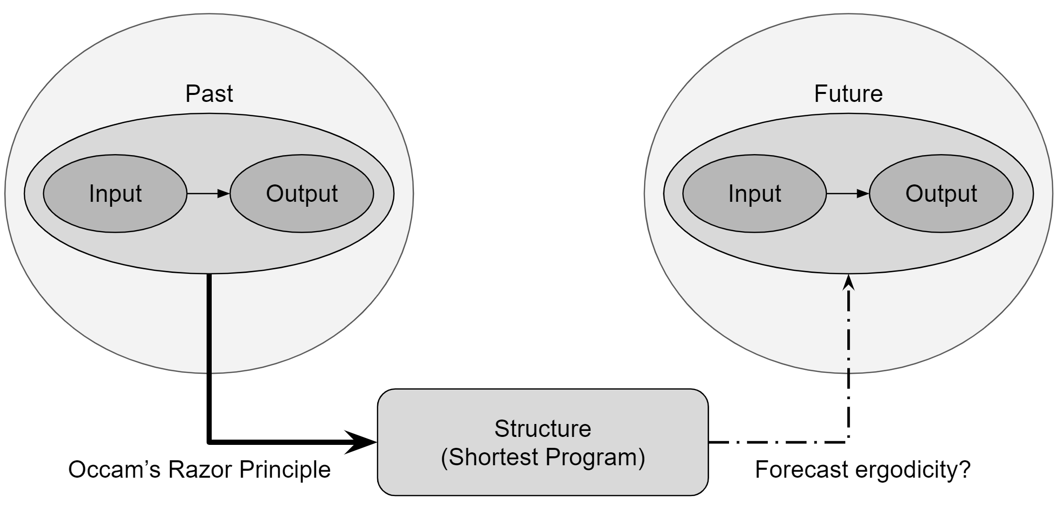
Figure 1: Illustration of problem reduction to inputs and outputs in forecasting.

II Background

For continuity a short introduction to KCS complexity is appropriate.

II-A KCS Complexity

KCS complexity considers a computer program $p$, a universal computer $\mathcal{U}$ and the corresponding computer output $x=\mathcal{U}(p)$. Let the length of program $p$, in bits, be $\ell(p)$. There are many programs that can generate a given output $x$. The KCS complexity, $K(x)$, is the length of the shortest binary program $p$ that generates the object $x$ [12, 13, 20, 21]:

$$K_{\mathcal{U}}(x)=\min_{p}\left\{\ell(p):\mathcal{U}(p)=x\right\}.$$ (1)

When additional information $y$ is provided as an input to the universal computer $\mathcal{U}$ along with the program $p$ to generate the binary string $x$, the conditional KCS complexity is defined as:

$$K_{\mathcal{U}}(x|y)=\min_{p}\left\{\ell(p):\mathcal{U}(p,y)=x\right\}.$$ (2)

For every program $p$, for a universal computer $\mathcal{U}$, the program $p$ can be translated to any other universal computer $\mathcal{A}$. The maximum cost of the translation is the constant $c$ equal to the length of the shortest program that translates from $\mathcal{U}$ to $\mathcal{A}$ [12]. So, for any pair of universal computers $\mathcal{U}$ and $\mathcal{A}$

$$K_{\mathcal{U}}(x)\leq K_{\mathcal{A}}(x)+c.$$

The constant $c$ does not depend on $p$. So it is possible to use any universal computer $\mathcal{U}$ as a fixed reference to measure the algorithmic complexity by adding the constant. More generally,

$$\mid K_{\mathcal{U}}(x)-K_{\mathcal{A}}(x)\mid\leq c$$ (3)

where the constant $c$ is independent of $p$. The bound in (3) can be written more simply as

$$K_{\mathcal{U}}(x)\underset{\overset{c}{}}{=}K_{\mathcal{A}}(x).$$

This equality allows us to drop reference to the specific computer $\mathcal{U}$ in future discussions about KCS complexity.

Example 1.

Consider the program that prints a concatenation $x$ of the binary numbers from 0 to $n$ (e.g. the binary Champernowne sequence [22, 23] for the first $n+1$ non negative integers):

PROGRAM 1:print(’011011100101110111100010011010101111001101111011111000010001100101001110100...’)Another program that prints the same binary string $x$ is:

PROGRAM 2:for i in range(n+1):  print(’{0:b}’.format(i), end=’’)The length of program 1 grows as $O\left(n\log n\right)$, while the length of program 2 grows as $O(\log n)$. So, for large $n$, program 2 is always shorter than program 1. where $\log n$ relates to the length of the bit stream in the second program.

From this example, given a concatenation $x$ of binary numbers from 0 to $n$, the KCS complexity of $x$ is bounded by

$$K\left(x\mid\ell(p)\right)\leq\log n+c$$

III Forecastability

This section contains the core definitions on algorithmic information forecastability and some related analysis illustrated with simple examples. More detailed examples are presented in Section V.

The data from the past is the training data. Both the past data and the future data include inputs and outputs. In the definitions, the available data includes the past data and some inputs of the future data. The predictions are the outputs of the future.

Let $\mathcal{F}$ be the countable set of all finite binary strings. Let $\accentset{\rightharpoonup}{X}_{M}$ be a $M$ vector such that each of its components belongs to $\mathcal{F}$, where $M\in\mathbb{N}\cup\{\infty\}$. For $N\leq M$, let $\accentset{\rightharpoonup}{X}_{N}$ be the first $N$ components of input data $\accentset{\rightharpoonup}{X}_{M}$. Define analogously the output data $\accentset{\rightharpoonup}{Y}_{M}$ and $\accentset{\rightharpoonup}{Y}_{N}$. The length of $x_{m}\in\accentset{\rightharpoonup}{X}_{M}$ can be different than the length of $y_{m}\in\accentset{\rightharpoonup}{Y}_{M}$. Table I outlines these elements.

The pair $\left(\accentset{\rightharpoonup}{X}_{N},\accentset{\rightharpoonup}{Y}_{N}\right)$ represents the training data, which can be viewed as occuring in the past. The goal of any machine intelligence application is to forecast the future outputs $\accentset{\rightharpoonup}{Y}_{M}\setminus\accentset{\rightharpoonup}{Y}_{N}=\left\{y_{N+1},y_{N+2},\dots,y_{M}\right\}$ given $\left(\accentset{\rightharpoonup}{X}_{M},\accentset{\rightharpoonup}{Y}_{N}\right)$, where for two sets $A$ and $B$, $A\setminus B=A\overline{B}$ is the set difference between $A$ and $B$.

TABLE I: Outline of training and future.

	Past (Training Data)	Future
Input	$\accentset{\rightharpoonup}{X}_{N}$	$\accentset{\rightharpoonup}{X}_{M}\setminus\accentset{\rightharpoonup}{X}_{N}$
$\accentset{\rightharpoonup}{X}_{M}$	$x_{1},\dots,x_{N}$	$x_{N+1},\dots,x_{M}$
Output	$\accentset{\rightharpoonup}{Y}_{N}$	$\accentset{\rightharpoonup}{Y}_{M}\setminus\accentset{\rightharpoonup}{Y}_{N}$
$\accentset{\rightharpoonup}{Y}_{M}$	$y_{1},\dots,y_{N}$	$y_{N+1},\dots,y_{M}$

III-A Oracle Forecastability

We first look at the case where predictions are always exact. That is, given the training data and the future input, the future output is perfectly predicted. This is achieved by means of the structure of the training data. We call these predictions to be oracle forecastable, because the shortest program that compresses the training data can be applied to the future input and print the future output with perfect precision, working as a flawless oracle. In the general case, the structure of the training data will compress the data from the past in a way that will include subroutines for the different classes of inputs. Within each class, the relation between input and output is the same, so, the structure compresses that class with a subroutine that implements the relation with an identification of the set of inputs that the relation applies to.

Definition 1.

The pair of vectors $\left(\accentset{\rightharpoonup}{X}_{M},\accentset{\rightharpoonup}{Y}_{M}\right)$ is oracle forecastable (OF) for $N$ if, for all $m\in\{N,\dots,M\}$,

$$K\left(y_{m}\middle|\accentset{\rightharpoonup}{X}_{N},\accentset{\rightharpoonup}{Y}_{N},x_{m}\right)\underset{\overset{c}{}}{=}0.$$ (4)

The equality in (4), as in subsequent definitions, is up to a constant. Here, this constant is the length of the forecasting program responsible of doing the prediction. The forecasting program pipes the future input to the subroutine that implements the structure from the training data and prints the output.

The pair $\left(\accentset{\rightharpoonup}{X}_{M},\accentset{\rightharpoonup}{Y}_{M}\right)$ is trivially OF for $N=M$.

According to Definition 1, OF for $N$ requires the conditional KCS complexity of every future ($m>N$) output, given the future input and the training data, to be 0. Therefore, under OF perfect accuracy is achieved.

Remark 1.

OF does not suggest how to obtain perfect accuracy.

Here are two elaborations.

1. For $N^{\prime}\in\{N+1,\dots,M\}$, let $\accentset{\rightharpoonup}{X}_{N^{\prime}}=\left(\accentset{\rightharpoonup}{X}_{N},x_{N+1},\cdots,x_{N^{\prime}}\right)$. A particular case of an OF for $N$ sequence is

   $$K\left(y_{N^{\prime}}\middle|\accentset{\rightharpoonup}{Y}_{N},\accentset{\rightharpoonup}{X}_{N^{\prime}}\right)\underset{\overset{c}{}}{=}0.$$ (5)

   Thus, the future input in (4) is made only of $x_{m}$, whereas, in (5) the future input includes $x_{N+1},x_{N+2},\ldots,x_{N^{\prime}}$. To present this particular case more clearly, we can go from (5) to (4):

   $$K\left(y_{N^{\prime}}\middle|\accentset{\rightharpoonup}{Y}_{N},\accentset{\rightharpoonup}{X}_{N^{\prime}}\right) =K\left(y_{N^{\prime}}\middle|\accentset{\rightharpoonup}{Y}_{N},\accentset{\rightharpoonup}{X}_{N},x_{N+1},\dots,x_{N^{\prime}}\right)$$

   $$=K\left(y_{N^{\prime}}\middle|\accentset{\rightharpoonup}{X}_{N},\accentset{\rightharpoonup}{Y}_{N},x_{N^{\prime}}^{*}\right),$$

   where $x_{N^{\prime}}^{*}=\left(x_{N+1},\dots,x_{N^{\prime}}\right)$. That is, the vector of inputs between $N+1$ and $N^{\prime}$ can be considered as the future input in (4). This addresses the fact that algorithms that change over time are included in Definition 1. Algorithmic information forecastability thus applies to both static algorithms and algorithms that change over time.

2. By Definition 1,

   $$\text{OF}\text{ for }N\Rightarrow K\left(\accentset{\rightharpoonup}{Y}_{M}\middle|\accentset{\rightharpoonup}{Y}_{N},\accentset{\rightharpoonup}{X}_{M}\right)\underset{\overset{c}{}}{=}0.$$ (6)

   The converse is true for some $\mathcal{M}\in\{N,\dots,M-1\}$:

   $$\text{OF for some }\mathcal{M}\Leftarrow K\left(\accentset{\rightharpoonup}{Y}_{M}\middle|\accentset{\rightharpoonup}{Y}_{N},\accentset{\rightharpoonup}{X}_{M}\right)\underset{\overset{c}{}}{=}0.$$ (7)

   However, depending on the pair of vectors $\left(\accentset{\rightharpoonup}{X}_{M},\accentset{\rightharpoonup}{Y}_{M}\right)$ being finite or infinite the significance of the implication in (7) is different.

   Lemma 1.

   For $\left(\accentset{\rightharpoonup}{X}_{M},\accentset{\rightharpoonup}{Y}_{M}\right)$ finite and $N<M$, if $K\left(\accentset{\rightharpoonup}{Y}_{M}\middle|\accentset{\rightharpoonup}{Y}_{N},\accentset{\rightharpoonup}{X}_{M}\right)\underset{\overset{c}{}}{=}0$, then $\left(\accentset{\rightharpoonup}{X}_{M},\accentset{\rightharpoonup}{Y}_{M}\right)$ is OFE at least for $N=M-1$.

   Proof.

   The vector $\accentset{\rightharpoonup}{X}_{M}$ might contain information which is not in $\accentset{\rightharpoonup}{X}_{N}$ when $N<M$. But if $N=M-1$, then $\accentset{\rightharpoonup}{X}_{M}\setminus\accentset{\rightharpoonup}{X}_{N}=x_{N+1}=x_{M}$, which corresponds to the input $x_{m}$ in Definition 1. In this case the information only comes from one element that satisfies the definition of OF. ∎

   Example 2.

   Electric load forecasting consist of predicting the demand for electricity based on historical data and other inputs such as weather forecast. Electric load forecasting is not OF for $N<M$ because the output cannot be forecast exactly [24]. If data is collected on a daily basis, the forecasting inputs can include at most the electric load of the previous day. Therefore, were the input of tomorrow available, the forecasting of today would be trivial. Alas, the input of tomorrow is not available today. Additionally, this example illustrates that $\left(\accentset{\rightharpoonup}{X}_{M},\accentset{\rightharpoonup}{Y}_{M}\right)$ is not OF for any $N<M$ when the output is random, according to Definition 1.

   The next lemma says that if the conditional Kolmogorov complexity of the output given the input and the training data goes to zero as $M\rightarrow\infty$, then the limit is actually hit for some finite $\mathcal{M}$. The implication is that under this condition, the pair $\left(\accentset{\rightharpoonup}{X}_{M},\accentset{\rightharpoonup}{Y}_{M}\right)$ is OF for all $m>\mathcal{M}$.

   Lemma 2.

   If

   $$\lim_{M\rightarrow\infty}K\left(\accentset{\rightharpoonup}{Y}_{M}\middle|\accentset{\rightharpoonup}{Y}_{N},\accentset{\rightharpoonup}{X}_{M}\right)\underset{\overset{c}{}}{=}0,$$ (8)

   then there exists $\mathcal{M}$ such that for all $m>\mathcal{M}$,

   $$K\left(y_{m}\middle|\accentset{\rightharpoonup}{Y}_{N},\accentset{\rightharpoonup}{X}_{m}\right)\underset{\overset{c}{}}{=}0.$$

   Proof.

   Assume that for all $\mathcal{M}$ there is an $m>\mathcal{M}$ such that $K\left(y_{m}\middle|\accentset{\rightharpoonup}{Y}_{N},\accentset{\rightharpoonup}{X}_{m}\right)$ is not zero. Since Kolmogorov complexity is always a non-negative integer, this implies that $\lim_{M\rightarrow\infty}K\left(\accentset{\rightharpoonup}{Y}_{M}\middle|\accentset{\rightharpoonup}{Y}_{N},\accentset{\rightharpoonup}{X}_{M}\right)\underset{\overset{c}{}}{\geq}1$, which contradicts (8). ∎

   Corollary 2.1.

   Choose $\mathcal{M}$ as introduced in Lemma 2 and substitute $\accentset{\rightharpoonup}{Y}_{N}$ by $\accentset{\rightharpoonup}{Y}_{\mathcal{M}}=\{\accentset{\rightharpoonup}{Y}_{N},y_{N+1},\dots,y_{\mathcal{M}}\}$, then there exists $\mathcal{M}$ such that for all $m>\mathcal{M}$,

   $$K\left(y_{m}\middle|\accentset{\rightharpoonup}{Y}_{\mathcal{M}},\accentset{\rightharpoonup}{X}_{m}\right)\underset{\overset{c}{}}{=}0$$

   which is equivalent to the particular case of OF for $\mathcal{M}$ in (5).

The next two lemmas address some applications to Markov chains.

Lemma 3.

Let $\left\{\accentset{\rightharpoonup}{X}_{M}\right\}$ be an absorbing Markov chain with state space $\Omega$. Let

$$f:\Omega \to\mathcal{F}$$

$$x_{m} \mapsto y_{m}.$$

Then the pair $\left(\accentset{\rightharpoonup}{X}_{M},\accentset{\rightharpoonup}{Y}_{M}\right)$ is OF for some finite $N$.

Proof.

In an absorbing Markov chain, after being in any of the states of the chain, an absorbing state is reached in a finite number of steps. As $M\rightarrow\infty$, an absorbing state will be reached at some time almost surely. Let $a$ be the first time an absorbing state is reached. Then for all $m\geq a$, $x_{m}=x_{a}$ and $y_{m}=y_{a}$, and the result follows. ∎

Lemma 4.

Let $\left\{\accentset{\rightharpoonup}{X}_{M}\right\}$ be an irreducible finite Markov chain with state space $\Omega$. Let

$$f:\Omega \to\mathcal{F}$$

$$x_{m} \mapsto y_{m}.$$

Then the pair $\left(\accentset{\rightharpoonup}{X}_{M},\accentset{\rightharpoonup}{Y}_{M}\right)$ is OF for some finite $N$.

Proof.

An irreducible finite Markov chain is also recurrent, that is, every state will appear in $\left\{\accentset{\rightharpoonup}{X}_{M}\right\}$ infinitely often. Choosing $N$ large enough, the training data will include every possible input and output of $f$ arbitrarily many times, and the result follows. ∎

III-B Precise Forcastability

Precision is defined for each application. For example, by an absolute error distance, by a percentage, by a Hamming distance, or by design constraints. Notice that, in general, an output is precise if it is in a predefined set of possible outcomes. To formally encompass every possible precision constraint, the following formulation is used.

Let $B(y_{m},\epsilon_{m})=\left\{y^{*}_{m}:d(y_{m},y^{*}_{m})<\epsilon_{m}\right\}$ be a ball with center $y_{m}$ and radius $\epsilon_{m}$ under certain metric $d$, defining the precision.

Definition 2.

The pair $\left(\accentset{\rightharpoonup}{X}_{M},\accentset{\rightharpoonup}{Y}_{M}\right)$ is precise forecastable (PF) up to $\epsilon$ for $N$, if, for all $m\in\{N,\dots,M\}$, there exists $y^{*}_{m}\in B(y_{m},\epsilon_{m})$ such that

$$K\left(y^{*}_{m}\middle|\accentset{\rightharpoonup}{X}_{N},\accentset{\rightharpoonup}{Y}_{N},x_{m}\right)\underset{\overset{c}{}}{=}0,$$ (9)

where $\epsilon=[\epsilon_{1},\ldots,\epsilon_{M}]$ is the level of precision.

The meaning underlying this definition is parallel to the previous case of OF. We are using the structure that is already present in the training data and in the current input to determine the desired output. And this is achieved by means of the algorithmic information of the available data, so that the Kolmogorov complexity of the output, given the available data, is zero. The only thing that changes in the definition of PF is that we introduce a tolerance for the precision of the forecast.

We have formalized the precision in the broadest possible way for PF to be applicable in the general case. More particularly, the following lemma elaborates on one of the most common and intuitive conceptions of precision, that is, when the error is bounded by the absolute value distance. In this case, there is a relation between the magnitude of the absolute value error and the KCS complexity of the error but this relation is not one of equivalence.

Lemma 5.

For the ball

$$B(y_{m},\epsilon_{m})=\left\{y^{*}_{m}:\left|y_{m}-y^{*}_{m}\right|<\epsilon_{m}\right\},$$ (10)

PF implies

$$K\left(y_{m}\middle|\accentset{\rightharpoonup}{X}_{N},\accentset{\rightharpoonup}{Y}_{N},x_{m}\right)\leq C_{\epsilon},$$ (11)

for all $m\in\{N,\dots,M\}$, where $C_{\epsilon}$ is a constant that bounds the KCS complexity of the error.

Proof.

We have

$$K\left(y_{m}\middle|\accentset{\rightharpoonup}{X}_{N},\accentset{\rightharpoonup}{Y}_{N},x_{m}\right)\underset{\overset{c}{}}{=}K\left(y_{m}\middle|y_{m}^{*}\right)\underset{\overset{c}{}}{\leq}C_{\epsilon},$$ (12)

where equality is up to a constant that accounts for the difference between the length of the forecasting program in $K\left(y_{m}\middle|\accentset{\rightharpoonup}{X}_{N},\accentset{\rightharpoonup}{Y}_{N},x_{m}\right)$ and the length of the program that performs an arithmetic operation in $K\left(y_{m}\middle|y_{m}^{*}\right)$. The latter also accounts for a constant in the inequality. Let

$$C_{\epsilon}=\max_{m\in[N,\dots,M]}K\left(y_{m}\middle|y_{m}^{*}\right)\underset{\overset{c}{}}{\leq}\lg^{*}(\epsilon_{m})$$ (13)

where $\lg^{*}(\epsilon_{m})$ is the length of a self-delimiting encoding of the $\epsilon_{m}$ in bits (see Appendix VI). The inequality is up to a constant that includes the sign or direction of $y_{m}-y_{m}^{*}$. ∎

The previous lemma shows that, for the ball in (10), if the error is bounded, then the KCS complexity of the error is bounded as well. However, the converse is not true. To explain it, there are instances of low KCS complexity, such as the instruction in pseudocode “flip_all_bits”, that can be short enough to satisfy (11) while not fitting the definition of PFE. In general, a bound for the KCS complexity of the error does not bound the error itself.

In a different example, the precision can consist of a Hamming distance bound, where the Hamming distance is defined as

$$H\left(y,y^{*}\right)=\sum_{i=1}^{\ell}\left[y_{i}\neq y_{i}^{*}\right]$$

for two binary strings $y=(y_{1},\dots,y_{\ell}),y^{*}=(y_{1}^{*},\dots,y_{\ell}^{*})$. Consider, for instance, images with black and white pixels, for which black pixels take the binary value of 0 and white pixels take value 1. Images are visualized in 2 dimensions, but they can be converted to one dimensional arrays for the theoretical analysis. Then

$$B(y_{m},\epsilon_{m})=\left\{y^{*}_{m}:\text{H}\left(y_{m},y^{*}_{m}\right)\leq h\right\}$$ (14)

where $h$ is the bound for the precision.

In another example, the distance $d$ can also be a Boolean attribute. For instance, assessing if a solution satisfies a series of engineering requirements, with margin to favor selected conflicting goals.

The previous examples illustrate the general formulation of PF and its applicability to different metrics. Note the relation between OF and PF:

Remark 2.

OF for $N$, in (4), is a particular case of PF for $N$, in (9), where the precision is maximally constrained with $B(y_{m},\epsilon_{m})=\left\{y_{m}\right\}$ for all $m$.

So, it follows that OF is a subset of PF, as every pair $\left(\accentset{\rightharpoonup}{X}_{M},\accentset{\rightharpoonup}{Y}_{M}\right)$ that is OF for $N$ is also PF for $N$.

III-C Probabilistic Forecastability

Probabilistic forecastability applies when a subset of elements in a pair $\left(\accentset{\rightharpoonup}{X}_{M},\accentset{\rightharpoonup}{Y}_{M}\right)$ is PF. In plain language this means that there is certain probability that the predictions will be precise, which is formalized in the following definition.

Definition 3.

The pair $\left(\accentset{\rightharpoonup}{X}_{M},\accentset{\rightharpoonup}{Y}_{M}\right)$ is probabilistic forecastable (PrF) for $N$, if for a fraction $P$ of the elements $\left(x_{m},y_{m}\right)$, $m\in\{N,\dots,M\}$, there exists $y^{*}_{m}\in B(y_{m},\epsilon_{m})$ such that

$$K\left(y^{*}_{m}\middle|\accentset{\rightharpoonup}{X}_{N},\accentset{\rightharpoonup}{Y}_{N},x_{m}\right)\underset{\overset{c}{}}{=}0.$$ (15)

This definition follows the same logic as in OF and PF. That is, given the structure of the available data, the prediction does not need any additional algorithmic information (this is why the expression equals zero in (15)). Everything that is needed is a program that identifies the class of the current input, locates the subroutine for that class in the structure, and obtains the corresponding output (the length of this program is included in the constant $c$ under the equal sign in (15)). What differentiates PrF for $N$ from PF for $N$ is that the probability of achieving precision is not necessarily 1.

The pair $\left(\accentset{\rightharpoonup}{X}_{M},\accentset{\rightharpoonup}{Y}_{M}\right)$ is trivially PrF for $P=0$.

PrF is broad enough to encompass any amount of algorithmic information from the available data with capacity to forecast some future data. The probability $P$ accounts for the ratio of the future elements $\accentset{\rightharpoonup}{Y}_{M}\setminus\accentset{\rightharpoonup}{Y}_{N}$ that are forecastable to a given degree of precision.

Depending on the problem, only one bit of information or larger amounts of information can be necessary. To visualize it with a simple example, a bride and bridegroom may only need one bit of information to know if it is going to rain or not on the day of their wedding to decide if they celebrate it indoors or outdoors. Instead, a farmer needs more information about the amount of rain. One bit can still be significant for him, but he would need at least 3 categories: (a) not enough rain, (b) just the right amount of rain and (c) too much rain; that is more than one bit of information. The farmer needs more details about the rain than the couple. And the farmer needs that information for each day of the year with high probability that the precipitation will fit the forecast. However, in the case of the wedding, they only need one bit of information, but they would need it more accurately if possible.

Regarding the amount of forecastable elements that non-trivial PrF requires:

• When $\left(\accentset{\rightharpoonup}{X}_{M},\accentset{\rightharpoonup}{Y}_{M}\right)$ is finite, PrF for $N$ only requires some $y_{m}$, $m\in\{N,\dots,M\}$, to be forecastable at a particular precision. Even if there is only one forecastable pair $\left(x_{m},y_{m}\right)$, that is sufficient to make $P>0$

• When $\left(\accentset{\rightharpoonup}{X}_{M},\accentset{\rightharpoonup}{Y}_{M}\right)$ is infinite, non-trivial PrF for $N$ requires a fraction $P>0$ of the elements $y_{m}$ from $\accentset{\rightharpoonup}{Y}_{M}\setminus\accentset{\rightharpoonup}{Y}_{N}$ to be forecastable at a particular precision. No matter how small the fraction $P$ is, the amount of such forecastable elements must be infinite. Otherwise, a finite amount of elements in an infinite series is negligible, given that no information about their location within the series is provided. If their location was known, it would be possible to truncate an infinite $\left(\accentset{\rightharpoonup}{X}_{M},\accentset{\rightharpoonup}{Y}_{M}\right)$ pair into a finite one

Remark 3.

PF is a particular case of PrF where $P=1$.

The previous remark shows that PF is a subset of PrF, as every pair $\left(\accentset{\rightharpoonup}{X}_{M},\accentset{\rightharpoonup}{Y}_{M}\right)$ that is PF for $N$ is also PrF for $N$ with $P=1$. The conditions for PrF and PF (Definition 3 and 2, respectively) are similar, but while PrF only requires a fraction $P$ of the elements in $\accentset{\rightharpoonup}{Y}_{M}\setminus\accentset{\rightharpoonup}{Y}_{N}$ to satisfy those conditions, PF requires all elements in $\accentset{\rightharpoonup}{Y}_{M}\setminus\accentset{\rightharpoonup}{Y}_{N}$ to satisfy those conditions.

III-D Forecast Ergodicity

In this section we propose the concept forecast ergodicity as a measure of the ability to forecast future events from data in the past. We model this bound by the algorithmic complexity of the available data.

Definition 4.

The forecast ergodicity (FE), $\mathcal{E}\left(\accentset{\rightharpoonup}{X}_{M},\accentset{\rightharpoonup}{Y}_{M}\right)$, of a pair $\left(\accentset{\rightharpoonup}{X}_{M},\accentset{\rightharpoonup}{Y}_{M}\right)$ is defined as a measure of the algorithmic information in the training data that is useful to forecast the future. The FE is bounded by:

$$\mathcal{E}\left(\accentset{\rightharpoonup}{X}_{M},\accentset{\rightharpoonup}{Y}_{M}\right)\leq K\left(\accentset{\rightharpoonup}{Y}_{N}\middle|\accentset{\rightharpoonup}{X}_{N}\right).$$ (16)

Note that the inequality in (16) requires either all of the structure provided by the training data is needed to forecast the future, or a shorter program could do. That is, a part of the structure in the training data may not be necessary to forecast the future.

Let

• $\mathcal{E}_{\text{OF}}$ be the set of all OF pairs $\left(\accentset{\rightharpoonup}{X}_{M},\accentset{\rightharpoonup}{Y}_{M}\right)$ for $N$

• $\mathcal{E}_{\text{PF}}$ be the set of all PF pairs $\left(\accentset{\rightharpoonup}{X}_{M},\accentset{\rightharpoonup}{Y}_{M}\right)$ for $N$ and precision $\epsilon$

• $\mathcal{E}_{\text{PrF}}$ be the set of all PrF pairs $\left(\accentset{\rightharpoonup}{X}_{M},\accentset{\rightharpoonup}{Y}_{M}\right)$ for $N$ and precision $\epsilon$

Lemma 6.

For a given $N$ and precision $\epsilon$

$$\mathcal{E}_{\text{OF}}\subset\mathcal{E}_{\text{PF}}\subset\mathcal{E}_{\text{PrF}}$$ (17)

Proof.

The relation follows directly from remarks 2 and 3: OF is a particular case of PF with $B(y_{m},\epsilon_{m})=\left\{y_{m}\right\}$ for all $m\in\{N,\dots,M\}$, and PF is a particular case of PrF with $P=1$. ∎

IV Probabilistic Forecast Loci

Consider the case where the precision is as in (10). We can get a locus for the values of $P$ depending on $\epsilon$. An example, to be explained, is shown in Figure 2.

Definition 5.

The probabilistic forecast locus (PrF-locus) $\mathcal{L}$ of a pair $\left(\accentset{\rightharpoonup}{X}_{M},\accentset{\rightharpoonup}{Y}_{M}\right)$ is defined for a given $N$ as the image of the function

$$\mathcal{L}\left(\epsilon\right)=P_{\epsilon}$$ (18)

over the domain of $\epsilon$, where $P_{\epsilon}$ is the fraction of the predictions that are precise up to $\epsilon$.

When the PrF-locus is unknowable, experiments can generate a best effort approximation. In the next section, Example 3 analyzes the forecast ergodicity of a pseudo random number generator from a theoretical point of view. For that example, the experimental analysis did not achieve the theoretic optimum. For other problems, the theoretic optimum might not be known.

An example of the approximation of an PrF-locus is shown in Figure 2. It corresponds to the results of a particular machine intelligence that learns the pseudo random number generator [25] of Example 3, yet to be described.

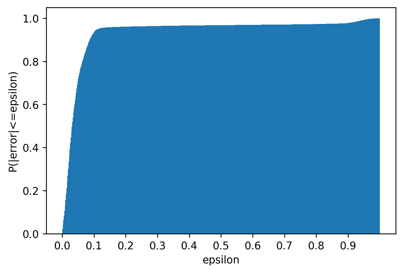
Figure 2: Experimental approximation of the PrF-locus $\mathcal{L}(\epsilon)$ of Example 3.

The plot shown in Figure 2 corresponds to the cumulative distribution function of the probability of the error having magnitude $\epsilon$. In this example, the prediction is always a number in the interval $[0,1)$ and the magnitude of the error is never greater than 1. The predictions were generated by a deep neural network trained with $1,000,000$ sequential pseudo random numbers. The graph was generated by measuring the error of the predictions of $100,000$ numbers equally distributed over the interval $[0,1)$ to approximate the PrFE-locus.

V Examples

Example 3.

Oracle forecastable (OF) Pseudo Random Number Generator (PRNG)

Consider this PRNG [25]

$$x_{n+1}=\text{frac}\left[\left(x_{n}+\pi\right)^{5}\right].$$ (19)

The PRNG works recursively after an initial seed $x_{0}$. The expression

$$y=\text{frac}\left[\left(x+\pi\right)^{5}\right]$$ (20)

is equivalent and it can operate either recursively or in combination with the use of different seeds. If $\accentset{\rightharpoonup}{X}_{M}$ is the vector of the successive inputs and $\accentset{\rightharpoonup}{Y}_{M}$ is the output, then the pair $\left(\accentset{\rightharpoonup}{X}_{M},\accentset{\rightharpoonup}{Y}_{M}\right)$ is oracle forecastable for some finite $N$. The mathematical formulation of the PRNG

$$f(x)=\text{frac}\left[\left(x+\pi\right)^{5}\right]$$ (21)

is helpful for the proof. Let $x_{0}$ be a seed for this PRNG and $x_{1},\dots,x_{N}$ the outputs of $N$ successive recursive iterations. Then:

$$K\left(\accentset{\rightharpoonup}{Y}_{N}\middle|\accentset{\rightharpoonup}{X}_{N}\right)\underset{\overset{c}{}}{\leq}\ell\left(p\right)+\lg^{*}\ell(p)$$ (22)

where $\accentset{\rightharpoonup}{X}_{N}=\left(x_{0},\dots,x_{N-1}\right)$, $\accentset{\rightharpoonup}{Y}_{N}=\left(y_{0},\dots,y_{N-1}\right)=\left(x_{1},\dots,x_{N}\right)$, $\ell(p)$ is the length of a program that implements the PRNG and $\lg^{*}\ell(p)$ is the length of a self-delimiting code that expresses $\ell(p)$ (see Appendix VI). This is trivially true for any value of $N$, but equality is needed for the proof. It is not possible to know the value of $N$ that produces

$$K\left(\accentset{\rightharpoonup}{Y}_{N}\middle|\accentset{\rightharpoonup}{X}_{N}\right)\underset{\overset{c}{}}{=}K(f)$$ (23)

where $f$ is the function in (21), but such $N$ exists and is finite.

Proof.

Following the same logic as in Lemma 2 and Corollary 2.1, given

$$\lim_{{M}\rightarrow\infty}K\left(\accentset{\rightharpoonup}{Y}_{{M}}\middle|\accentset{\rightharpoonup}{X}_{{M}}\right)\underset{\overset{c}{}}{=}K(f)$$ (24)

there exists $N$ such that

$$K\left(\accentset{\rightharpoonup}{Y}_{N}\middle|\accentset{\rightharpoonup}{X}_{N}\right)\underset{\overset{c}{}}{=}K(f).$$ (25)

Thus

$$\begin{split}K\left(y_{m}\middle|\accentset{\rightharpoonup}{X}_{N},\accentset{\rightharpoonup}{Y}_{N},x_{m}\right)&\underset{\overset{c}{}}{=}K\left(y_{m}\middle|\accentset{\rightharpoonup}{X}_{N},f,x_{m}\right)\\ &=K\left(y_{m}\middle|f,x_{m}\right)\\ &\underset{\overset{c}{}}{=}0\end{split}$$ (26)

for all $m>N$, satisfying the condition for OFE in (4). ∎

The forecast ergodicity of the PRNG is:

$$\begin{split}\mathcal{E}\left(\accentset{\rightharpoonup}{X}_{M},\accentset{\rightharpoonup}{Y}_{M}\right)&\leq K\left(\accentset{\rightharpoonup}{Y}_{N}\middle|\accentset{\rightharpoonup}{X}_{N}\right)\\ &\underset{\overset{c}{}}{=}K(f)\end{split}$$ (27)

Example 4.

Precise forecastable (PF) PRNG Web Service
Let the previous PRNG (Example 3) be running on a web server with a precision of $s$ bits. It provides numbers with a precision of at least $s^{\prime}<s$ bits. At any moment, the precision of the output is $s^{\prime\prime}\in\{s^{\prime},\dots,s\}$ bits. Let a sensor activated by radioactive decay trigger a change of precision, so the exact precision at a given time is unknown. If $\accentset{\rightharpoonup}{X}_{M}$ are the inputs to the PRNG on the server, with a precision of $s$ bits, and $\accentset{\rightharpoonup}{Y}_{M}$ are the outputs on the clients, with a precision of at least $s^{\prime}$ bits, then the pair $\left(\accentset{\rightharpoonup}{X}_{M},\accentset{\rightharpoonup}{Y}_{M}\right)$ is PF for $\epsilon=2^{s-s^{\prime}}$.

Regarding the analysis in (11), the KCS complexity of this noise can be bounded with $s-s^{\prime}$ bits plus the length of a self-encoding expression for $s-s^{\prime}$ (see Appendix VI),

$$C_{\epsilon}\leq s-s^{\prime}+\lg^{*}\left(s-s^{\prime}\right)+c.$$

up to a constant for the sign of $s-s^{\prime}$.

Example 5.

Probabilistic forecastable (PrF) Signal Spectrum Neural Network Classifier
Consider a neural network (NN) binary classifier trained to distinguish between LTE and Bluetooth signals. Bluetooth band (2400 to 2482.25 MHz) lies in between adjacent LTE bands, which are very close in the lower end and a little more separated on the upper end. Leakage between bands is very probable and other interferes, such as harmonics interference caused by the multiples of LTE frequencies in the Bluetooth band, can mess up the signals and make the classifier fail. In this context, the pair $\left(\accentset{\rightharpoonup}{X}_{M},\accentset{\rightharpoonup}{Y}_{M}\right)$ is, presumably, PrF, where the inputs are the signals and the outputs are the classifications. Let assume that the training data cover many typical cases that is possible to classify, while $1\%$ of the future signals are not represented by the training data. Then, the fraction $P$ of the future outputs that can be predicted to a certain precision could potentially be up to $99\%$. Experimentally, validation data serves to estimate $P$. Let the output $y_{m}\in[0,1]$ be within the interval $[0,0.25]$ for Bluetooth and $[0.75,1]$ for LTE, so we impose a precision of $\epsilon=0.25$. For an actual $P=0.99$, the experimental value will most probably be lower, for instance $P=0.95$, if $95\%$ of the validation data is correctly classified. The experimental value of $P$ is expected to be smaller than the theoretical one, but if the validation data is biased, the experimental $P$ can appear better. In any case, the validation set provides the best experimental approximation to the actual value.

Example 6.

PrF Reinforcement learning
A deep learning system that uses reinforcement learning updates the parameters, $\Theta$, of an artificial neural network model (agent) over time. At each iteration, $m$, the output of the agent is an action, $A_{m}$, and the inputs to the agent are the state of the environment, $S_{m}$, and a reward, $R_{m}$. The action can affect the state of the environment, which gives a reward to the agent. For this example, let

$$x_{m} =\left(\Theta_{m-1},S_{m},R_{m}\right),$$

$$y_{m} =\left(A_{m},\Theta_{m}\right).$$

The goal is to generate and maintain an agent whose actions optimize the return (aggregation of rewards). The reward can be absent or delayed and it can have a stochastic ingredient, so, the pair $\left(\accentset{\rightharpoonup}{X}_{M},\accentset{\rightharpoonup}{Y}_{M}\right)$ is PrF.

Sutton and Barto [26] note that most modern reinforcement learning uses finite Markov decision processes.

Example 7.

OF Finite Markov reinforcement learning
Adding some constrains to a reinforcement learning problem using a finite Markov decision process, we can obtain an OF problem. Consider the case where both the reward and the next state are a function of the action and the previous state, and the goal is to train an agent that chooses the action that optimizes the reward. This can apply to games such as checkers, chess, or go. These classes of games are OF for a finite $N$ [27].

The next example is an application of forecast ergodicity to dyadic numbers. Based on [28], let $T:(0,1]\rightarrow(0,1]$ be a mapping from the unit interval into itself defined by

$$T_{\omega}=\begin{cases}2\omega&\text{if }0<\omega\leq\frac{1}{2}\\ 2\omega-1&\text{if }\frac{1}{2}<\omega\leq 1.\end{cases}$$ (28)

Define also a Boolean function $d_{1}$ on $(0,1]$ by

$$d_{1}=\begin{cases}0&\text{if }0<\omega\leq\frac{1}{2}\\ 1&\text{if }\frac{1}{2}<\omega\leq 1,\end{cases}$$ (29)

and let $d_{i}(\omega)=d_{1}(T^{i-1}\omega)$. Then

Lemma 7.

$$\sum_{i=1}^{n}\frac{d_{i}(\omega)}{2^{i}}<\omega\leq\sum_{i=1}^{n}\frac{d_{i}(\omega)}{2^{i}}+\frac{1}{2^{n}},$$ (30)

for all $\omega\in(0,1]$ and $n\leq 1$.

Proof.

Easily proven by induction considering separate cases for $\omega\leq\frac{1}{2}$ and $\omega>\frac{1}{2}$ (see [28]). ∎

Every real number $\omega\in(0,1]$ can be arbitrarily approximated by dyadic numbers, which are always rational. In fact, for $\epsilon_{n}=2^{-n}$, each ball $B(\omega,\epsilon_{n})$ contains $\sum_{i+1}^{n}\frac{d_{i}(\omega)}{2^{i}}$, the dyadic approximation up to $n$ terms.

Example 8.

PF Dyadic approximation of real numbers
Every real number $\omega\in(0,1]$ can be arbitrarily approximated by dyadic numbers. Let each $x_{n}\in\left\{\accentset{\rightharpoonup}{X}_{\infty}\right\}$ be the dyadic expansion of $\omega$ with $n$ digits of precision, and for every $y_{n}\in\left\{\accentset{\rightharpoonup}{y}_{M}\right\},y_{n}=\sum_{i+1}^{n}\frac{d_{i}(\omega)}{2^{i}}$. For instance, if $\omega=0.01011$, then $x_{1}=0.0,x_{2}=0.01,x_{3}=0.010,x_{4}=0.0101,x_{5}=0.01011$, and $y_{1}=0,y_{2}=0.01,y_{3}=0.01,y_{4}=0.0101,y_{5}=0.01011$. For all $m\in\mathbb{N}$ define a precision $\epsilon_{m}=2^{-m}$ for the ball $B(\omega,\epsilon_{m})=\left\{\omega^{\prime}\in\mathbb{R}:\left|\omega-\omega^{\prime}\right|<\epsilon_{m}\right\}$. Then, for all $\epsilon>0$ there exists $N$ such that the output is precise forecastable.

VI Conclusion

Machine intelligence can accumulate data from the past to the present and do predictions within the boundaries of the algorithmic information forecastability of the data. Using algorithmic information theory, oracle, precise and probabilistic forecastability have been defined and illustrated through examples.

Forecastability is a property of the data and not the method used to perform the prediction. Not all data can be forecast, the most obvious of which is the repeated flipping of a fair coin. Forecastability does not necessarily mean the forecasting is straightforward or computationally inexpensive, e.g. forecasting the output of certain pseudo-random number generators. Design of forecasting algorithms remains a function of domain expertise about the data and computational power.

Marvin Minsky opined [1] “everybody should learn all about that [algorithmic information theory forecasting] and spend the rest of their lives working on it.” This paper is a step in application of algorithmic information processing to Minsky’s challenge.

[Recursive Self-Delimiting Code for the Function $\text{lg}^{*}$] To run a program $p$ in an universal computer $\mathcal{U}$, an indication of the length of the program has to be provided so it can halt when the end of the program is reached. And, in order to indicate the length of the program, the computer $\mathcal{U}$ needs to be informed about when to stop reading that number. Self-delimiting codes are used for this purpose.

For instance, 00 could encode the value 0 and 11 the value 1, while 01 would indicate the end of the number. The cost of this approach is twice the length of the number plus 2 bits for the ending: $2\log(n)+2$ bits.

A better approach, introduced in [12] and [13], consist of concatenating the length, with the length of the length, with the length of the length of the length, and so on, recursively, by adding the concatenations on the left, until the value 1 is reached. The self-encoding of the number $n$ would be something like this:

$$1\mathbin{\|}\dots\mathbin{\|}\log\left(\log\left(\log\left(n\right)\right)\right)\mathbin{\|}\log\left(\log\left(n\right)\right)\mathbin{\|}\log\left(n\right)\mathbin{\|}n\mathbin{\|}0$$

where $\mathbin{\|}$ is the symbol for the concatenation of two strings, and the 0 at the right indicates the end of the encoding.

In [13], when presenting this method, a previous knowledge of the depth of the recursion is assumed. However, adding some simple rules allows for a fully self-delimiting implementation without indication of the depth of the recursion. For example, the implementation we developed, based on this approach, encodes the number 1200 as

Ψ1111001011100101100000

with a length of 22 bits. It decomposes as

Ψ                     0 -> end
Ψ          10010110000  -> 1200 in binary
Ψ      1011             -> length of 1200
Ψ   100                 -> length of 11
Ψ 11                    -> length of 4
Ψ1                      -> start

which is written starting from the right (first 0, then the number, then the $\log$ of the number, then the $\log\log$ of the number, and so on), but it reads from bottom to top as in the next explanations

⬇

1 -> start (will read 2 next bits when

the code starts with a 1)

11 -> 3 in binary. Will read next 3 bits

(the binary length of 4 is 3):

ceil(log2(4+1)) = 3

100 -> 4 in binary. Will read next 4

bits(the binary length of 11

is 4): ceil(log2(11+1)) = 4

1011 -> 11 in binary. Will read

next 11 bits (the binary

length of 1200 is 11):

ceil(log2(1200+1)) = 11

10010110000 -> 1200 in binary

0 -> end

The encoding process goes from right to left. This implementation allows the computer to read the number and detect the end, with the rule of stopping when the next lecture starts by 0. With access to the decoding algorithm, no previous knowledge about the number or about the depth of the recursion is needed in order to decode it. The implementation used for this example encodes and decodes integers greater than or equal to 0 (the sign is provided independently). Even when some details are obviated from this explanation —details such as the special cases of the numbers 0 and 1 or the exceptions for the first iteration— the example provides a clear view of how the method works. For the decoding process, the reading starts from the left to the right as follows: after processing the first starting bit 1, then it reads $11_{2}=3$, so it now must proceed to read the next 3 bits, that is $100_{2}=4$, then it reads the next 4 bits, that is $1011_{2}=11$, it reads the next 11 bits, that is $10010110000_{2}=1200$, then, the next bit is 0, indicating the end of the encoding. So, the last number in the concatenation, 1200, is the self-delimited encoded number.

This self-delimiting encoding of the number 1200 has length 22; that is only a little shorter than the bit duplication method for this number, which requires $2\times 11+2=24$ bits. However, for larger numbers, the optimization becomes more clear, as shown in Figure 3.

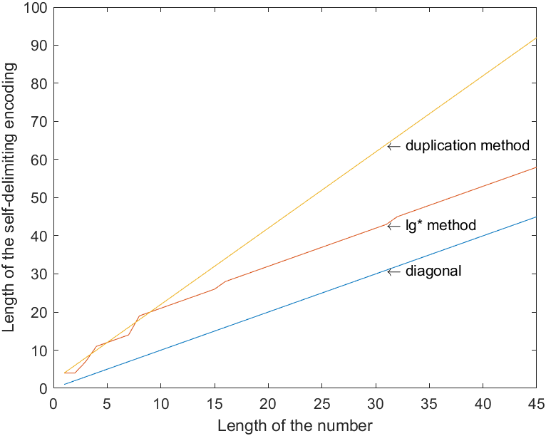
Figure 3: Length in bits of the self-delimiting encoding method of bit duplication and $\lg^{*}$ as a function of the length of the binary numbers. The difference between the bit duplication and the $\lg^{*}$ method is significant when the numbers are large.

Taking as reference the length of the number (diagonal line on Figure 3) the additional amount of bits required for bit duplication grows as $O(n)$, while with the $\lg^{*}$ method requires less bits for the representation.

References

- [1] G. Chaitin, R. Goldstein, M. Livio, and M. Minsky. (2014) The limits of understanding. World Science Festival. [Online]. Available: https://www.youtube.com/watch?v=DfY-DRsE86s
- [2] P. D. Grünwald, The minimum description length principle. MIT press, 2007.
- [3] G. Gilder, Gaming AI. Discovery Institute Press, 2020.
- [4] “Merriam webster dictionary on line,” https://www.merriam-webster.com/dictionary/ergodic.
- [5] L. Alaoglu and G. Birkhoff, “General ergodic theorems,” Proceedings of the National Academy of Sciences of the United States of America, vol. 25, no. 12, p. 628, 1939.
- [6] I. P. Cornfeld, S. V. Fomin, and Y. G. Sinai, Ergodic theory. Springer Science & Business Media, 2012, vol. 245.
- [7] A. Papoulis and S. U. Pillai, Probability, random variables, and stochastic processes. Tata McGraw-Hill Education, 2002.
- [8] D. Angluin, “Computational learning theory: survey and selected bibliography,” in Proceedings of the twenty-fourth annual ACM symposium on Theory of computing, 1992, pp. 351–369.
- [9] M. Anthony and N. Biggs, Computational learning theory. Cambridge University Press, 1997, vol. 30.
- [10] L. G. Valiant, “A theory of the learnable,” Communications of the ACM, vol. 27, no. 11, pp. 1134–1142, 1984.
- [11] ——, “Probably approximately correct: Nature’s algorithms for learning and prospering in a complex,” Communications of the ACM, vol. 27, no. 11, pp. 1134–1142, 1984.
- [12] T. M. Cover and J. A. Thomas, Elements of information theory (2. ed.). Wiley Interscience, 2006. [Online]. Available: http://www.elementsofinformationtheory.com/
- [13] M. Li and P. M. B. Vitányi, An Introduction to Kolmogorov Complexity and Its Applications, 4th Edition, ser. Texts in Computer Science. Springer, 2019. [Online]. Available: https://doi.org/10.1007/978-3-030-11298-1
- [14] R. J. Marks, W. A. Dembski, and W. Ewert, Introduction to Evolutionary Informatics. World Scientific, 2017.
- [15] K. Tadaki, “Algorithmic information theory,” in A Statistical Mechanical Interpretation of Algorithmic Information Theory. Springer, 2019, pp. 13–21.
- [16] R. Solomonoff, “A formal theory of inductive inference. part i,” Information and Control, vol. 7, no. 1, pp. 1–22, 1964. [Online]. Available: https://www.sciencedirect.com/science/article/pii/S0019995864902232
- [17] ——, “A formal theory of inductive inference. part ii,” Information and Control, vol. 7, no. 2, pp. 224–254, 1964. [Online]. Available: https://www.sciencedirect.com/science/article/pii/S0019995864901317
- [18] J. Rissanen, “Modeling by shortest data description,” Automatica, vol. 14, no. 5, pp. 465–471, 1978. [Online]. Available: https://www.sciencedirect.com/science/article/pii/0005109878900055
- [19] H. S. Bhat and N. Kumar, “On the derivation of the bayesian information criterion,” School of Natural Sciences, University of California, vol. 99, 2010.
- [20] W. Ewert, W. A. Dembski, and R. J. M. II, “Algorithmic specified complexity,” in Engineering and the Ultimate: An Interdisciplinary Investigation of Order and Design in Nature and Craft, J. Bartlett, D. Halsmer, and M. Hall, Eds. Blyth Institute Press, 03 2014, ch. 7, pp. 131–151.
- [21] N. K. Vereshchagin and P. M. B. Vitanyi, “Kolmogorov’s structure functions and model selection,” IEEE Transactions on Information Theory, vol. 50, no. 12, pp. 3265–3290, 2004.
- [22] C. S. Calude and K. Svozil, “Spurious, emergent laws in number worlds,” Philosophies, vol. 4, no. 2, p. 17, 2019.
- [23] D. G. Champernowne, “The construction of decimals normal in the scale of ten,” Journal of the London Mathematical Society, vol. 1, no. 4, pp. 254–260, 1933.
- [24] D. C. Park, M. A. El-Sharkawi, R. J. Marks, L. E. Atlas, and M. J. Damborg, “Electric load forecasting using an artificial neural network,” IEEE Transactions on Power Systems, vol. 6, no. 2, pp. 442–449, 1991.
- [25] G. Amigo, L. Dong, and R. J. Marks Ii, “Forecasting pseudo random numbers using deep learning,” in 2021 15th International Conference on Signal Processing and Communication Systems (ICSPCS), 2021, pp. 1–7.
- [26] R. S. Sutton and A. G. Barto, Reinforcement Learning: An Introduction, 2nd ed. The MIT Press, 2018. [Online]. Available: http://incompleteideas.net/book/the-book-2nd.html
- [27] J. Schaeffer, N. Burch, Y. Björnsson, A. Kishimoto, M. Müller, R. Lake, P. Lu, and S. Sutphen, “Checkers is solved,” Science, vol. 317, no. 5844, pp. 1518–1522, 2007. [Online]. Available: https://www.science.org/doi/abs/10.1126/science.1144079
- [28] P. Billingsley, Probability and Measure, ser. Wiley Series in Probability and Statistics. Wiley, 1995. [Online]. Available: https://books.google.com/books?id=z39jQgAACAAJ