Reinforcement Learning Approaches for Traffic Signal Control
under Missing Data

Abstract

The emergence of reinforcement learning (RL) methods in traffic signal control tasks has achieved better performance than conventional rule-based approaches. Most RL approaches require the observation of the environment for the agent to decide which action is optimal for a long-term reward. However, in real-world urban scenarios, missing observation of traffic states may frequently occur due to the lack of sensors, which makes existing RL methods inapplicable on road networks with missing observation. In this work, we aim to control the traffic signals in a real-world setting, where some of the intersections in the road network are not installed with sensors and thus with no direct observations around them. To the best of our knowledge, we are the first to use RL methods to tackle the traffic signal control problem in this real-world setting. Specifically, we propose two solutions: the first one imputes the traffic states to enable adaptive control, and the second one imputes both states and rewards to enable adaptive control and the training of RL agents. Through extensive experiments on both synthetic and real-world road network traffic, we reveal that our method outperforms conventional approaches and performs consistently with different missing rates. We also provide further investigations on how missing data influences the performance of our model.

1 Introduction

Traffic congestion has been a challenge in modern society and adversely affects economic growth, environmental sustainability, and people’s quality of life. For example, traffic congestion costs an estimated $\$87$ billion in lost productivity in the US alone Tirone (2022). Recently, reinforcement learning (RL) has shown superior performance over traditional transportation approaches in controlling traffic signals in dynamic traffic Arel et al. (2010); El-Tantawy et al. (2013); Oroojlooy et al. (2020); Wei et al. (2019a). The biggest advantage of RL is that it directly learns to take adaptive actions in response to dynamic traffic by observing the states and feedback from the environment after previous actions.

Although a number of literature has focused on improving RL methods’ performance in traffic signal control, RL cannot be directly deployed in the real world where accessible observations are sparse, i.e., some traffic states are missing Chen et al. (2019); Mai et al. (2019). In most cities where sensors are only installed at certain intersections, intersections without sensors cannot utilize RL and usually use pre-timed traffic signal plans that cannot adapt to dynamic traffic. Similar situations could happen when installed sensors are not properly functioning, which will lead to missing observations in the collected traffic states Duan et al. (2016) and the failure to deploy RL methods. Though there have been attempts such as using imitation learning to learn from the experience of human traffic engineers Li et al. (2020), these methods need manual design and cannot be easily extended to new scenarios. Thus the missing data issue still hinders not only the application of RL, but also the deployment of other adaptive control methods that require observing traffic states like MaxPressure Varaiya (2013).

In this paper, we investigate the traffic signal control problem under the real-world setting, where the traffic condition around certain intersections are never observed. To enable dynamic control over these intersections, we investigate how data imputation could help the control, especially how the imputation on state and reward can remedy the missing data challenge for RL methods. With imputed states, adaptive control methods from transportation could be utilized; with both imputed states and rewards, RL agents could be trained for unobserved intersections. Inspired by model-based RL, we also investigate to use the imaginary rollout with reward model for better performance. The main contributions of this work are summarized as follows:

$\bullet$ To the best of our knowledge, we are the first to adapt RL-based traffic signal control methods under the missing data scenario, hence improving reinforcement learning method’s applicability under more realistic settings. We test different kinds of approaches to control the intersections without observations. We propose a two-step approach that firstly imputes the states and rewards to enable the second step of RL training. The proposed approach can achieve better performance than only training RL agents at fully observed intersections or training RL agents on all intersections using only observed data without imputation, and also outperforms using pre-timed control methods.
$\bullet$ We investigate our methods under synthetic and real-world datasets with different missing rates and whether having neighboring unobserved intersections. The result shows our method is still effective in real-world scenarios. And the extensive studies on different missing rates and relationships of missing positions shows our methods perform better than pre-timed methods. We also extend our proposed methods for a highly heterogeneous dataset and justified their effectiveness, enhancing their applicability in real life.

2 Related Work

Traffic signal control methods. Optimizing traffic signal control to alleviate traffic congestion has been a challenge in the transportation field for a long time. Different approaches have been extensively studied, including rule-based methods Hunt et al. (1981); Sims and Dobinson (1980); Varaiya (2013) and RL-based methods Arel et al. (2010); Wei et al. (2019a, 2018) to optimize vehicle travel time or delay. Most of these studies, for example, IDQN method Wei et al. (2018), have significantly improved compared to pre-designed time control methods. However, to the best of our knowledge, there is no existing work on dealing with the unobserved intersections in dynamic traffic signal control methods.

Traffic data imputation. In real-world scenarios, full observation is not always accessible. An effective way to deal with the missing observations is data imputation, i.e., to infer the missing data to complete traffic observations. Earlier studies typically use historical data collected at each location to predict the values at missing positions of the same site Gan et al. (2015); Zhong et al. (2004). Recently, neural network-based methods have been proven effective and extended to be used in the traffic data imputation task Lv et al. (2015). These methods could be categorized into Recurrent Neural Networks (RNNs) Cui et al. (2020); Yao et al. (2018), Graph Neural Network (GNN) Wang et al. (2022) and Generative Adversarial Networks (GANs) Zhang et al. (2021). However, all the methods mentioned above also need the observation of all intersections to train models, while in reality, it is hard to fulfill. Store-and-forward method (SFM) Aboudolas et al. (2009) is another approach to model traffic state transition and is often used as the base model traffic simulation.

Model-based reinforcement learning. Model-based reinforcement learning (MBRL) methods utilize predictive models of the environment on the immediate reward or transition to provide imaginary samples for RL Luo et al. (2022). In MBRL with a reward model, an agent learns to predict the immediate reward of taking action at a certain state, and in this paper, we borrow this idea to train a reward model. In MBRL with a transition model, an agent usually has the direct observation of its own surrounding states, and a transition model is used to simulate the next states from current observations. Unlike MBRL with transition models, in this paper, some agents do not have observations of their own surroundings, where imputation methods are utilized to infer the current states (rather than next states) for those agents.

3 Preliminaries

In this section, we take the basic problem definition used in the multi-intersection traffic signal control Wei et al. (2019a) and extend it into the missing data scenario frequently encountered in the real world. An agent controls each intersection in the system. Given that only part of the agents can have their local observation of the total system condition as their state, we would like to proactively decide for all the intersections in the system which phases they should change to so as to minimize the average queue length on the lanes around the intersections. Specifically, the problem is characterized by the following major components $\braket{\mathcal{S},\mathcal{\hat{S}},\mathcal{A},\mathit{r},\Pi,\mathit{\gamma}}$:

$\bullet$ Observed state space $\mathcal{S}$ and imputed state space $\mathcal{\hat{S}}$. We assume that the system consists of a set of intersections $\mathcal{N}=\mathcal{N}_{o}\cup\mathcal{N}_{m}$, where $\mathcal{N}_{o}$ is the set of intersections where the agent can observe part of the system as its state $\mathit{s}\in\mathcal{S}$, and $\mathcal{N}_{m}$ is the set of intersections where the agent cannot observe the system. We follow setting from past works Wei et al. (2019b); Wu et al. (2021); Huang et al. (2021), and define $\mathit{s}_{t}^{j}$ for agent $j\in\mathcal{N}_{o}$ at time $t$, which consists of its current phase (which direction is in green light) and the number of vehicles on each lane at time $t$. Later we will introduce unobserved agent $k\in\mathcal{N}_{m}$, and how we can infer its state $\mathit{\hat{s}}_{t}^{k}\in\mathcal{\hat{S}}$ at time $t$.

$\bullet$ Set of actions $\mathcal{A}$. In the traffic signal control problem, at time $t$, an agent $i$ would choose an action $a_{t}^{i}$ from its candidate action set $\mathcal{A}_{i}$ as a decision for the next $\Delta t$ period of time. Here, we take acyclic control method, in which each intersection would choose a phase $p$ as its action $a_{t}^{i}$ from its pre-defined phase set, indicating that from time $t$ to $t+\Delta t$, this intersection would be in phase $p$.

$\bullet$ Reward $\mathit{r}$. Each agent $i$ obtains an immediate reward $\mathit{r}_{t}^{i}$ from the environment at time $t$ by a reward function $\mathcal{S}\times\mathcal{A}_{1}\times\dots\times\mathcal{A}_{N}\rightarrow\mathbb{R}$. In this paper, we want to minimize the travel time for all vehicles in the system, which is hard to optimize directly. Therefore, we define the reward for intersection $i$ as $\mathit{r}_{t}^{i}=-\Sigma_{l}u_{t}^{i,l}$ where $u_{t}^{i,l}$ is the queue length on the approaching lane $l$ at time t. Specifically, we denote $\mathit{r}_{t}^{j}$ as the observed reward for agent $j\in\mathcal{N}_{o}$ at time $t$, and the inferred reward $\mathit{\hat{r}}_{t}^{k}$ as the reward for agent $k\in\mathcal{N}_{m}$ at time $t$.

$\bullet$ Policy set $\Pi$ and discount factor $\mathit{\gamma}$. Intuitively, the joint actions have long-term effects on the system, so we want to minimize the expected queue length of each intersection in each episode. Specifically, at time $t$, each agent chooses an action following a certain policy $\mathit{\pi}:\mathcal{S}\rightarrow\mathcal{A}$.

An RL agent follows policy $\mathit{\pi}_{\theta}\in\Pi$ parameterized by $\theta$, aiming to maximize its total reward $G_{t}^{i}=\Sigma_{\tau=t}^{T}\mathit{\gamma}^{\tau-t}\mathit{r}_{t}^{i}$, where $T$ is total time steps of an episode and $\mathit{\gamma}\in[0,1]$ differentiates the rewards in terms of temporal proximity. Other rule-based agents are denoted as $\mathit{\pi}_{\varnothing}\in\Pi$.

Problem 1 (Traffic signal control under missing data).

Given a road network where only part of the intersections is observed with $\mathcal{S}$, the goal of this paper is to find a better $\Pi$, no matter whether it consists of $\mathit{\pi}_{\theta}$, $\mathit{\pi}_{\varnothing}$ or mixed policies of previous two kinds, that can minimize the average travel time of all vehicles.

In the RL framework, training and execution are two decoupled phases: (1) During execution, an agent takes actions based on its policy $\mathit{\pi}$ to roll out trajectories and evaluate their performances. For policies that take the current state as input, the agent can execute adaptive actions as long as the input states are available. For observed intersections $\mathcal{N}_{o}$, the input states could directly be observed state $\mathit{s}\in\mathcal{S}$; for unobserved intersections $\mathcal{N}_{m}$, the input states could be inferred $\mathit{\hat{s}}\in\mathcal{\hat{S}}$ using data imputation. (2) In the training phase, agents explore the environment, store experiences in the replay buffer, and update their policies to maximize their long-term rewards. The experiences usually consist of state $\mathit{s}_{t}$, reward $\mathit{r}_{t}$, action $a_{t}$, and next state $\mathit{s}_{t+1}$. Different from execution phase, which only requires the input states, the training phase of RL requires reward information. For unobserved intersections $\mathcal{N}_{m}$, the $\mathit{\hat{r}}_{t}$ could also be inferred with data imputation on the reward. Later in Sec. 4, we will introduce how the missing data in the training and execution phase would influence the design of methods to tackle the traffic signal control problem.

4 Methods under Missing Data

Figure 1: Overall framework of our proposed approaches. Red lines represent how the imputed data flows into unobserved intersections. And blue lines show how reward is imputed and used for imaginary rollout. In Remedy 1, we only impute states at $\mathcal{N}_{m}\$and enable agents at these intersections to take adaptive actions; In Remedy 2, we impute states and rewards together for training agents. (a) Remedy 1.1: RL agents at $\mathcal{N}_{o}\$take $s_{t}^{j},r_{t}^{j}$ for training their policies, and take $s_{t}^{j}$ during the execution phase. And MaxPressure agents at $\mathcal{N}_{m}\$take imputed $\hat{s}_{t}^{k}$ together with neighboring intersections’ $s_{t}^{j}$ during training and execution phases. (b) Remedy 1.2: RL agents take $s_{t}^{j},r_{t}^{j}$, and train based on these observable experiences. And at the $\mathcal{N}_{m}$, agents are transferred from $\mathcal{N}_{o}\$and take imputed $\hat{s}_{t}^{k}$ for taking actions during the execution phase. (c) Remedy 2.1: agents at $\mathcal{N}_{o}\$and $\mathcal{N}_{m}\$take $s_{t}^{j},r_{t}^{j}\text{ pairs or }\hat{s}_{t}^{k},\hat{r}_{t}^{k}$ pairs respectively and optimize their own policies during training. During execution, agents at $\mathcal{N}_{o}\$take $s_{t}^{j}$ from the environment, and agents at $\mathcal{N}_{m}\$take imputed $\hat{s}_{t}^{k}$ for execution. Different from Remedy 2.1, in (d) Remedy 2.2 and (e) Remedy 2.3, all agents share the same policy, while Remedy 2.3 has an additional imaginary rollout step.

Adaptive control methods like MaxPressure and RL-based methods dynamically adjust traffic signals based on real-time traffic state observations, which have been proven to work well on traffic signal control tasks. However, in the real-world scenario, these adaptive control methods cannot work properly at intersections $\mathcal{N}_{m}$ where real-time observations are missing. To adapt dynamic control methods to real-world, we explore the conventional approach and propose two effective imputation approaches to handle the failure of adaptive control at $\mathcal{N}_{m}$. The overall frameworks are shown in Figure 1.

4.1 Conventional Approaches

Under the missing data scenario, there are three direct approaches for traffic signal control: (1) pre-timed control, which sets fixed timings for all intersections; (2) the mixed control of RL and pre-timed agents, which uses RL agents only at observed intersections $\mathcal{N}_{o}$ and deploys pre-timed agents at unobserved intersections $\mathcal{N}_{m}$; (3) neighboring RL control, where agents at unobserved intersections $\mathcal{N}_{m}$ concatenate states from neighboring observed intersections as their own state and accumulate rewards from their neighboring observed intersections as their reward. This approach follows the general solution to the Partially Observable Markov Decision Process (POMDP) and assumes the traffic condition from observed neighboring intersections could reflect the unobserved traffic condition. This assumption might not hold when the number of missing intersections increases or the traffic is dynamic and complex.

4.2 Remedy 1: Imputation over Unobserved States

To enable $\mathcal{N}_{m}$ with dynamic control during execution, a natural solution is to impute unobserved states $\hat{s}_{t}^{k}$ at $\mathcal{N}_{m}\$for control methods. After the imputation of the states at unobserved intersections, dynamic control methods can be applied.

Imputation.

Since the state information at unobserved intersections is totally missing, it is inapplicable to train a model on data collected from unobserved intersections and recover unobserved states. Therefore, we need to pretrain a state imputation model that will be shared by all the unobserved intersections and apply it during the training of RL. Intuitively, vehicles currently on each lane are aggregated from its up-streaming connected lanes in the previous time step. Given the states of neighboring intersections $\mathcal{V}^{k}$ of intersection $k\in\mathcal{N}_{m}$, the state imputation at $k$ can be formally defined as follows:

$$\hat{s}_{t}^{k}=f(\mathcal{V}^{k}_{t-1})$$ (1)

where $f$ could be any state imputation model. In this paper, we investigate two pre-trained models, a rule-based Store-and-Forward model (SFM) and a neural network model. Their detailed descriptions can be found in Sec. 5.1.

Control.

After imputation, we investigate two control approaches that can function during execution.

$\bullet$ Approach 1: Adaptive control methods in transportation. Adaptive control methods in transportation usually require observation of the surrounding traffic conditions to decide the action for traffic signals. Without imputation, these methods cannot be applied directly. In this paper, following Wei et al. (2019a); Chen et al. (2020), we use one widely used adaptive control method, MaxPressure Varaiya (2013), to control traffic signals for unobserved intersections after imputation.

$\bullet$ Approach 2: Transferred RL models. Another method is to enable RL-based control at missing intersections by training an RL policy $\mathit{\pi}_{\theta}$ at observed intersections $\mathcal{N}_{o}\$and later transferring to $\mathcal{N}_{m}\$during execution. Since all agents share the same policy, we refer to this model-sharing agent as SDQN for later use. During execution, agent $j\in\mathcal{N}_{o}$ can directly use the states $s^{j}_{t}$ observed from the environment to take action $\mathit{\pi}_{\theta}(a^{j}_{t}|\mathit{s}^{j}_{t})$. For agent $k\in\mathcal{N}_{m}$, it first imputes states $\mathit{\hat{s}}^{k}_{t}$ and then takes action $\mathit{\pi}_{\theta}(a^{k}_{t}|\mathit{\hat{s}}^{k}_{t})$ based on the imputed states $\mathit{\hat{s}}^{k}_{t}$. In this solution, we use $(s^{j}_{t},r^{j}_{t},a^{j}_{t},s^{j}_{t+1})$ from all the observed intersections $j\in\mathcal{N}_{o}$ as experiences to train an RL model shared by all intersections. This approach can significantly improve sample efficiency, and all training samples can reflect the true state of the environment. However, since the agent is only trained on the experiences from observed intersections $\mathcal{N}_{o}$, it might not be able to cope with unexplored situations at $\mathcal{N}_{m}$, which could result in a loss of generality based on the agent’s policy.

4.3 Remedy 2: Imputation over Unobserved States and Rewards

To enable agents to learn from experiences on unobserved intersections $\mathcal{N}_{m}$, it is necessary to impute both state and reward for unobserved intersections $k\in\mathcal{N}_{m}$. After getting both the imputed state $\mathit{\hat{s}}_{t}^{k}$ and inferred reward $\hat{r}_{t}^{k}$ at $\mathcal{N}_{m}$, we can train agents with these imputed experiences $(\mathit{\hat{s}}_{t}^{k},\hat{r}_{t}^{k},a_{t}^{k},\mathit{\hat{s}}_{t+1}^{k})$.

Imputation.

The process of state imputation is the same as described in Sec. 4.2. For reward imputation, we use a neural network to infer $\mathit{\hat{r}}_{t}^{k}$ for $\mathcal{N}_{m}$ with state and action as input and pre-train it before RL training starts. In the pre-training phase, we first run with a conventional control approach to collect $(s^{j}_{t},r^{j}_{t},a^{j}_{t})$ as training samples from observed intersections $j\in\mathcal{N}_{o}$, upon which we train the reward imputation model $g_{\psi}$ with MSE Loss:

$$\begin{split}&\mathcal{L}(\psi)=\frac{1}{n}\sum_{n}{(g_{\psi}(s^{j},a^{j})-r^{j})^{2}}\end{split}$$ (2)

During the RL training phase, the original $s_{t}^{j}$ at $\mathcal{N}_{o}\$returned from the environment will first pass through state imputation model and get the recovered data $\hat{s}^{k}_{t}$ at $\mathcal{N}_{m}\$. The imputed $\hat{s}_{t}^{k}$ combining $a_{t}^{k}$ will be fed into $g_{\psi}$ which could be described as:

$$\hat{r}^{k}_{t}=g_{\psi}(\hat{s}^{k}_{t},a_{t}^{k})$$ (3)

Combining $r_{t}^{j}$ from $j\in\mathcal{N}_{o}$, experiences at all intersections are now available.

Control.

After state and reward imputation, the problem of traffic signal control under the missing data could be transformed into the regular traffic signal control problem. In the following, we investigate three approaches:

$\bullet$ Approach 1: Concurrent learning. In concurrent learning, each agent has its own policy and learns from its own experiences. We adopt this imputation over state and reward approach to enable the training of RL method. We use experiences returned from the environment to train RL agents at $\mathcal{N}_{o}\$and imputed experiences to train agents at $\mathcal{N}_{m}$. This training approach concurrently trains agents over all intersections and potentially makes each agent achieve its local optimality if the evaluation metric could converge at the training end. The concurrent training process could be problematic when the imputation at missing intersections is inaccurate, and training on such imputed experiences can bring additional uncertainties and make it hard to get stable RL models.

$\bullet$ Approach 2: Parameter sharing. To improve the sample efficiency and reduce the instability during training, we investigate the shared-parameter learning approach as Sec. 4.2 did. During training, we collect observed experiences $(s^{j}_{t},r^{j}_{t},a^{j}_{t},s^{j}_{t+1})$ from observed intersections $j\in\mathcal{N}_{o}$ and use the imputation models to impute $(\hat{s}_{t}^{k},\hat{r}_{t}^{k})$ and get the imputed experiences $(\hat{s}_{t}^{k},\hat{r}_{t}^{k},a_{t}^{k},\hat{s}^{k}_{t+1})$ for intersections $k\in\mathcal{N}_{m}$. Then a shared RL policy is trained with both observed and imputed experiences. During execution, the trained RL policy is shared by all the intersections. This parameter-sharing approach aims to expose the shared agent to the experiences from both $\mathcal{N}_{o}$ and $\mathcal{N}_{m}$ and make policy stable and easy to converge including experiences collected from heterogeneous structure datasets Terry et al. (2020); Zheng et al. (2019).

$\bullet$ Approach 3: Parameter sharing with the imaginary rollout. In all imputation approaches, we use a rule-based SFM and pre-trained neural network to impute states or states and rewards. However, the sample distribution shifting caused by different policies could be detrimental to the performance of the pre-trained model Chen and Jiang (2019). Thus we combine the model-based reinforcement learning (MBRL) with the reward model and train a shared policy in the Dyna-Q style framework Sutton (1991); Zhao et al. (2020).

In this approach, the shared-parameters agent updates the Q function with both observed experiences $(s^{j}_{t},r^{j}_{t},a^{j}_{t},s^{j}_{t+1})$ from observed intersections and imputed experiences from state and reward imputation models. At each simulation step, the reward imputation model $g_{\psi}$ infers $\hat{r}^{j},j\in$ $\mathcal{N}_{o}\$, which will be used in training $g_{\psi}$ by calculating the loss between $\hat{r}^{j}$ and $r^{j}$ returned from the environment with Eq. (3). Each round of imaginary rollout samples a batch of $(s_{c}^{j},a_{c}^{j},s^{\prime j}_{c})$ and $(\hat{s}_{c}^{k},a_{c}^{k},\hat{s}^{\prime k}_{c})$, where $k\in$ $\mathcal{N}_{m}\$and $j\in$ $\mathcal{N}_{o}\$. For $k\in$ $\mathcal{N}_{m}\$, the updated reward imputation model will infer the new $\hat{r}_{c}^{j},\hat{r}_{c}^{k}$ to apply additional updates the Q function:

$$Q_{\theta}(s_{c}^{i},a_{c}^{i}):=\hat{r}_{c}^{i}+\gamma\max_{a^{\prime i}}Q_{\theta}(s^{\prime i}_{c},a^{\prime i})$$ (4)

where, $\hat{r}_{c}^{i}\in\{\hat{r}_{c}^{j},\hat{r}_{c}^{k}\}$. Details are shown in Algorithm 1.

1

Input: Observed intersections $j\in$ $\mathcal{N}_{o}\$, unobserved intersections $k\in$ $\mathcal{N}_{m}\$, pre-trained reward function $g_{\psi}(s,a)$, initial $Q_{\theta}(s,a)$, state imputation function $f(\mathcal{V}^{k}_{t-1})$

Output: $Q_{\theta}$, $g_{\psi}$

2

3for e = 1,2, … do

4       Reset simulator environment

5       for t = 1,2 , … do

6             Use states from observed intersections to impute $\hat{s}^{k}$ with Eq. (1)

7             Take actions with $a^{j}=\arg\max Q_{\theta}(s^{j},a^{j})$, and $a^{k}=\arg\max Q_{\theta}(\hat{s}^{k},a^{k})$

8             Infer $\hat{r}_{k}$ with $g_{\psi}(\hat{s}^{k},a^{k})$, and $\hat{r}_{j}$ with $g_{\psi}(s^{j},a^{j})$

9             Record $r^{j}$ returned from environment

10             Update $Q_{\theta}(s,a)$ with $(s^{j},r^{j},a^{j},s^{\prime j})$ and $(\hat{s}^{k},\hat{r}^{k},a^{k},\hat{s}^{\prime k})$ using Eq. (4)

11            

12            # Reward function update step

13             Optimizing $g_{\psi}(s,a)$ with Eq. (2)

14             # Imaginary rollout step

15             for c = 1,2 , … do

16                   Randomly sample experiences, including imputated state-action pairs $(\hat{s}^{k},a^{k},\hat{s}^{\prime k})$ from $\mathcal{N}_{m}\$and observed experiences $(s^{j},a^{j},s^{\prime j})$

17                   Infer $\hat{r}^{j}$ with $g_{\psi}(s^{j},a^{j})$, $\hat{r}^{k}$ with $g_{\psi}(\hat{s}^{k},a^{k})$

18                   Update $Q_{\theta}(s,a)$ with $(s^{j},\hat{r}^{j},a^{j},s^{\prime j})$ and $(\hat{s}^{k},\hat{r}^{k},a^{k},\hat{s}^{\prime k})$

19                  

20             end for

21            

22       end for

23      

24 end for

Algorithm 1 Algorithm for Remedy 2.3 - SDQN-SDQN (model-based) with imaginary rollout

5 Experiments

Table 1: Overall performance of two imputation approaches and two baseline approaches w.r.t. the average travel time. The lower, the better. The best and second best performance are highlighted. ‘-’ means this method does not converge after 100 epochs of training.

Dataset	Missing rate	Method
		Fix-Fix	IDQN-Neighboring	IDQN-Fix	IDQN-MaxP	SDQN-SDQN (transferred)	IDQN-IDQN	SDQN-SDQN (all)	SDQN-SDQN (model-based)
$D_{HZ}$	6.25%	609.13	433.67$\pm$26.75	337.07$\pm$4.54	334.41$\pm$2.42	331.16$\pm$2.28	424.81$\pm$15.36	330.85$\pm$2.61	330.23$\pm$1.04
	12.5%		-	362.89$\pm$6.03	339.71$\pm$1.86	330.84$\pm$1.85	497.21$\pm$59.43	329.11$\pm$0.30	331.35$\pm$1.63
	18.75%		-	370.18$\pm$2.58	342.57$\pm$1.82	332.20$\pm$4.55	537.85$\pm$56.67	330.28$\pm$1.99	358.55$\pm$35.78
	25%		-	396.36$\pm$1.79	382.93$\pm$5.60	331.57$\pm$1.81	653.09$\pm$71.44	333.87$\pm$3.06	330.51$\pm$1.48
$D_{SYN}$	6.25%	713.69	767.54$\pm$14.63	640.68$\pm$27.11	577.92$\pm$31.58	350.85$\pm$7.51	683.41$\pm$95.21	368.76$\pm$4.43	325.64$\pm$13.31
	12.5%		-	600.45$\pm$15.53	699.26$\pm$54.01	399.03$\pm$15.75	727.64$\pm$83.78	440.68$\pm$43.54	361.07$\pm$9.64
	18.75%		-	637.50$\pm$32.93	673.56$\pm$42.76	808.25$\pm$52.81	794.89 ± 51.09	584.03$\pm$37.95	568.21$\pm$7.29
	25%		-	574.01$\pm$18.42	719.52$\pm$28.91	660.59$\pm$17.09	877.44$\pm$101.36	538.42$\pm$32.09	540.13$\pm$20.17
$D_{NY}$	6.25%	1099.67	519.95$\pm$259.09	286.43$\pm$124.59	334.41$\pm$2.42	200.72$\pm$9.1	279.25$\pm$40.34	191.06$\pm$1.21	192.53$\pm$4.26
	12.5%		-	726.68$\pm$163.72	502.56$\pm$285.56	215.54$\pm$3.39	336.9$\pm$26.28	513.08$\pm$273.82	210.4$\pm$5.36
	18.75%		-	913.48$\pm$31.77	820.91$\pm$82.97	240.98$\pm$33.12	415.31$\pm$83.85	228.39$\pm$2.73	220.49$\pm$1.06
	25%		-	1012.91$\pm$44.25	1218.71$\pm$32.86	414.79$\pm$147.33	1331.60$\pm$58.94	507.67$\pm$181.38	316.56$\pm$37.97

5.1 Experimental Setup

Datasets

We testify our two imputation approaches on traffic signal control tasks under missing data on a synthetic dataset and two real-world datasets.

$\bullet$ $D_{SYN}$: This is a synthetic dataset generated by CityFlow Zhang et al. (2019), an open-source microscopic traffic simulator. The traffic road network is $4\times 4$ grid structured, and traffic flow is randomly generated following Gaussian distribution.

$\bullet$ $D_{HZ}$: This is a public traffic dataset that recorded a $4\times 4$ network at Hangzhou in 2016. All the dataset is collected from surveillance cameras nearby.

$\bullet$ $D_{NY}$: This is a public traffic dataset collected in New York City within $16\times 3$ intersections.

Three datasets contain every vehicle’s position and speed at each second and the trajectory within the road network. And all three datasets are publicly available 

Implementation

In this section, we introduce the details of reinforcement learning , state and reward imputation models during implementation.

$\bullet$ RL settings. We follow the past work Wei et al. (2019b); Wu et al. (2021); Huang et al. (2021) to set up the RL environment, and details on the state, reward, and action definition can be found in Sec. 3. We take exploration rate $\epsilon=0.1$, discount factor $\gamma=0.95$, minimum exploration rate $\epsilon_{min}=0.01$, exploration decay rate $\epsilon_{decay}=0.995$, and model learning rate $r=0.0001$.

$\bullet$ State imputation model. SFM model is a rule-based method often used in past traffic signal control design avenues. In this work, we model current state as: $f(\mathcal{V}^{k}_{t-1})=\frac{1}{|\mathcal{V}^{k}_{t-1}|}{\Sigma_{l}s_{t-1}^{l}}$, where $l\in\mathcal{V}^{k}_{t-1}$ and $|\mathcal{V}^{k}_{t-1}|$ is the number of k’s neighboring intersections. In this paper, we also investigated a neural network model with Spatial-temporal Graph Neural Network, GraphWN Wu et al. (2019), to impute the states but found out that SFM model has generally more stable performances. Their experiment results can be found in Appendix A.2.

$\bullet$ Reward imputation model. To pre-train the reward imputation model, we use a four-layer feed-forward neural network and simulate 100 epochs to collect the training data with traffic signals controlled by the conventional approach 2 described in Sec. 4.1. The training samples are collected from observed intersections and divided into 80% and 20% for training and testing. In the RL framework, we train agents for 100 epochs and take the average travel time for agents’ performance evaluation.

Compared methods

To describe different control methods without misunderstanding, we use the kind of agents at observed and unobserved intersections to denote these methods. For example, in IDQN-Fix, the first term represents that $\mathcal{N}_{o}$ uses IDQN Wei et al. (2018), and the second term represents that $\mathcal{N}_{m}$ uses fixed timing.

$\bullet$ Conventional 1: Fix-Fix. This is a ruled-based method with fixed timings for all phases. We use Webster’s method Koonce and Rodegerdts (2008) to calculate the fixed timing and fine-tune it with a grid search to ensure the fixed time method had its best results.

$\bullet$ Conventional 2: IDQN-Fix. In this method, intersections in $\mathcal{N}_{o}\$use their own model trained by Deep Q-Learning (DQN) Wei et al. (2018) and intersections in $\mathcal{N}_{m}$ use fine-tuned fixed timings.

$\bullet$ Conventional 3: IDQN-Neighboring. This is a method where both $\mathcal{N}_{m}\$and $\mathcal{N}_{o}\$use IDQN. At $\mathcal{N}_{o}\$, agents take in state and reward from the environment, and at $\mathcal{N}_{m}$, agents take states and rewards from neighboring intersections. Unobserved neighboring intersections are zero-padded.

$\bullet$ Remedy 1.1: IDQN-MaxP. In this method, intersections in $\mathcal{N}_{o}$ uses the same IDQN agents as IDQN-Fix. For intersections in $\mathcal{N}_{m}$, a ruled-based control approach MaxPressure Varaiya (2013) is used after the imputation of $\hat{s}_{t}^{k}$. Different from the conventional methods, this method has a pre-defined SFM model for state imputation, which is shared by all the intersections in $\mathcal{N}_{m}$.

$\bullet$ Remedy 1.2: SDQN-SDQN (transferred). Similar to IDQN-MaxP, this method also imputes the states with SFM model. Different from IDQN-MaxP, all the agents share one policy which is trained by collecting data from intersections in $\mathcal{N}_{o}$ and then transferred to intersections in $\mathcal{N}_{m}\$.

$\bullet$ Remedy 2.1: IDQN-IDQN. Unlike Remedy 1, in addition to state imputation model, this method has a pretrained reward imputation model shared by the intersections in $\mathcal{N}_{m}$. Each intersection has its individual RL policy to control the actions trained from the observed data (for intersections in $\mathcal{N}_{o}$) or the imputed data (for intersections in $\mathcal{N}_{m}$).

(a) $D_{HZ}$	(b) $D_{SYN}$	(c) $D_{NY}$

Figure 2: The decrease of average travel time for six control approaches over Fix-Fix control method (conventional 1) with missing data at non-neighboring intersections. The more negative the value is, the better. Each column in one group uses the same control method. $\eta$ represents the missing rate of intersections in the road network. All dynamic control methods achieve better performance than Fix-Fix control. IDQN-MaxP, SDQN-SDQN (transferred), SDQN-SDQN (all), and SDQN-SDQN (model-based) outperform IDQN-Fix (conventional 2) method on all three datasets.

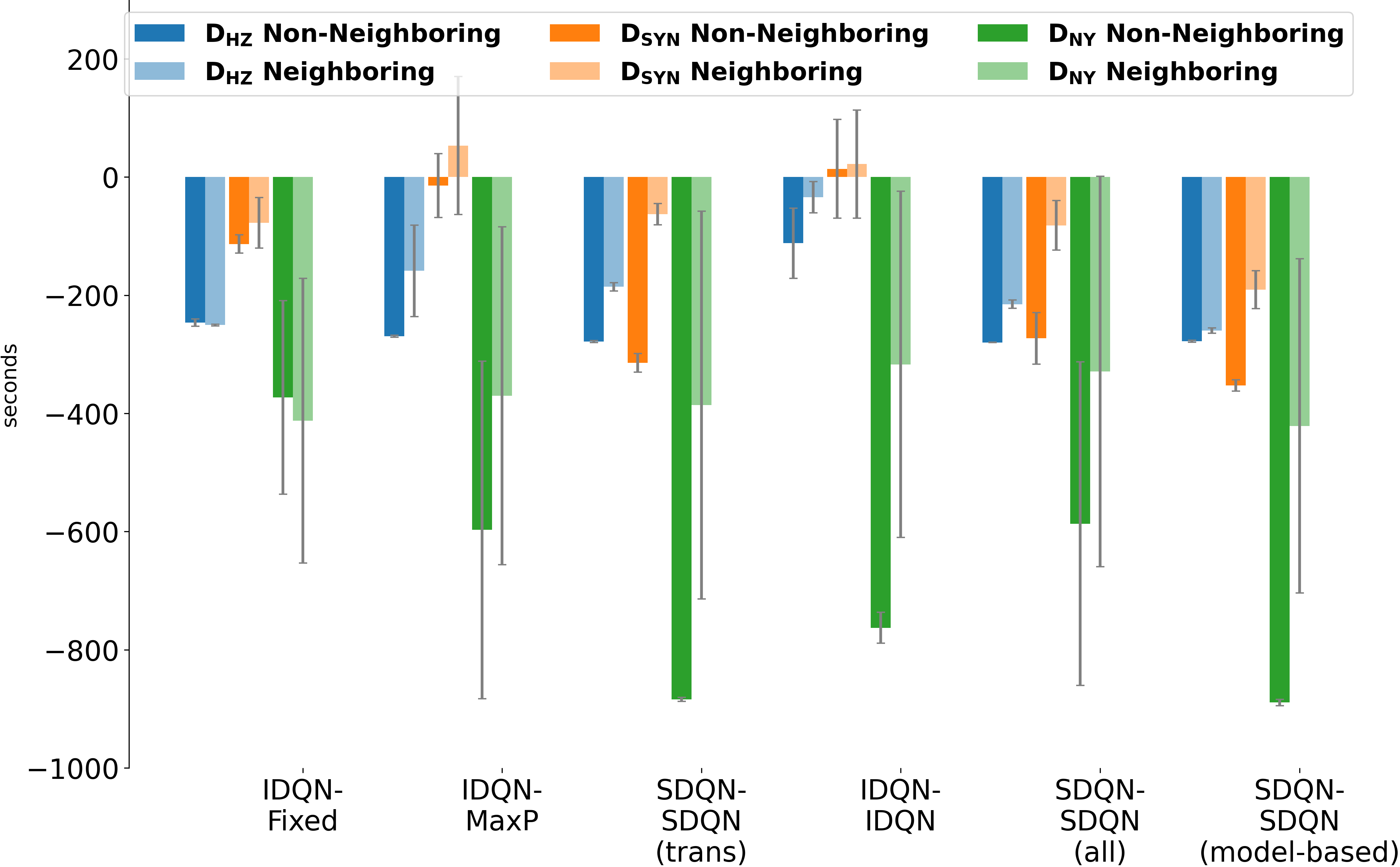
Figure 3: The decrease of average travel time for six control approaches over Fix-Fix (conventional 1) with missing data at non-neighboring and neighboring intersections under all three datasets. The more negative the value is, the better. Each group on X-axis represents a method. Within each group, three colors represent three datasets, where light- and dark-colored bars indicate scenarios with and without adjacent unobserved intersections, respectively. Our proposed method outperforms the Fix-Fix method in most cases.

$\bullet$ Remedy 2.2: SDQN-SDQN (all). Similar to IDQN-IDQN, this method also has a state imputation model and a reward imputation model, while it only trains one shared policy using the observed data from $\mathcal{N}_{o}\$and imputed data from $\mathcal{N}_{m}\$.

$\bullet$ Remedy 2.3: SDQN-SDQN (model-based). This method integrates SDQN-SDQN (all) approaches into MBRL framework. During training, the SDQN agents learn from experiences at all intersections and, at the same time, the reward inference model predicts reward at $\mathcal{N}_{m}$. Different from SDQN-SDQN (all), the reward model is updated upon new experiments returned from the environment; it also has an imaginary rollout phase, during which SDQN agents learn from both states $s_{t}^{j}$ at $\mathcal{N}_{o}\$and imputed states $\hat{s}_{t}^{k}$ at $\mathcal{N}_{m}\$and inferred rewards $\hat{r}_{t}^{i}$ from the updated reward model.

5.2 Overall Performance

We perform experiments to investigate how different approaches perform under different missing rates. The results can be found in Table 1. We have the following observations:

$\bullet$ Compared with Fix-Fix, optimizing IDQN agents at $\mathcal{N}_{o}\$can significantly reduce the average travel time. This validates the effectiveness of RL agents over pre-timed agents.

$\bullet$ Compared with IDQN-Fix, IDQN-Neighboring works worse even at the most ideal settings and cannot converge at higher missing rates, which proves optimizing IDQN agents with no imputation cannot solve the missing data problem.

$\bullet$ IDQN-IDQN method in Remedy 2 does not outperform the original naive method. This is because, in this approach, all agents on $\mathcal{N}_{m}\$are only trained with imputed data which could bring in large uncertainty.

$\bullet$ SDQN-SDQN (model-based), SDQN-SDQN (all), SDQN-SDQN (transferred), and IDQN-MaxP approaches achieve better performances than naive IDQN-Fix approach under all three datasets. This proves the effectiveness of our two-step imputation and control method. As the missing rate increases, their performance decreases. For shared-parameter methods, when the missing rate is moderate, the overall performance is not greatly affected. This is because the shared agent can learn from the experience in both $\mathcal{N}_{o}$ and $\mathcal{N}_{m}$ and make policy stable and easy to converge. More detailed intersection-level metrics can be found in Appendix A.3.

5.3 Data Sparsity Analysis

In this section, we investigate how different missing rate and the location of unobserved intersections influences the performance of the proposed methods.

$\bullet$ Influence of different missing rates. We randomly sample 1,2,3,4 intersections from 16 intersections in the $D_{HZ}$ and $D_{SYN}$ and 3,6,9,12 intersections from 48 intersections in the $D_{NY}$ as unobserved intersections. The results in Table 1 and Figure 2 show that when there are no neighboring unobserved intersections, IDQN-MaxP, SDQN-SDQN (transferred), and SDQN-SDQN (all), SDQN-SDQN (model-based) achieve consistent better performances than Fix-Fix. The performances of the four approaches decrease as the number of unobserved intersections increases. Moreover, the three shared-parameter methods are more stable in performance improvement when the missing rates increase.

$\bullet$ Influence of unobserved locations. In the previous experiments, the unobserved intersections are not adjacent to each other. Here we investigate how the locations of unobserved intersections influence the performance. We conduct experiments on situations where adjacent intersections are unobserved. We randomly sample missing intersections and make sure the network has two unobserved intersections adjacent. The result is shown in Figure 3. We have the following observations: (1) When there are adjacent unobserved intersections, our proposed method still outperforms the Fix-Fix method in most cases. Specifically, SDQN-SDQN (transferred), SDQN-SDQN (all), and SDQN-SDQN (model-based) perform consistently better than other baseline methods. (2) Except for IDQN-Fix, the performance of all other methods drops from non-neighboring scenarios to neighboring scenarios. This is likely because the performance of the control method relies on the imputation method, and missing data at neighboring intersections could negatively affect the performance of the imputation.

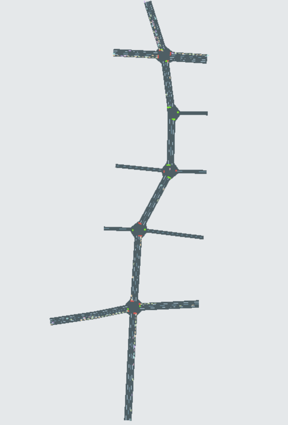
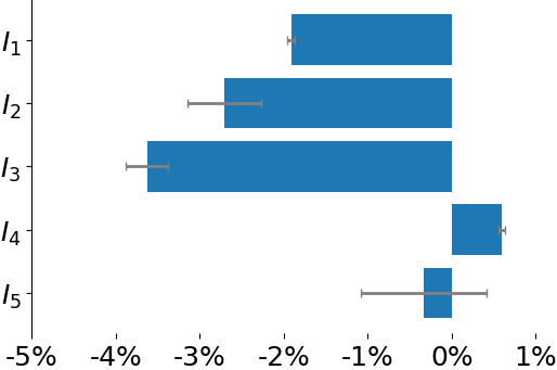
(a) $D_{AL}$ road network	(b) Performance on $D_{AL}$

Figure 4: (a) The topology of $D_{AL}$ network. (b) The decrease of averaged lane delays at each intersection between Fix-Fix and SDQN-SDQN (transferred) under one missing position. The more negative, the better. Other methods are shown in Appendix Figure 9

We also investigated the influence of missing data at frequently visited intersections and found no obvious performance drop when busy intersections are unobserved. The detailed results can be found in Appendix 7.

5.4 Extension on Heterogeneous Intersections

In this section, we investigate our methods under heterogeneous intersections, $D_{AL}$, to see the applicability of our proposed method under the real-world setting. $D_{AL}$ is a public traffic dataset collected in Atlanta, GA, within $1\times 5$ intersections. The intersections have different numbers of lanes and phases, leading to different state spaces for each agent. We use FRAP  Zheng et al. (2019), an RL model proven effective on heterogeneous structure road networks, as our base RL model for SDQN-SDQN to cope with the different input dimensions of heterogeneous intersections. In this experiment, multiple runs are conducted, where each run has a random intersection selected as the unobserved intersection. We find the shared agent outperforms the baseline Fix-Fix method and reduces overall average travel time from 986.36 seconds (Fix-Fix) to 838.45 seconds. The detailed results in Figure 4 (b) show intersection-level average travel time in most intersections is reduced with our proposed method.

6 Conclusion and Future Work

In this paper, we investigate the traffic signal control problem in a real-world setting where the traffic condition around certain locations is missing. To tackle the missing data challenge, we propose two solutions: the first solution is to impute the state at missing intersections and directly use them to help agents at missing intersections make decisions; the second solution is to impute both state and reward and use the imputed experiences to train agents. We conduct extensive experiments using synthetic and real-world data and demonstrate the superior performance of our proposed methods over conventional methods. In addition, we show in-depth case studies and observations to understand how missing data influences the final control performance.

We would also like to point out several future works. First, missing data at neighboring intersections brings a considerable challenge to the imputation model. Future work could explore different imputation methods to improve imputation accuracy. Another direction is to combine our imputation model with more external data like speed data to make the imputation more accurate and improve control performance.

Appendix A Appendix

A.1 Summary of Different Approaches

We analyze and summarize all approaches in the Table 2, Generally, fixed-time methods (e.g., Fix-Fix, IDQN-Fix) do not rely on observations and cannot adapt well to dynamic traffic; shared RL methods (e.g., SDQN-SDQN) using Centralized Training and Decentralized Execution (CTDE) usually perform better than individual RL (e.g., IDQN), particularly with more agents, as validated by Chen et al. [2020]. SDQN-SDQN (transferred) in Remedy 1 uses control models only trained on observed intersections, which may underperform when deployed on unobserved intersections. SDQN-SDQN (all) in Remedy 2 pre-trains an additional reward model, enabling the update of the control model for unobserved intersections, thus mitigating performance issues. SDQN-SDQN (model-based) further refines the reward model training, enhancing the control model’s performance.

Table 2: Summary of advantages and disadvantages of different approaches

Remedy	Approach	Advantage
Convention	Fix-Fix	The control model does not rely on imputation.
	IDQN-Fix	1. All the control models do not rely on imputation. 2. IDQN is adaptive in observed intersections.
Remedy 1	IDQN-MaxP	1. Remedy 1 approaches enable adaptive control in unobserved intersections. 2. Unlike Remedy 2, Remedy 1 approaches do not require a reward imputation model.
	SDQN-SDQN (transferred)	1. Remedy 1 approaches enable adaptive control in unobserved intersections. 2. Unlike Remedy 2, Remedy 1 approaches do not require a reward imputation model. 3. SDQN uses CTDE and converges faster in training the control models.
Remedy 2	IDQN-IDQN	Remedy 2 approaches enable the training of the control model on unobserved intersections.
	SDQN-SDQN (all)	1. Remedy 2 approaches enable the training of the control model on unobserved intersections. 2. SDQN uses CTDE and converges faster in training the control models.
	SDQN-SDQN (model-based)	1. Remedy 2 approaches enable the training of the control model on unobserved intersections. 2. SDQN uses CTDE and converges faster in training the control models. 3. This method can alleviate the data-shifting problem by updating the reward model.
		Disadvatage
Convention	Fix-Fix	Fixed-time agents are not adaptive to dynamic traffic.
	IDQN-Fix	Fixed-time agents are not adaptive to dynamic traffic.
Remedy 1	IDQN-MaxP	1. Remedy 1 approaches require additional training on the state imputation model. 2. MaxPrusure is rule-based and has limited performance under complex traffic. 3. IDQN is hard to converge with multiple agents.
	SDQN-SDQN (transferred)	1. Remedy 1 approaches require additional training on the state imputation model. 2. Control models are not trained on imputed unobserved intersections.
Remedy 2	IDQN-IDQN	1. Remedy 2 approaches require additional training on reward imputation models. 2. IDQN is hard to converge with multiple agents. 3. Pretrained reward models might be biased between observed and unobserved intersections.
	SDQN-SDQN (all)	1. Remedy 2 approaches require additional training on reward imputation models. 2. Pretrained reward models might be biased between observed and unobserved intersections.
	SDQN-SDQN (model-based)	Remedy 2 approaches require additional training on reward imputation models.

A.2 Comparison of Different Imputation Models

To investigate how different imputation models work with our proposed methods, we compare the SFM model with GraphWN, originally used for traffic forecasting problems, and use SDQN-SDQN (transferred) as the control method. Then we conduct experiments under different missing rates to explore different imputation models’ performance on $D_{HZ}$. The result in Fig 5 shows that at low missing rates, two imputation models achieve better performance than Fix-Fix (conventional 1). With the missing rate increases, the two imputation model’s performance drops. We also find the SFM model’s performance degrades slower than the GraphWN method, though GrpahWN achieves better performance at lower missing rates. This shows that compared to learning neural networks, the rule-based SFM model performs more stable under high missing rates. And neural networks are potentially more effective, while they need more complete data.

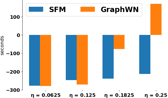
Figure 5: The decrease of two imputation models under different missing rates over Fix-Fix (conventional 1), w.r.t. the average travel time. The lower, the better

A.3 Performance of Different Control Methods on Individual Intersection

To explore how different control methods perform at the intersection level, we also report lane delay at each intersection and investigate different methods’ influences. We randomly sample (1,4), (2,3), and (4,3) out of 16 positions as $\mathcal{N}_{m}\$and report lane delay. The result is shown in Figure 6. We find IDQN-Fix approach can reduce delay at all $\mathcal{N}_{o}\$, but the optimization is limited. IDQN-MaxP and IDQN-IDQN can significantly reduce lane delay at $\mathcal{N}_{o}\$. However, these two approaches also cause negative effects on $\mathcal{N}_{m}\$. This may be because of the imputation error at $\mathcal{N}_{o}\$, which significantly impairs RL-based and rule-based agents’ decisions. For three approaches with parameter-sharing agents, though agents at $\mathcal{N}_{o}\$cannot achieve optimal value, compared to Fix-Fix and IDQN-Fix approaches, delay at most intersections, including $\mathcal{N}_{m}\$are reduced.

(a) IDQN-Fix

(b) IDQN-MaxP

(c) SDQN-SDQN (transferred)

(d) IDQN-IDQN

(e) SDQN-SDQN (all)

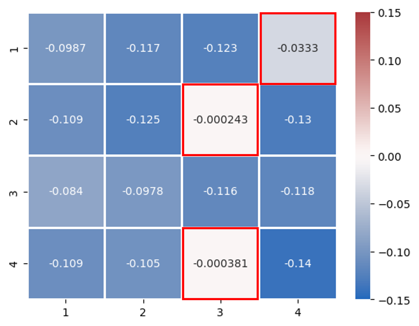
(f) SDQN-SDQN (model)

Figure 6: The decrease of delay for six control approaches over Fix-Fix control method (conventional 1) with unobserved intersections at (1,4), (2,3), (4,3) marked with red rectangle. The more negative, the better performance compared to Fix-Fix control at each intersection.

A.4 Influences of Unobserved Intersections at Frequently Visited Positions

In traffic signal control, averages can hide adverse effects on sparsely visited intersections. We thus delve into a real-world dataset and investigate the effect of frequently visited intersections is unobserved. The total visited vehicle counts are shown in Figure 7.

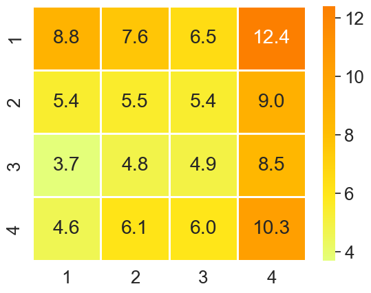
Figure 7: Total number of vehicles visited at each intersection (hundreds) in $D_{HZ}$. The higher number of visited vehicles means this intersection is busier and more important in the traffic.

$\bullet$ Missing positions at frequently visited areas. We sampled 3 groups of intersections, each has 3 out of 16 unobserved intersections, and tested different approaches’ performance. The result is shown in Table 3. Comparing the average travel time of different approaches under the first two groups of intersections (not frequently visited) and the last group of intersections (frequently visited), we found no significant deprecation.

The Last group includes one most visited intersections; the other two do not. Across the comparison between different imputation approaches, we find our methods are robust to this challenge.

Table 3: Unobserved intersections allocated at different frequent vehicle visited positions. Frequently visited intersections are highlighted

MISSING POSITION	IDQN-Fix	IDQN-MaxP	SDQN-SDQN (transferred)	IDQN-IDQN	SDQN-SDQN (all)	SDQN-SDQN (model-based)
(2,1), (2,4), (4,1)	367.43	344.24	331.53	457.86	332.76	330.53
(1,1), ( 3,1), (3,4)	369.47	343.42	338.07	581.97	330.18	336.05
(1,4), (2,3), (4,3)	373.63	340.04	326.98	573.73	327.88	409.04

A.5 Heterogeneous Road Network Topology

The dataset $D_{AL}$ we used in Sec. 5.4 has a highly heterogeneous topology. It has 3 different configurations in total. Intersections 1 and 5 have eight lanes and four phases. Intersection 2 has five lanes and one phase, and intersections 3 and 4 have six lanes and two phases.

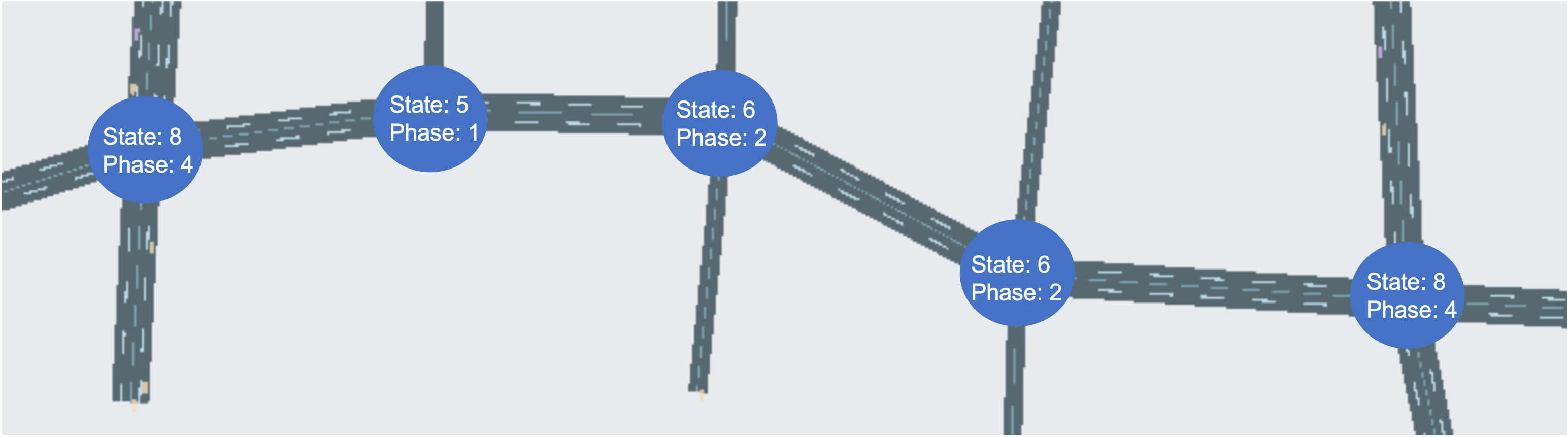
Figure 8: Topology of $D_{AL}$. It has 5 intersections with different states and phases. Indexes are 1 to 5 from left to right.

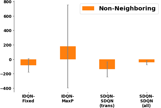
Figure 9: The decrease of average travel time for four control approaches over the Fix-Fix control method (conventional 1) with missing data at one intersection. The more negative the value is, the better. IDQN-Fix, SDQN-SDQN (transferred), and SDQN-SDQN (all) perform better than Fix-Fix. And SDQN-SDQN (transferred) performs best among all

We test our proposed methods on this heterogeneous structure network. The complete result of average travel time is shown in Figure 9 as support for the lane level result shown in Sec.5.4. We found SDQN-SDQN (transferred) control method performs best, which supports the effectiveness of our proposed methods. Also, with parameter-sharing, our proposed two-step imputation methods are applicable to complex real-world scenarios.

A.6 Base Model Analysis

We use DQN Wei et al. [2018] as our base model in the previous sections. To investigate the influences of the base model on the final performance, we conducted experiments using different RL models (i.e., FRAP Zheng et al. [2019], Dueling DQN Moerland et al. [2020]; Khalili et al. [2021]) under the dataset $D_{HZ}$.

Table 4 shows the performance comparison of the change on the base models with the DQN model w.r.t. average travel time. It can be observed that Dueling DQN can achieve better results than DQN in most cases. For other base models that are reported to be better than DQN, it is expected to improve the performance of our proposed method as well.

Table 4: $\Delta$ average travel time means reduced average travel time of FRAP and Dueling-DQN agents compared with DQN on $D_{HZ}$. Negative results show that with FRAP and Dueling DQN as RL agents, average travel time is reduced compared to DQN agents. We highlighted results with $\Delta$ average travel time less than zero.

METHOD	MISSING RATE	$\Delta$ Average Travel Time
		FRAP	Dueling DQN
IDQN-Fix	6.25%	+32.0157	-4.9868
IDQN-MaxP		+53.7521	+11.1077
SDQN-SDQN (transferred)		+25.736	-1.6961
IDQN-IDQN		-22.8162	-67.5349
SDQN-SDQN (all)		+22.4184	-0.1957
SDQN-SDQN (model-based)		+25.381	-1.7308
IDQN-Fix	12.5%	+8.1247	-16.7985
IDQN-MaxP		+23.5246	-53.4985
SDQN-SDQN (transferred)		+31.198	+17.7471
IDQN-IDQN		+60.4042	-42.4859
SDQN-SDQN (all)		+10.3246	+13.1825
SDQN-SDQN (model-based)		+7.532	+1.2769
IDQN-Fix	18.75%	+12.0974	-14.1713
IDQN-MaxP		+45.5611	-11.9744
SDQN-SDQN (transferred)		-10.5883	-14.7092
IDQN-IDQN		-16.7969	-55.5823
SDQN-SDQN (all)		-5.1507	-0.4848
SDQN-SDQN (model-based)		+66.0515	-10.573
IDQN-Fix	25%	-14.1858	-31.6266
IDQN-MaxP		+107.4302	+6.8059
SDQN-SDQN (transferred)		+43.8644	-12.0765
IDQN-IDQN		+49.406	-78.5265
SDQN-SDQN (all)		-6.9524	-9.9602
SDQN-SDQN (model-based)		-12.8496	-26.5348

References

- Aboudolas et al. [2009] K. Aboudolas, M. Papageorgiou, and E. Kosmatopoulos. Store-and-forward based methods for the signal control problem in large-scale congested urban road networks. Transportation Research Part C: Emerging Technologies, 17(2):163–174, 2009. Selected papers from the Sixth Triennial Symposium on Transportation Analysis (TRISTAN VI).
- Arel et al. [2010] Itamar Arel, Cong Liu, Tom Urbanik, and Airton G Kohls. Reinforcement learning-based multi-agent system for network traffic signal control. IET Intelligent Transport Systems, 4(2):128–135, 2010.
- Chen and Jiang [2019] Jinglin Chen and Nan Jiang. Information-theoretic considerations in batch reinforcement learning. In International Conference on Machine Learning, pages 1042–1051. PMLR, 2019.
- Chen et al. [2019] Xinyu Chen, Zhaocheng He, and Lijun Sun. A bayesian tensor decomposition approach for spatiotemporal traffic data imputation. Transportation Research Part C: Emerging Technologies, 98:73–84, 2019.
- Chen et al. [2020] Chacha Chen, Hua Wei, Nan Xu, Guanjie Zheng, Ming Yang, Yuanhao Xiong, Kai Xu, and Zhenhui Li. Toward a thousand lights: Decentralized deep reinforcement learning for large-scale traffic signal control. In Proceedings of the AAAI Conference on Artificial Intelligence, volume 34, pages 3414–3421, 2020.
- Cui et al. [2020] Zhiyong Cui, Ruimin Ke, Ziyuan Pu, and Yinhai Wang. Stacked bidirectional and unidirectional lstm recurrent neural network for forecasting network-wide traffic state with missing values. Transportation Research Part C: Emerging Technologies, 118:102674, 2020.
- Duan et al. [2016] Yanjie Duan, Yisheng Lv, Yu-Liang Liu, and Fei-Yue Wang. An efficient realization of deep learning for traffic data imputation. Transportation Research Part C: Emerging Technologies, 72:168–181, 2016.
- El-Tantawy et al. [2013] Samah El-Tantawy, Baher Abdulhai, and Hossam Abdelgawad. Multiagent reinforcement learning for integrated network of adaptive traffic signal controllers (marlin-atsc): methodology and large-scale application on downtown toronto. IEEE Transactions on Intelligent Transportation Systems, 14(3):1140–1150, 2013.
- Gan et al. [2015] Min Gan, C. L. Philip Chen, Han-Xiong Li, and Long Chen. Gradient radial basis function based varying-coefficient autoregressive model for nonlinear and nonstationary time series. IEEE Signal Processing Letters, 22(7):809–812, 2015.
- Huang et al. [2021] Xingshuai Huang, Di Wu, Michael Jenkin, and Benoit Boulet. Modellight: Model-based meta-reinforcement learning for traffic signal control. arXiv preprint arXiv:2111.08067, 2021.
- Hunt et al. [1981] PB Hunt, DI Robertson, RD Bretherton, and RI Winton. Scoot-a traffic responsive method of coordinating signals. Technical report, 1981.
- Khalili et al. [2021] Ata Khalili, Ehsan Mohammadi Monfard, Shayan Zargari, Mohammad Reza Javan, Nader Mokari, and Eduard A. Jorswieck. Resource management for transmit power minimization in uav-assisted RIS hetnets supported by dual connectivity. CoRR, abs/2106.13174, 2021.
- Koonce and Rodegerdts [2008] Peter Koonce and Lee Rodegerdts. Traffic signal timing manual. Technical report, United States. Federal Highway Administration, 2008.
- Li et al. [2020] Xiaoshuang Li, Zhongzheng Guo, Xingyuan Dai, Yilun Lin, Junchen Jin, Fenghua Zhu, and Fei-Yue Wang. Deep imitation learning for traffic signal control and operations based on graph convolutional neural networks. In 2020 IEEE 23rd International Conference on Intelligent Transportation Systems (ITSC), pages 1–6. IEEE, 2020.
- Luo et al. [2022] Fan-Ming Luo, Tian Xu, Hang Lai, Xiong-Hui Chen, Weinan Zhang, and Yang Yu. A survey on model-based reinforcement learning, 2022.
- Lv et al. [2015] Yisheng Lv, Yanjie Duan, Wenwen Kang, Zhengxi Li, and Fei-Yue Wang. Traffic flow prediction with big data: A deep learning approach. IEEE Transactions on Intelligent Transportation Systems, 16(2):865–873, 2015.
- Mai et al. [2019] Tien Mai, Quoc Phong Nguyen, Kian Hsiang Low, and Patrick Jaillet. Inverse reinforcement learning with missing data. arXiv preprint arXiv:1911.06930, 2019.
- Moerland et al. [2020] Thomas M. Moerland, Joost Broekens, and Catholijn M. Jonker. Model-based reinforcement learning: A survey. CoRR, abs/2006.16712, 2020.
- Oroojlooy et al. [2020] Afshin Oroojlooy, Mohammadreza Nazari, Davood Hajinezhad, and Jorge Silva. Attendlight: Universal attention-based reinforcement learning model for traffic signal control. Advances in Neural Information Processing Systems, 33:4079–4090, 2020.
- Sims and Dobinson [1980] Arthur G Sims and Kenneth W Dobinson. The sydney coordinated adaptive traffic (scat) system philosophy and benefits. IEEE Transactions on vehicular technology, 29(2):130–137, 1980.
- Sutton [1991] Richard S Sutton. Dyna, an integrated architecture for learning, planning, and reacting. ACM Sigart Bulletin, 2(4):160–163, 1991.
- Terry et al. [2020] J. K. Terry, Nathaniel Grammel, Sanghyun Son, and Benjamin Black. Parameter sharing for heterogeneous agents in multi-agent reinforcement learning, 2020.
- Tirone [2022] Onathan Tirone. Congestion pricing, the route more cities are taking. Bloomberg, 2022.
- Varaiya [2013] Pravin Varaiya. The max-pressure controller for arbitrary networks of signalized intersections. In Advances in dynamic network modeling in complex transportation systems, pages 27–66. Springer, 2013.
- Wang et al. [2022] Peixiao Wang, Tong Zhang, Yueming Zheng, and Tao Hu. A multi-view bidirectional spatiotemporal graph network for urban traffic flow imputation. International Journal of Geographical Information Science, 36(6):1231–1257, 2022.
- Wei et al. [2018] Hua Wei, Guanjie Zheng, Huaxiu Yao, and Zhenhui Li. Intellilight: A reinforcement learning approach for intelligent traffic light control. In Proceedings of the 24th ACM SIGKDD International Conference on Knowledge Discovery & Data Mining, pages 2496–2505, 2018.
- Wei et al. [2019a] Hua Wei, Chacha Chen, Guanjie Zheng, Kan Wu, Vikash Gayah, Kai Xu, and Zhenhui Li. Presslight: Learning max pressure control to coordinate traffic signals in arterial network. In Proceedings of the 25th ACM SIGKDD International Conference on Knowledge Discovery & Data Mining, KDD ’19, pages 1290–1298, 2019.
- Wei et al. [2019b] Hua Wei, Nan Xu, Huichu Zhang, Guanjie Zheng, Xinshi Zang, Chacha Chen, Weinan Zhang, Yanmin Zhu, Kai Xu, and Zhenhui Li. Colight: Learning network-level cooperation for traffic signal control. In Proceedings of the 28th ACM International Conference on Information and Knowledge Management, pages 1913–1922, 2019.
- Wu et al. [2019] Zonghan Wu, Shirui Pan, Guodong Long, Jing Jiang, and Chengqi Zhang. Graph wavenet for deep spatial-temporal graph modeling. arXiv preprint arXiv:1906.00121, 2019.
- Wu et al. [2021] Libing Wu, Min Wang, Dan Wu, and Jia Wu. Dynstgat: Dynamic spatial-temporal graph attention network for traffic signal control. In Proceedings of the 30th ACM International Conference on Information & Knowledge Management, pages 2150–2159, 2021.
- Yao et al. [2018] Huaxiu Yao, Fei Wu, Jintao Ke, Xianfeng Tang, Yitian Jia, Siyu Lu, Pinghua Gong, Jieping Ye, and Zhenhui Li. Deep multi-view spatial-temporal network for taxi demand prediction. Proceedings of the AAAI Conference on Artificial Intelligence, 32(1), Apr. 2018.
- Zhang et al. [2019] Huichu Zhang, Siyuan Feng, Chang Liu, Yaoyao Ding, Yichen Zhu, Zihan Zhou, Weinan Zhang, Yong Yu, Haiming Jin, and Zhenhui Li. Cityflow: A multi-agent reinforcement learning environment for large scale city traffic scenario. In The world wide web conference, pages 3620–3624, 2019.
- Zhang et al. [2021] Weibin Zhang, Pulin Zhang, Yinghao Yu, Xiying Li, Salvatore Antonio Biancardo, and Junyi Zhang. Missing data repairs for traffic flow with self-attention generative adversarial imputation net. IEEE Transactions on Intelligent Transportation Systems, 2021.
- Zhao et al. [2020] Yangyang Zhao, Zhenyu Wang, Kai Yin, Rui Zhang, Zhenhua Huang, and Pei Wang. Dynamic reward-based dueling deep dyna-q: Robust policy learning in noisy environments. In Proceedings of the AAAI Conference on Artificial Intelligence, volume 34, pages 9676–9684, 2020.
- Zheng et al. [2019] Guanjie Zheng, Yuanhao Xiong, Xinshi Zang, Jie Feng, Hua Wei, Huichu Zhang, Yong Li, Kai Xu, and Zhenhui Li. Learning phase competition for traffic signal control. CoRR, abs/1905.04722, 2019.
- Zhong et al. [2004] Ming Zhong, Pawan Lingras, and Satish Sharma. Estimation of missing traffic counts using factor, genetic, neural, and regression techniques. Transportation Research Part C: Emerging Technologies, 12(2):139–166, 2004.