Conservative Sparse Neural Network Embedded Frequency-Constrained Unit Commitment
With Distributed Energy Resources

Abstract

The increasing penetration of distributed energy resources (DERs) will decrease the rotational inertia of the power system and further degrade the system frequency stability. To address the above issues, this paper leverages the advanced neural network (NN) to learn the frequency dynamics and incorporates NN to facilitate system reliable operation. This paper proposes the conservative sparse neural network (CSNN) embedded frequency-constrained unit commitment (FCUC) with converter-based DERs, including the learning and optimization stages. In the learning stage, it samples the inertia parameters, calculates the corresponding frequency, and characterizes the stability region of the sampled parameters using the convex hulls to ensure stability and avoid extrapolation. For conservativeness, the positive prediction error penalty is added to the loss function to prevent possible frequency requirement violation. For the sparsity, the NN topology pruning is employed to eliminate unnecessary connections for solving acceleration. In the optimization stage, the trained CSNN is transformed into mixed-integer linear constraints using the big-M method and then incorporated to establish the data-enhanced model. The case study verifies 1) the effectiveness of the proposed model in terms of high accuracy, fewer parameters, and significant solving acceleration; 2) the stable system operation against frequency violation under contingency.

Nomenclature

The main notation below is provided for unit commitment problem formulation. And other additional symbols are defined in the paper when needed.

A. Sets and Indices

$t\in\mathcal{T}$

Set of the time periods.

$g\in\mathcal{G}$

Set of the thermal generators.

$n\in\mathcal{N}$

Set of the system buses.

$w\in\mathcal{W}$

Set of the converter-based wind turbine generators.

$pv\in\mathcal{PV}$

Set of the converter-based PV generators.

$j\in\mathcal{N}_{d}$

Set of the droop control converters.

$k\in\mathcal{N}_{v}$

Set of the VSM control converters.

B. Decision Variables

$x_{g,t}^{SU}/x_{g,t}^{SD}$

Indicators of units start up / shunt down.

$x_{g,t}$

Operation status of units.

$p_{g,t}/p_{w,t}/p_{pv,t}$

Power output of thermal, wind turbines, and PV generators.

$p^{cur}_{n,t}$

Load curtailment of the bus node.

$u_{gi}/u_{dj}/u_{dk}$

Frequency response participation indicators of the thermal generators, droop / VSM converters.

$M$

System aggregate inertia constant.

$D$

System aggregate damping constant.

$R_{g}$

System aggregate droop factor.

$F_{g}$

System aggregate fraction factor.

$\delta$

Phase angle of the bus node.

$P_{ij}$

Power flow between node $i$ and node $j$.

C. Parameters

$f_{N}$

Nominal frequency rating value.

$f^{min}/f_{lim}(t_{j,t})$

Minimum frequency limits / stepwise frequency limit.

$C_{oper}/C_{rsv}/C_{load}$

Costs of system operation / reserve / load reduction.

$B_{mn}$

The susceptance of the transmission line.

$\hat{p}_{w,t}/\hat{p}_{pv,t}$

Day-ahead predicted power of wind / PV.

$M_{gi}$

Inertia constant of the unit $i$.

$D_{gi}$

Damping constant of the unit $i$.

$R_{gi}$

Inertia constant of the unit $i$.

$K_{gi}$

Mechanical power gain of the unit $i$.

$F_{gi}$

Fraction of the unit $i$ power generation by the turbine.

$R_{dj}$

Droop gain of the converter $j$.

$K_{dj}$

Mechanical power gain of the converter $j$.

$M_{dk}$

Virtual inertia of the converter $k$.

$D_{dk}$

Virtual damp constant of the converter $k$.

$\epsilon_{l}/\epsilon_{der}$

Prediction errors of load and DERs.

I Introduction

In the transition to a low carbon energy society, the renewable energies are replacing the conventional fossil energies and taking up a larger proportion of generation in the modern power system [1]. Unlike the direct connection of fossil-based synchronous generators, the distributed energy resources (DERs) are integrated into the grid through power converters that lack inherent rotational inertia, leading to the low-inertia systems [2]. The decreased rotational inertia will degrade the frequency stability of the system or even trigger large-scale blackouts [4, 3].

To address the above frequency stability problems of the low-inertia systems, the system operator should consider the frequency dynamics under contingency, transform the frequency dynamics requirements into static operational constraints, and incorporate them into the upstream scheduling models. Current research has focused on the formulation and incorporation of the frequency constraints by approximating the frequency nadir, which can be categorized into two types. The first type approximates the frequency response of generators as a piece-wise linear function to time, decoupling the governor control from the frequency in Ref. [5, 6, 7, 8]. Though exhibiting a simplified form with the frequency nadir constraints, it ignores the actual control policy and may not apply to high penetrated converter-based DER scenarios. The second type is based on the system frequency response model combined with the converter response feature to formulate the total frequency dynamics in Ref. [9, 10, 12, 11]. Ref. [9, 10] derive the analytical expression of frequency dynamics with converter-based DERs, calculate the frequency nadir expression, and utilize the piece-wise linear formulation to approximate these dynamics, which can be converted into a set of linear constraints. Ref. [11] further considers the joint scheduling of wind farm frequency support and reserve based on the analytical expression. These piece-wise linear models include the converter-based DER response but have limited approximation capability, which may not satisfy the requirement of complex converter-based power systems [13, 14].

The frequency support potential of the high-penetration DERs has been explored and exploited within the control scheme of the grid-forming voltage source converter (VSC) [16, 15, 17]. Virtual synchronous machine policy is one of the common VSC control strategies based on the emulation of system inertia [15]. Ref. [16] proposes a generalized architecture of VSC from the view of multivariable feedback control to unify different control strategies. Ref. [17] focuses on the wind turbine generators and proposes multiple virtual rotating masses for frequency support. However, the direct inertia parameter aggregation of different VSC control methods may lead to the low-inertia system instability [2].

So the relationship between the frequency dynamics and frequency support sources under the high penetrated converter-based DER is governed by the system’s ordinary differential equations, which are complicated and cannot be incorporated into the system operation model directly. The thriving machine learning (ML) technique, widely applied in pattern cognition [18, 19] and image detection [20, 21], provides the powerful deep neural networks (DNNs) to formulate the above relationship with high accuracy [22, 23, 24, 25, 26]. The enforced constraints on the DNN-based frequency can be transformed into the mixed-integer linear programming [27] and solved efficiently by the off-the-shelf solvers [25]. In Ref. [22], the DNN is utilized to learn constraints and objectives, and the learned DNN is embedded in solving the world food program planning problem. |Two critical issues arises from the direct integration of the trained DNNs into the frequency-constrained scheduling models will raise : 1) the positive and negative prediction errors of a DNN have different impacts on the system, where positive errors can lead to violations of the frequency requirements, and 2) the parameter number of the conventional dense DNN can be huge, resulting in the long solving time [28].

Faced with the complex frequency dynamics under the high penetrated converter-based DERs, this paper leverages the advanced research in ML and the dramatic improvement in solving mixed-integer linear programming (MILP) to formulate and incorporate the frequency constraints into operation models to ensure the system stable operation. To address the issues of DNN integration, it proposes the conservative sparse neural network (CSNN) embedded frequency-constrained unit commitment model with DER, composed of learning and optimization stages. Its key lies in the design of the CSNN to achieve the conservativeness and sparsity of NN, which can further facilitate the safety and efficiency of CSNN incorporation. It first formulates and derives the highly non-convex frequency dynamics explicitly under DER. In the learning stage, it samples the inertia parameters, calculates the corresponding frequency, and characterizes the stability region of the sampled parameters using the convex hull to ensure stability and avoid extrapolation. Then for the conservativeness of NN, the positive prediction error penalty is added to the loss function to avoid possible frequency requirement violation; for the sparsity of NN, the neural network topology pruning is employed in training NN to eliminate some unnecessary connections for achieving MILP solving acceleration. In the optimization stage, the trained CSNN is transformed into a series of mixed-integer linear constraints using the big-M method to relax the ReLU activation functions in NN. Then these frequency constraints is incorporated into the conventional unit commitment (UC) to establish the final data-enhanced frequency constrained UC model in the MILP form. For this paper, the main contributions are as follows:

1) To the best of authors’ knowledge, this paper, for the first time, proposes the conservative sparse neural network to achieve both the conservativeness and sparsity of neural networks, which is beneficial to NN embedding in the optimization problems and can be utilized to formulate the relationship between the frequency dynamics and system inertia parameters. The proposed CSNN achieves higher approximation accuracy, compared with the previous piece-wise linear formulation of frequency dynamics in Ref. [15, 10], which exhibits i) fewer parameters to accelerate MILP solving ii) and conservative prediction to prevent the violation of frequency requirements, compared with conventional NN.

2) Based on the proposed CSNN, this paper proposes the data-enhanced frequency constrained unit commitment under DER to address the frequency stability problem of the low-inertia system. The proposed scheduling model approximates both frequency nadir and stepwise constraints by CSNN, transforms the trained CSNNs into a series of mixed-integer linear constraints using the big-M method, and embeds the constraints into the conventional UC model. Compared with conservative and conventional neural networks, the proposed data-enhanced model can achieve significant MILP solution time reduction, verifying its efficiency.

3) This paper designs the stability region using convex hulls from the sampled dataset with stability to guarantee the system operation stability and avoid extrapolation. The main reason for stability region is that not all inertia parameters in the sampled dataset can stabilize the total system, especially under the high penetration of the converter-based DERs. So the inertia parameters with stability are extracted to construct the stable dataset, and then the clustered convex hulls are extracted, denoted by stability region, which are transformed into linear constraints and embedded into the scheduling model to guarantee the stability and feasibility.

For clearer delivery, we further summarize the main motivation and innovation of this paper. The increasing distributed energy resources will decrease the system rotational inertia and further degrade the system frequency stability, which requires the frequency consideration in system scheduling. However, the relationships between frequency dynamics and frequency support sources are complex, which requires the accurate and conservative formulation to capture the relationship. To address the above issues, we propose the CSNN with high representational capacity for capturing the above complex frequency relationship effectively with conservativeness design and embed the trained CSNN into the conventional unit commitment model efficiently with sparsity design to formulate the data-enhanced frequency constrained unit commitment model. The rest of this paper is organized as follows. Section II depicts the frequency dynamics with distributed energy resources. Section III proposes the conservative sparse neural network to formulate the frequency constraints. Section IV presents the CSNN embedded data-enhanced frequency-constrained unit commitment with DER. Section V performs the case study to verify the efficiency of the proposed model. Section VI concludes this paper.

II Frequency Dynamics Formulation with Distributed Energy Resources

This section formulates the system frequency dynamics under conventional synchronous generators and converter-based DER generators mathematically, governed by nonlinear ordinary differential equations from Ref. [30]. The frequency dynamics can be analyzed by the swing equation in Eq. eq: swing.

$$\begin{aligned} M\frac{d\Delta f}{dt}+D\Delta f=\Delta p_{g}-\Delta p_{e}.\end{aligned}$$ (1)

Then, based on Eq. eq: swing, the low-inertia system dynamics is introduced, and several key frequency constraints are proposed to guarantee the frequency dynamic stability.

II-A Frequency Dynamics Analytical Analysis

Based on Ref. [15], we can derive the transfer function $G(s)$ of the system dynamics model in Eq. eq: analytical transfer.

$$\allowdisplaybreaks\begin{aligned} G(s)&=\frac{\Delta f}{\Delta P_{e}}=\Big{(}\underbrace{(sM_{g}+D_{g})+\sum_{i\in\mathcal{N}_{g}}\frac{K_{gi}(1+sF_{gi}T_{gi})}{R_{gi}(1+sT_{gi})}}_{\text{Multiple-machine system frequency response}}\\ &+\underbrace{\sum_{j\in\mathcal{N}_{d}}\frac{K_{cj}}{R_{cj}(1+sT_{cj})}}_{\text{Droop control from DERs}}+\underbrace{\sum_{k\in\mathcal{N}_{v}}\frac{sM_{ck}+D_{ck}}{1+sT_{ck}}}_{\text{VSM control from DERs}}\Big{)}^{-1}.\end{aligned}$$ (2)

It is assumed that all synchronous generators have equal time constants with $T_{gi}=T,\forall i\in\mathcal{N}_{g}$. The time constants of converters are 2-3 orders lower than those of synchronous generators with $T\gg T_{c}\approx 0$, according to Ref. [33]. Then we transform the general-order Eq. eq: analytical transfer into its second-order form Eq. eq: general form.

$$\allowdisplaybreaks\begin{aligned} G(s)=\frac{1}{MT}\frac{1+sT}{s^{2}+2\zeta\omega_{n}s+\omega^{2}_{n}}.\end{aligned}$$ (3)

where $\omega_{n}$ and $\zeta$ denote the natural frequency and damping ratio, calculated by Eq. eq: param cal.

$$\allowdisplaybreaks\begin{aligned} \omega_{n}=\sqrt{\frac{D+R_{g}}{MT}},\quad\zeta=\frac{M+T(D+F_{g})}{2\sqrt{MT(D+R_{g})}}.\end{aligned}$$ (4)

The key parameters $M$, $D$, $F_{g}$, and $R_{g}$ in Eq. eq: param cal calculation can be referred to Ref. [15].

Given a stepwise disturbance $\Delta P$ ($\Delta P/s$ in the frequency domain) in Eq. eq: swing, the frequency dynamics in time domain can be derived from Eq. eq: general form as follows:

$$\allowdisplaybreaks\begin{aligned} \Delta f(t)=&-\frac{\Delta P}{MT\omega^{2}_{n}}\\ &-\frac{\Delta P}{M\omega_{d}}e^{-\zeta\omega_{n}t}\Big{(}\sin(\omega_{d}t)-\frac{1}{\omega_{n}T}\sin(\omega_{d}t+\phi)\Big{)}\end{aligned}$$ (5)

where the $\omega_{d}$ and $\phi$ calculated as follows:

$$\allowdisplaybreaks\begin{aligned} \omega_{d}=\omega_{n}\sqrt{1-\zeta^{2}},\quad\phi=\arcsin(\sqrt{1-\zeta^{2}}).\end{aligned}$$ (6)

The frequency nadir is located in the time instance $t_{m}$ where the derivative of frequency is zero in Eq. eq: t nadir.

$$\allowdisplaybreaks\begin{aligned} \frac{d\Delta f(t_{m})}{t_{m}}=0\rightarrow t_{m}=\frac{1}{\omega_{d}}\tan^{-1}(\frac{\omega_{d}}{\zeta\omega_{n}-T^{-1}}).\end{aligned}$$ (7)

Then the maximum frequency deviation can be calculated by replacing the $t$ of Eq. eq: time domain by $t_{m}$ of Eq. eq: t nadir as:

$$\allowdisplaybreaks\begin{aligned} \Delta f_{max}=-\frac{\Delta P}{D+R_{g}}(1+\sqrt{\frac{T(R_{g}-F_{g})}{M}}e^{-\zeta\omega_{n}t_{m}}).\end{aligned}$$ (8)

II-B Frequency Constraints Formulation

Based on the above analytical frequency response formulation, this paper proposes four key constraints to bound frequency dynamics for securing the system stability from different perspectives, including the rate-of-change-of-frequency (RoCoF) constraint for guaranteeing transient stability [31], the quasi-steady state for bringing back system normal operation state [9], the frequency nadir constraint for avoiding the activation of under frequency load shedding [15], and the stepwise frequency constraint for enhancing the frequency restoration performance[8].

II-B1 RoCoF Constraint

RoCoF constraint guarantees the sufficient system inertia to limit the allowable RoCoF at $t=0$, following the ENTSO-E standard [32].

$$|\text{RoCoF}|=|\frac{\Delta P}{M}|\leq\text{RoCoF}^{max}.$$ (9)

II-B2 Quasi-Steady State Constraint

Quasi-steady state (QSS) constraint guarantees quasi-steady state security assuming the RoCoF is effectively zero.

$$\Delta f_{qss}=-\frac{\Delta P}{D+R_{g}}\leq\Delta f^{max}_{qss}.$$ (10)

II-B3 Frequency Nadir Constraints

To avoid triggering under-frequency load shedding (UFLS) and oscillation, the maximum frequency deviation should be limited within the allowable range by Eq. eq: nadir contrs.

$$f_{nadir}=f_{N}-\Delta f_{max}\geq f^{min}.$$ (11)

II-B4 Frequency Stepwise Constraints

Besides the above frequency constraints, we further consider the frequency restoration requirement from frequency nadir to quasi-steady state, inspired by Ref. [8]. The stepwise frequency constraints are utilized to bound the frequency restoration process, as shown in Eq. eq: mulifreq, Eq. eq: freq stepwise, and Fig. 1.

$$\allowdisplaybreaks\begin{aligned} f_{lim}(t)=\begin{cases}f_{0}\quad&0\leq t<t_{1,l}\\ f_{1}\quad&t_{1,l}\leq t<t_{2,l}\\ \cdots\\ f_{j}\quad&t_{j,l}\leq t<t_{j+1,l}\\ \cdots\\ f_{N_{c}}\quad&t_{N_{c},l}\leq t\end{cases}.\end{aligned}$$ (12)

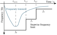
Figure 1: Multiple stepwise frequency requirement.

Then we formulate the stepwise frequency constraints as follows:

$$\allowdisplaybreaks\begin{aligned} f(t)=f_{N}-\Delta f(t)\geq f_{lim}(t).\end{aligned}$$ (13)

However, the above constraints are complicated because they should be evaluated for $t\geq 0$. As shown in Fig. 1, the stepwise frequency constraints are binding when the transient curve and limit curve touch. The constraints are not required when no step changes in the frequency limit curve. So we only evaluate it at the step change time $t=t_{j,l}$ as follows:

$$\allowdisplaybreaks\begin{aligned} f(t_{j,l})=f_{N}-\Delta f(t_{j,l})\geq f_{lim}(t_{j,l})\quad j\in N_{c}.\end{aligned}$$ (14)

II-C Frequency Constraints Analysis

II-C1 Relationship Analysis

The RoCoF and QSS constraints are linear with respect to $M$, $D$, and $R_{g}$. In contrast, the frequency nadir and stepwise constraints are nonlinear due to the nonlinearity of $f_{nadir}(M,D,R_{g},F_{g})$ and $f(M,D,R_{g},F_{g};t_{j,l})$ with respect to $M$, $D$, $R_{g}$, and $F_{g}$.

II-C2 Conservative Approximation of Frequency Constraints

So we need to derive the tractable constraints from the nonlinear ones to facilitate tractable solving. The system operator prioritizes the negative error (predicted value minus true value) but is averse to positive error, where positive errors may result in the frequency requirement violation. So we propose to approximate the $f_{nadir}$ and $f(t_{j,l})$ in a conservative way in Eq. eq: freq conser.

$$f_{nadir}(M,D,R_{g},F_{g})\geq\hat{f}_{nadir}(M,D,R_{g},F_{g})\geq f^{min}$$ (15a)

$$f(M,D,R_{g},F_{g};t_{j,l})\geq\hat{f}(M,D,R_{g},F_{g};t_{j,l})\geq f_{lim}(t_{j,l})$$ (15b)

where $\hat{f}_{nadir}$ and $\hat{f}$ are the predicted frequency, which are the lower bounds of the true frequency.

III Methodology

Based on the frequency constraints formulation and analysis, this section 1) introduces the concept of optimization with constraint learning (OCL) framework, 2) proposes the conservative sparse neural network formulation under the OCL framework for nonlinear frequency constraints in Eq. eq: freq conser, 3) embeds the trained neural network into the optimization models via MILP, 4) and presents two data processing techniques for facilitating predictive model integration.

III-A Data-driven Optimization with Constraint Learning Framework Design

Practical optimization problems often contain constraints with intractable forms or no explicit formulas. However, based on the supportive data corresponding to such constraints, these data can be utilized to learn the constraints (constraint learning, CL). The trained predictive models can be embedded into the optimization models. So the above two stages are called optimization with constraint learning (OCL). We denote the final tractable model by the data-enhanced optimization model.

According to the review of Ref. [23], the OCL framework is usually composed of the following five steps: 1) formulate the conceptual optimization model 2) conduct data sampling and processing; 3) construct and train predictive models; 4) embed the predictive model into the optimization model; 5) solve and evaluate the data-enhanced optimization model. It should be noted that the OCL framework can be extended to objective learning by transforming the objective function into constraints via the epigraph of the function [22].

III-B Conservative Sparse Neural Network Formulation

Under the above OCL framework, we propose the CSNN to learn the relationship of Eq. eq: freq conser and formulate the data-enhanced frequency-constrained unit commitment model based on the trained CSNN, detailed in the following parts. The learning of Eq. eq: freq conser is denoted by frequency nadir constraint learning for Eq. eq: freq conser a and stepwise constraint learning for Eq. eq: freq conser b. The proposed CSNN prediction models are both conservative and sparse, which can guarantee the safety of frequency constraints and accelerate the NN-embedding model solution.

III-B1 Conservative Neural Network Design

Based on the analysis of frequency constraints in section II-C, the negative errors are prioritized against possible frequency requirement violations compared to the positive errors. So the conservative prediction models are prioritized for the system safe and stable operation. To this end, we propose a conservative loss function where prediction values are always lower than the true values. It is calculated by the weighted sum of mean-square-error loss function and additional positive error ReLU loss function to penalize the positive part of the frequency constraints, as illustrated in Eq. eq: conservative loss.

$$\hat{f}^{*}_{\theta}\leftarrow\arg\min_{\theta}\mathcal{L}^{com}_{\theta}$$ (16a)

$$\mathcal{L}^{com}_{\theta}=\underbrace{\frac{1}{2}\mathbb{E}_{(x,y)\sim\mathcal{D}}(\hat{f}_{\theta}(x)-y)^{2}}_{\text{supervised regression}}+\underbrace{\mathbb{E}_{(x,y)\sim\mathcal{D}}\text{ReLU}(\hat{f}_{\theta}(x)-y)}_{\text{ReLU loss function}}$$ (16b)

where the resulting $\hat{f}^{*}_{\theta}(x)$ is the conservative estimate of the actual function $f(x)$.

III-B2 Sparse Neural Network Design

We propose to train sparse neural networks by dropping and activating their inner connections iteratively to alleviate the calculation burden of dense full-connected NN embedding. The keys to sparse training lie in updating neural network topology based on parameter magnitude criterion for dropping connections and infrequent gradient criterion for activating connections, which is from the lottery ticket hypothesis in Ref. [29]. The motivation behind the growing and dropping sparse training is as follows: the dropping of neuron connections may sacrifice the accuracy of the learning models; so, we further re-activate $k$ connections with the top-$k$ high magnitude gradients, because high magnitude gradients indicate high impact connection between neurons. So we re-activate these connections for improving the accuracy. The main scheme of sparse training is composed of sparse distributing, update scheduling, connection dropping, and connection activating for learning the mapping from the input system parameter to the output frequency response, as shown in Fig. 2.

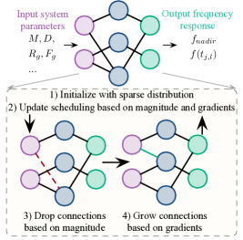
Figure 2: Sparse neural network training by leveraging the weight magnitude and gradient information.

III-B2a Sparse Distributing

We define sparsity $s^{l}\in(0,1)$ as the dropping fraction of the $l^{th}$ layer. The first layer is set as the dense layer, and the other layers are set as the sparse layers with predefined $s^{l}$ for the $l^{th}$ layer sparse training in a uniform way.

III-B2b Update Scheduling

The update scheduling drops a fraction of connections based on NN parameter magnitude and activates new ones based on NN parameter gradient magnitude iteratively at $\Delta T$ interval. So the updating fraction function by considering decaying is defined in Eq. eq: frac up.

$$\begin{aligned} f_{decay}(t;\alpha,T_{end})=\frac{\alpha}{2}(1+\cos\frac{t\pi}{T_{end}})\end{aligned}$$ (17)

where $T_{end}$ is the number of iteration for sparse training, and $\alpha$ is the initial drop fraction.

III-B2c Connection Dropping

In connection dropping of the $l^{th}$ layer, we utilize $ArgTopK(v,k)$ algorithm to select the top-$k$ maximum element indices of vector $v$ and drop the connection by $ArgTopK(-|\theta^{l}|,f_{decay}(t;\alpha,T_{end})(1-s^{l})N^{l})$.

III-B2d Connection Activating

After dropping, we further re-activate $k$ connections with the top-$k$ high magnitude gradients by $ArgTopK(\nabla_{\theta^{l}}L^{com}_{t},f_{decay}(t;\alpha,T_{end})(1-s^{l})N^{l})$. Newly activated connections are initialized as zero to avoid influencing the network output.

Remark 1.

The effect of gradients on the model’s training lies in the following two aspects: i) the gradients from the loss function can learn the prediction models by minimizing the proposed conservative loss function (stochastic gradient training); ii) they can also be utilized to grow necessary connection in the sparse neural networks to improve accuracy.

III-B3 Conservative Sparse SGD Algorithm

Based on the conservative loss of Eq. eq: com loss and sparse training designs, we propose the conservative sparse stochastic gradient descent (CS-SGD) algorithm for training the CSNN in algorithm 1.

1:  Input: Initialize the frequency dynamics model: $f_{\theta}$, dataset: $D=\{x_{i},y_{i}\}$, sparse distributing: $\mathbb{S}=\{s^{1},..,s^{L}\}$, updating scheduling parameters: $\Delta T$, $T_{end}$, $\alpha$, $f_{decay}$;

2:  Output: Trained frequency dynamics model $f_{\theta}$.

3:  for $t=1,...,T$ do

4:     Conservative Formulating:

5:     Calculate conservative loss $L^{com}_{t}=\sum L^{com}(f_{\theta}(x_{i}),y_{i})$ based on Eq. eq: conservative loss;

6:     Sparse Training:

7:     if $t\bmod\Delta T==0$ and $t\leq T_{end}$ then

8:        for $l=1,...,L$ do

9:           Calculate dropping and activating number $k=f_{decay}(t;\alpha,T_{end})(1-s^{l})N^{l}$;

10:           Drop connections based on $ArgTopK(-|\theta^{l}|,k)$;

11:           Activate connections based on $ArgTopK(\nabla_{\theta^{l}}L^{com}_{t},k)$;

12:        end for

13:     else

14:        Update CSNN parameters: $\theta\leftarrow\theta-\alpha\Delta_{\theta}L^{com}_{t}$;

15:     end if

16:  end for

Algorithm 1 Conservative Sparse Stochastic Gradient Descent Training Algorithm.

The key novelty of the proposed CS-SGD algorithm lies in incorporating the conservative loss function of Eq. eq: conservative loss and sparse training process with dropping and growing to train CSNN with conservativeness and sparsity for approximating the power system frequency dynamics. The weights and bias of trained CSNN are leveraged to formulate the equivalent mixed-integer linear frequency constraints, which can secure the system frequency stability. The conservativeness of CSNN guarantees safety of the transformed frequency constraints, and the sparsity of CSNN improving solution efficiency of the data-enhanced frequency constrained unit commitment optimization model with fewer optimizing variables.

III-C NN Embedded Frequency Constraints Transformation

After training, the proposed CSNN can be transformed into a series of mixed linear integer constraints using the big-M method. Based on Ref. [27], this paper formulates the general form of an $L$-layer feedforward neural network with ReLU as the activation function in Eq. eq: nn form, which is composed of stacked linear transformation (18a) and ReLU activation (18b).

Neural Network: $$v^{l}_{i}=\text{ReLU}(\theta^{l}_{i0}+\sum_{j\in\mathcal{N}^{l-1}}\theta^{l}_{ij}v^{l-1}_{j})$$ (18a)

where $$y=v^{L}=\theta^{L}_{0}+\sum_{j\in\mathcal{N}^{L-1}}\theta^{L}_{j}v^{L-1}_{j}$$ (18b)

where $v^{l}_{i}$ is the output of neuron $i$ in layer $l$ in a neuron network, $\theta^{l}_{ij}$ is the weight between neuron $i$ and $j$, and $\theta^{l}_{i0}$ is the bias of neuron $i$ in layer $l$.

For each layer of Eq. eq: nn form a, the ReLU operator, $\text{ReLU}(x)=\max\{0,x\}$, can be encoded using linear constraints in a big-M way from Ref. [22], as follows:

$$v \geq x,$$ (19a)

$$v \leq x-M_{L}(1-t),$$ (19b)

$$v \leq M_{U}t,$$ (19c)

$$v \geq 0,$$ (19d)

$$t \in\{0,1\}$$ (19e)

where $M_{U}$ and $M_{L}$ are positive and negative large value to relax the ReLU function.

III-D Data Processing Techniques

This part utilizes the data sampling strategy based on the boundary and Latin hypercube sampling to enhance the data quality for the predictive models. It constructs the stability region based on the convex hulls to prevent the extrapolating of predictive models.

III-D1 Data Sampling Strategy

The predictive model performance relies on the training dataset quality; thus, the data distribution is critical for constraint learning. The sampled data should be space-filling sufficiently to capture the frequency dynamics of frequency constraints in Eq. eq: freq conser. Inspired by Ref. [25], we utilize the boundary sampling and optimal Latin hypercube (OLH) sampling for constructing training set $\mathcal{Z}=\{M_{n},D_{n},R_{g,n},F_{g,n}\}_{n=1}^{N}$. In the process, the boundary sampling collects the corners of the $\mathcal{Z}$ hypercube by the input data bounds, and then we conduct the OLH sampling over the above hypercube. The detailed sampling procedures are illustrated in Ref. [25].

III-D2 Convex Hulls as Stability Region

The optimal solutions of mixed-integer linear programs are often located at the extremes of their feasible polyhedron region, which may harm the validity of the trained ML models. According to Ref. [22], the accuracy of an ML-based predictive model will deteriorate for points far away from the training dataset. So we construct stability regions to prevent the predictive model from extrapolating by the convex hull from the training dataset. For the training dataset $\mathcal{Z}$, we construct the following convex hull $CH(\mathcal{Z})$ in Eq. eq: ch z as the stability region.

$$\begin{gathered}CH(\mathcal{Z})=\big{\{}z|\sum_{i\in\mathcal{I}}\lambda_{i}\hat{z}_{i}=z,\sum_{i\in\mathcal{I}}\lambda_{i}=1,\lambda\geq 0\big{\}}\end{gathered}$$ (21)

However, there are two issues arising from the direct single convex hull. One issue is that the computing of the convex hull is exponential to data number in time and space; the other is that the data distribution in a single convex hull is not uniform. Some points cannot satisfy the requirement of system stability in Eq. eq: analytical transfer, and the single convex hull may include and extrapolate some infeasible points. So we propose the cluster-then-build strategy, which first clusters the trained dataset, builds a convex hull for each cluster, and unions them $\bigcup_{k\in\mathcal{K}}CH_{k}(\mathcal{Z})$ for preventing extrapolating in Eq. eq: K ch z.

$$\begin{aligned} \bigcup_{k\in\mathcal{K}}CH_{k}(\mathcal{Z})=\big{\{}z|\sum_{i\in\mathcal{I_{k}}}\lambda_{i}\hat{z}_{i}=z,\sum_{i\in\mathcal{I}}\lambda_{i}=u_{k},\sum_{k\in\mathcal{K}}u_{k}=1\\ \lambda\geq 0,\forall k,u\in\{0,1\}\big{\}}\end{aligned}$$ (22)

III-D3 Discussion

It should be noted that we need to construct and build different CSNN models and stability regions for different system and DER settings. Because the training of CSNNs is based on the sampled dataset from the system model with corresponding DER setting via Eq. eq: time domain and Eq. eq: f nadir. Different system and DER settings will affect the sampled dataset directly and further affect the training of CSNNs indirectly, leading to inaccurate approximation. Stability region is also constructed from the sampled dataset. So we need to retrain different learning models and construct different stability region for these circumstances, such as different DER settings, to improve approximation accuracy.

IV Data-enhanced Frequency-Constrained Unit Commitment with DER

Based on the above proposed CSNN, this section proposes the data-enhanced frequency constrained unit commitment (FCUC) with the converter-based DER. It firstly introduces the overall OCL framework for the proposed data-enhanced FCUC, then presents the conventional unit commitment model, and includes the data-enhanced frequency constraints to formulate the final data-enhanced model.

IV-A Overall Framework

Based on the CSNN and NN embedded transformation of section III, we propose the OCL framework for the data-enhanced FCUC with converter-based DERs, composed of the learning and optimization stages, as shown in Fig. 3. Its main idea lies in leveraging CSNN and the frequency data to enhance the power system decision-making and advance the data-driven integration modeling technique. The learning stage samples the stable instances from the frequency analytical expression of Eq. eq: f nadir and Eq. eq: freq stepwise, feeds them to training the CSNNs, constructs the stability region using the convex hulls for the stable instances, and evaluates their performance; the optimization stage embeds the stability region constraints of Eq. eq: K ch z and transformed CSNN constraints of Eq. eq: big-m in the system scheduling model to formulate the final data-enhanced FCUC model. It should be noted that: 1) the stability region and the CSNNs are constructed from the sampled dataset in different ways and are integrated into the conventional unit commitment model as mixed-integer linear constraints, so the stability region construction will not affect the training process of CSNNs; 2) DERs refer to the distributed photovoltaic (PV) and wind power (WP) generators concretely in this paper.

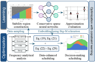
Figure 3: The optimization with constraint learning framework for the data-enhanced FCUC with DER.

IV-B Unit Commitment Considering Joint Reserve and Regulation Capacity

Based on the above OCL framework, we formulate the conventional unit commitment model considering joint reserve and regulation capacity to minimize the system operating cost under a series of operational constraints.

IV-B1 Model Objective

The objective of conventional unit commitment is to minimize the total system operating cost, which is composed of the operating cost $C_{oper}$, reserve cost $C_{rsv}$, and load shedding cost $C_{load}$ in Eq. eq: uc obj.

$$\min\quad C_{total}=C_{oper}+C_{rsv}+C_{load}$$ (23a)

$$C_{oper}=\sum_{t\in\mathcal{N}_{T}}\sum_{g\in\mathcal{N}_{G}}(C^{SU}_{g}x^{SU}_{g,t}+C^{SD}_{g}x^{SD}_{g,t}+f_{g}(p_{g,t}))$$ (23b)

$$C_{rsv}=\sum_{t\in\mathcal{N}_{T}}\Big{(}\sum_{g\in\mathcal{G}}C^{R}_{g}R_{g,t}+\sum_{w\in\mathcal{W}}C^{R}_{w}R_{w,t}+\sum_{pv\in\mathcal{PV}}C^{R}_{pv}R_{pv,t}\Big{)}$$ (23c)

$$C_{load}=\sum_{t\in\mathcal{N}_{T}}\sum_{n\in\mathcal{N}_{N}}\lambda_{L}p^{cur}_{n,t}$$ (23d)

where $C_{oper}$ includes the start-up, shut-down, and the fuel costs; $C_{rsv}$ includes the costs of the reserve from synchronous generators and converter-based PV/WP generators; $C_{load}$ includes the load shedding costs from different buses. The unit cost function $f_{g}(\cdot)$ can be piece-wised by SOS2 constraints.

IV-B2 Power Network Constraints

The node power balance equation and transmission power limited are formulated based on DC power flow model in Eq. eq: uc pnc.

$$\sum_{g\in\mathcal{G}_{n}}p_{g,t}+\sum_{w\in\mathcal{W}_{n}}p_{w,t}+\sum_{pv\in\mathcal{PV}_{n}}p_{pv,t}$$

$$+\sum_{m:(n,m)}B_{nm}(\delta_{nt}-\delta_{mt})=p^{D}_{n,t}-p^{cur}_{n,t}\quad\forall n,t$$ (24a)

$$|B_{nm}(\delta_{nt}-\delta_{mt})|\leq F^{max}_{nm}\quad\forall(n,m)\in\mathcal{L},\forall t$$ (24b)

where Eq. eq: uc pnc a enforces the bus power balance for each period, and Eq. eq: uc pnc b restricts the branch power flow under the given capacity.

IV-B3 Thermal Generator Operational Constraints

The ramping and power output restriction are formulated via MILP in Eq. eq: uc opera.

$$x_{g,t}p^{min}_{g}\leq p_{g,t}\leq x_{g,t}p^{max}_{g}\quad\forall g,t$$ (25a)

$$x^{SU}_{g,t}-x^{SD}_{g,t}=x_{g,t}-x_{g,t-1}\quad\forall g,t$$ (25b)

$$p_{g,t}-p_{g,t-1}\leq x_{g,t-1}Ru_{g}\quad\forall g,t$$ (25c)

$$p_{g,t-1}-p_{g,t}\leq x_{g,t}Rd_{g}\quad\forall g,t$$ (25d)

where Eq. eq: uc opera a restricts the generator power output; Eq. eq: uc opera b enforces the relationship between the on/off variables and start-up/shut-down variables; Eq. eq: uc opera c and Eq. eq: uc opera d restricts the generator ramping capacity.

IV-B4 Renewable Energy Generation Constraints

The actual power outputs of renewable energy generation are limited below the predicted values.

$$0 \leq p_{w,t}\leq\hat{p}_{w,t}\quad\forall w,t$$ (26a)

$$0 \leq p_{pv,t}\leq\hat{p}_{pv,t}\quad\forall pv,t$$ (26b)

where Eq. eq: uc res a and Eq. eq: uc res b restrict the actual power output of wind and PV below the day ahead predicted value.

IV-B5 System Reserve Constraints

The system reserve is restricted to cover the prediction errors of the DERs and load as follows:

$$\allowdisplaybreaks\begin{aligned} &\sum_{g\in\mathcal{G}}x_{g,t}P^{max}_{g}+\sum_{w\in\mathcal{W}}\hat{p}_{w,t}+\sum_{pv\in\mathcal{PV}}\hat{p}_{pv,t}+\sum_{n\in\mathcal{N}}p^{cur}_{n,t}\\ &\geq(1+\epsilon_{l})\sum_{n\in\mathcal{N}}\hat{p}^{D}_{n,t}\\ &+(1+\epsilon_{der})\big{(}\sum_{w\in\mathcal{W}}\hat{p}_{w,t}+\sum_{pv\in\mathcal{PV}}\hat{p}_{pv,t}\big{)}\quad\forall t.\end{aligned}$$ (27)

Eq. eq: uc rsv guarantees that the online generation capacity can satisfy the load demand with prediction errors, according to Ref. [10].

IV-C Data-enhanced Frequency Constraints

As discussed in section III, we propose the CSNN to approximate the nonlinear constraints of frequency nadir and stepwise constraints in a conservative way. So this part adds the CSNN embedded frequency dynamics constraints in Eq. eq: uc freq dyn and corresponding emergency regulation constraints in Eq. eq: uc em rsv into the above conventional unit commitment models for ensuring the frequency dynamics stability.

IV-C1 Inertia Parameter Aggregation

The system inertia variables $M$, $D$, $R_{g}$, and $F_{g}$ for Eq. eq: freq conser can be calculated by aggregating generators’ and PV/WP converters’ related parameters in Eq. eq: inertia agg.

$$M_{g}=\frac{\sum_{i\in\mathcal{N}_{g}}u_{gi}M_{gi}P_{gi}}{P^{b}_{g}},D_{g}=\frac{\sum_{i\in\mathcal{N}_{g}}u_{gi}D_{gi}P_{gi}}{P^{b}_{g}}$$ (28a)

$$F_{g}=\sum_{i\in\mathcal{N}_{g}}\frac{u_{gi}K_{gi}F_{gi}}{R_{gi}}\frac{P_{gi}}{P^{b}_{g}},R_{g}=\sum_{i\in\mathcal{N}_{g}}\frac{u_{gi}K_{gi}}{R_{gi}}\frac{P_{gi}}{P^{b}_{g}}$$ (28b)

$$R_{d}=\sum_{j\in\mathcal{N}_{d}}\frac{u_{dj}K_{dj}}{R_{dj}}\frac{P_{dj}}{P^{b}_{der}}$$ (28c)

$$M_{d}=\sum_{k\in\mathcal{N}_{v}}u_{dk}M_{dk}\frac{P_{dk}}{P^{b}_{der}},D_{d}=\sum_{k\in\mathcal{N}_{v}}u_{dk}D_{dk}\frac{P_{dk}}{P^{b}_{der}}$$ (28d)

$$M=\frac{M_{g}P^{b}_{g}+M_{der}P^{b}_{der}}{P^{b}_{g}+P^{b}_{der}}$$ (28e)

$$D=\frac{D_{g}P^{b}_{g}+D_{der}P^{b}_{der}+R_{d}P^{b}_{der}}{P^{b}_{g}+P^{b}_{der}}.$$ (28f)

IV-C2 Frequency Dynamics Constraints

The proposed CSNN is utilized to reach the convex lower bounds of nonlinear frequency constraints by transforming $f_{nadir}$ and $f(t_{j,l})$ into $\hat{f}^{csnn}_{nadir}$ and $\hat{f}^{csnn}(t_{j,l})$ in Eq. eq: nadir contrs and Eq. eq: freq stepwise trans, as follows:

$$\hat{f}^{csnn}_{nadir}(M,D,R_{g},F_{g})\geq f_{min}$$ (29a)

$$\hat{f}^{csnn}(M,D,R_{g},F_{g};t_{j,l})\geq f_{lim}(t_{j,l}).$$ (29b)

where $\hat{f}^{csnn}_{nadir}$ and $\hat{f}^{csnn}(t_{j,l})$ can be transformed into mixed-integer linear constraints via Eq. eq: big-m. Taking Eq. eq: uc freq dyn a as an example, its equivalent mixed-integer constraints is formulated and incorporated by taking $x=(M,D,R_{g},F_{g})$ in Eq. eq: freq milp.

$$v^{1}_{i}=\theta^{1}_{i0}+\sum_{j\in\mathcal{X}}\theta^{l}_{ij}x_{j}, i\in[N_{1}]$$ (30a)

$$\hat{v}^{l}_{i}=\theta^{l}_{i0}+\sum_{j\in\mathcal{N}^{l-1}}\theta^{l}_{ij}v^{l-1}_{j}, l\in[L],i\in[N_{l}]$$ (30b)

$${v}^{l}_{i}\geq\hat{v}^{l}_{i}, l\in[L],i\in[N_{l}]$$ (30c)

$${v}^{l}_{i}\leq\hat{v}^{l}_{i}-M^{L}_{l,i}(1-t_{l,i}), l\in[L],i\in[N_{l}]$$ (30d)

$${v}^{l}_{i}\leq M^{H}_{l,i}t_{l,i}, l\in[L],i\in[N_{l}]$$ (30e)

$${v}^{l}_{i}\geq 0,\quad t_{l,i}\in\{0,1\}, l\in[L],i\in[N_{l}]$$ (30f)

$$\hat{f}^{csnn}_{nadir,m}=\theta^{L}_{i0}+\sum_{j\in\mathcal{N}^{L-1}}\theta^{L}_{ij}v^{L-1}_{j} m\in[N_{M}],i\in[N_{L}]$$ (30g)

where $[N_{l}]$ is the set of input neurons in layer $l$, and $[L]$ is the set of output neurons in layer $l$.

IV-C3 Emergency Regulation Formulation

Eq. eq: uc em rsv provides the headroom regulation capacity for the primary frequency response from synchronous and converter-based generators.

$$R_{g,t}=p^{max}_{g}-p_{g,t}\geq u_{g,t}\frac{K_{g}}{R_{g}}p^{max}_{g}\gamma(f_{0}-f_{min})$$ (31a)

$$R_{w,t}=\hat{p}^{w,t}-p_{w,t}\geq u_{w,t}\frac{1}{R_{w}}\hat{p}^{w,t}\gamma(f_{0}-f_{min})$$ (31b)

$$R_{pv,t}=\hat{p}^{pv,t}-p_{pv,t}\geq u_{pv,t}\frac{1}{R_{pv}}\hat{p}^{pv,t}\gamma(f_{0}-f_{min})$$ (31c)

$$\forall g\in\mathcal{G},w\in\mathcal{W},pv\in\mathcal{PV},\quad\forall t.$$

The largest frequency deviation ($f_{0}-f_{min}$) is larger the quasi-steady state frequency deviation. According to Ref. [10], the $\gamma$ is set as 0.5 for emergency reserve capacity.

So the combination of unit commitment modeling and data-enhanced frequency constraints constructs the final data-enhanced FCUC with converter-based DER considering both the system reserve for uncertainty and the regulation capacity for emergency, which follows the mixed-integer linear programming form and can be solved by the off-the-shelf solvers efficiently.

V Case Study

In the case study, the modified IEEE 118-bus and 1888-bus systems with multiple PV and WP is utilized to verify the effectiveness and efficiency of the data-enhanced frequency constrained unit commitment model with converter-based DER. The proposed model is composed of the learning and optimization stages. So we construct the learning models with the Pytorch package and the optimization models with the Cvxpy package equipped by the Gurobi solver. All the experiments are implemented in a MacbookPro laptop with RAM of 16 GB, CPU Intel Core I7 (2.6 GHz). The other detailed system parameter setting of the modified system is attached in Ref. [34] and Ref. [35].

V-A Data Preparation and Experiment Setting

This part mainly prepares the essential data and problem settings in the OCL framework for the data-enhanced FCUC model of Fig. 3, including 1) the neural network parameter setting of the learning stage 2) and the inertia parameter setting of the optimization stage.

V-A1 Learning Stage

In the learning stage, we first generate 10000 feasible samples based on the system frequency dynamics of Eq. eq: time domain and Eq. eq: f nadir to construct the training dataset for the stability region and learning model training. Then the proposed CSNNs take the system inertia parameter $x=(M,D,R_{g},F_{g})$ as the feature vector, and the input feature vector is normalized into the scale of 0-1 for model training based on their maximum value. We compare the proposed conservative sparse neural network (CSNN) with the conservative neural network (C-NN) and the conventional neural network (NN) under the same initial parameters of full connected neural networks in Tab. I. The hyperparameter configuration in Tab. I is determined based on the hyperparameter tuning with the high approximation accuracy of learning models. The change of these hyperparameter values does not enhance the approximation accuracy of the learning models in our cases.

TABLE I: The parameters of neural network models.

Hyperparameter	Value	Hyperparameter	Value
Optimizer	Adam	Learning rate	1e-6
Hidden layers	[100, 100]	Batch size	32
Activation function	ReLU	Dropout	0.2

We clarify the relationship among CSNN, C-NN, and NN, where C-NN further utilizes the conservative loss of Eq. eq: conservative loss compared to NN, and CSNN further employs the sparse training of algorithm 1 compared to C-NN. The same hyperparameters of Tab. I are utilized to initialize the CSNN, C-NN, and NN to avoid the hyperparameter effect on model comparison of different neural networks.

V-A2 Optimization Stage

In the optimization stage, we prepare the inertia parameters of different generators and VSM/droop control parameters of PV and wind power converters from Ref. [15], as illustrated in Tab. II. The frequency nadir, stepwise frequency, and QSS requirement are set based on the ENTSO-E standard [32] and Ref. [8].

TABLE II: The parameters of different generator and control methods.

Type	$M_{gi}$	$K_{gi}$	$F_{gi}$	$R_{ci}$	$D_{ci}$
Nuclear	9s	0.98	0.25	0.04	0.6
CCGT	14s	1.1	0.15	0.01	0.6
OCGT	11s	0.95	0.35	0.03	0.6
Converter / VSM	12s	1.0	-	-	0.6
Converter / Droop	-	1.0	-	0.05	-

V-B Frequency Approximation Performance Evaluation

This part firstly analyzes the approximation performance of the proposed CSNN in describing the frequency dynamics. It then verifies its effectiveness in the data-enhanced frequency constrained model with the stability region design.

V-B1 CSNN Analysis

V-B1a Training Process

Fig. 4 compares CSNN, C-NN, and NN training processes for the frequency nadir and stepwise relationship approximation. In the training process, NN achieves a lower approximation error than CSNN and C-NN due to the consideration of the conservative loss function, and CSNN exhibits a little lower error than C-NN thanks to the sparse designs.

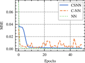
(a) Training process of the frequency nadir.

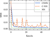
(b) Training process of the stepwise frequency constraints.

Figure 4: The training process of frequency nadir and stepwise frequency constraint learning.

V-B1b Approximation Error

We further compare the detailed approximation performance of CSNN with C-NN and NN. Fig. 5 demonstrates the approximation error distribution of the above four models by the boxen plot.

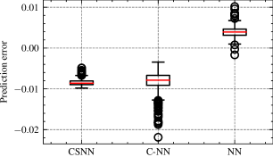
Figure 5: The approximation errors of different models in boxen plot.

As shown in Fig. 5, the approximation errors of NN are located around zero with negative and positive values, and in contrast, the approximation errors of CSNN and C-NN are located below zero with only negative values, demonstrating their conservativeness. The median error of NN is above zero. CSNN exhibits a more accurate approximation with a more concentrated error distribution than C-NN.

We utilize the mean square error (MSE), mean absolute percentage error (MAPE) metrics in Eq. eq: mse mape, and negative rate to measure the approximation performance numerically.

$$\begin{aligned} \mathcal{L}_{MSE}=\frac{1}{N}\sum_{i}^{N}(f_{i}-\hat{f}_{i})^{2},\quad\mathcal{L}_{MAPE}=\frac{1}{N}\sum_{i}^{N}|\frac{f_{i}-\hat{f}_{i}}{f_{i}}|.\end{aligned}$$ (32)

As illustrated in Tab. III, for MAPE, CSNN achieves 0.87% lower MAPE than NN, 0.76% lower MAPE than C-NN, and 0.11% lower MAPE than PWL; for MSE, CSNN increases 142.14% MSE of NN but decrease 91.35% MSE of C-NN and 74.85% MSE of C-NN, which sacrifices some approximation accuracy to guarantee conservativeness. As for the negative rate, both CSNN and C-NN exhibit a 100% negative rate, demonstrating the effectiveness of the conservative loss design. In contrast, the negative rate of NN is only 85.43%, which may result in the frequency requirement violation.

TABLE III: Approximation error comparison of different methods.

Models	CSNN	C-NN	NN	PWL
MAPE	0.23%	1.10%	0.99%	0.44%
MSE	$7.584e^{-5}$	$8.772e^{-4}$	$3.132e^{-5}$	$3.015e^{-4}$
Negativeness	100%	100%	85.43%	65.46%

We note that 1) the negativeness denotes the ratio of the negative error instance number to the total number; 2) PWL denotes the conventional piece-wise linear approximation.

V-B1c Sparsity Comparison

To verify the sparsity of CSNN, we compare the non-zero parameter number of the above four models, where lower parameters mean a higher sparsity.

TABLE IV: The parameter number of different methods for frequency nadir.

Models	CSNN	C-NN	NN
Number	1395	10701	10701
Sparsity rate	86.96%	0%	0%

We note that the sparsity rate denotes the ratio of the parameter reduction number to the total parameter number.

For the frequency nadir constraint learning of Eq. eq: freq conser a in Tab. IV, the corresponding CSNN has only 1395 parameters and achieves the 86.96% reduction of the dense neural networks of C-NN and NN, verifying the effectiveness of sparse training.

TABLE V: The parameter number of different methods for stepwise constraints.

Models	CSNN	C-NN	NN
Number	1442	10903	10903
Sparsity rate	86.77%	0%	0%

For the stepwise frequency constraint learning of Eq. eq: freq conser b in Tab. V, the corresponding CSNN has only 1442 parameters and achieves the 86.77% reduction of the dense neural networks of C-NN and NN.

V-C Comparison of Optimization Scenarios

In this part, we first compare the operational performance of the data-enhanced frequency constrained unit commitment model and then verify the efficacy of the sparse design of neural networks, stability region, and the stepwise frequency constraints.

V-C1 Operation Performance

We further compare the data-enhanced FCUC with DER to the conventional unit commitment for verifying the necessity of frequency constraints and the effectiveness of DER participation.

V-C1a Results

Tab. VI compares the operational costs and renewable abandoned rates of the scheduling model with/without frequency constraints.

TABLE VI: Operational comparison of different models in the modified 118-bus system.

Models	Cost / $	Abandoned Rate	Violation Rate
Conventional UC	$19.65e^{5}$	0.00%	100%
Data-enhanced FCUC	$21.27e^{5}$	2.64%	0%

We note that the abandoned rate denotes the ratio of the abandoned renewable power to the total renewable generation.

The data-enhanced FCUC increases the operational cost by 8.24% and the renewable abandoned rate by 2.64% but decreases the system frequency violation rate from 100% to 0% under large contingency, verifying the effectiveness of the proposed model. The increase of abandoned renewable supports system inertia. Through the frequency constraints, the system will enhance the system inertia and frequency response by increasing the online units and exploiting the frequency support from DER, leading to a higher operational cost, abandoned rate, and more stable system operation.

Fig. 6 further compares the operational unit status between the convention scheduling and frequency-constrained scheduling, demonstrating that the frequency constraints enforce the unit start-up to guarantee the system stability.

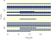
(a) Conventional scheduling.

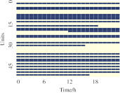
(b) Frequency-constrained scheduling

Figure 6: The unit status under different scheduling scenarios in the modified 118-bus system.

V-C1b Dynamics Analysis

We simulate the frequency dynamics under the scheduling models with and without frequency constraints under the 500 MW power loss contingency in Fig. 7, verifying their effectiveness.

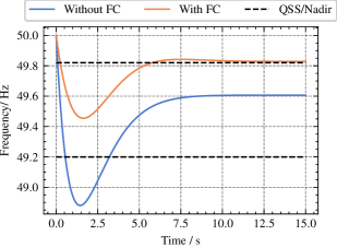
Figure 7: Frequency dynamics comparison in the modified 118-bus system.

As shown in Fig. 7, the orange line of dynamics under FCUC satisfies the frequency nadir, stepwise, and QSS requirements compared to the blue line under the conventional scheduling.

V-C2 Benefits of Sparse Neural Networks

Compared with the piece-wise linear regression, the high representational capacity of sparse neural networks will help capture the relationship between frequency dynamics and inertia parameters in a more optimization-efficient way.

TABLE VII: Comparison of different frequency models in the modified 118-bus system.

Models	CSNN	C-NN	NN
Solving time/min	7.12	122.65	153.55

Tab. VII compares the solving time and costs of the data-enhanced FCUC integrated with different neural networks. The solving time under CSNN is 17.23 times faster than C-NN and 21.57 times faster than NN, verifying the solution acceleration effectiveness of sparsity design.

V-C3 Benefits of Stability Region

We should guarantee the performance of the data-driven method design because robustness matters more than optimality. So we construct the clustered convex hulls from the data to build the stability region adding to the optimization models. The below Fig. 8 shows the area of infeasible points and the convex hulls of clustered feasible points.

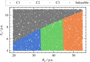
Figure 8: Analysis of convex hulls as stability region.

V-D Scalability and Comparison Analysis

For the generality of the proposed data-enhanced FCUC, we further discuss the scalability of the proposed framework via the modified 1888-bus system experiments based on Ref. [35] and verify the effectiveness and efficiency of the proposed CSNN via the comparison the state-of-the-art machine learning algorithms [36, 37, 38].

V-D1 Scalability Analysis

We apply the data-enhanced FCUC model in a modified 1888-bus system to verify the scalability of the proposed method that the proposed data-enhanced FCUC increases 3.6% operational cost and 4.23% renewable abandoned rate to achieve the 0% frequency violation rate under contingency and ensure system stable operation, as shown in the following Tab. VIII.

TABLE VIII: Operational comparison of different models in the modified 1888-bus system.

Models	Cost / $	Abandoned Rate	Violation Rate
Conventional UC	$1.469e^{7}$	0%	100%
Data-enhanced FCUC	$1.524e^{7}$	4.23%	0%

V-D2 Comparison Analysis

To verify the efficiency and effectiveness, we further compare the proposed CSNN model with other state-of-the-art machine learning models including the optimal regression trees (ORT) [36], random forest (RF) [37], and support vector regression (SVR) [38] models.

TABLE IX: Approximation error comparison of different ML models in the modified 1888-bus system.

Models	CSNN	ORT	RF	SVR
MAPE	0.23%	0.11%	0.32%	0.35%
MSE	$7.584e^{-5}$	$2.83e^{-5}$	$1.15e^{-4}$	$1.47e^{-4}$
Negativeness	100%	45.71%	55.07%	84.52%

We note that the negativeness denotes the ratio of the negative error instance number to the total number.

As shown in Tab. IX, though the prediction accuracy of CSNN is lower than ORT but higher than RL and SVR, the proposed CSNN achieve 100% negative rate compared to ORT, RF, and SVR, verifying its prediction conservativeness.

To summarize, our proposed data-enhanced FCUC model exhibits scalability for various testing systems and effectiveness for approximation conservativeness compared to various ML models.

VI Conclusion

Faced with the complex frequency dynamics under the high penetration of the converter-based DER, this paper proposes to learn the frequency dynamics by CSNN and incorporate CSNN into the system optimization to facilitate system reliable operation, composed of learning and optimization stages. In the learning stage, the proposed CSNN can achieve the conservativeness against frequency violation and the sparsity for solving acceleration; in the optimization stage, the trained CSNNs are transformed into MILP constraints using the big-M method and embedded into the conventional UC model to establish the final data-enhanced FCUC model. The case study verifies 1) the effectiveness of the proposed model by achieving higher approximation accuracy, around 87% fewer parameters, and 21.57 times faster solving speed compared to that of the conventional NN in the modified 118-bus system; 2) the stable system operation against the frequency requirement violation under contingency. The proposed data-enhanced FCUC model leverages and incorporates the CSNN to manage the system inertia with DERs effectively and boost the system reliability.

Linwei Sang (S’20) received the M.S. degree from the School of Electric Engineering, Southeast University, Nanjing, China in 2021. He is currently pursuing the Ph.D. degree in the Tsinghua-Berkeley Shenzhen Institute, Tsinghua University, Shenzhen, China. His research includes the integration of machine learning and optimization in smart grid, the control of the distributed energy, and demand side resource management.

Yinliang Xu (SM’19) received the B.S. and M.S. degrees in control science and engineering from the Harbin Institute of Technology, Harbin, China, in 2007 and 2009, respectively, and the Ph.D. degree in electrical and computer engineering from New Mexico State University, Las Cruces, NM, USA, in 2013. He is currently an Associate Professor with Tsinghua-Berkeley Shenzhen Institute, Tsinghua Shenzhen International Graduate School, Tsinghua University, Beijing, China. His research interests include distributed control and optimization of power systems, renewable energy integration, and microgrid modeling and control.

Zhongkai Yi (Member, IEEE) received the B.S. and M.S. degrees in Electrical Engineering from Harbin Institute of Technology in 2016 and 2018, respectively, and the Ph.D. degree in Electrical Engineering from Tsinghua University in Jan. 2022. He is currently an associate professor with the Department of Electrical Engineering, Harbin Institute of Technology. From January 2022 to April 2023, He is an algorithm expert with the Machine Intelligence Research Sector, Alibaba DAMO Academy. His research interests include the optimization and machine learning in power systems.

Lun Yang received the Ph.D. degree in Electrical Engineering from Tsinghua University, Beijing, China, in October, 2022. He is currently an Assistant Professor in the School of Automation Science and Engineering of Xi’an Jiaotong University. Before that, he was a visiting scholar with The Chinese University of Hong Kong, Shenzhen, from October 2022 to April 2023. His research interests include power and energy systems operations and data-driven optimization under uncertainty. He was the recipient of the best paper award at 2020 IEEE PES General Meeting.

Huan Long (M’15) received the B.Eng. degree from Huazhong University of Science and Technology, Wuhan, China, in 2013, and the Ph.D. degree from the City University of Hong Kong, Hong Kong, in 2017. She is currently an Associate Professor with the School of Electrical Engineering, Southeast University, Nanjing, China. Her research fields include artificial intelligence applied in modeling, optimizing, monitoring the renewable energy system and power system.

Hongbin Sun (Fellow, IEEE) received his double B.S. degrees from Tsinghua University in 1992, the Ph.D. from Dept. of E.E., Tsinghua University in 1996. He is now ChangJiang Scholar Chair professor and the director of energy management and control research center, Tsinghua University. He also serves as the editor of the IEEE TSG, associate editor of IET RPG, and member of the Editorial Board of four international journals and several Chinese journals. His technical areas include electric power system operation and control with specific interests on the Energy Management System, Automatic Voltage Control, and Energy System Integration.

References

- [1] J. Chilvers, R. Bellamy, H. Pallett, and T. Hargreaves, “A systemic approach to mapping participation with low-carbon energy transitions,” Nat. Energy, vol. 6, no. 3, pp. 250–259, Mar. 2021.
- [2] F. Milano, F. Dörfler, G. Hug, D. J. Hill, and G. Verbič, “Foundations and challenges of low-inertia systems,” 2018 Power Systems Computation Conference (PSCC), 2018, pp. 1-25.
- [3] H. Cui et al., “Disturbance propagation in power grids with high converter penetration,” Proc. IEEE, early access, doi: 10.1109/JPROC.2022.3173813.
- [4] G. Delille, B. Francois and G. Malarange, “Dynamic frequency control support by energy storage to reduce the impact of wind and solar generation on isolated power system’s inertia,” IEEE Trans. Sustain. Energy, vol. 3, no. 4, pp. 931-939, Oct. 2012.
- [5] F. Teng, V. Trovato, and G. Strbac, “Stochastic scheduling with inertia-dependent fast frequency response requirements,” IEEE Trans. Power Syst., vol. 31, no. 2, pp. 1557-1566, Mar. 2016.
- [6] L. Badesa, F. Teng, and G. Strbac, “Simultaneous scheduling of multiple frequency services in stochastic unit commitment,” IEEE Trans. Power Syst., vol. 34, no. 5, pp. 3858-3868, Sept. 2019.
- [7] L. Badesa, F. Teng, and G. Strbac, “Optimal portfolio of distinct frequency response services in low-inertia systems,” IEEE Trans. Power Syst., vol. 35, no. 6, pp. 4459-4469, Nov. 2020.
- [8] J. Schipper, A. Wood and C. Edwards, “Optimizing instantaneous and ramping reserves with different response speeds for contingency—part I: methodology,” IEEE Trans. Power Syst., vol. 35, no. 5, pp. 3953-3960, Sept. 2020.
- [9] M. Paturet, U. Markovic, S. Delikaraoglou, E. Vrettos, P. Aristidou, and G. Hug, “Stochastic unit commitment in low-inertia grids,” IEEE Trans. Power Syst., vol. 35, no. 5, pp. 3448-3458, Sept. 2020.
- [10] Z. Zhang, E. Du, F. Teng, N. Zhang, and C. Kang, “Modeling frequency dynamics in unit commitment with a high share of renewable energy,” IEEE Trans. Power Syst., vol. 35, no. 6, pp. 4383-4395, Nov. 2020.
- [11] Z. Zhang, M. Zhou, Z. Wu, S. Liu, Z. Guo, and G. Li, “A frequency security constrained scheduling approach considering wind farm providing frequency support and reserve,” IEEE Trans. Sustain. Energy, vol. 13, no. 2, pp. 1086–1100, 2022.
- [12] Y. Yuan, Y. Zhang, J. Wang, Z. Liu and Z. Chen, “Enhanced frequency-constrained unit commitment considering variable-droop frequency control from converter-based generator,” IEEE Trans. Power Syst., early access, doi: 10.1109/TPWRS.2022.3170935.
- [13] X. Wang and F. Blaabjerg, “Harmonic stability in power electronic-based power systems: concept, modeling, and analysis,” IEEE Trans. Smart Grid, vol. 10, no. 3, pp. 2858-2870, May 2019.
- [14] R. Henriquez-Auba, J. D. Lara, D. S. Callaway and C. Barrows, “Transient simulations with a large penetration of converter-interfaced generation: scientific computing challenges and opportunities,” IEEE Electrif. Mag., vol. 9, no. 2, pp. 72-82, Jun. 2021.
- [15] U. Markovic, Z. Chu, P. Aristidou, and G. Hug, “LQR-based adaptive virtual synchronous machine for power systems With high inverter penetration,” IEEE Trans. Sustain. Energy, vol. 10, no. 3, pp. 1501-1512, Jul. 2019.
- [16] M. Chen, D. Zhou, A. Tayyebi, E. Prieto-Araujo, F. Dörfler and F. Blaabjerg, “Generalized multivariable grid-forming control design for power converters,” IEEE Trans. Smart Grid, vol. 13, no. 4, pp. 2873-2885, Jul. 2022.
- [17] W. Yan, L. Cheng, S. Yan, W. Gao, and D. W. Gao, “Enabling and evaluation of inertial control for PMSG-WTG using synchronverter with multiple virtual rotating masses in microgrid,” IEEE Trans. Sustain. Energy, vol. 11, no. 2, pp. 1078-1088, Apr. 2020.
- [18] R. Xia, Y. Chen, and B. Ren, “Improved anti-occlusion object tracking algorithm using Unscented Rauch-Tung-Striebel smoother and kernel correlation filter,” J. King Saud Univ. - Comput. Inf. Sci., vol. 34, no. 8, Part B, pp. 6008–6018, 2022.
- [19] J. Zhang, W. Feng, T. Yuan, J. Wang, and A. K. Sangaiah, “SCSTCF: Spatial-Channel Selection and Temporal Regularized Correlation Filters for visual tracking,” Appl. Soft Comput., vol. 118, p. 108485, 2022.
- [20] Y. Chen et al., “Image super-resolution reconstruction based on feature map attention mechanism,” Appl. Intell., vol. 51, no. 7, pp. 4367–4380, Jul. 2021.
- [21] J. Zhang, X. Zou, L. D. Kuang, J. Wang, R. S. Sherratt, X. Yu. “CCTSDB 2021: A more comprehensive traffic sign detection benchmark,” Hum.-centric Comput. Inf. Sci., vol. 12, no. 23, 2022.
- [22] D. Maragno, H. Wiberg, D. Bertsimas, S. I. Birbil, D. den Hertog, and A. Fajemisin, “Mixed-integer optimization with constraint learning,” arXiv, 2021, doi: https://arxiv.org/abs/2111.04469.
- [23] A. Fajemisin, D. Maragno, and D. den Hertog, “Optimization with constraint learning: a framework and survey,” arXiv, 2021, doi: https://arxiv.org/abs/2110.02121.
- [24] Y. Bengio, A. Lodi, and A. Prouvost, “Machine learning for combinatorial optimization: A methodological tour d’horizon,” Eur. J. Oper. Res., vol. 290, no. 2, pp. 405–421, 2021.
- [25] D. Bertsimas and B. Öztürk, “Global optimization via optimal decision trees,” arXiv, doi: https://arxiv.org/abs/2202.06017.
- [26] S. Sun, Z. Cao, H. Zhu, and J. Zhao, “A survey of optimization methods from a machine learning perspective,” IEEE Trans. Cybern., vol. 50, no. 8, pp. 3668-3681, Aug. 2020.
- [27] R. Anderson, J. Huchette, W. Ma, C. Tjandraatmadja, and J. P. Vielma, “Strong mixed-integer programming formulations for trained neural networks,” Math. Program., vol. 183, no. 1, pp. 3–39, Sep. 2020.
- [28] U. Evci, T. Gale, J. Menick, P. S. Castro, and E. Elsen, “Rigging the lottery: making all tickets winners,” Int. Conf. Mach. Learn., 2020, pp. 471–481.
- [29] J. Frankle and M. Carbin, “The lottery ticket hypothesis: finding sparse, trainable neural networks,” Int. Conf. Learn. Represent., New Orleans, LA, USA, May 2019.
- [30] P. S. Kundur, N. J. Balu, and M. G. Lauby, “Power system dynamics and stability,” Power System Stability and Control, vol. 3, 2017.
- [31] P. Daly, H. W. Qazi and D. Flynn,“RoCoF-constrained scheduling incorporating non-synchronous residential demand response,” IEEE Trans. Power Syst., vol. 34, no. 5, pp. 3372-3383, Sept. 2019.
- [32] ENTSO-E, “Frequency stability evaluation criteria for the synchronous zone of continental Europe,” ENTSO-E, Tech. Rep., 2016.
- [33] H. Ahmadi and H. Ghasemi, “Security-constrained unit commitment with linearized system frequency limit constraints,” IEEE Trans. Power Syst., vol. 29, no. 4, pp. 1536–1545, Jul. 2014.
- [34] https://github.com/sanglinwei/NN4UC_dataset
- [35] A. S. Xavier, A. M. Kazachkov, O. Yurdakul, F. Qiu. “UnitCommitment.jl: a Julia/JuMP optimization package for security-constrained unit commitment (version 0.22),” Zenodo, 2022. DOI: 10.5281/zenodo.4269874.
- [36] D. Bertsimas, J. Dunn, and Y. Wang, “Near-optimal nonlinear regression trees,” Oper. Res. Lett., vol. 49, no. 2, pp. 201–206, Mar. 2021.
- [37] H. Aprillia, H. -T. Yang and C. -M. Huang, “Statistical load forecasting using optimal quantile regression random forest and risk assessment index,” IEEE Trans. Smart Grid, vol. 12, no. 2, pp. 1467-1480, Mar. 2021.
- [38] J. Zhang, H. Jia and N. Zhang, “Alternate support vector machine decision trees for power systems rule extractions,” IEEE Trans. Power Syst., vol. 38, no. 1, pp. 980-983, Jan. 2023.