Realizing quantum optics in structured environments with giant atoms

Abstract

To go beyond quantum optics in free-space setups, atom-light interfaces with structured photonic environments are often employed to realize unconventional quantum electrodynamics (QED) phenomena. However, when employed as quantum buses, those long-distance nanostructures are limited by fabrication disorders. In this work, we alternatively propose to realize structured light-matter interactions by engineering multiple coupling points of hybrid giant atom-conventional environments without any periodic structure. We present a generic optimization method to obtain the real-space coupling sequence for multiple coupling points. We report a broadband chiral emission in a very wide frequency regime, with no analog in other quantum setups. Moreover, we show that the QED phenomena in the band gap environment, such as fractional atomic decay and dipole-dipole interactions mediated by a bound state, can be observed in our setup. Numerical results indicate that our proposal is robust against fabrication disorders of the coupling sequence. Our work opens up a new route for realizing unconventional light-matter interactions.

Introduction.—

Harnessing interactions between quantum emitters and quantized electromagnetic fields is a central topic of quantum optics Scully and Zubairy (1997); Agarwal (2012); Kimble et al. (1977); Cohen-Tannoudji et al. (1998); Gu et al. (2017); Kockum et al. (2019). In recent years, a burgeoning paradigm with giant atoms, which are coupled to waveguides at multiple separate points with their sizes comparable to photonic wavelengths, provides unanticipated opportunities to gain insights into exotic quantum optics beyond the dipole approximation Gustafsson et al. (2014); Kockum et al. (2014); Andersson et al. (2019); Zhao and Wang (2020); Guo et al. (2020a); Du et al. (2021); Soro and Kockum (2022); Yin et al. (2022); Du et al. (2022); Wang and Li (2022); Xiao et al. (2022); Cheng et al. (2022); Jia and Yu (2023); Santos and Bachelard (2023). The nonlocal coupling points cause nontrivial phases accumulation of the propagating field from a single giant emitter Kannan et al. (2020); Guo et al. (2017); Wang et al. (2021), allowing to observe exotic phenomena with no analog in small atom setups. The examples include decoherence-free interaction and oscillating bound states, which are caused by quantum interference and time-delay effects, respectively Kockum et al. (2018); Guo et al. (2020b); Lim et al. (2022).

Structured dielectric environments, which are scalable in integrated chips, have achieved tremendous progresses in quantum optics Lodahl et al. (2015); Goban et al. (2015); Roy et al. (2017); Chang et al. (2018); Yu et al. (2019); Scigliuzzo et al. (2022); Tang et al. (2022). Compared with free-space setups, the vacuum mode properties and dispersion relation can be tailored freely by shaping the dielectric structures Kofman et al. (1994); Smith et al. (2000); Lambropoulos et al. (2000); Kafesaki et al. (2007); Lu et al. (2014); Indrajeet et al. (2020); Stewart et al. (2020). One emblematic example is photonic crystal waveguides (PCWs), where the dielectric profile is periodically modulated, leading to the appearance of band gaps John and Wang (1990); Le Kien et al. (2004, 2005); Vetsch et al. (2010); Hung et al. (2013); Corzo et al. (2016); Liu and Houck (2017). Inside the gap, stable bound states of the hybrid photon and emitter are formed, which can alternatively mediate long-range interactions between emitters Zhou et al. (2008a); Liao et al. (2010); Goban et al. (2014); Douglas et al. (2015, 2016); Hood et al. (2016); González-Tudela et al. (2015); Munro et al. (2017); Leonforte et al. (2021). Moreover, when light is tightly transversely confined in high refractive-index materials, chiral emission occurs in nanophotonic structures owing to spin-momentum locking Mitsch et al. (2014); Bliokh et al. (2015a); Petersen et al. (2014); Young et al. (2015); Söllner et al. (2015); Bliokh et al. (2015b); Coles et al. (2016); Lodahl et al. (2017). However, fabricating long-distance nanostructures is very challenging when configuring those nanophotonic materials as quantum buses for quantum information processing Goban et al. (2014); Douglas et al. (2015). Due to unavoidable fabrication disorders and defects, photons are scattered repeatedly, and their fragile quantum coherence is destroyed Patterson et al. (2009); García et al. (2010); Lang et al. (2015); Mann et al. (2015).

In this work, we show that structured light-matter interactions can be alternatively realized by spatially designing a giant atom’s coupling sequence with a conventional photonic waveguide without any periodic structure. We present a generic optimization method to obtain real-space coupling sequences for any target momentum-space interaction. As examples, we show that both broadband chiral emission and band gaps effects can be realized by considering tens of coupling points in a conventional one-dimensional (1D) waveguide. Numerical results indicate that our proposal is robust against fabrication disorders in the coupling sequences, and can avoid localization and decoherence of photons appearing in long-distance nanostructures.

Optimizing coupling sequence.—

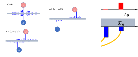
Figure 1: (a) Sketch of our proposal: A giant atom couples to a conventional 1D waveguide at positions $x_{1},...,x_{N}$. The coupling sequence $g(x_{i})=A(x_{i})e^{i\theta(x_{i})}$ is obtained via optimization methods sup .

The generic Hamiltonian of a quantum emitter interacting with a bosonic bath can be written as (setting $\hbar=1$)

$$H_{\mathrm{int}}=\sum_{k}{\Delta_{k}a_{k}^{\dagger}a_{k}}+\sum_{k}{G_{k}\left(a_{k}^{\dagger}\sigma_{-}+\mathrm{H}.\mathrm{c}.\right)},$$ (1)

where $\Delta_{k}=\omega_{k}-\omega_{q}$, with $\omega_{q}$ being the atomic transition frequency. Assuming a giant atom interacting with the waveguide at multiple points $X=\{x_{1},...,x_{N}\}$ (see Fig. 1), the $k$-space interaction is thus written as $G_{k}=\sum_{x_{i}}{g\left(x_{i}\right)e^{-ikx_{i}}}$, with $g(x_{i})=A(x_{i})e^{i\theta(x_{i})}$ being the interaction strength at $x_{i}$ (see Fig. 1). For small-atom setups, $G_{k}$ is approximately a constant due to the point-like coupling between the emitter and waveguide. Therefore, the structural engineering of the photonic waveguide’s dispersion relation $\Delta_{k}$ plays an important role in achieving exotic quantum dynamics in previous studies Zhou et al. (2008b); González-Tudela and Cirac (2017, 2017); Bello et al. (2019); Kim et al. (2021). In contrast, for our proposal, the bosonic environment is no longer designed, and a conventional waveguide is used. It has a linearized dispersion within the photonic bandwidth to which the giant atom significantly couples, i.e., $\omega_{k}=c|k|$ with $c$ being the group velocity.

Unlike previous setups using identical giant atom-photon interacting strength at each coupling point and equal distances between coupling points Kockum et al. (2018); Guo et al. (2020b); Lim et al. (2022), our device relies on the optimal design of the coupling sequence. An intuitive method for realizing the desired $G_{k}$ is to find the real-space function $g(x_{i})$ via inverse Fourier transformation (iFT) Kockum et al. (2014). However, too many coupling points are required for some target structured interactions (bounded by the Nyquist–Shannon sampling theorem), which is challenging for experimental realizations. Moreover, in most conventional QED setups with linear couplers, $g(x_{i})$ are of the same sign, i.e., $\theta(x_{i})\equiv 0$ for each coupling points. However, $g(x_{i})$, obtained via iFT, always alter theirs signs, i.e., requiring additional $\pi$ phase differences (see Sec. I in Ref. sup ). If nonlinear QED elements are employed (i.e., a tunable Josephson coupler in circuit-QED), the additional local phase $\theta(x_{i})$ is possible to be encoded at $x_{i}$ via time-dependent modulations  Chen et al. (2014); Wulschner et al. (2016); McKay et al. (2016); Roushan et al. (2017); Kounalakis et al. (2018); Yan et al. (2018); Joshi et al. (2022). Note that the nonlinear elements will add more overheads in experiments compared with the linear coupling elements. More problems about iFT methods are discussed in detail in Ref sup ).

A more optimized solution to the above problems is to consider the unequal contribution of the modes with different unbalanced weights. We introduce a generic optimization algorithm to find the desired coupling sequence. We now illustrate this algorithm by taking the optimized $g(x_{i})$ for realizing broadband chiral emission (see the next section for details) as an example. We optimize the target $k$-space interaction $G^{I}_{k}$ with a wide asymmetric band-gap (with a width $k_{d}=1$) centered at $k=-1.5$, as shown in Fig. 2(a). We achieve $|G_{k}|\neq|G_{-k}|$  Ramos et al. (2016); González-Tudela et al. (2019); Wang and Li (2022); Chen et al. (2022), indicating that chiral emission of photons can be observed Caloz et al. (2018); Zhang et al. (2021); Gheeraert et al. (2020); Kannan et al. (2022). In this case, an additional local phase $\theta(x_{i})$ should be encoded via nonlinear QED elements.

To achieve the optimal sets $\{x_{i},A(x_{i}),\theta(x_{i})\}$, we choose the constraint conditions as:

$$\begin{cases}1.\qquad\eta\lambda_{0}<\min\left\{x_{i+1}-x_{i}\right\},\\ 2.\qquad-\frac{L}{2}<x_{1}<x_{N}<\frac{L}{2},\quad L\ll L_{0},\\ 3.\qquad N\leq N_{\text{max}},\\ \end{cases}$$ (2)

where $\lambda_{0}=2\pi/k_{0}$ is the wavelength at the center of the asymmetric band gap. In condition 1, $\eta$ sets the lower bound of the distance between neighbour points due to fabrication limitations. Taking the circuit QED system as an example, the minimal coupling distance in giant atoms should be much larger than the size of the coupling capacitance (or inductance). In condition 2, $L_{0}$ is the average size of a decaying photonic wavepacket from a single coupling point. This restriction guarantees a Markovian process by neglecting retardation effects Guo et al. (2020a). Condition 3 sets the maximum number of coupling points. Note that the constraint conditions stated in Eq. (2) can be different, depending on problems studied and experimental setups employed  sup .

In addition to constraint conditions in Eq. (2), we define an objective function which should be minimized during the optimization process

$$C_{m}=\int_{-\infty}^{\infty}dk\left||G^{\prime}_{k}|-|G^{I}_{k}|\right|w(k),$$ (3)

which can evaluate the likelihood between the target coupling $G^{I}_{k}$ and the optimized result $G^{\prime}_{k}$ in each step. The weight function $w(k)$ is introduced to reduce the required coupling points and improve the efficiency of the algorithm. We now consider the realization of broadband chiral emission [see Fig. 2(a) and next section for details]. To achieve chiral emission, the left-propagating modes should be decoupled from the giant atoms, a most important feature for $G_{k}$. Therefore, the weight function $w(k)$ inside the asymmetric gap is set to be much larger than outside the gap sup . Searching the optimal sets $\{x_{i},A(x_{i}),\theta(x_{i})\}$ is now converted as a convex optimization problem by minimizing $C_{m}$ under the restrictions in Eq. (2) sup .

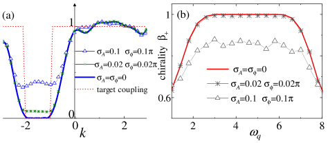
Figure 2: (a) The averaged $k$-space coupling coefficient $G_{k}$ for the sequence in Fig. 1 under different disorder strengths. (b) Chiral factor $\beta_{+}$ changes with $\omega_{q}$ in the presence of the disorder in (a).

Broadband chiral emission—

We proceed to study the broadband chiral emission by designing $g(x_{i})$ based on the proposed optimized procedure. Contrasting previous studies on chiral quantum optics targeting only on a single frequency Mitsch et al. (2014); Petersen et al. (2014), our proposal can route directionally photons in a broadband frequency regime with a large bandwidth of the chiral channel. The amplitudes $A(x_{i})$ and phases $\theta(x_{i})$ of the coupling sequence are depicted in Fig. 1. The total coupling points are $N=10$. The giant atom’s size $L=x_{N}-x_{1}<2\lambda_{0}$. It is much smaller than the width of the photonic wavepacket emitted from any single point at $x_{i}$. Therefore, the time-delay effect can be neglected sup . As depicted in Fig. 2(a), inside the asymmetric gap, the optimized $G_{k}$ is approximately zero, and matches the target coupling function.

The chiral factor $\beta_{\pm}$ can be derived by employing the Weisskopf-Wigner theory sup

$$\beta_{\pm}=\frac{|G_{\pm k_{r}}|^{2}}{|G_{k_{r}}|^{2}+|G_{-k_{r}}|^{2}},$$ (4)

where $k_{r}=\omega_{q}/c$, $G_{\pm k_{r}}$ are the coupling strengths at the resonant positions, and $+(-)$ corresponds to the right (left) propagating mode. The asymmetric coupling with $G_{k_{r}}\gg G_{-k_{r}}$ indicates a right chiral emission. Moreover, the asymmetric regime is very broad [see Fig. 2(b)], indicating a broadband chiral emission. When $\omega_{q}$ varies in a wide frequency regime, the chiral factor always approaches $\beta_{+}\simeq 1$. Such broadband chiral behavior has not yet reported in other quantum setups. For example, the chiral bandwidth of nanophotonic structures is equal to the Lorentzian transmission width of the emitter, which is much narrower than that in our proposal Coles et al. (2016).

For the experimental realization of our setup, the fabrication errors can perturb the optimized coupling sequence. To include this disorder effect, we add random perturbations to the coupling strength as $g(x_{i})\rightarrow[A(x_{i})+\delta A(x_{i})]e^{i[\theta(x_{i})+\delta\theta(x_{i})]}.$ The random offsets are sampled from Gaussian distributions with amplitude (phase) disorder width $\sigma_{\alpha}A(x_{i})$ ($\sigma_{\phi}$). We plot the disorder averaged $k$-space coupling for different $\{\sigma_{A},\sigma_{\phi}\}$, as shown in Fig. 2(a). The asymmetric band gap is lifted due to disorders. The evolution shows that the chiral factor is approximately one in a very wide frequency range for disorder strengths $\{\sigma_{A}=0.02,\sigma_{\phi}=0.02\pi\}$ [see Fig. 2(b)]. Even with stronger disorders, i.e., $\{\sigma_{A}=0.1,\sigma_{\phi}=0.1\pi\}$, the chirality remains above $0.85$, indicating that the broadband chiral emission realized in our proposal is robust to fabrication errors in the coupling sequence.

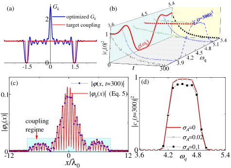
Figure 3: (a) The optimized and target coupling functions for realizing a band-gap environment. (b) Time evolution of $|c_{e}(t)|^{2}$ for different atomic frequency $\omega_{q}$. (c) The photonic part of the bound state by setting $\omega_{q}=4.5$ (in the band gap). (d) In the present of different disorder strengths, the trapped population $|c_{e}(t)|^{2}$ ($t=300$) changes with $\omega_{q}$.

Bound states.—

Given that the QED setup is constructed via conventional linear elements, the local phase $\theta(x_{i})\equiv 0$, and $G^{*}_{k}=G_{-k}$ is valid. In this case, $\forall g(x_{i})\geq 0$ should be added in the constraint conditions sup . $G_{k}$ is zero only in a narrow band with width $k_{d}$ around $\pm k_{0}$, otherwise it remains a constant [see Fig. 3(a)]. This scenario is very similar to an atom interacting with a waveguide environment with band gaps in periodic structures. By setting $k_{0}=1.5$ and $k_{d}=0.1$, we employ the same method for broadband chiral emission by searching the sets $\{x_{i},g(x_{i})\}$, and the optimized $G_{k}$ is depicted in Fig. 3(a). The optimal sequence is discussed in Ref. sup . In addition, the weight function inside the band gap is set to be much larger than the outside parts. A small number of coupling points $N=28$ is required with $g(x_{i})$ being of the same sign. Owing to suppression effects of the unbalanced weight function, the remnant coupling in the gap area is approximately zero, which can exactly mimic a band-gap environment.

We will show that our setup shares the same QED phenomena as conventional light-matter hybrid structures with photonic band gaps. We mainly focus on the fractional decay and bound state of the setup. In the single-excitation subspace, considering an initial excitation in the giant atom, the time-dependent state vector of the hybrid system is $|\psi(t)\rangle=\sum_{k}c_{k}(t)|g,1_{k}\rangle+c_{e}(t)|e,0\rangle$. The evolutions of the atomic population $|c_{e}(t)|^{2}$ are shown in Fig. 3(b) for different $\omega_{q}$. There, $|c_{e}(t)|^{2}$ shows fractional decay with most energy being trapped inside the atom when $\omega_{q}$ is in the band gap. The trapped population is approximately $|c_{e}(t\rightarrow\infty)|^{2}\simeq(1+\sum_{k}{\left|G_{k}/\Delta_{k}\right|^{2}})^{-2}$. Once $\omega_{q}$ is shifted far away from the gap area, $|c_{e}(t)|^{2}$ can exponentially decay to zero.

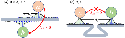
Figure 4: A QED setup where two giant atoms $a,b$ interact with the same waveguide. (b) When two atoms’ bound states overlap with each other, their dipole-dipole exchange rate is nonzero. (b) Relative to (a), two giant atoms decouple with each other when their coupling regimes are separated.

Moreover, there exists a static bound state with its wavefunction localized around the atom. As derived in Ref. sup , the real-space distribution for the photonic part of the bound state is

$$\psi_{b}(x)\propto\int_{\infty}^{\infty}dk\frac{G_{k}}{\Delta_{k}}e^{kx}=\sum_{i=1}^{N}\int_{-\infty}^{\infty}\frac{g(x_{i})}{\Delta_{k}}e^{k(x-x_{i})}dk.$$ (5)

In Fig. 3(c), we plot the field distribution by solving the system evolution to $t=500$, which is well described by the stable bound state obtained in Eq. (5). All the above phenomena are very similar to those observed in setups with band-gap environments Goban et al. (2014); Douglas et al. (2015, 2016); Hood et al. (2016); González-Tudela et al. (2015). The counterintuitive phenomenon is that there is no stable bound state if a small atom is coupled to the conventional waveguide. While, for giant atoms coupled to the waveguide, fields emitted from different coupling points interfere with each other [see Eq. (5)], which results in a time-independent $\phi_{b}(x)$. Note that, in our discussion, the propagating time inside the giant atom is negligible sup . Since the waveguide supports only modes with nonzero group velocity, the wavepacket outside the coupling regime cannot be reflected by any point and will propagate away. Therefore, $\phi_{b}(x)$ exactly lies within the coupling regime. This is different from its counterpart in structured environments. The structured environment supports modes with zero group velocity Douglas et al. (2015); González-Tudela et al. (2015); Bello et al. (2019), $\phi_{b}(x)$ can spread far away from the coupling point.

To include disorder effects, we sample the error $\delta\!g(x_{i})$ randomly from a Gaussian distribution centered around zero with width $\sigma_{A}g(x_{i})$. We plot the disorder averaged excitation being trapped inside the atom versus $\omega_{q}$ ($t=300$), as shown in Fig. 3(d). The averaged coupling inside the gap becomes non-zero due to the random noise  sup . Therefore, the protection from the band gap is destroyed, and $|c_{e}(t)|^{2}$ decays. The decoherence rate increases with growing $\sigma_{A}$, as shown in Fig. 3(d). However, for $\sigma_{A}<0.1$, the evolution is only slightly affected by disorders. Detailed discussions about disorder effects are presented in Ref. sup .

Dipole-dipole interactions.—

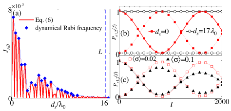
Figure 5: (a) The dipole-dipole interaction strength vs. the separation distance $d_{s}$ ($\omega_{q}=4.4$). (b) The Rabi oscillations for $d_{s}=0$ and $d_{s}=17\lambda_{0}>L$, respectively. (c) The dissipative Rabi oscillations under different disorder strengths.

We now include two giant atoms coupled to the same waveguide with the optimal coupling sequence, and explore the atom-atom interaction. By tracing out the photonic degree of freedom sup , the Hamiltonian of the effective dipole-dipole interaction is $H_{d-d}=J_{AB}(\sigma^{+}_{2}\sigma^{-}_{1}+\text{H.c.})$, with:

$$J_{AB}=\int_{\infty}^{\infty}\frac{|G^{\prime}_{k1}|^{2}e^{ikd_{s}}}{\Delta_{k}}dk,\quad G^{\prime}_{k1}=G_{k1}\sqrt{\frac{L_{w}}{2\pi}},$$ (6)

where $L_{w}\rightarrow\infty$ is the waveguide’s length adopted in the numerical simulations. A long waveguide is utilized to avoid photons being reflected by the boundary. In Eq. (6), we assume that the coupling sequence of atom $b$ is the same with $a$, translated a distance $d_{s}$ to $a$. Figure 5(a) depicts $J_{AB}$ versus $d_{s}$ [Eq. (6)], which matches well the numerical dynamical evolutions [obtained from the two atoms’ Rabi oscillating frequency $2J_{AB}$, see Fig. 5(b)]. When $\omega_{q}$ lies in the band gap, due to the protection of the band gap effects, both collective and individual decays are zero. and the dipole-dipole exchange is free of decoherence.

Equation (6) also indicates that the dipole-dipole interaction is proportional to the overlap area between the two bound states (see Fig. 4). Since each bound state’s distribution area coincide with the coupling regime, $J_{AB}$ is nonzero only when two atoms’ coupling regimes overlap with each other. The dipole-dipole interaction vanishes when $d_{s}$ is larger than the coupling distance $L$ ($L=17\lambda_{0}$), as depicted in Fig. 4(b). We also consider two coupling sequences both experiencing independent disorders, the average Rabi oscillations are shown in Fig. 5(c). For $\sigma_{A}\simeq 0.02$, the decay of the exchange process is not apparent, and the two atoms can coherently exchange excitations with a high fidelity.

Conclusion.—

In this work, we explore the possibilities to realize quantum optics in structured photonic environments with giant atoms. We show that most phenomena can be reproduced by designing the couplings between giant atoms and conventional environments without any nanostructure. We first introduce a generic method to find the optimized coupling sequences for arbitrary structured light-matter interaction. Given that a position-dependent phase is added to each coupling point, the giant atom can chirally emission photons in a very wide frequency regime, which has no analog in other quantum setups. We also show that the quantum effects in a band-gap environment (such as atomic fractional decay, static bound state and non-dissipative dipole-dipole interactions) can all be observed. Numerical results indicate that all the above QED phenomena can be observed even in the present of fabrication disorder in coupling sequences. Our proposed methods are very general and can also realize other types of structured environments, e.g., with multiple band gaps or a narrow spectrum bandwidth. Other quantum effects in those artificial environments, such as non-Markovian dynamics or multi-photon processes, can also be revisited Shi et al. (2016); Mahmoodian et al. (2018, 2020); Kusmierek et al. (2022), and new quantum effects might be observed.

Acknowledgments.— We thank Dr. A. F. Kockum for discussions and useful comments. The quantum dynamical simulations are based on open source code QuTiP Johansson et al. (2012, 2013). X.W. is supported by the National Natural Science Foundation of China (NSFC) (Grant No. 12174303 and No. 11804270). T.L. acknowledges the support from National Natural Science Foundation of China (Grant No. 12274142), the Startup Grant of South China University of Technology (Grant No. 20210012) and Introduced Innovative Team Project of Guangdong Pearl River Talents Program (Grant No. 2021ZT09Z109). F.N. is supported in part by: Nippon Telegraph and Telephone Corporation (NTT) Research, the Japan Science and Technology Agency (JST) [via the Quantum Leap Flagship Program (Q-LEAP), and the Moonshot R&D Grant Number JPMJMS2061], the Asian Office of Aerospace Research and Development (AOARD) (via Grant No. FA2386-20-1-4069), and the Foundational Questions Institute Fund (FQXi) via Grant No. FQXi-IAF19-06.

Supplementary Material for
Realizing Quantum Optics in Structured Environments with Giant Atoms

Xin Wang¹, Huai-Bing Zhu¹, Tao Liu² and Franco Nori^3,4,5

¹ Institute of Theoretical Physics, School of Physics, Xi’an Jiaotong University, Xi’an 710049, People’s Republic of China
² School of Physics and Optoelectronics, South China University of Technology, Guangzhou 510640, China
³RIKEN Center for Quantum Computing, Wakoshi, Saitama 351-0198, Japan
⁴Theoretical Quantum Physics Laboratory, RIKEN Cluster for Pioneering Research, Wako-shi, Saitama 351-0198, Japan
⁵Physics Department, The University of Michigan, Ann Arbor, Michigan 48109-1040, USA

This supplementary material includes the following: In Sec. I, we first discuss the limitations of the inverse Fourier transformation (iFT) method for obtaining the real-space coupling of a target $k$-space interaction. Then we introduce the numerical optimization method under physical constraints. In Sec. II, we focus on how to realize the band-gap effect with the optimized coupling sequence. Unconventional phenomena (such as trapped bound state, fractional decay, and dipole-dipole interaction) are investigated. By employing numerical simulation methods, we discuss how disorder in the coupling sequences affect our proposal. In Sec. III, by adding synthetic phases at coupling points, we obtained the optimized coupling sequence for broadband chiral emission. The disorder effects of coupling amplitudes and phases are addressed.

S1 Optimized real-space coupling for band-gap environments

We now present a generic optimization algorithm to find the desired coupling sequence. In the main text, we start our discussions with the example of realizing broadband chiral emission, which require optimizing the local phase sequence $\theta(x_{i})$. In experiments, the additional phase $\theta(x_{i})$ at $x_{i}$ can be realized by time-dependent modulating the nonlinear coupling elements. However, in this supplementary material, we will show that there is no local phase and all coupling strengths $g(x_{i})$ are of the same sign, given that the QED setup is mediated by conventional linear elements. In this case, the corresponding algorithm is more complex and needs much more time due to the lack of phase freedom. Therefore, we take the band-gap environment as an example, to introduce our proposed optimization method.

S1.1 Analytical method and its problems

We assume giant atoms interacting with a 1D waveguide, which has a linearized dispersion within the photonic bandwidth to which the giant atom significantly couples, i.e., $\omega_{k}=c|k|$ with $c$ being the phase (group) velocity. As discussed in the main text, the following $k$-space coupling function equivalently describes an atom interacting with a band-gap environment

$$G^{I}_{k}=\begin{cases}0\qquad\left\{k_{0}-\frac{k_{d}}{2}<|k|<k_{0}+\frac{k_{d}}{2}\right\},\\ G_{0}\qquad\left\{k_{0}+\frac{k_{d}}{2}<|k|<k_{\text{max}}\right\}\cup\left\{-k_{0}+\frac{k_{d}}{2}<k<k_{0}-\frac{k_{d}}{2}\right\}.\\ \end{cases}$$ (S1)

That is, the gap’s width is $k_{d}$ and is centred at $\pm k_{0}$. The coupling constant is denoted by $G_{0}$. For convenience the ultraviolet cut-off frequency is set at $ck_{\text{max}}$, which should be large enough to approximate the regime $\left\{k_{0}+\frac{k_{d}}{2}<|k|<k_{\text{max}}\right\}$ as an infinite bandwidth environment.

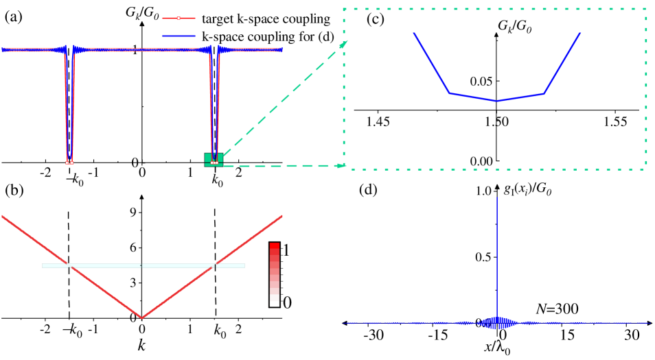
Figure S1: (a) The $k$-space coupling for the real-space sequence by discretizing $g_{I}\left(x\right)$ in Eq. (S2) [see plot in (d)]. The target coupling function has two symmetric dips centred at $k_{0}=\pm 1.5$ with width $k_{d}=0.1$. (b) The waveguide is assumed to be of linear dispersion with a phase velocity $c=3$. The coupling strength $G_{k}$ in (a) is mapped with color, where two symmetric dips around $k_{0}$ are equivalent to band gaps in a structured environment. (c) The enlarged plot around $k_{0}$ of plot (a). Inside the band gap there is still remnant non-zero coupling ($\sim 0.02G_{0}$) even with a large sampling number $N=300$. (d) Real-space coupling sequence $g(x_{i})$ (with $N=300$). The sampling interval and total length are set as $X_{T}=1$ and $L=35\lambda_{0}$, respectively.

The inverse Fourier transform (iFT) of $G^{I}_{k}$ is derived as

$$g_{I}\left(x\right)=\frac{\sin k_{\max}x}{\pi x}-2\frac{\sin k_{d}x/2}{\pi x}\cos k_{0}x,$$ (S2)

which is a continuous function in real space. In experiments, giant atoms usually couple at multiple discretized positions on a waveguide. Therefore, we assume that the coupling function $g_{I}\left(x\right)$ is sampled by the following function

$$S(x)=W\left(x\right)P(x),\quad W\left(x\right)=\left\{\begin{array}[]{c}1\quad|x|\leq L,\\ 0\quad|x|>L,\\ \end{array}\right.\quad P(x)=\sum_{n=-\infty}^{n=+\infty}\delta\left(x-nX_{T}\right),$$ (S5)

where $W\left(x\right)$ is a window function with a width $2L$, and $P(x)$ is the sample sequence composed by $\delta$-function series which are equally spaced with distance $X_{T}$. To avoid retardation effects, the total coupling length $2L$ (i.e., the giant atom’s size) should be much smaller than the size of the decaying photonic wavepacket Guo et al. (2020). All those physical restraints will be addressed in later discussions.

According to the convolution theorem, the Fourier transformation of $S(x)$ is written as

$$S(k)=W\left(k\right)*\Delta(k),\quad W\left(k\right)=2\frac{\sin(kL)}{k},\quad P(k)=\frac{2\pi}{X_{T}}\sum_{n=-\infty}^{n=\infty}\delta(k-\frac{2\pi n}{X_{T}}),$$ (S6)

where $*$ represents the convolution of two functions. Equation (S6) indicates that the width of the $\delta$-functions $\delta(k-\frac{2\pi n}{X_{T}})$ in $k$-space are broadened as $\sim 2\pi/L$. To resolve the narrow band gap, the following relation should be satisfied

$$2\pi/L\ll k_{d}\,\,\longrightarrow L\,\,\gg\frac{2\pi}{k_{d}}.$$ (S7)

Additionally, to avoid spectrum aliasing effect, the sample distance is bounded by the Nyquist–Shannon sampling theorem

$$\frac{2\pi}{X_{T}}\gg 2k_{\text{max}}\,\,\longrightarrow\,\,X_{T}\ll\frac{\pi}{k_{\text{max}}}.$$ (S8)

Consequently, the coupling number of the giant atom is bounded by

$$N=\frac{2L}{X_{T}}\gg\frac{4k_{\text{max}}}{k_{d}}.$$ (S9)

We now consider the target $k$-space coupling function with $k_{\text{max}}=3$, $k_{0}=1.5$ and $k_{d}=0.1$ [see Fig. S1(a)]. According to Eq. (S9), the minimum coupling number is calculated as $N=120$. In Fig. S1(d), we plot the sampled real-space coupling sequence by setting $N=300$. The corresponding $k$-space coupling function is shown in Fig. S1(a), and the amplitude is mapped with color in Fig. S1(b). Note that $\lambda_{0}=2\pi/k_{0}$ is the wavelength of the central mode in the gap, and is employed as the unit length in this work. To mimic the band gap, the most important feature of $G_{k}$ is the vanishing of the coupling strength around $k_{0}$. The enlarged plot of this regime is depicted in Fig. S1(c), which shows that the remnant coupling is still about $0.02G_{0}$. In principle one can keep increasing both $N$ and $L$ to suppress the non-zero coupling. However, much more coupling points are need, which is very challenging in experiments. Moreover, given that $L$ is comparable to the wavepacket decaying from a single point, the propagating time cannot be neglected.

We also note that the coupling strengths $g(x_{i})$ which are sampled from Eq. (S2), alter their signs [see Fig. S1(d)]. That is, $g(x_{i})$ needs an additional $\pi$-phase difference, which leads to another problem when implementing the coupling sequence in experiments. We now consider the circuit-QED as an example, where giant atoms are mostly discussed. As depicted in Fig. S2, a transmon (working as a giant atom) is capacitively coupled to a 1D waveguide at multiple points. As discussed in Ref. Koch et al. (2007); You et al. ; Gu et al. (2017), the interaction Hamiltonian of the whole setup is written as

$$H_{\text{int}}=\sum_{k}\hbar\Delta_{k}a^{\dagger}_{k}a_{k}+\sum_{k}\hbar\left(G_{k}a_{k}^{\dagger}\sigma_{-}+\text{H.c.}\right),$$ (S10)

$$G_{k}=\sum_{x_{i}}g(x_{i})e^{-ikx_{i}},\quad g(x_{i})=\frac{e}{\hbar}\frac{C_{g}(x_{i})}{C_{\Sigma}}\sqrt{\frac{\hbar\omega_{k}}{C_{t}}}\simeq\frac{e}{\hbar}\frac{C_{g}(x_{i})}{C_{\Sigma}}\sqrt{\frac{\hbar\omega_{q}}{C_{t}}},$$ (S11)

where $C_{J}$ is the Josephson capacitance of the transmon, $C_{g}(x_{i})$ is the coupling capacitance at point $x_{i}$, $C_{\Sigma}=C_{J}+\sum_{i}C_{g}(x_{i})$, and $C_{t}$ is the total capacitance of the waveguide. In Eq. (S11) we replace $\omega_{k}\rightarrow\omega_{q}$ for the zero-point fluctuations of the voltage operators because only modes around $\omega_{q}$ contribute significantly to the dynamics. Under this condition, the local coupling strength $g(x_{i})$ is proportional to the coupling capacitance $C_{g}(x_{i})$, and the coupling sequence in Fig. S1(d) can be directly encoded into $C_{g}(x_{i})$ [see Fig. S2]. We notice that the coupling signs of $g(x_{i})$ are fixed because $\{C_{g}(x_{i}),C_{\Sigma}\}\geq 0$. That is, there are no additional $\pi$-phase differences between different coupling points, and the discretized coupling obtained via the iFT method cannot be implemented with a linear coupling capacitance (or inductance). The additional local phase $\theta(x_{i})$ can be encoded at $x_{i}$ via the time-dependent modulating of the nonlinear QED elements, which however will add more overheads in the experiments Chen et al. (2014); Wulschner et al. (2016); McKay et al. (2016); Roushan et al. (2017); Kounalakis et al. (2018); Yan et al. (2018); Joshi et al. (2022),

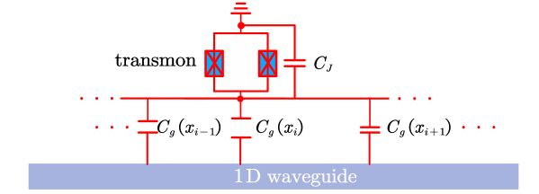
Figure S2: Sketch of a feasible setup to realize our proposal: a transmon couples to a 1D coplanar waveguide at multiple coupling points via local capacitances $C_{g}(x_{i})$. The real-space discretized coupling function is encoded into the capacitance sequence $C_{g}(x_{i})$.

In conclusion, to realize a structured environment with a giant atom, the analytical iFT method has the following problems:

1) Too many coupling points might be needed, which is challenging for the experimental realization.

2) The remnant non-zero coupling in the band gaps is still high.

3) The coupling strengths alter their signs, which is unfeasible with the linear coupling elements used in the experiments.

S1.2 Optimization method

To solve the above problems, we consider the coupling function inside and outside the gap separately. The coupling strength should be exactly zero inside the gap area, which is the most important feature for a band-gap environment. Outside the band gap area, even if the interaction varies with $k$ slightly (of the same order), the dynamics, such as trapped bound state and non-exponential decay led by band gaps, can still be observed. For the modes far away from the gap, strong coupling strengths do not affect the system’s evolution due to large detuning relations. Therefore, the constraint requiring the $k$-space coupling strength outside the band gap to be identical, is too strong. All these indicate that the desired $k$-space coupling can be obtained even when the real-space coupling strengths are of the same sign. Moreover, relaxing the conditions by allowing $G_{k}$ to vary with $k$ can also reduce the required number of coupling points.

Now we convert realizing the target $k$-space coupling function as an optimization problem, which can be solved numerically. The constraint conditions for this problems are summarized as follows:

$$\begin{cases}1.\qquad\forall g(x_{i})\geq 0,\\ 2.\qquad\eta\lambda_{0}<\min\left\{x_{i+1}-x_{i}\right\},\\ 3.\qquad-\frac{L}{2}<x_{1}<x_{N}<\frac{L}{2},\quad L\ll\bar{L}_{0},\quad\bar{L}_{0}=\frac{1}{N}\sum_{i}^{N}L_{i}.\\ 4.\qquad N\leq N_{\text{max}},\\ \end{cases}$$ (S12)

Condition 1 restricts that all real-space coupling strengths are of the same sign, which avoids the coupling sign problem in QED setups with linear couplers.

Condition 2 sets the lower bound of the distance between two neighbor points. The reason for this restriction is that the coupling is mediated via physical elements with finite sizes (for example, capacitances or inductances in circuit-QED). Due to fabrication limitations and to avoid crosstalk, two neighbouring points cannot be too close to each other.

In condition 3, $L_{i}$ is the size of a decaying photonic wavepacket from a small atom which just couples to the waveguide at a single point $g(x_{i})$, and $\bar{L}_{0}$ is the average size of all the decaying wavepackets. This restriction guarantees that the re-absorption and re-emission of photons due to time retardation can be neglected.

Condition 4 sets the maximum coupling number, which is much smaller than that bounded by Eq. (S9).

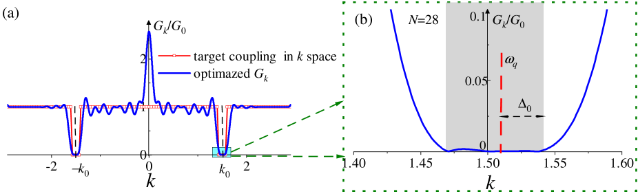
Figure S3: (a) The $k$-space coupling function $G_{k}$ for the real-space sequence in Table 1. (b) Enlarged plot around $k_{0}$. The detuning between $\omega_{q}$ and the band edge is denoted as $\Delta_{0}$.

Considering a real-space sequence $g^{\prime}(x_{i})$ satisfying condition (1-4), its $k$-space coupling function is denoted as $G^{\prime}(k)$, which is obtained from Eq. (S11). To find the optimized real-space sequence, we define an objective function

$$C_{m}=\int_{-k_{\text{max}}}^{k_{\text{max}}}dk||G^{\prime}(k)|-|G^{I}(k)||w(k),$$ (S13)

which can quantify the difference between the obtained $G^{\prime}(k)$ and the target coupling function. In Eq. (S13) we introduce a weight function $w(k)$ to control the similarities for modes in different regimes. For simplicity, we assume $w(k)$ to be

$$w(k)=\begin{cases}w_{1}\qquad\left\{k_{0}-\frac{k_{d}}{2}<|k|<k_{0}+\frac{k_{d}}{2}\right\},\\ w_{0}\qquad\left\{k_{0}+\frac{k_{d}}{2}<|k|<k_{\text{max}}\right\}\cup\left\{-k_{0}+\frac{k_{d}}{2}<k<k_{0}-\frac{k_{d}}{2}\right\}.\\ \end{cases}$$ (S14)

Since the likehood between $G^{\prime}(k)$ and $G^{I}(k)$ in the band gap regime is much more important, we set $w_{1}\gg w_{0}$ in Eq. (S13). The optimization process minimizes $C_{m}$ by searching the possible functions $g(x_{i})$ satisfying the constraint condition in Eq. (S12).

position ($x_{i}/\lambda_{0}$)	$-$8.196	$-$7.901	$-$6.992	$-$6.682	$-$4.721	$-$4.396	$-$3.726	$-$3.419	$-$2.732	$-$2.441
coupling strength	0.0184	0.0291	0.0268	0.0146	0.0306	0.0502	0.0302	0.086	0.0317	0.1206
position ($x_{i}/\lambda_{0}$)	$-$1.71	$-$1.46	$-$0.507	$-$0.006	0.244	0.544	1.488	2.459	3.439	4.448
coupling strength	0.0906	0.0748	0.0223	0.1413	0.1553	0.9543	0.0458	0.1441	0.1305	0.1152
position ($x_{i}/\lambda_{0}$)	4.861	5.44	5.88	6.383	6.846	7.166	7.857	8.168
coupling strength	0.0298	0.0393	0.0402	0.0219	0.0472	0.0184	0.0366	0.0265

Table 1: The real-space coupling sequence obtained via the optimized method proposed in this work. The corresponding $k$-space coupling is shown in Fig. S3(a).

In this work we set $L\simeq 17\lambda_{0}$, $\eta=0.1\lambda_{0}$, $N_{\text{max}}=30$, and $w_{1}=60w_{0}$, and the obtained coupling sequence $g(x_{i})$ (of the same sign) is listed in Table 1. The corresponding $k$-space coupling is shown in Fig. S3(a), and the enlarged plot around the band gap is in Fig. S3(b). We find that the number of points is reduced as $N=28$, and the remnant non-zero coupling in gap area is decreased below $10^{-4}G_{0}$, which is much weaker than those in Fig. S1(c). Specially, $G_{k}$ varies slightly with $k$ for the modes outside the band gap, and the dc part (around $k\simeq 0$) will strongly couple to the giant atom because the $g(x_{i})$’s signs are the same [see Fig. S3(a)]. To demonstrate the band-gap effect, the atomic frequency is usually set around $ck_{0}$, and therefore, the interaction with those low-frequency components is negligible due to large detuning effects, which can be verified from the numerical discussion in next section.

S2 QED phenomena in band-gap environments

S2.1 Fractional decay and bound states

We show that most QED phenomena in band-gap environments can be reproduced with our proposal. In numerical simulations, the mode number in the regime $-k_{\text{max}}<k<k_{\text{max}}$ is discretized with an interval $\delta\!k=10^{-3}$, which is equal to considering a waveguide with length $L_{w}=2\pi/\delta k\simeq 6.28\times 10^{3}$. Such a long waveguide guarantees the propagating wavepacket never touches the boundary. We first estimate the size of the decaying wavepacket for a single coupling point. According to the Weisskopf-Wigner theory, given that a small atom coupling at point $x_{i}$, the decay rate and the corresponding wavepacket size are respectively derived as

$$\Gamma_{i}=\frac{2\pi|g^{\prime}_{x_{i}}|^{2}}{c},\quad g^{\prime}_{x_{i}}=g(x_{i})\sqrt{\frac{L_{w}}{2\pi}},\quad L_{i}\simeq 2c\Gamma^{-1}_{i}.$$ (S15)

The coupling constant is set as $G_{0}=0.002$ in our discussion. By employing the coupling sequence in Table 1, the maximum and average sizes of the wavepacket are respectively calculated as $\max\{L_{i}\}\simeq 2\times 10^{2}\lambda_{0}$ and $\bar{L}_{0}\simeq 8\times 10^{4}\lambda_{0}$, which are both much larger than the giant atom’s size $L$. Therefore, we can neglect the time retardation effects.

Assuming a single excitation initially trapped inside the giant atom, the system’s state at time $t$ is expanded as $|\psi(t)\rangle=\sum_{k}c_{k}(t)|g,1_{k}\rangle+c_{e}(t)|e,0\rangle$. The dynamical evolution is numerically solved in this single-excitation subspace by discretizing the waveguide’s modes in $k$ space. A similar method can be found in Ref. Wang and Li (2022). We start from the evolution governed by the interaction Hamiltonian in Eq. (S10), which is derived as

$$\dot{c}_{e}\left(t\right)=-i\sum_{k}{G_{k}}c_{k}\left(t\right),$$ (S16)

$$\dot{c}_{k}\left(t\right)=-i\Delta_{k}c_{k}\left(t\right)-iG_{k}^{*}c_{e}\left(t\right).$$ (S17)

The above equations can be expressed in Laplace space as

$$s\tilde{c}_{e}\left(s\right)-c_{e}\left(t_{0}\right)=-i\sum_{k}{G_{k}}\tilde{c}_{k}\left(s\right),$$ (S18)

$$s\tilde{c}_{k}\left(s\right)-c_{k}\left(t_{0}\right)=-i\Delta_{k}\tilde{c}_{k}\left(s\right)-iG_{k}^{*}\tilde{c}_{e}\left(s\right),$$ (S19)

and the initial conditions are $c_{k}\left(t=0\right)=0$ and $c_{e}\left(t=0\right)=1.$ The time-dependent evolution is derived by the inverse Laplace transformation Ramos et al. (2016)

$$c_{e}\left(t\right)=\frac{1}{2\pi i}\lim_{E\rightarrow\infty}\int_{\epsilon-iE}^{\epsilon+iE}\tilde{c}_{e}\left(s\right)e^{st}ds,\quad\epsilon>0.$$ (S20)

Finally, we obtain

$$\tilde{c}_{e}\left(s\right)=\frac{1}{s-\Sigma_{e}(s)},\quad\Sigma_{e}(s)=\sum_{k}{\frac{-|G_{k}|^{2}}{s+i\Delta_{k}}}.$$ (S21)

where $\Sigma_{e}(s)$ is the self-energy of the giant atom. Given that the atomic frequency is in the gap area, part of the energy will be trapped inside the giant atom since there is no resonant pathway to radiate the excitation away. This point can also be verified from the roots of the transcendental equation $s-\Sigma_{e}(s)=0$, which correspond to the intersection points of $f(s)=s$ and $f(s)=\Sigma_{e}(s)$ [see Fig. S4(a)]. We find that there is only one pure imaginary solution $s_{0}$ (blue dots), which increases with $G_{0}$. Since $s_{0}$ is the imaginary pole for $\tilde{c}_{e}\left(s\right)$, it corresponds to a static bound state which does not decay with time Cohen-Tannoudji et al. (1998). In this scenario, part of the atomic energy will be trapped without decaying, and the steady amplitude of $c_{e}(t)$ can be obtained via the residue theorem

$$c_{e}(t\rightarrow\infty)=\text{Res}(s_{0})=\frac{1}{1-\partial_{s}\Sigma_{e}(s)}\Big{|}_{s=s_{0}}=\frac{1}{1-\sum_{k}{\frac{|G_{k}|^{2}}{(s_{0}+i\Delta_{k})^{2}}}}.$$ (S22)

In Fig. S4(b), we plot $|c_{e}(t\rightarrow\infty)|^{2}$ versus the coupling strength $G_{0}$, which matches well with $|\text{Res}(s_{0})|^{2}$. Given that the coupling strength is weak, most of the energy was trapped inside the atom, and the steady-state population is $|c_{e}(t\rightarrow\infty)|^{2}\simeq 1$. When increasing $G_{0}$, the trapped atomic excitation will decrease, and more energy will distribute on the waveguide.

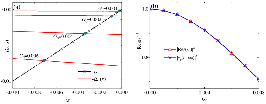
Figure S4: (a) The root of transcendental equation $s-\Sigma_{e}(s)=0$ can be numerically solved, which correspond to the intersection point (blue dots) for different values of $G_{0}$. (b) The excitation population trapped inside the atom $|\text{Res}(s_{0})|^{2}$ changes with $G_{0}$ [calculated via the residue theorem in Eq. (S22)], and matches well the dynamical evolution $|c_{e}(t\rightarrow\infty)|^{2}$. The atomic frequency is fixed at $\omega_{q}=4.5$.

We now show that the partial photonic field is trapped inside the coupling area without propagating away, which is akin to the bound state in QED setups with band-gap media. The bound state, which is the eigenstate of the system Hamiltonian, can be obtained by solving the following Schrödinger equation $H_{\text{int}}|\psi_{b}\rangle=E_{b}|\psi_{b}\rangle$, where $|\psi_{b}\rangle=\cos(\theta)|e,0\rangle+\sin\theta\sum_{k}c_{k}\mbox{$|g,1_{k}\rangle$}$, with $\theta$ being the mixing angle. The solution is obtain from the following equations:

$$c_{k} = \frac{G_{k}}{\tan\theta(E_{b}-\Delta_{k})},$$ (S23)

$$E_{b} = \sum_{k}\frac{|G_{k}|^{2}}{E_{b}-\Delta_{k}},$$ (S24)

$$\tan\theta = \sum_{k}\frac{|G_{k}|^{2}}{(E_{b}-\Delta_{k})^{2}}.$$ (S25)

Note that Eq. (S24) is the same with Eq. (S21) (by replacing $E_{b}$ with $is_{0}$). In our discussion, the interaction between the giant atom and the waveguide is weak. Therefore, the eigenenergy $E_{b}$ is around zero [i.e., $s_{0}\simeq 0$, see Fig. S4(a)]. Under this condition, most of the energy will be trapped inside the atom, and the mixed angle $\theta\simeq 0$ . Employing the approximations $\sin\theta\simeq\tan\theta$ and $E_{b}\simeq 0$, the photonic field is derived as

$$\psi_{b}(x)=\frac{\sin\theta}{\sqrt{L_{w}}}\sum_{k}c_{k}e^{kx}\simeq-\frac{\sqrt{L_{w}}}{2\pi}\int_{-\infty}^{\infty}\frac{G_{k}}{\Delta_{k}}e^{kx}dk.$$ (S26)

By substituting the real-space coupling in Eq. (S11) into $\psi(x)$, we rewrite $\psi_{b}(x)$ as

$$\psi_{b}(x)=-\frac{\sqrt{L}}{2\pi}\sum_{x_{i}}\phi_{bi}(x),\quad\phi_{bi}(x)=\int_{-\infty}^{\infty}\frac{g(x_{i})}{\omega_{k}-\omega_{q}}e^{k(x-x_{i})}dk.$$ (S27)

In Eq. (S27), $\phi_{bi}(x)$ is induced by a small atom which couples to the 1D waveguide at the single point $x_{i}$. In the weak-coupling regime, the small atom will exponentially decay all its energy into the waveguide given that $t\rightarrow\infty$. Therefore, there is no stable bound state for a small atom, which can also be explained by the behavior of $\psi_{bi}(x)$ in Eq. (S27), where

$$\lim\limits_{\omega_{k}\rightarrow\omega_{q}}\frac{g(x_{i})\,e^{-ikx_{i}}}{\omega_{k}-\omega_{q}}=\infty$$ (S28)

is divergent. That is, the expression for $\phi_{bi}(x)$ is non-integrable.

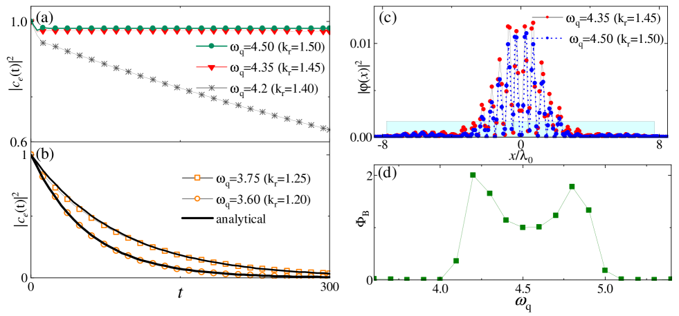
Figure S5: (a, b) Dynamical evolution of $|c_{e}(t)|^{2}$ for different atomic frequency. When $\omega_{q}$ is in the band gap, the atom only decays part of its energy into the waveguide. (c) The photonic field of the bound state for different atomic frequencies. The cyan box corresponds to the coupling regime. (d) The bound state’s photonic energy $\Phi_{b}$ changes with $\omega_{q}$, showing two peaks around the band edges.

The counterintuitive result is that a stable bound state appears when all the coupling points act simultaneously. The interference between different points prevents the giant atom from decaying, and results in a static bound state even when its frequency lies inside the continuum spectrum. In Fig. S5(a, b), by employing the coupling sequences in Table 1, we numerically plot $|c_{e}(t)|^{2}$ for different atomic frequencies. One finds that when $\omega_{q}$ is inside the band gap, the atom only decays part of its energy into the waveguide. In the steady state, most energy will be trapped inside the atom, and the bound state photonic field is plotted in Fig. S5(c). Around the band edge, where $G_{k}$ rises from 0 quickly, the atomic evolution is highly non-Markovian. Since the spectrum of a linear-dispersion waveguide has no point of zero group velocity, the wavepacket outside the coupling regime will propagate outside without traveling back. Therefore, $\psi_{b}(x)$ is exactly localized inside the coupling regime.

As depicted in Fig. S5(c), $\psi_{b}(x)$ also depends on the atomic frequency. Figure S5(d) depicts the photon energy trapped inside the bound state (defined as $\Phi_{B}=\int_{x_{1}}^{x_{N}}dx|\psi_{b}(x)|^{2}$) versus $\omega_{q}$. Due to the reduction of detuning, $\Phi_{B}$ reaches its highest value around the band edge (around $\omega_{q}\simeq 4.3$). Outside the band gap $\Phi_{B}$ decreases to zero quickly. When $\omega_{q}$ is far away from the band gap, the atom will exponentially dissipate its energy, which is well described by the Weisskopf-Wigner theory. Similar to Eq. (S15), the decay rate is

$$\Gamma=\frac{2\pi|G^{\prime}_{k_{r}}|^{2}}{c},\quad G^{\prime}_{k_{r}}=G_{k_{r}}\sqrt{\frac{L_{w}}{2\pi}},$$ (S29)

where $k_{r}=\omega_{q}/c$ is the resonant position, and $G^{\prime}_{k_{r}}$ is the normalized coupling strength. In Fig. S5(b) we numerically plot the evolution of $|c_{e}(t)|^{2}$, which fits well with the exponential decay derived from Eq. (S29).

S2.2 Simulating disorder effects

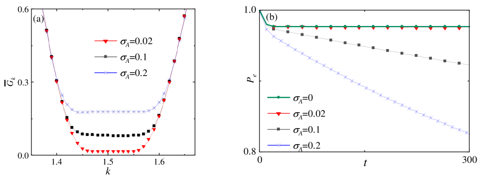
Figure S6: (a) The average $k$-space coupling $\bar{G}_{k}$ in the band-gap regime. (b) The disorder-averaged population $|\bar{p}_{e}(t)|$ changes with time under different disorder strengths. In each realization the random offsets are added into the optimal coupling sequence in Table 1. Here we set $\omega_{q}=4.5$, and the other parameters are the same with those in Fig. S5(a).

In experiments, fabrication errors can perturb the optimized coupling sequence. To simulate this, we add random offsets to the coupling sequence, i.e., $g(x_{i})\rightarrow g(x_{i})+\delta g(x_{i})$. Here $\delta g(x_{i})$ is sampled from a Gaussian distribution centered around zero and with a width $\sigma_{A}\,g(x_{i})$. Consequently, the average $k$-space coupling function is defined as

$$\bar{G}_{k}=\frac{1}{N_{\text{dis}}}\sum_{n=1}^{N_{\text{dis}}}\sum_{x_{i}}{[g(x_{i})+\delta g(x_{i})]e^{-ikx_{i}}},$$ (S30)

where $N_{\text{dis}}$ is the number of disorder realizations in numerical simulations. In our discussion, we set $N_{\text{dis}}=200$, which is large enough for the errors considered in this work. In Fig. S6(a), we plot $\bar{G}_{k}$ for different disorder strengths, and find that the band gap is lifted higher than zero.

To investigate the disorder effects on the quantum dynamics, we numerically simulate the evolution by taking the average of all the realizations. Defining the disorder averaged population as

$$\bar{p}_{e}(t)=\frac{1}{N_{\text{dis}}}\sum_{n=1}^{N_{\text{dis}}}\left|c_{e}(t)\right|^{2},$$ (S31)

we plot $\bar{p}_{e}(t)$ versus time by considering different disorder strengths in Fig. S6(b). The trapped excitation inside the atom becomes unstable and will slowly leak into the waveguide. The decoherence rate led by disorder increases with disorder strengths. It can be inferred that when $\sigma_{A}>0.2$, the protection effects of the band gap will be swamped by the disorder noise.

S2.3 Dipole-dipole interactions

Considering multiple giant atoms coupled to a common waveguide with the optimized sequences in Fig. 1, these atoms will interact with each other given that their bound states overlap with each other. We derive their dipole-dipole interaction strength by taking two giant atoms as an example. The Hamiltonian describing two giant atoms interacting with a common waveguide is expressed as

$$H_{\text{int2}}=\sum_{k}\hbar\Delta_{k}a^{\dagger}_{k}a_{k}+\sum_{i=1,2}\sum_{k}\hbar\left(G_{ki}a_{k}^{\dagger}\sigma^{-}_{i}+\text{H.c.}\right),$$ (S32)

where we assume two atoms’ transition frequencies to be identical, and $G_{ki}=\sum_{j}g_{i}(x_{j})G_{0}e^{-ikx_{ij}}$ is the coupling strength between giant atom $i$ and the waveguide. For simplicity, the optimized coupling sequences of two atoms are assumed to be the same, i.e., $g_{2}(x_{i})=g_{1}(x_{i}+d_{s})$ with $d_{s}$ being their separation distance. Given that their frequencies are in the band gap [see Fig. S3(b)], two atoms will exchange photons without decaying.

In principle, the exchange rate between two atoms can be tediously obtained by the standard resolvent-operator techniques Cohen-Tannoudji et al. (1998). This method is valid even when the atom-waveguide coupling enters into the strong coupling regime. Here we focus on the weak coupling regime, and the probability of photonic excitations in the waveguide is extremely low. In this case, the Rabi oscillating rate between two atoms corresponds to their interaction strength mediated by the waveguide’s modes, which can be simply derived via the effective Hamiltonian method James and Jerke (2007). Only the modes outside the band gap interact with two atoms, and the dipole-dipole interacting Hamiltonian mediated by one mode $k$ is derived as

$$H_{d-d,k}=\frac{G_{k1}G^{*}_{k2}}{\Delta_{k}}(\sigma^{-}_{1}a_{k}^{\dagger}\sigma^{+}_{2}a_{k}-\sigma^{+}_{2}a_{k}\sigma^{-}_{1}a_{k}^{\dagger})+\text{H.c.}$$ (S33)

The waveguide is just virtually excited and the photonic population is approximately zero. Therefore, by adopting the following approximations $\langle a_{k}^{\dagger}a_{k}\rangle\simeq 0$ and $\langle a_{k}a_{k}^{\dagger}\rangle\simeq 1,$ we can trace off the photonic freedoms in Eq. (S33), and simplify Eq. (S33) as

$$H_{d-d,k}\simeq-\frac{G_{k1}G^{*}_{k2}}{\Delta_{k}}\sigma^{+}_{2}\sigma^{-}_{1}+\text{H.c.}$$ (S34)

Note that the interaction Hamiltonian $H_{d-d,k}$ in Eq. (S34) is only mediated by one mode $k$. By taking all the modes’ contributions into account, we derive the total dipole-dipole interaction as

$$H_{d-d}=J_{AB}(\sigma^{+}_{2}\sigma^{-}_{1}+\text{H.c.}),\quad J_{AB}=-\sum_{k}\frac{G_{k1}G^{*}_{k2}}{\Delta_{k}}=\frac{L_{w}}{2\pi}\int_{-\infty}^{\infty}\frac{|G_{k1}|^{2}e^{ikd_{s}}}{\Delta_{k}}dk,$$ (S35)

where we adopt the translation relation between two coupling sequences, i.e., $G_{k2}=G_{k1}e^{-ikd_{s}}$. From Eq. (S35) and Eq. (S26), one can find that the coherent exchange channel is proportional to the overlap area between two bound states. In the main text, Fig. 4(a) depicts how $J_{AB}$ changes with $d_{s}$.

S3 Broad-band chiral emission

position ($x_{i}/\lambda_{0}$)	$-$0.909	-0.757	$-$0.383	$-$0.508	$-$0.0975	$-$0.222	0.393	0.120	0.641	0.909
amplitude $A(x_{i})$	0.088	0.130	0.628	0.429	0.392	0.591	0.365	0.198	0.615	0.243
phase $\theta(x_{i})$	0.388$\pi$	$-$0.500$\pi$	$-$0.446$\pi$	0.500$\pi$	$-$0.500$\pi$	0.500$\pi$	$-$0.500$\pi$	0.179$\pi$	0.0048$\pi$	0.460$\pi$

Table 2: The amplitudes and phases of the coupling sequence in Fig. 5 of the main text, which is obtained via the proposed optimization method.

In above discussions, we assume that the coupling strength $g(x_{i})$ are real and of the same sign, which can be realized in experiments with linear QED elements. In this case, the $k$-space interaction satisfies $G_{k}=G^{*}_{-k}$, indicating that the spontaneous emission rates into the right ($k>0$) and left directions ($k<0$) are identical. Therefore, the photonic field along the waveguide has no chiral preference. Given that additional local phases are generated via synthetic methods, i.e., $g(x_{i})=A(x_{i})e^{i\theta(x_{i})}$, the relation $|G_{k}|=|G_{-k}|$ is not valid again. In circuit-QED this additional phase can be realized via nonlinear Josephson junctions. As demonstrated in Ref. Chen et al. (2014); Wulschner et al. (2016); Roushan et al. (2017), by applying a time-oscillating flux signal with phase $\theta(x_{i})$ through the coupling loop at point $x_{i}$, the local phase $\theta(x_{i})$ were successfully encoded into the coupling point.

As discussed in the main text, we aim to realize chiral emission in a wide frequency range. Similarly to realizing band-gap effects, we first define a target function:

$$G^{I}_{k}=\begin{cases}0\qquad\left\{-k_{0}-\frac{k_{d}}{2}<k<-k_{0}+\frac{k_{d}}{2}\right\},\\ G_{0}\qquad\left\{-k_{\text{max}}<k<-k_{0}-\frac{k_{d}}{2}\right\}\cup\left\{-k_{0}+\frac{k_{d}}{2}<k<k_{\text{max}}\right\},\\ \end{cases}$$ (S36)

where the chiral bandwidth is $k_{d}$ [see Fig. S7(a)]. We define a weight function during the optimizing process

$$w(k)=\begin{cases}w_{1}\qquad\left\{-k_{0}-\frac{k_{d}}{2}<k<-k_{0}+\frac{k_{d}}{2}\right\},\\ w_{0}\qquad\left\{-k_{\text{max}}<k<-k_{0}-\frac{k_{d}}{2}\right\}\cup\left\{-k_{0}+\frac{k_{d}}{2}<k<k_{\text{max}}\right\}.\\ \end{cases}$$ (S37)

The constraint conditions are demonstrated in Eq. (2) in the main text, and we search the optimized sequence by adopting $\eta=0.125$, $N_{\text{max}}=10$, $w_{1}=30w_{0}$. and $L\simeq 2\lambda_{0}$. The obtained optimal set $\{x_{i},A(x_{i}),\theta(x_{i})\}$ are listed in Table 2, which is plotted in Fig. 1 of the main text.

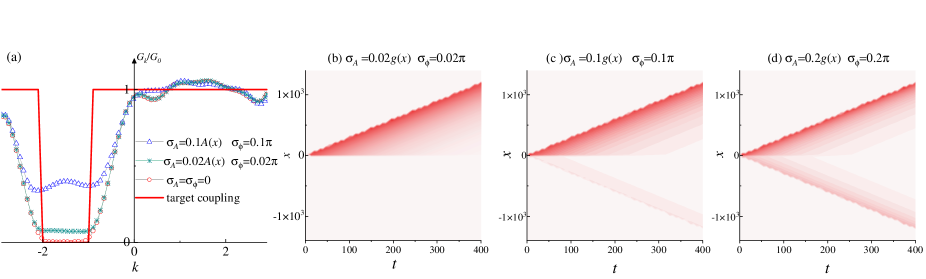
Figure S7: (a) The disorder averaged $k$-space coupling $G_{k}$ for the optimal sequence under different disorder strengths. (b, c, d) Time evolution of the chiral field distributions for various disorder strengths. The atomic frequency is fixed at $\omega_{q}=4.5$.

We now consider that the coupling strength at each point experiences disorders in both its amplitude and phase, i.e., $g(x_{i})\rightarrow[A(x_{i})+\delta A(x_{i})]\exp[{i\theta(x_{i})+i\delta\theta(x_{i})}].$ Both the amplitude and phase disorders are assumed to satisfy a Gaussian distribution centered around zero. The amplitude disorder widths $\sigma_{A}$ are proportional to the local strength $A(x_{i})$, while the phase disorder widths $\sigma_{\phi}$ are assumed identical for all the coupling points. We plot the disorder averaged $k$-space coupling function in Fig. S7(a). We find that the disorder does not affect the coupling strength too much for the modes outside the chiral regime. Inside the asymmetric band gap, the zero coupling will be lifted higher than zero with stronger disorder strengths.

To show how disorder disturbs the chiral emission, we numerically simulate disorder-averaged evolutions by defining the photonic field as

$$\bar{\Psi}_{\gamma}(x,t)=\frac{1}{N_{\text{dis}}}\sum_{n=1}^{N_{\text{dis}}}|\psi_{\gamma}(x,t)|^{2},\qquad\psi_{\gamma}(x,t)\propto\int_{-\infty}^{\infty}dkc_{k}(t)e^{-ikx}.$$ (S38)

In Fig. S7(b-d), we plot how the disorder-averaged field distribution $\psi_{\gamma}(x,t)$ changes with time in the presence of $\{\sigma_{A},\sigma_{\phi}\}$. When the coupling disorders are as strong as $\{\sigma_{A}=0.1g(x_{i}),\sigma_{\phi}=0.1\pi\}$, most of the photonic field still decays to the right of the waveguide. To evaluate the chiral behavior of our proposal, we define the chiral factor as

$$\beta_{\pm}=\frac{\Phi_{R(L)}}{\Phi_{R}+\Phi_{L}},$$ (S39)

$$\Phi_{R/L}=\frac{1}{N_{\text{dis}}}\sum_{n=1}^{N_{\text{dis}}}\left|\int_{0}^{\pm\infty}|\psi_{\gamma}(x^{\prime},t)|^{2}dx^{\prime}\right|,\quad t\rightarrow\infty.$$ (S40)

Employing the above methods and definitions, we plot Fig. 2 in the main text, and show that our proposal can chirally route photons in a broadband range even in the present of strong disorder.

References

- Scully and Zubairy (1997) M. O. Scully and M. S. Zubairy, Quantum Optics (Cambridge University Press, 1997).
- Agarwal (2012) G. S. Agarwal, Quantum Optics (Cambridge University Press, 2012).
- Kimble et al. (1977) H. J. Kimble, M. Dagenais, and L. Mandel, “Photon antibunching in resonance fluorescence,” Phys. Rev. Lett. 39, 691 (1977).
- Cohen-Tannoudji et al. (1998) C. Cohen-Tannoudji, J. Dupont-Roc, and G. Grynberg, Atom–Photon Interactions (Wiley, 1998).
- Gu et al. (2017) X. Gu, A. F. Kockum, A. Miranowicz, Y.-X. Liu, and F. Nori, “Microwave photonics with superconducting quantum circuits,” Phys. Rep. 718-719, 1 (2017).
- Kockum et al. (2019) A. F. Kockum, A. Miranowicz, S. De Liberato, S. Savasta, and F. Nori, “Ultrastrong coupling between light and matter,” Nat. Rev. Phys. 1, 19 (2019).
- Gustafsson et al. (2014) M. V. Gustafsson, T. Aref, A. F. Kockum, M. K. Ekstrom, G. Johansson, and P. Delsing, “Propagating phonons coupled to an artificial atom,” Science 346, 207 (2014).
- Kockum et al. (2014) A. F. Kockum, P. Delsing, and G. Johansson, “Designing frequency-dependent relaxation rates and Lamb shifts for a giant artificial atom,” Phys. Rev. A 90, 013837 (2014).
- Andersson et al. (2019) G. Andersson, B. Suri, L. Guo, T. Aref, and P. Delsing, “Non-exponential decay of a giant artificial atom,” Nat. Phys. 15, 1123 (2019).
- Zhao and Wang (2020) W. Zhao and Z. Wang, “Single-photon scattering and bound states in an atom-waveguide system with two or multiple coupling points,” Phys. Rev. A 101, 053855 (2020).
- Guo et al. (2020a) S. Guo, Y. Wang, T. Purdy, and J. Taylor, “Beyond spontaneous emission: Giant atom bounded in the continuum,” Phys. Rev. A 102, 033706 (2020a).
- Du et al. (2021) L. Du, M.-R. Cai, J.-H. Wu, Z.-H. Wang, and Y. Li, “Single-photon nonreciprocal excitation transfer with non-Markovian retarded effects,” Phys. Rev. A 103, 053701 (2021).
- Soro and Kockum (2022) A. Soro and A. F. Kockum, “Chiral quantum optics with giant atoms,” Phys. Rev. A 105, 023712 (2022).
- Yin et al. (2022) X.-L. Yin, Y.-H. Liu, J.-F. Huang, and J.-Q. Liao, “Single-photon scattering in a giant-molecule waveguide-qed system,” Phys. Rev. A 106, 013715 (2022).
- Du et al. (2022) L. Du, Y. Zhang, J.-H. Wu, A. F. Kockum, and Y. Li, “Giant atoms in a synthetic frequency dimension,” Phys. Rev. Lett. 128, 223602 (2022).
- Wang and Li (2022) X. Wang and H.-R. Li, “Chiral quantum network with giant atoms,” Quantum Sci. Technol. 7, 035007 (2022).
- Xiao et al. (2022) H. Xiao, L. Wang, Z.-H. Li, X. Chen, and L. Yuan, “Bound state in a giant atom-modulated resonators system,” npj Quantum Inf. 8, 80 (2022).
- Cheng et al. (2022) W. Cheng, Z. Wang, and Y.-x. Liu, “Topology and retardation effect of a giant atom in a topological waveguide,” Phys. Rev. A 106, 033522 (2022).
- Jia and Yu (2023) W. Z. Jia and M. T. Yu, “Atom-photon dressed states in a waveguide-qed system with multiple giant atoms coupled to a resonator-array waveguide,” arXiv:2304.02072 (2023).
- Santos and Bachelard (2023) A. C. Santos and R. Bachelard, “Generation of maximally entangled long-lived states with giant atoms in a waveguide,” Phys. Rev. Lett. 130, 053601 (2023).
- Kannan et al. (2020) B. Kannan et al., “Waveguide quantum electrodynamics with superconducting artificial giant atoms,” Nature (Lond.) 583, 775 (2020).
- Guo et al. (2017) L.-Z. Guo, A. Grimsmo, A. F. Kockum, M. Pletyukhov, and G. Johansson, “Giant acoustic atom: A single quantum system with a deterministic time delay,” Phys. Rev. A 95, 053821 (2017).
- Wang et al. (2021) X. Wang, T. Liu, A. F. Kockum, H.-R. Li, and F. Nori, “Tunable chiral bound states with giant atoms,” Phys. Rev. Lett. 126, 043602 (2021).
- Kockum et al. (2018) A. F. Kockum, G. Johansson, and F. Nori, “Decoherence-free interaction between giant atoms in waveguide quantum electrodynamics,” Phys. Rev. Lett. 120, 140404 (2018).
- Guo et al. (2020b) L.-Z. Guo, A. F. Kockum, F. Marquardt, and G. Johansson, “Oscillating bound states for a giant atom,” Phys. Rev. Res. 2, 043014 (2020b).
- Lim et al. (2022) K. Lim, W.-K. Mok, and L. Kwek, “Oscillating bound states in non-Markovian photonic lattices,” arXiv:2208.11097 (2022).
- Lodahl et al. (2015) P. Lodahl, S. Mahmoodian, and S. Stobbe, “Interfacing single photons and single quantum dots with photonic nanostructures,” Rev. Mod. Phys. 87, 347 (2015).
- Goban et al. (2015) A. Goban, C.-L. Hung, J. D. Hood, S.-P. Yu, J. A. Muniz, O. Painter, and H. J. Kimble, “Superradiance for atoms trapped along a photonic crystal waveguide,” Phys. Rev. Lett. 115, 063601 (2015).
- Roy et al. (2017) D. Roy, C. M. Wilson, and O. Firstenberg, “Colloquium: Strongly interacting photons in one-dimensional continuum,” Rev. Mod. Phys. 89, 021001 (2017).
- Chang et al. (2018) D. E. Chang, J. S. Douglas, A. González-Tudela, C.-L. Hung, and H. J. Kimble, “Colloquium: Quantum matter built from nanoscopic lattices of atoms and photons,” Rev. Mod. Phys. 90, 031002 (2018).
- Yu et al. (2019) S.-P. Yu, J. A. Muniz, C.-L. Hung, and H. J. Kimble, “Two-dimensional photonic crystals for engineering atom–light interactions,” Proc. Natl. Acad. Sci. U. S. A. 116, 12743 (2019).
- Scigliuzzo et al. (2022) M. Scigliuzzo, G. Calajò, F. Ciccarello, D. P. Lozano, A. Bengtsson, P. Scarlino, A. Wallraff, D. Chang, P. Delsing, and S. Gasparinetti, “Controlling atom-photon bound states in an array of Josephson-junction resonators,” Phys. Rev. X 12, 031036 (2022).
- Tang et al. (2022) J.-S. Tang, W. Nie, L. Tang, M.-Y. Chen, X. Su, Y.-Q. Lu, F. Nori, and K.-Y. Xia, “Nonreciprocal single-photon band structure,” Phys. Rev. Lett. 128, 203602 (2022).
- Kofman et al. (1994) A. Kofman, G. Kurizki, and B. Sherman, “Spontaneous and induced atomic decay in photonic band structures,” J. Mod. Opt. 41, 353 (1994).
- Smith et al. (2000) D. R. Smith, W. J. Padilla, D. C. Vier, S. C. Nemat-Nasser, and S. Schultz, “Composite medium with simultaneously negative permeability and permittivity,” Phys. Rev. Lett. 84, 4184 (2000).
- Lambropoulos et al. (2000) P. Lambropoulos, G. M. Nikolopoulos, T. R. Nielsen, and S. Bay, “Fundamental quantum optics in structured reservoirs,” Rep. Prog. Phys. 63, 455 (2000).
- Kafesaki et al. (2007) M. Kafesaki, I. Tsiapa, N. Katsarakis, T. Koschny, C. M. Soukoulis, and E. N. Economou, “Left-handed metamaterials: The fishnet structure and its variations,” Phys. Rev. B 75, 235114 (2007).
- Lu et al. (2014) D. Lu, J. J. Kan, E. E. Fullerton, and Z. Liu, “Enhancing spontaneous emission rates of molecules using nanopatterned multilayer hyperbolic metamaterials,” Nat. Nanotechnol. 9, 48 (2014).
- Indrajeet et al. (2020) S. Indrajeet, H. Wang, M. Hutchings, B. Taketani, F. K. Wilhelm, M. LaHaye, and B. Plourde, “Coupling a superconducting qubit to a left-handed metamaterial resonator,” Phys. Rev. Appl. 14, 064033 (2020).
- Stewart et al. (2020) M. Stewart, J. Kwon, A. Lanuza, and D. Schneble, “Dynamics of matter-wave quantum emitters in a structured vacuum,” Phys. Rev. Res. 2, 043307 (2020).
- John and Wang (1990) S. John and J. Wang, “Quantum electrodynamics near a photonic band gap: Photon bound states and dressed atoms,” Phys. Rev. Lett. 64, 2418 (1990).
- Le Kien et al. (2004) F. Le Kien, V. I. Balykin, and K. Hakuta, “Atom trap and waveguide using a two-color evanescent light field around a subwavelength-diameter optical fiber,” Phys. Rev. A 70, 063403 (2004).
- Le Kien et al. (2005) F. Le Kien, S. Dutta Gupta, V. I. Balykin, and K. Hakuta, “Spontaneous emission of a cesium atom near a nanofiber: Efficient coupling of light to guided modes,” Phys. Rev. A 72, 032509 (2005).
- Vetsch et al. (2010) E. Vetsch, D. Reitz, G. Sagué, R. Schmidt, S. T. Dawkins, and A. Rauschenbeutel, “Optical interface created by laser-cooled atoms trapped in the evanescent field surrounding an optical nanofiber,” Phys. Rev. Lett. 104, 203603 (2010).
- Hung et al. (2013) C. L. Hung, S. M. Meenehan, D. E. Chang, O. Painter, and H. J. Kimble, “Trapped atoms in one-dimensional photonic crystals,” New J. Phys. 15, 083026 (2013).
- Corzo et al. (2016) N. V. Corzo, B. Gouraud, A. Chandra, A. Goban, A. S. Sheremet, D. V. Kupriyanov, and J. Laurat, “Large Bragg reflection from one-dimensional chains of trapped atoms near a nanoscale waveguide,” Phys. Rev. Lett. 117, 133603 (2016).
- Liu and Houck (2017) Y. B. Liu and A. A. Houck, “Quantum electrodynamics near a photonic bandgap,” Nat. Phys. 13, 48 (2017).
- Zhou et al. (2008a) L. Zhou, Z. R. Gong, Y.-X. Liu, C. P. Sun, and F. Nori, “Controllable scattering of a single photon inside a one-dimensional resonator waveguide,” Phys. Rev. Lett. 101, 100501 (2008a).
- Liao et al. (2010) J.-Q. Liao, Z. R. Gong, L. Zhou, Y.-X. Liu, C. P. Sun, and F. Nori, “Controlling the transport of single photons by tuning the frequency of either one or two cavities in an array of coupled cavities,” Phys. Rev. A 81, 042304 (2010).
- Goban et al. (2014) A. Goban, C.-L. Hung, S.-P. Yu, J. Hood, J. Muniz, J. Lee, M. Martin, A. McClung, K. Choi, D. Chang, O. Painter, and H. Kimble, “Atom–light interactions in photonic crystals,” Nat. Commun. 5, 4808 (2014).
- Douglas et al. (2015) J. S. Douglas, H. Habibian, C.-L. Hung, A. V. Gorshkov, H. J. Kimble, and D. E. Chang, “Quantum many-body models with cold atoms coupled to photonic crystals,” Nat. Photon. 9, 326 (2015).
- Douglas et al. (2016) J. S. Douglas, T. Caneva, and D. E. Chang, “Photon molecules in atomic gases trapped near photonic crystal waveguides,” Phys. Rev. X 6, 031017 (2016).
- Hood et al. (2016) J. D. Hood, A. Goban, A. Asenjo-Garcia, M. Lu, S.-P. Yu, D. E. Chang, and H. J. Kimble, “Atom–atom interactions around the band edge of a photonic crystal waveguide,” Proc. Natl. Acad. Sci. U.S.A. 113, 10507 (2016).
- González-Tudela et al. (2015) A. González-Tudela, C.-L. Hung, D. E. Chang, J. I. Cirac, and H. J. Kimble, “Subwavelength vacuum lattices and atom–atom interactions in two-dimensional photonic crystals,” Nat. Photon. 9, 320 (2015).
- Munro et al. (2017) E. Munro, L. C. Kwek, and D. E. Chang, “Optical properties of an atomic ensemble coupled to a band edge of a photonic crystal waveguide,” New J. Phys. 19, 083018 (2017).
- Leonforte et al. (2021) L. Leonforte, A. Carollo, and F. Ciccarello, “Vacancy-like dressed states in topological waveguide QED,” Phys. Rev. Lett. 126, 063601 (2021).
- Mitsch et al. (2014) R. Mitsch, C. Sayrin, B. Albrecht, P. Schneeweiss, and A. Rauschenbeutel, “Quantum state-controlled directional spontaneous emission of photons into a nanophotonic waveguide,” Nat. Commun. 5, 6713 (2014).
- Bliokh et al. (2015a) K. Y. Bliokh, D. Smirnova, and F. Nori, “Quantum spin Hall effect of light,” Science 348, 1448 (2015a).
- Petersen et al. (2014) J. Petersen, J. Volz, and A. Rauschenbeutel, “Chiral nanophotonic waveguide interface based on spin-orbit interaction of light,” Science 346, 67 (2014).
- Young et al. (2015) A. Young, A. Thijssen, D. Beggs, P. Androvitsaneas, L. Kuipers, J. Rarity, S. Hughes, and R. Oulton, “Polarization Engineering in Photonic Crystal Waveguides for Spin-Photon Entanglers,” Phys. Rev. Lett. 115, 153901 (2015).
- Söllner et al. (2015) I. Söllner, S. Mahmoodian, S. L. Hansen, L. Midolo, A. Javadi, G. Kiršanskė, T. Pregnolato, H. El-Ella, E. H. Lee, J. D. Song, S. Stobbe, and P. Lodahl, “Deterministic photon–emitter coupling in chiral photonic circuits,” Nat. Nanotechnol. 10, 775 (2015).
- Bliokh et al. (2015b) K. Y. Bliokh, F. J. Rodríguez-Fortuño, F. Nori, and A. V. Zayats, “Spin–orbit interactions of light,” Nat. Photon. 9, 796 (2015b).
- Coles et al. (2016) R. J. Coles, D. M. Price, J. E. Dixon, B. Royall, E. Clarke, P. Kok, M. S. Skolnick, A. M. Fox, and M. N. Makhonin, “Chirality of nanophotonic waveguide with embedded quantum emitter for unidirectional spin transfer,” Nat. Commun. 7 (2016).
- Lodahl et al. (2017) P. Lodahl, S. Mahmoodian, S. Stobbe, A. Rauschenbeutel, P. Schneeweiss, J. Volz, H. Pichler, and P. Zoller, “Chiral quantum optics,” Nature (London) 541, 473 (2017).
- Patterson et al. (2009) M. Patterson, S. Hughes, S. Combrié, N.-V.-Q. Tran, A. De Rossi, R. Gabet, and Y. Jaouën, “Disorder-induced coherent scattering in slow-light photonic crystal waveguides,” Phys. Rev. Lett. 102, 253903 (2009).
- García et al. (2010) P. D. García, S. Smolka, S. Stobbe, and P. Lodahl, “Density of states controls Anderson localization in disordered photonic crystal waveguides,” Phys. Rev. B 82, 165103 (2010).
- Lang et al. (2015) B. Lang, D. M. Beggs, A. B. Young, J. G. Rarity, and R. Oulton, “Stability of polarization singularities in disordered photonic crystal waveguides,” Phys. Rev. A 92, 063819 (2015).
- Mann et al. (2015) N. Mann, A. Javadi, P. D. García, P. Lodahl, and S. Hughes, “Theory and experiments of disorder-induced resonance shifts and mode-edge broadening in deliberately disordered photonic crystal waveguides,” Phys. Rev. A 92, 023849 (2015).
- (69) See Supplementary Material at http://xxx for detailed derivations of our main results.
- Zhou et al. (2008b) L. Zhou, H. Dong, Y.-X. Liu, C. P. Sun, and F. Nori, “Quantum supercavity with atomic mirrors,” Phys. Rev. A 78, 063827 (2008b).
- González-Tudela and Cirac (2017) A. González-Tudela and J. I. Cirac, “Markovian and non-Markovian dynamics of quantum emitters coupled to two-dimensional structured reservoirs,” Phys. Rev. A 96, 043811 (2017).
- González-Tudela and Cirac (2017) A. González-Tudela and J. I. Cirac, “Quantum emitters in two-dimensional structured reservoirs in the nonperturbative regime,” Phys. Rev. Lett. 119, 143602 (2017).
- Bello et al. (2019) M. Bello, G. Platero, J. I. Cirac, and A. González-Tudela, “Unconventional quantum optics in topological waveguide QED,” Sci. Adv. 5, eaaw0297 (2019).
- Kim et al. (2021) E. Kim, X. Zhang, V. S. Ferreira, J. Banker, J. K. Iverson, A. Sipahigil, M. Bello, A. González-Tudela, M. Mirhosseini, and O. Painter, “Quantum electrodynamics in a topological waveguide,” Phys. Rev. X 11, 011015 (2021).
- Chen et al. (2014) Y. Chen et al., “Qubit architecture with high coherence and fast tunable coupling,” Phys. Rev. Lett. 113, 220502 (2014).
- Wulschner et al. (2016) F. Wulschner et al., “Tunable coupling of transmission-line microwave resonators mediated by an rf SQUID,” EPJ Quantum Technol. 3, 10 (2016).
- McKay et al. (2016) D. C. McKay, S. Filipp, A. Mezzacapo, E. Magesan, J. M. Chow, and J. M. Gambetta, “Universal gate for fixed-frequency qubits via a tunable bus,” Phys. Rev. Appl. 6, 064007 (2016).
- Roushan et al. (2017) P. Roushan et al., “Chiral ground-state currents of interacting photons in a synthetic magnetic field,” Nat. Phys. 13, 146 (2017).
- Kounalakis et al. (2018) M. Kounalakis, C. Dickel, A. Bruno, N. K. Langford, and G. A. Steele, “Tuneable hopping and nonlinear cross-Kerr interactions in a high-coherence superconducting circuit,” npj Quantum Inf. 4, 38 (2018).
- Yan et al. (2018) F. Yan, P. Krantz, Y. Sung, M. Kjaergaard, D. L. Campbell, T. P. Orlando, S. Gustavsson, and W. D. Oliver, “Tunable coupling scheme for implementing high-fidelity two-qubit gates,” Phys. Rev. Appl. 10, 054062 (2018).
- Joshi et al. (2022) C. Joshi, F. Yang, and M. Mirhosseini, “Resonance fluorescence of a chiral artificial atom,” arXiv:2212.11400 (2022).
- Ramos et al. (2016) T. Ramos, B. Vermersch, P. Hauke, H. Pichler, and P. Zoller, “Non-Markovian dynamics in chiral quantum networks with spins and photons,” Phys. Rev. A 93, 062104 (2016).
- González-Tudela et al. (2019) A. González-Tudela, C. S. Muñoz, and J. I. Cirac, “Engineering and harnessing giant atoms in high-dimensional baths: A proposal for implementation with cold atoms,” Phys. Rev. Lett. 122, 203603 (2019).
- Chen et al. (2022) Y.-T. Chen, L. Du, L. Guo, Z. Wang, Y. Zhang, Y. Li, and J.-H. Wu, “Nonreciprocal and chiral single-photon scattering for giant atoms,” Communications Physics 5, 215 (2022).
- Caloz et al. (2018) C. Caloz, A. Alù, S. Tretyakov, D. Sounas, K. Achouri, and Z. Deck-Léger, “Electromagnetic nonreciprocity,” Phys. Rev. Appl. 10, 047001 (2018).
- Zhang et al. (2021) Y.-X. Zhang, C. Carceller, M. Kjaergaard, and A. S. Sørensen, “Charge-noise insensitive chiral photonic interface for waveguide circuit QED,” Phys. Rev. Lett. 127, 233601 (2021).
- Gheeraert et al. (2020) N. Gheeraert, S. Kono, and Y. Nakamura, “Programmable directional emitter and receiver of itinerant microwave photons in a waveguide,” Phys. Rev. A 102, 053720 (2020).
- Kannan et al. (2022) B. Kannan et al., “On-demand directional microwave photon emission using waveguide quantum electrodynamics,” arXiv:2203.01430 (2022).
- Shi et al. (2016) T. Shi, Y.-H. Wu, A. González-Tudela, and J. I. Cirac, “Bound states in Boson impurity models,” Phys. Rev. X 6, 021027 (2016).
- Mahmoodian et al. (2018) S. Mahmoodian, M. Čepulkovskis, S. Das, P. Lodahl, K. Hammerer, and A. S. Sørensen, “Strongly correlated photon transport in waveguide quantum electrodynamics with weakly coupled emitters,” Phys. Rev. Lett. 121, 143601 (2018).
- Mahmoodian et al. (2020) S. Mahmoodian, G. Calajó, D. E. Chang, K. Hammerer, and A. S. Sørensen, “Dynamics of many-body photon bound states in chiral waveguide QED,” Phys. Rev. X 10, 031011 (2020).
- Kusmierek et al. (2022) K. Kusmierek, S. Mahmoodian, M. Cordier, J. Hinney, A. Rauschenbeutel, M. Schemmer, P. Schneeweiss, J. Volz, and K. Hammerer, “Higher-order mean-field theory of chiral waveguide QED,” arXiv:2207.10439 (2022).
- Johansson et al. (2012) J. R. Johansson, P. D. Nation, and F. Nori, “Qutip: An open-source Python framework for the dynamics of open quantum systems,” Comput. Phys. Commun. 183, 1760 (2012).
- Johansson et al. (2013) J. R. Johansson, P. D. Nation, and F. Nori, “Qutip 2: A Python framework for the dynamics of open quantum systems,” Comput. Phys. Commun. 184, 1234 (2013).

References

- Guo et al. (2020) L.-Z. Guo, A. F. Kockum, F. Marquardt, and G. Johansson, “Oscillating bound states for a giant atom,” Phys. Rev. Res. 2, 043014 (2020).
- Koch et al. (2007) J. Koch, T. M. Yu, J. Gambetta, A. A. Houck, D. I. Schuster, J. Majer, A. Blais, M. H. Devoret, S. M. Girvin, and R. J. Schoelkopf, “Charge-insensitive qubit design derived from the Cooper pair box,” Phys. Rev. A 76, 042319 (2007).
- (3) J. Q. You, X. Hu, S. Ashhab, and F. Nori, “Low-decoherence flux qubit,” Phys. Rev. B , 140515.
- Gu et al. (2017) X. Gu, A. F. Kockum, A. Miranowicz, Y.-X. Liu, and F. Nori, “Microwave photonics with superconducting quantum circuits,” Phys. Rep. 718-719, 1 (2017).
- Chen et al. (2014) Y. Chen et al., “Qubit architecture with high coherence and fast tunable coupling,” Phys. Rev. Lett. 113, 220502 (2014).
- Wulschner et al. (2016) F. Wulschner et al., “Tunable coupling of transmission-line microwave resonators mediated by an rf SQUID,” EPJ Quantum Technol. 3, 10 (2016).
- McKay et al. (2016) D. C. McKay, S. Filipp, A. Mezzacapo, E. Magesan, J. M. Chow, and J. M. Gambetta, “Universal gate for fixed-frequency qubits via a tunable bus,” Phys. Rev. Appl. 6, 064007 (2016).
- Roushan et al. (2017) P. Roushan et al., “Chiral ground-state currents of interacting photons in a synthetic magnetic field,” Nat. Phys. 13, 146 (2017).
- Kounalakis et al. (2018) M. Kounalakis, C. Dickel, A. Bruno, N. K. Langford, and G. A. Steele, “Tuneable hopping and nonlinear cross-Kerr interactions in a high-coherence superconducting circuit,” npj Quantum Inf. 4, 38 (2018).
- Yan et al. (2018) F. Yan, P. Krantz, Y. Sung, M. Kjaergaard, D. L. Campbell, T. P. Orlando, S. Gustavsson, and W. D. Oliver, “Tunable coupling scheme for implementing high-fidelity two-qubit gates,” Phys. Rev. Appl. 10, 054062 (2018).
- Joshi et al. (2022) C. Joshi, F. Yang, and M. Mirhosseini, “Resonance fluorescence of a chiral artificial atom,” arXiv:2212.11400 (2022).
- Wang and Li (2022) X. Wang and H.-R. Li, “Chiral quantum network with giant atoms,” Quantum Sci. Technol. 7, 035007 (2022).
- Ramos et al. (2016) T. Ramos, B. Vermersch, P. Hauke, H. Pichler, and P. Zoller, “Non-Markovian dynamics in chiral quantum networks with spins and photons,” Phys. Rev. A 93, 062104 (2016).
- Cohen-Tannoudji et al. (1998) C. Cohen-Tannoudji, J. Dupont-Roc, and G. Grynberg, Atom–Photon Interactions (Wiley, 1998).
- James and Jerke (2007) D. F. James and J. Jerke, “Effective hamiltonian theory and its applications in quantum information,” Can. J. Phys. 85, 625 (2007).