GMValuator: Similarity-based Data Valuation for Generative Models
Abstract
Data valuation plays a crucial role in machine learning. Existing data valuation methods have primarily focused on discriminative models, neglecting generative models that have recently gained considerable attention. A very few existing attempts of data valuation method designed for deep generative models either concentrates on specific models or lacks robustness in their outcomes. Moreover, efficiency still reveals vulnerable shortcomings. To bridge the gaps, we formulate the data valuation problem in generative models from a similarity-matching perspective. Specifically, we introduce Generative Model Valuator (GMValuator), the first training-free and model-agnostic approach to provide data valuation for generation tasks. It empowers efficient data valuation through our innovatively similarity matching module, calibrates biased contribution by incorporating image quality assessment, and attributes credits to all training samples based on their contributions to the generated samples. Additionally, we introduce four evaluation criteria for assessing data valuation methods in generative models, aligning with principles of plausibility and truthfulness. GMValuator is extensively evaluated on various datasets and generative architectures to demonstrate its effectiveness.
I Introduction
As the driving force behind modern artificial intelligence, particularly deep learning [1], a substantial volume of data is indispensable for effective machine learning. On one hand, informative data samples that are relevant to the task at hand play a critical role in the training process. On the other hand, due to data privacy concerns, personal data is safeguarded by various regulations, including the General Data Protection Regulation (GDPR) [2], and has become a valuable asset. Consequently, data valuation has garnered significant attention from both academic and industrial sectors in recent times.
The intricate relationship between data and model parameters presents a significant challenge in contribution measurement of each training sample, thus making data valuation a difficult task. Most of the existing data valuation studies focus on supervised learning for discriminative models (e.g., classification and regression). These methods can be categorized as: (1) Metric-based methods: methods such as Shapley Value (SV) and Banzhaf Index(BI) [3, 4] provide the assessment of data value by calculating marginal contribution on performance metrics (e.g., accuracy or loss) through retraining the model111Exception for KNN-Shap [5]. (2) Influence-based methods: this line of methods measures data value by evaluating influence on model parameters of data points [6, 7]. (3) Data-driven methods: These techniques avoid retraining by leveraging data characteristics (like data diversity, generalization bound estimation, class-wise distance), though generally necessitate data labels. [8, 9, 10].
Data valuation in the context of generative models has NOT been well-investigated in the current literature. Moreover, there exist significant challenges in directly adapting the aforementioned data valuation methods for discriminative models listed to generative models: Firstly, the challenge of applying metric-based methods arises from lacking robust performance metrics in generative models, in contrast to the existance of commonly used metrics (e.g., accuracy or loss) in discriminative models. In addition, the expensive cost of retrain requirements is another obstacle to use metric-based methods. Secondly, influence-based methods may not perform well on non-convex objective function of generative models [11]. Besides, estimating influence function in deep generative model is expensive, as it requires computing (or approximation) inverse Hessian. Thirdly, for data-driven methods, they mainly focus on supervised learning, requires knowing data labels to quantify data values.
To the best of our knowledge, limited studies have explored model-dependent data evaluation using influence functions for specific generative models. IF4GAN [12] consider multiple evaluation metrics, such as log-likelihood, inception score (IS), and Frechet inception distance (FID) [13] to identify the most responsible training samples for the overall performance of generative adversarial networks (GAN)-based models. However, the selection of appropriate metrics is critical, as the results are inconsistent across metrics. VAE-TracIn [14] finds the most significant contributors for generating a particular generated sample for Variational Autoencoders (VAE) using influence function. However, viable Hessian estimation in influence function calculations incur high computational costs and this method cannot be easily generalized to other generative models.
Considering the challenges posed by the selection of performance metrics and computational efficiency, as well as the need for broader applicability across various generative models, we aim to propose a unified and efficient data valuation method. We expect the unified method to satisfy the following key properties: 1) Model-agnostic: the method should be versatile, capable of being employed across diverse generative model architectures and algorithms, regardless of specific design choices; 2) Computation Efficiency: the method does not require retraining the model and minimize computational overhead while maintaining a satisfactory level of accuracy and reliability in evaluating the value of data points; 3) Plausibility: the method should evaluate the value of data based on its alignment with human prior knowledge on the task, enhancing its credibility and reliability; 4) Truthfulness: the method should strive to provide an unbiased and accurate assessment of the value associated with individual data points. To meet the design purposes, we propose a similarity-based data valuation approach for the generative model, called GMValuator, which is model-agnostic and efficient.
In summary, our work here provides the following specific novel contributions:
-
•
To the best of our knowledge, GMValuator is the first modal-agnostic and retraining-free data valuation method for generative models.
-
•
We formulate data valuation for generative models as an efficient similarity-matching problem. We further eliminate the biased contribution measurement by introducing image quality assessment for calibration.
-
•
We propose four evaluation methods to assess the truthfulness of data valuation and evaluate GMValuator on different datasets and deep generative models to verify its validity.
II Related Work
II-A Data Valuation
There are three lines of methods on data valuation: metric-based methods, influence-based methods and data-driven methods. In terms of metric-based methods, the commonly-used approach is to calculate its marginal contribution (MC) based on performance metrics (e.g., accuracy, loss). As the basic method depending on performance metrics for data valuation, LOO (Leave-One-Out) [15] is used to evaluate the value of training sample by observational change of model performance when leaving out that data point from the training dataset. To overcome inaccuracy and strict desirability of LOO, SV [3] and BI [4] originated from Cooperative Game Theory are widely used to measure the contribution of data [6, 16]. Considering the joining sequence of each training data point, SV needs to calculate the marginal performance of all possible subsets in which the time complexity is exponential. Despite the introduction of techniques such as Monte-Carlo and gradient-based methods, as well as others proposed in the literature, to approximate data significance value (SV) is computationally expensive and it typically require retraining [3, 5]. The computational cost and needs for unconventional performance metrics presents difficulties in adapting the methods to generative models. As for influence-based methods, they evaluate the influence of data points on model parameters by computing the inverse Hessian for data valuation [5, 17, 18]. Due to the high computational cost, some approximation methods have also been proposed [19]. In addition, the use of influence function for data valuation is not limited to discriminative models, but can also be applied to specific generative models such as GAN and VAE [12, 14]. When it comes to data-driven methods, most of them are training-free methods that focus on the data itself [8, 9, 10].
II-B Generative Model
Generative models are a type of unsupervised learning that can learn data distributions. Recently, there has been significant interest in combining generative models with neural networks to create Deep Generative Models, which are particularly useful for complex, high-dimensional data distributions. They can approximate the likelihood of each observation and generate new synthetic data by incorporating variations. Variational auto-encoders (VAEs) [20] optimize the log-likelihood of data by maximizing the evidence lower bound (ELBO), while generative adversarial networks (GANs) [21, 22] involves a generator and discriminator that compete with each other, resulting in strong image generation. Recently proposed diffusion models [23, 24] add Gaussian noise to training data and learn to recover the original data. These models use variational inference and have a fixed procedure with a high-dimensional latent space.
III Motivation and Problem Formulation
In this section, we present the background and motivation behind our proposed method GMValuator, which formulates the data valuation for generative models as a similarity matching problem.
III-A Motivation
Let denote the training dataset for generative model training, in which and is regarded as the size of data. Let present the learning algorithm of generative models (e.g., Generative Adversarial Network (GAN), Variational Autoencoder (VAE), Diffusion Model). The primary goal of generative models is to generate synthetic data samples that are closely similar to the real data. Thus, the core of the generative model is an intractable probability distribution learning process to train a generator , that maps each sample sampled from the noise distribution to a sample in estimated distribution while minimizing the discrepancy () between the estimated distribution and real data distribution :
It’s important to understand the significance of each training data point in relation to the generated data. The objective function can be calculated using likelihood in (1), where qualifies the similarity between and . The value of should be high as looks like the sampling data , by maximizing the likelihood .
| (1) |
Thus, generated data should exhibit a higher degree of similarity to the data points used to train the generator than the ones not used for training, despite originating from a similar distribution.
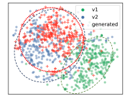
Therefore, we put forth the plausible assumption that the similarity between training data and generated data characterizes the contribution of the training data to the generated data for any given model. We support the assumption by partitioning a class of CIFAR-10 (the class is plane here) into two non-overlapped subsets, denoted as and .222In practice, we perform T-SNE first to randomly split the non-overlapped samples from the embedding space. Next, we keep as non-training data and use as training data to train a BigGAN [25] to generate dataset . If our assumption holds, the generated data will be more similar to the training data . As presented in the T-SNE plot (Figure 1), the generated data demonstrate a more substantial overlap in the shared feature space with the training dataset than the non-training ones .333Quantitative statistical testing is provided in Appendix. This observation motivates us to address the data valuation for the generative model from a similarity-matching perspective.
It’s worth noting that concurrent to our research, LAVA [10] also proposes the utilization of a similarity metric, specifically the class-wise Wasserstein distance between the training and validation sets, to evaluate data value. However, their emphasis lies in classification tasks and theoretical analysis, whereas our work contributes practical algorithms tailored for generative models.
III-B Problem Formulation and Challenges
The primary objective of our research is to tackle the issue of data valuation in generative models using black-box access. In essence, given a fixed set of data samples with a size of generated from the trained deep generative model , our aim is to determine the value associated with each data point for in the deduplicated training dataset, which contributes to the generated dataset. We denote the value for training data as in the rest of the paper for simplicity.
Following the motivation stated in Sec. III-A, should be a functions of the distance between the data points. We denote the distance between training data and generated data as , for and . The contribution score of to is denoted as , which is inversely proportional to distance since maximizing the log-likelihood of a generative model is equivalent to minimizing the dissimilarity of real and generated data distribution. To link the dissmilarity to likelihood, we choose to likelihood, and define as follows:
| (2) |
Therefore, an intuitive definition for the value of data can be written as
| (3) |
The high-value data will achieve a smaller distance to the target distributions, thus, a better approximation. Therefore, data valuation in the above problem formulation contains two steps: Step 1, calculating all of the score value ; Step 2, mapping the contribution from training data to generative data based on the scores .
However, there are several open questions and challenges in performing the above two steps for calculating Eq. (3):
Challenge 1: Efficiency. In step 1, considering training samples and generated samples, where represents the complexity of the selected pair-wise distance calculation, the total complexity of this step amounts to . In practical scenarios with large training datasets (e.g., ), the computation cost for becomes prohibitively expensive. Additionally, fitting
such a large collection of high-dimensional data for distance calculation can pose significance challenges in system memory.
Challenge 2: Contribution plausibility. To ensure that a training data point contributes more if it is similar to high-quality generated data and less if it is similar to low-quality generated data, the contribution scores should be adjusted based on the quality of the generated data.
Challenge 3: Non-zero scores. In practical scenarios, the distance between training data and the least similar generated data is not infinite, which may result in false non-zero contribution scores. With a large dataset size, the accumulation of these noisy scores yield biased data valuation.
In light of this, we present a novel and efficient data valuation approach suitable for agnostic generative models, termed as GMValuator as elaborated in Section IV.
IV The Proposed Data Valuation Methods
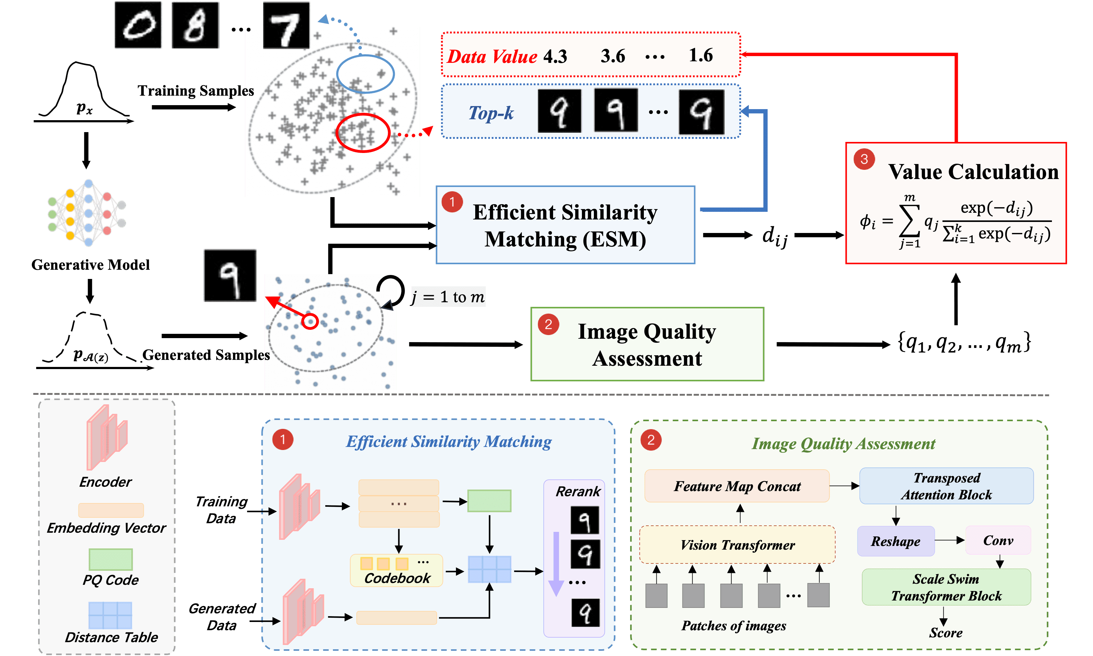
The crucial idea behind GMValuator is to transform the data valuation problem into a similarity matching problem between generated and training data. The overview of GMValuator is presented in Figure 2. To tackle challenge 1, we propose to employ efficient similarity matching (ESM), where each generated data point can be linked to multiple contributors from the training dataset (Section IV-A), where each generated data firstly link with top contributors via recall phase and then re-rank by a refined similarity for effectiveness. After that, the image quality of the generated sample is assessed to weight the valuation (Sec. IV-B). Finally, the value computation function combines both the quality score and the image-space similarity score to measure the value of the training data (Sec. IV-C).
IV-A Efficient Similarity Matching
Considering the complexity of calculating , we formulate it as an ESM problem between generative data and training data. Each generative data point is matched to several training data points based on their similarity. We denote as the subset of training data that contains the most similar data points. Here, represents the similarity-matching strategy, encompassing the recall and re-ranking phases, which will be introduced subsequently.
Recall Phase: The main aim of the recall phase is to rapidly identify a subset of training samples that are similar to a generated sample. To achieve this, an initial step involves encoding all original training images and generated samples from the image space to a lower-dimensional embedding space using a pre-trained encoder (such as VGG-16) to reduce computational complexity. Subsequently, the technique of Product Quantization (PQ) [26] is employed to further decrease the computational burden. Specifically, PQ divides embedding vectors into subvectors and independently quantizes each subvector through -means clustering. This process generates compact PQ codes that serve as representations of the original vectors. This representation significantly reduces the vector sizes, allowing for efficient estimation of Euclidean Distance between two samples. By incorporating the recall method into the similarity matching process, the computational complexity is lowered from to , where and . Consequently, generated images can quickly identify their top- most similar training data points.
Re-Ranking Phase: Following the PQ-based efficient recall process in GMValuator, we further improve the precision of the results by utilizing perceptual similarity [27] for precision ranking. Once we have extracted perceptual features from the top recalled training samples, we proceed to calculate the distance for each pair of items. To obtain precise distance measurements based on their perceptual content, we propose to use Learned Perceptual Image Patch Similarity (LPIPS) [28] or DreamSim [27] as the distance measurement to gain insights into the perceptual dissimilarity between the generated sample and different training samples. These metric enable us to precisely measure the most significant contributors according to their perceived similarity, more importantly, the obtained distance will be employed to compute data valuation in Eq. (4). We do not use Wasserstein distance as it is more proper to measure dissimilarity between two probability distributions rather than a pair of image instances.
IV-B Image Quality Assessment
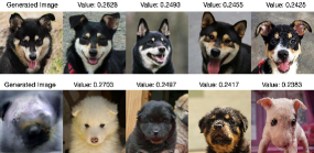
To tackle challenge 2, we have to establish a connection between the quality of the generated sample that the training samples contribute to and the contribution score. This is necessary before assigning contribution scores to the ranked training samples for the generated sample. For low-quality generated samples , we expect their total contribution score from contributors to be lower compared to high-quality samples , namely . This motivation arises from the observations in Figure 3, where the first and second rows show generated samples using from a normal distribution and uniform distribution, respectively. The values denoted in Figure 3 directly employs Eq (2), so we have for . The real samples are noticeably dissimilar to the generated data, yet they are still assigned a high value. Therefore, we propose to calibrate the contribution scores with generated data quality. Specifically, we obtain a comprehensive quality score for each generated image integrate using MANIQA [29] model into our evaluation process. A higher indicate better data quality. This score of MANIQA considers various factors such as sharpness, color accuracy, composition, and overall visual appeal. Incorporating the image quality evaluation provided by MANIQA allows us to more accurately assess the generated images and take into account their perceptual fidelity and aesthetic qualities.
Input: Training dataset , a well-trained
model , random distribution .
Output: Generated dataset , the value of training data
points
IV-C Value Calculation
Finally, we utilize the image quality to calibrate the contribution scores. Notably, during the recall phase of similarity matching, we select the top contributors for the generated data . Consequently, we only consider the contribution score between and by setting for . This strategy addresses challenge 3 by assigning zero scores to irrelevant samples, effectively reducing bias and noise in value estimation when dealing with a large . Hence, we define the contribution score function of each training data point for a specific synthetic data point as follows:
| (4) |
which is used to give different scores to training data points according to their ranking distance. The final data value is obtained by plugging Eq. (4) into Eq. (3).
V Experiments
Given the absence of a definitive benchmark to evaluate data valuation methods in the context of generative models, we propose to evaluate the truthfulness of data valuation outcomes through the examination of four criteria (C):
-
•
C1: Identical Class Test. Following the concept of an identical class [30], we posit that the most significant contributors among the training samples should belong to the same class as the generated sample produced by a well-trained generative model, which is also used for evaluation in VAE-TrancIn [14].
-
•
C2: Identical Attributes Test. We consider the attributes of samples as the ground truth to examine the most significant contributors by our approach. We examine the overlap level of attributes (i.e., the number of identical attributes) between the most valuable training samples with the generated sample
-
•
C3: Data Cleansing. Under the assumption, noisy training data samples can be identified as low-value training data. To evaluate the performance of data valuation approaches, we consider the value level of noisy data samples as the performance metric across various approaches.
-
•
C4: Efficiency. As an efficient training-free approach, GMValuator should measure the data value in a limited time and be much more efficient than the previous work while obtaining truthful results.
| Dataset | Network | |||
| C1 | MNIST, CIFAR-10 | GAN, Diffusion, -VAE | ||
| C2 | CelebA | Diffusion-StyleGAN | ||
| AFHQ | StyleGAN | |||
| C3 | Noise MNIST | DCGAN | ||
| C4: Hardware Evironment | ||||
| CPU | One RTX 3080 (10GB) GPU | |||
| GPU |
|
|||
Experiment Setup. Our experiment settings are listed in in Table I. Particularly, we consider different type of generative models, including GAN based models, -VAE [31], and diffusion models [32, 33]. The generation tasks are conducted on benchmark datasets (i.e., MNIST [34] and CIFAR [35]), face recognition dataset (i.e., CelebA [36]) and high-resolution image dataset with size 512 512, and 1024 1024 (i.e., AFHQ [37], FFHQ [38]).
Note that GMValuator is a model agnostic method. To showcase its efficacy, we compare it with two baseline methods: VAE-TracIn [14] and IF4GAN [12]. VAE-TracIn identifies the most significant contributors for a generated sample, which is same to the similarity matching process of GMValuator (Sec. IV-A). Thus, we compare GMValuator with VAE-TracIn in Sec. V-A and Sec. V-B. IF4GAN finds the high-valued training samples for generative model training, which we regard it as baseline method in section V-C. We also examine our approach using DreamSim, LPIPS and -distance in the re-ranking phase, referred to as GMValuator (DreamSim), GMValuator (LPIPS) and GMValuator (-distance) respectively, while the GMValuator without the re-ranking phase is referred to as GMValuator (No-Rerank).
V-A Identical Class Test (C1)
Methodology. In this subsection, we follow setup of VAE-TracIn [14] by training separate -VAE models on MNIST [35], CIFAR [34]. We then attribute the most significant contributors by VAE-TracIn and our approach over generated samples. By the concept of identical class test, we expects a perfect data valuation approach should indicate training data in the same subclass of the generated sample contribute more to . We examine GMValuator (DreamSim), GMValuator (LPIPS), GMValuator (-distance) and GMValuator (No-Rerank) separately. Apart from that, due to our method is model-agnostic, we also valid our method on GAN, Diffusion model, which are other kinds of generative models.
Results. For a given generated data, we examine the class(es) of is top contributors in the training data. We count the number of training samples in the top contributors, which has the identical class as the generated data. The identical class ratio . We report the averaged over the generated datasets (the data size =100) on different choices of in Table II. GMValuator has the most contributors that belong to the same class with the generated sample among on MNIST and CIFAR-10, while GMValuator (DreamSim) has the best performance. The results for CIFAR-10 using VAE-TracIn is extremely bad. This could be attributed to underfitting, as the authors mentioned in their study [14], training a good -VAE model on CIFAR-10 is challenging. The results of other diverse generative models are show in Table VI in appendix.
| MNIST (%) | =30 | =50 | =100 |
| VAE-TracIn | 72.00 | 71.11 | 68.58 |
| GMValuator (No-Rerank) | 86.41 | 85.13 | 85.95 |
| GMValuator (-distance) | 87.76 | 86.95 | 85.92 |
| GMValuator (LPIPS) | 88.78 | 88.19 | 86.69 |
| GMValuator (DreamSim) | 88.78 | 88.05 | 86.84 |
| CIFAR-10 (%) | =30 | =50 | =100 |
| VAE-TracIn | 6.28 | 3.77 | 1.88 |
| GMValuator (No-Rerank) | 72.66 | 72.25 | 70.71 |
| GMValuator (-distance) | 72.66 | 72.25 | 70.71 |
| GMValuator (LPIPS) | 72.60 | 71.75 | 70.84 |
| GMValuator (DreamSim) | 77.94 | 76.41 | 73.47 |
V-B Identical Attributes Test (C2)
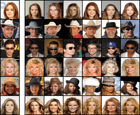
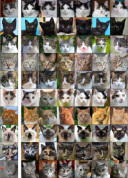
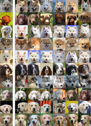
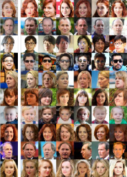
Methodology. By regarding some attributes of images as the ground-truth, we assume that the most significant contributors should have the similar attributes to the generated sample. We train Diffusion-StyleGAN [33] on CelebA, and leverage our approach to identify the most significant contributors in training samples, and use some some attributes including glasses, hair, hat, sex as the ground-truth, to check the correctness of our approach for identifying the most significant contributors for a generated sample. We also examine this on AFHQ, FFHQ dataset by StyleGAN [37].
Results. The results in Table III indicates that GMValuator can find the most significant contributors with the same attributes to the generated sample. Besides, using DreamSim in similarity re-ranking phase obtains the best performance over these three attributes. We also visualize some visible results in Figure 4 on CelebA and Figure 6 on AFHQ, FFHQ in Appendix. As we can see, the most significant contributors have the similar attributes (e.g., skin color, hair) to the generated sample.
| Top K contributors: | =5 | =10 | =15 |
| Attribute: Hat (%) | |||
| GMValuator (No-Rerank) | 92.52 | 92.12 | 91.92 |
| GMValuator (-distance) | 90.91 | 89.90 | 89.83 |
| GMValuator (LPIPS) | 96.77 | 96.57 | 96.90 |
| GMValuator (DreamSim) | 97.78 | 97.07 | 96.90 |
| Attribute: Gender (%) | |||
| GMValuator (No-Rerank) | 75.15 | 75.25 | 75.82 |
| GMValuator (-distance) | 63.64 | 61.01 | 60.00 |
| GMValuator (LPIPS) | 97.98 | 97.48 | 97.37 |
| GMValuator (DreamSim) | 99.19 | 98.99 | 98.79 |
| Attribute: Eyeglasses (%) | |||
| GMValuator (No-Rerank) | 91.52 | 91.52 | 91.45 |
| GMValuator (-distance) | 94.95 | 94.65 | 93.80 |
| GMValuator (LPIPS) | 94.95 | 94.65 | 93.80 |
| GMValuator (DreamSim) | 96.77 | 96.26 | 95.96 |
V-C Data Cleaning (C3)
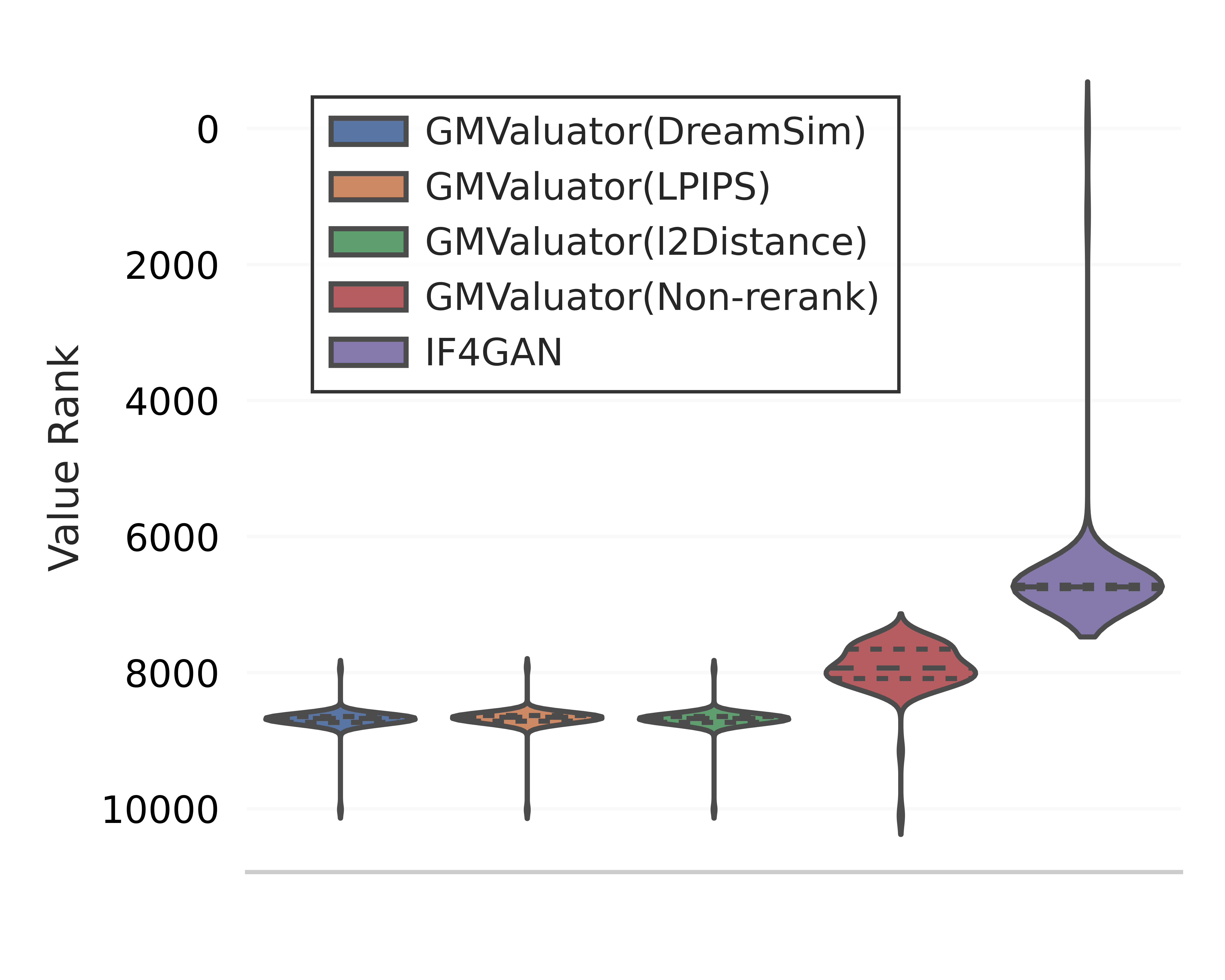
Methodology In this experiment, we introduce 100 noisy images into the MNIST dataset to create a new corrupted training dataset and each noisy image is generated by adding Gaussian noise to the clean data. These contaminated samples can diminish the performance of generative models, and as a result, they are anticipated to possess lower values compared to the rest of the training dataset. Our objective is to assess the performance of both GMValuator and its baseline method, IF4GAN [12], by analyzing the value rankings of noisy samples. An effective approach should place noisy data in lower positions within the value ranking. We conducted this evaluation using 10,000 generated images and referred to the study [12] for the baseline method (IF4GAN).
Results. The results are depicted in Figure 5 demonstrate that the values of all noisy training samples, as calculated by GMValuator, are lower compared to the values calculated by IF4GAN. This observation suggests that the performance of GMValuator is significantly better than that of IF4GAN. Besides, the performance of GMValuator with re-ranking phase is better than GMValuator (No-rerank).
V-D Efficiency (C4)
Methodology. We thoroughly evaluate and compare the efficiency of our approach against existing data valuation methods for generative models discussed above: VAE-TracIn and IF4GAN. Specifically, we measure the attribute time for one generated sample on an average of 100 test samples using both VAE-TracIn and our proposed approach on MNIST and CIFAR-10. Additionally, under the same setting in C3, we assess the data valuation time when utilizing IF4GAN and our approaches on noise MNIST which we mentioned in C3.
Results. The average time taken to attribute the most significant contributors for one generated sample is calculated and compared with the baseline method (VAE-TracIn), as demonstrated in Table IV. Our approaches are all greatly more efficient than the baseline methods on both datasets. When it comes to data valuation for GAN, GMValuator (No-rerank) and GMValuator (LPIPS) are significantly better than IF4GAN. The aforementioned phenomenon is attributed to the costly nature of the Hessian estimation process, despite the utilization of certain acceleration methods. It is noticable that GMValuator (DreamSim) is lightly time-consuming when compare to IF4GAN. This lead to a trade off problem due to the GMValuator using DreamSim in re-ranking phase obtained the better performance from C1 to C3.
Overall, through the above experiments, GMValuator outperform than baseline methods, while GMValuator (DreamSim) obtains the best performance. This is due to the fact that DreamSim capture mid-level similarities in image semantic content and layout compare to LPIPS. And the selection of different GMValuators can be combined with the consideration of their efficiency.
| Attribute for VAE | Time(s) | |
| MNIST | VAE-TracIn | 47.945 |
| GMValuator (No-Rerank) | 0.250 | |
| GMValuator (-distance) | 0.339 | |
| GMValuator (LPIPS) | 0.477 | |
| GMValuator (DreamSim) | 1.709 | |
| CIFAR-10 | VAE-TracIn | 66.178 |
| GMValuator (No-Rerank) | 0.755 | |
| GMValuator (-distance) | 1.226 | |
| GMValuator (LPIPS) | 2.412 | |
| GMValuator (DreamSim) | 15.491 | |
| Data Valuation for GAN | Time(s) | |
| Noise MNIST | IF4GAN | 14,543 |
| GMValuator (No-Rerank) | 2,137 | |
| GMValuator (-distance) | 3,388 | |
| GMValuator (LPIPS) | 4,771 | |
| GMValuator (DreamSim) | 17,086 | |
VI Conclusion
To measure the contribution of each training data sample, we propose an efficient approach, GMValuator, for generative model. As far as we are aware, there is no prior model-agnostic and training-free data valuation approach for generative models util GMValuator. Our approach is based on efficient similarity matching, and it enables us to calculate the final value of each training data point, aligning with plausible assumptions. The proposed method is validated through a series of comprehensive experiments to showcase its truthfulness and efficacy on four criteria. In the future, we will validate the proposed methods on other data modalities.
References
- [1] J. Pei, “A survey on data pricing: from economics to data science,” IEEE Transactions on knowledge and Data Engineering, vol. 34, no. 10, pp. 4586–4608, 2020.
- [2] P. Regulation, “General data protection regulation,” Intouch, vol. 25, 2018.
- [3] A. Ghorbani and J. Zou, “Data shapley: Equitable valuation of data for machine learning,” in International Conference on Machine Learning, pp. 2242–2251, PMLR, 2019.
- [4] J. T. Wang and R. Jia, “Data banzhaf: A robust data valuation framework for machine learning,” in International Conference on Artificial Intelligence and Statistics, pp. 6388–6421, PMLR, 2023.
- [5] R. Jia, D. Dao, B. Wang, F. A. Hubis, N. M. Gurel, B. Li, C. Zhang, C. J. Spanos, and D. Song, “Efficient task-specific data valuation for nearest neighbor algorithms,” arXiv preprint arXiv:1908.08619, 2019.
- [6] R. Jia, D. Dao, B. Wang, F. A. Hubis, N. Hynes, N. M. Gürel, B. Li, C. Zhang, D. Song, and C. J. Spanos, “Towards efficient data valuation based on the shapley value,” in The 22nd International Conference on Artificial Intelligence and Statistics, pp. 1167–1176, PMLR, 2019.
- [7] K. Nohyun, H. Choi, and H. W. Chung, “Data valuation without training of a model,” in The Eleventh International Conference on Learning Representations, 2022.
- [8] X. Xu, Z. Wu, C. S. Foo, and B. K. H. Low, “Validation free and replication robust volume-based data valuation,” Advances in Neural Information Processing Systems, vol. 34, pp. 10837–10848, 2021.
- [9] Z. Wu, Y. Shu, and B. K. H. Low, “Davinz: Data valuation using deep neural networks at initialization,” in International Conference on Machine Learning, pp. 24150–24176, PMLR, 2022.
- [10] H. A. Just, F. Kang, J. T. Wang, Y. Zeng, M. Ko, M. Jin, and R. Jia, “Lava: Data valuation without pre-specified learning algorithms,” arXiv preprint arXiv:2305.00054, 2023.
- [11] J. Bae, N. Ng, A. Lo, M. Ghassemi, and R. B. Grosse, “If influence functions are the answer, then what is the question?,” Advances in Neural Information Processing Systems, vol. 35, pp. 17953–17967, 2022.
- [12] N. Terashita, H. Ohashi, Y. Nonaka, and T. Kanemaru, “Influence estimation for generative adversarial networks,” arXiv preprint arXiv:2101.08367, 2021.
- [13] M. Heusel, H. Ramsauer, T. Unterthiner, B. Nessler, and S. Hochreiter, “Gans trained by a two time-scale update rule converge to a local nash equilibrium,” Advances in neural information processing systems, vol. 30, 2017.
- [14] Z. Kong and K. Chaudhuri, “Understanding instance-based interpretability of variational auto-encoders,” Advances in Neural Information Processing Systems, vol. 34, pp. 2400–2412, 2021.
- [15] R. D. Cook, “Detection of influential observation in linear regression,” Technometrics, vol. 19, no. 1, pp. 15–18, 1977.
- [16] A. Ghorbani, M. Kim, and J. Zou, “A distributional framework for data valuation,” in International Conference on Machine Learning, pp. 3535–3544, PMLR, 2020.
- [17] A. Richardson, A. Filos-Ratsikas, and B. Faltings, “Rewarding high-quality data via influence functions,” arXiv preprint arXiv:1908.11598, 2019.
- [18] N. Saunshi, A. Gupta, M. Braverman, and S. Arora, “Understanding influence functions and datamodels via harmonic analysis,” arXiv preprint arXiv:2210.01072, 2022.
- [19] G. Pruthi, F. Liu, S. Kale, and M. Sundararajan, “Estimating training data influence by tracing gradient descent,” Advances in Neural Information Processing Systems, vol. 33, pp. 19920–19930, 2020.
- [20] D. J. Rezende, S. Mohamed, and D. Wierstra, “Stochastic backpropagation and approximate inference in deep generative models,” in International conference on machine learning, pp. 1278–1286, PMLR, 2014.
- [21] I. Goodfellow, J. Pouget-Abadie, M. Mirza, B. Xu, D. Warde-Farley, S. Ozair, A. Courville, and Y. Bengio, “Generative adversarial networks,” Communications of the ACM, vol. 63, no. 11, pp. 139–144, 2020.
- [22] T. Karras, S. Laine, M. Aittala, J. Hellsten, J. Lehtinen, and T. Aila, “Analyzing and improving the image quality of stylegan,” in Proceedings of the IEEE/CVF conference on computer vision and pattern recognition, pp. 8110–8119, 2020.
- [23] J. Ho, A. Jain, and P. Abbeel, “Denoising diffusion probabilistic models,” Advances in Neural Information Processing Systems, vol. 33, pp. 6840–6851, 2020.
- [24] R. Rombach, A. Blattmann, D. Lorenz, P. Esser, and B. Ommer, “High-resolution image synthesis with latent diffusion models,” in Proceedings of the IEEE/CVF Conference on Computer Vision and Pattern Recognition, pp. 10684–10695, 2022.
- [25] A. Brock, J. Donahue, and K. Simonyan, “Large scale gan training for high fidelity natural image synthesis,” arXiv preprint arXiv:1809.11096, 2018.
- [26] H. Jegou, M. Douze, and C. Schmid, “Product quantization for nearest neighbor search,” IEEE transactions on pattern analysis and machine intelligence, vol. 33, no. 1, pp. 117–128, 2010.
- [27] S. Fu, N. Tamir, S. Sundaram, L. Chai, R. Zhang, T. Dekel, and P. Isola, “Dreamsim: Learning new dimensions of human visual similarity using synthetic data,” arXiv preprint arXiv:2306.09344, 2023.
- [28] R. Zhang, P. Isola, A. A. Efros, E. Shechtman, and O. Wang, “The unreasonable effectiveness of deep features as a perceptual metric,” in Proceedings of the IEEE conference on computer vision and pattern recognition, pp. 586–595, 2018.
- [29] S. Yang, T. Wu, S. Shi, S. Lao, Y. Gong, M. Cao, J. Wang, and Y. Yang, “Maniqa: Multi-dimension attention network for no-reference image quality assessment,” in Proceedings of the IEEE/CVF Conference on Computer Vision and Pattern Recognition, pp. 1191–1200, 2022.
- [30] K. Hanawa, S. Yokoi, S. Hara, and K. Inui, “Evaluation of similarity-based explanations,” arXiv preprint arXiv:2006.04528, 2020.
- [31] I. Higgins, L. Matthey, A. Pal, C. Burgess, X. Glorot, M. Botvinick, S. Mohamed, and A. Lerchner, “beta-vae: Learning basic visual concepts with a constrained variational framework,” in International conference on learning representations, 2016.
- [32] J. Ho and T. Salimans, “Classifier-free diffusion guidance,” arXiv preprint arXiv:2207.12598, 2022.
- [33] Z. Wang, H. Zheng, P. He, W. Chen, and M. Zhou, “Diffusion-gan: Training gans with diffusion,” arXiv preprint arXiv:2206.02262, 2022.
- [34] Y. LeCun, L. Bottou, Y. Bengio, and P. Haffner, “Gradient-based learning applied to document recognition,” Proceedings of the IEEE, vol. 86, no. 11, pp. 2278–2324, 1998.
- [35] A. Krizhevsky, G. Hinton, et al., “Learning multiple layers of features from tiny images,” 2009.
- [36] Z. Liu, P. Luo, X. Wang, and X. Tang, “Large-scale celebfaces attributes (celeba) dataset,” Retrieved August, vol. 15, no. 2018, p. 11, 2018.
- [37] Y. Choi, Y. Uh, J. Yoo, and J.-W. Ha, “Stargan v2: Diverse image synthesis for multiple domains,” in Proceedings of the IEEE/CVF conference on computer vision and pattern recognition, pp. 8188–8197, 2020.
- [38] T. Karras, S. Laine, and T. Aila, “A style-based generator architecture for generative adversarial networks,” in Proceedings of the IEEE/CVF conference on computer vision and pattern recognition, pp. 4401–4410, 2019.
- [39] P. Dhariwal and A. Nichol, “Diffusion models beat gans on image synthesis,” Advances in neural information processing systems, vol. 34, pp. 8780–8794, 2021.
Appendix A Statistical Results for Figure 1
It is evident by visualization in Figrue 1 that the data points in (used for training) are more overlapped with generated data than data points in (not used for training). We perform statistic testing on data values obtained by GMvaluator, to examine if data points (used for training) have significant higher values than those of the data points in (not used for training).
|
|||
| BigGAN | |||
| Average value (v1) | 0.319654 | ||
| Average value (v2) | 1.632352 | ||
| P-value | 6.937027 | ||
| T-statistic | 17.924512 | ||
| Significance level | 0.01 | ||
| Result |
|
||
| Classifier-free Guidance Diffusion | |||
| Average value (v1) | 0.030434 | ||
| Average value (v2) | 0.369565 | ||
| P-value | 8.053195 | ||
| T-statistic | 15.947860 | ||
| Significance level | 0.01 | ||
| Result |
|
||
To this end, we use a t-test with null hypothesis that data values in should not be samller than those of . We compute a -value, which is the probability of getting a difference as large as we observed, or larger, under the null hypothesis. If the -value is very low, we reject the null hypothesis and consider our approach, GMValuator, to be verified with a high level of confidence (1-). Typically, a -value smaller than significance level 0.01 is used as a threshold for rejecting the null hypothesis. Table V showcases the outcomes of and in CIFAR-10 with for both BigGAN and diffusion model, indicating that the data points in have significantly more value than those in . Consequently, these findings align with the presumption that the trained dataset has a higher value than the untrained dataset and verify our approach.
Appendix B Additional Results on C1 and C2
| MNIST | |||
| GAN (%) | =30 | =50 | =100 |
| GMValuator (No-Rerank) | 96.27 | 96.26 | 95.86 |
| GMValuator (-distance) | 97.73 | 97.58 | 96.03 |
| GMValuator (LPIPS) | 97.77 | 97.72 | 97.38 |
| GMValuator (DreamSim) | 97.43 | 97.44 | 97.40 |
| Diffusion (%) | =30 | =50 | =100 |
| GMValuator (No-Rerank) | 92.40 | 91.82 | 91.26 |
| GMValuator (-distance) | 92.90 | 92.66 | 91.88 |
| GMValuator (LPIPS) | 93.73 | 97.72 | 92.42 |
| GMValuator (DreamSim) | 93.90 | 93.44 | 92.55 |
| CIFAR-10 | |||
| BigGAN (%) | =30 | =50 | =100 |
| GMValuator (No-Rerank) | 64.70 | 63.80 | 62.14 |
| GMValuator (-distance) | 64.70 | 63.80 | 62.14 |
| GMValuator (LPIPS) | 63.67 | 62.80 | 61.51 |
| GMValuator (DreamSim) | 70.33 | 68.74 | 65.18 |
| Class-free Guidance Diffusion (%) | =30 | =50 | =100 |
| GMValuator (No-Rerank) | 72.67 | 72.00 | 71.00 |
| GMValuator (-distance) | 72.67 | 72.00 | 71.00 |
| GMValuator (LPIPS) | 72.53 | 72.28 | 71.06 |
| GMValuator (DreamSim) | 79.37 | 78.08 | 74.61 |
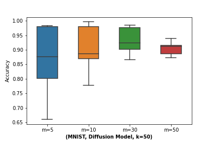
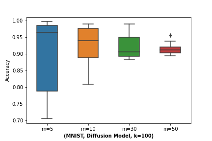
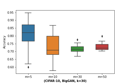
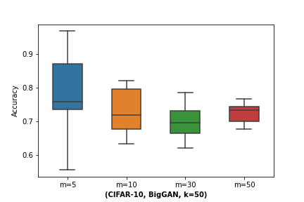
B-A Identical Class Test on Other Generative Models
We have presented Indetical Class Test (C1) on -VAE and MNIST [34], CIFAR-10 [35] in Sec V-A in our main context. Since GMValuator is model-agnostic, we further validate our method of C1 on other generative models.
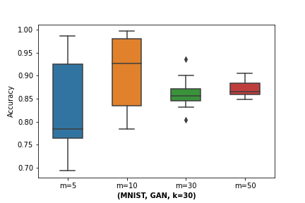
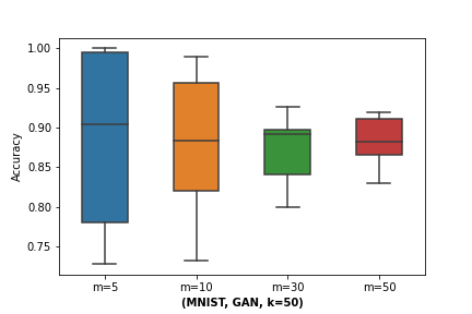
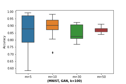
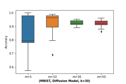
Here, we conduct the experiments using a GAN and a Diffusion Model on MNIST. The architectural details of the used generative models are described in Sec E-B in Appendix. We also conduct experiment on BigGAN [25] and Class-free Guidance Diffusion [32] with CIFAR-10. We used the same number of generated samples as the experiments presented in Sec V.
Following the similar settings in Sec. V-A (C1), we examine the class(es) of is top contributors for a given generated data in the training data. We calculate the number of training samples, denoted as , from the top contributors that have the same class as the generated data. The identical calss ratio, denoted as , is calculated as . We report the average value of across the generated datasets for different choices of in Table VI. GMValuator (DreamSim) has the highest ratio of contributors that belong to the same class as the generated sample among most of the models evaluated on MNIST and CIFAR-10 datasets for different values of . And the ratio improves as the value of decreases, which is consistent to the top assumption and validates our method.
B-B Identical Attributes Test on Other Datasets
To further validate GMValuator, we also conducted experiments on high-resolution datasets: AFHQ [37] and FFHQ [38], following the same settings in Sec V-B. The results are shown in Figure 6, which demonstrates the effectiveness of our methods in C2. The results show that the top contributors have the similar attributes with the generated sample such as the fur color of cats or dogs in AFHQ. For the experiment conducted on FFHQ, human faces attributes of the most significant contributors are also similar to the attributes in generated images.
Appendix C Different Generated Data Sizes
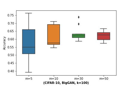
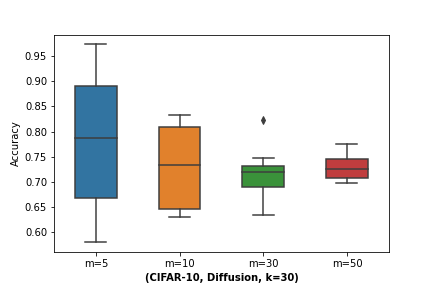
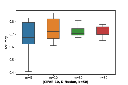
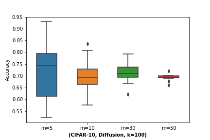
Since our value function (Eq. (3)) for training data is computed by averaging over generated samples, it is expected that the sensitivity of is connected to the size of the investigated generated sample. To explore the influence of generated data size on the utilization of GMValuator, we perform sensitivity testing on MNIST, CIFAR10 using generative models GAN [21], and Diffusion models [39] as depicted below. The dataset, model and used are denoted under each subfigure of Figure 7. First, we generate a varying number of samples from the same class. Specifically, we consider four different sample sizes, denoted by , which are given by 1, 10, 30, 50. Next, we evaluate the GMValuator using parameter C1, and this evaluation is performed for each of the aforementioned values of . Subsequently, we conduct the experiment 10 times using GMValuator (No-Rerank), each time with different -sized generated data samples from the same class. The results are presented as the mean and standard deviation () for accuracy, taken over these 10 runs. The results shown in Figure 7 imply that varying does not yield notable differences in mean accuracy and increasing the number of generated samples leads to more stable and consistent results.
Appendix D Alternative Distance Metric
We suggest utilizing Learned Perceptual Image Patch Similarity (LPIPS) [28] or DreamSim [27] as the distance metric during the re-ranking phase. This enables understanding the perceptual dissimilarity between generated and real data points. These metrics are applied in the image embedding space derived from pretrained models. Alternatively, distance measurement can be based on pixel space, such as employing -distance. Notably, we find that distances calculated in the input pixel space yield comparable outcomes as shown in Table VI. This implies that our method GMValuator could be flexible to the difference choices of distance metrics and the selection can depends on data prior.
Appendix E Additional Experimental Details
E-A Datasets
We conduct the generation tasks in the experiments on benchmark datasets (i.e., MNIST [34] and CIFAR [35]), face recognition dataset (i.e., CelebA [36]), and high-resolution image dataset AFHQ [37] and FFHQ [38].
MNIST. The MNIST dataset consists of a collection of grayscale images of handwritten digits (0-9) with a resolution of 28x28 pixels. The dataset contains 60,000 training images and 10,000 testing images.
CIFAR-10. CIFAR-10 dataset consists of 60,000 color images in 10 different classes, with 6,000 images per class. The classes include objects such as airplanes, cars, birds, cats, deer, dogs, frogs, horses, ships, and trucks. Each image in the CIFAR-10 dataset has a resolution of 32x32 pixels.
CelebA. The CelebA dataset is a widely used face recognition and attribute analysis dataset, which contains a large collection of celebrity images with various facial attributes and annotations. The dataset consists of more than 200,000 celebrity images, with each image labeled with 40 binary attribute annotations such as gender, age, facial hair, and presence of eyeglasses.
AFHQ. The AFHQ dataset is a high-resolution image dataset that focuses on animal faces (e.g., dogs, cat), and it consists of high-resolution images with 512 512 pixels.
FFHQ. The FFHQ dataset is a high-resolution face dataset that contains high-quality images (1024x1024 pixels) of human faces.
E-B Architecture of Generative models
In our experiments, we leverage different generative models in the class of GAN, VAE and diffusion model. We utilize -VAE for both MNIST and CIFAR-10 datasets while a simple GAN is conducted on MNIST. BigGAN and -VAE are also conducted on CIFAR-10. We list the architecture details for these generative models in Table VII. StyleGAN is used for high-resolution dataset AFHQ and FFHQ. CelebA uses Diffusion-StyleGAN [33], for which we use the exact architecture in their open sourced code.
Appendix F Discussion on the Possible Applications
The application of data valuation within generative models offers a wide range of opportunities. A potential use case is to quantify privacy risks associated with generative model training using specific datasets, since the matching mechanism GMValuator can help re-identify the training samples given the generated data. By doing so, organizations and individuals will be able to audit the usage of their data more effectively and make informed decisions regarding its use.
Another promising application is material pricing and finding in content creation. For example, when training generative models for various purposes, such as content recommendation or personalized advertising, data evaluation can be used to measure the value of reference content.
In addition, GMValuator can play an important role in the development of ensuring the responsibility of using synthetic data in safe-sensitive fields, such as healthcare or finance. By assessing the value of the data used in generative model training, researchers can ensure that the generated data are robust and reliable.
Last but not least, the applications of GMValuator can promote the recognition of intellectual property rights. Determining the value of the intellectual property being generated by generative models is critical. By evaluating the data employed in training generative models, we can develop a more comprehensive understanding of copyright that may emerge from the generative models. In essence, such insights can help advance licensing agreements for the utilization of the generative model and its outputs.
| GAN for MNIST | |
| Generator | Discriminator |
| FC(100, 8192), BN(32), ReLU | Conv2D(1, 128, 4, 2, 1), BN(128), LeakyReLU |
| Conv2D(128, 64, 4, 2, 1), BN(64), ReLU | FC(8192, 1024), BN(1024), LeakyReLU |
| BigGAN | ||||
| Input | 28281 (MNIST) & 32323 (CIFAR-10). | |||
| Encoder |
|
|||
| Latents | 32 | |||
| Decoder |
|
|||
| -VAE | |
| Generator | Discriminator |
| RGB image | |
| Linear | ResBlock down |
| ResBlock up | Non-Local Block |
| ResBlock up | ResBlock down |
| ResBlock up | ResBlock down |
| ResBlock up | ResBlock down |
| Non-Local Block | ResBlock down |
| ResBlock up | ResBlock |
| BN, ReLU, Conv ch | ReLU, Global sum pooling |
| Tanh | Embed linear |