Effects of large-scale magnetic fields on the observed composition
of ultra high-energy cosmic rays

Abstract

Ultra high-energy (UHE) cosmic rays (CRs) from distant sources interact with intergalactic radiation fields, leading to their spallation and attenuation. They are also deflected in intergalactic magnetic fields (IGMFs), particularly those associated with Mpc-scale structures. These deflections extend the propagation times of CR particles, forming a magnetic horizon for each CR species. The cumulative cooling and interactions of a CR ensemble also modifies their spectral shape and composition observed on Earth. We construct a transport formulation to calculate the observed UHE CR spectral composition for 4 classes of source population. The effects on CR propagation brought about by IGMFs are modeled as scattering processes during transport, by centers associated with cosmic filaments. Our calculations demonstrate that IGMFs can have a marked effect on observed UHE CRs, and that source population models are degenerate with IGMF properties. Interpretation of observations, including the endorsement or rejection of any particular source classes, thus needs careful consideration of the structural properties and evolution of IGMFs. Future observations providing tighter constraints on IGMF properties will significantly improve confidence in assessing UHE CR sources and their intrinsic CR production properties.

I Introduction

Ultra high-energy (UHE) cosmic-rays (CRs) are believed to originate in violent astrophysical environments, e.g. blazar jets, strongly magnetized neutron stars and starburst galaxies [see e.g. 2]. Their detection on Earth is rare [1], with arrival rates of about $1\;\!{\rm km}^{-2}\;{\rm yr}^{-1}$ being typical for particles with energies $E=10^{19}~{}{\rm eV}$ [see e.g. 3, 4, 5]. UHE CRs interact with baryons and photons as they propagate through intergalactic space. CR nuclei are converted to lighter particles via processes such as photo-spallation and photo-pion production. These attenuate CR fluxes and limit the survival distance of individual CRs. In the present Universe, CR protons with energies of $\sim 10^{19}\;\!{\rm eV}$ would undergo a photo-attenuation interaction over a few tens of Mpc [see e.g. 7]. It has therefore been argued that extragalactic UHE CRs of energies above $\sim 10^{19}\;\!{\rm eV}$ detected on Earth may originate from discernible sources within a photo-pion horizon distance of a few tens of Mpc [see 8, 9]. This is a reference distance, above which the Universe becomes ‘optically thick’ to UHE CR photo-pion attenuation.

UHE CRs could originate from more distant source populations located beyond their photo-pion horizon [e.g. 10, 11]. Their residual ‘background’ contribution can be used to study possible source population distributions over redshift because the cumulative effect of photo-spallation as the CR ensemble propagates modifies its arrival composition on Earth. This is also dependent on the effective travel-distances of UHE CR protons and nuclei, which are altered when magnetic fields are present [e.g. 12, 13, 14, 15]. Magnetic fields permeate intergalactic space. They are highly non-uniform, and could have fractal structures if associated with turbulence [see e.g. 16]. UHE CRs in intergalactic space are therefore not free streaming, nor do they gyrate around an ordered large-scale magnetic field. They are deflected in a stochastic manner [see e.g. 17, 18, 12, 19] and may also undergo diffusion [20, 21, 22].

Previous studies [see 4] investigated UHE CR composition and spectra the presence of intergalactic magnetic fields (IGMFs). Ref. [23] invoked 4-dimensional simulations to investigate the composition and anisotropy of UHE CRs with IGMFs at different positions in a simulation box when considering CR injection of ⁵⁶Fe or ¹H. Ref. [24] extended this to use a more physically-motivated UHE CR source composition. Other studies considered the effect of a magnetic field structure similar to the Local Super-cluster on CRs observed on Earth, and assessed the energy dependence of CR flux suppression caused by photo-pion attenuation and magnetic horizons [21]. Although large scale inhomogeneities from structures such as cosmic filaments and voids were not explicitly considered, secondary particle production was recently added as a refinement [see 22].

In this paper, we assess the effect of IGMFs on the spectrum and composition of UHE CRs. We consider different CR source populations and magnetic field prescriptions. To our knowledge, this study is the first to model CR propagation in IGMFs with inhomogeneities over cosmological scales, while properly accounting for photo-pion (absorption) and photo-spallation processes. It is also the first to assess the effects of an inhomogeneous IGMF on CR propagation and whether or not it can unambiguously be discerned in the observed CR spectrum and composition on Earth. The assumptions and methodology in our previous work [11] are adopted here, with, in addition, the treatment of the effects brought about by IGMFs.

We arrange this paper as follows. Section II.1 introduces CR source population models, compositions and their spectra. Section II.2 presents our treatment of UHE CR interactions. We introduce our demonstrative magnetic field prescriptions in Section II.3. Section III shows our results and discusses their implications. A summary of our findings is provided in Section IV.

Parameter	Definition	Value
$n_{c}$	Comoving number density of scattering centers	$10^{-2}$ Mpc-3
$\sigma_{c}$	Effective scattering center cross sectional size	3 Mpc2
$r_{c}$	Characteristic diameter of scattering center	2 Mpc
$\lambda_{c}$	Magnetic field coherence length within the scattering structure	0.3 Mpc

Table 1: Fiducial parameter choices for our illustrative magnetic field prescription. This considers cosmic filaments as the dominant scattering agent. Filament properties are based on the prescription introduced by [12]. The magnetic field strength evolves over redshift (see Fig. 1).

II Cosmic ray sources, propagation and interactions

II.1 Source population models

We consider four UHE CR source population models, specified over a redshift range from $z_{\rm min}=0$ to $z_{\rm max}=3$. For each model, the source number density in redshift space, composition and injected CR energy spectra follows the same paramatrization as in [11]. We summarize the source population models and the corresponding paramatrizations as follows. The first is the SFR model. It follows the redshift evolution of cosmic star formation (see also [25]) and takes the form:

$${\psi_{\rm SFR}(z)=\psi_{\rm SFR}^{0}\;\!\frac{(1+z)^{k_{1}}}{1+[(1+z)/k_{2}]^{k_{3}}}\ ,}$$ (1)

where $k_{1}=2.7$, $k_{2}=2.9$, $k_{3}=5.6$ and $\psi_{\rm SFR}^{0}=0.054$. The second is the GRB model. This is an adjustment of the SFR model and represents a possible redshift distribution of gamma-ray bursts. Its construction is based on Swift observations that indicate a similar redshift distribution to cosmic star-formation, but with an enhancement at earlier epochs. For the GRB model, we consider a redshift distribution,

$${\psi_{\rm GRB}(z)=\psi_{\rm GRB}^{0}\;\!(1+z)^{k_{4}}\;\!\psi_{\rm SFR}(z)\ ,}$$ (2)

where $k_{4}=1.4$ and $\psi_{\rm GRB}^{0}=0.013$, following [26]. The third is the AGN model. We adopt an AGN population evolution parametrization, given by [27]:

$${\psi_{\rm AGN}(z)=\psi_{\rm AGN}^{0}\left\{\begin{array}[]{ll}(1+z)^{k_{5}}&(z<z_{1})\\ {z_{2}}^{k_{5}}&(z_{1}\leq z<z_{2})\\ {z_{2}}^{k_{5}}\cdot{z_{2}}^{z_{2}-z}&(z\geq z_{2})\end{array}\right.\ ,}$$ (3)

where $k_{5}=5.0$, $z_{1}=1.7$, $z_{2}=2.7$ and $\psi_{\rm AGN}^{0}=0.0041$. The fourth is the PLW model. It parameterizes the source population by a power-law distribution in redshift space, as:

$${\psi_{\rm PLW}(z)=\psi_{\rm PLW}^{0}\;\!(1+z)^{k_{\rm PLW}}\ ,}$$ (4)

with $k_{\rm PLW}=-1.6$ and $\psi_{\rm PLW}^{0}=1.1$. This model is not specifically based on observations or a survey. It serves instead as a generic basis for comparison with similar PLW-type models that are employed in some other studies [e.g. 28, 29].

Here, the same spectral forms as in [11] are adopted for UHE CRs (see their Table 1). The overall injection luminosity in each model is normalized by gauging against Pierre Auger Observatory (PAO) data without detailed fitting. The energy range of the spectra is between $\epsilon_{\mathrm{min}}m_{\rm e}c^{2}=3.98\times 10^{18}\;\!{\rm eV}$ and $\epsilon_{\mathrm{max}}m_{\rm e}c^{2}=3.16\times 10^{20}\;\!{\rm eV}$. This is chosen to cover the CR flux contributed mostly by extragalactic particles [30, 31], and extends up to the most energetic UHE CRs expected to be detected on Earth [32].

In each source class the full range of injected nuclei are represented by the abundances of ²⁸Si, ¹⁴N, ⁴He, and ¹H. The injected composition fractions follow the fitted values of the species given in [29]. Variation of these fixed parameters would lead to a larger number of calculations and introduce more uncertainty, but would not improve the accuracy of our results. In our calculations, the production of all secondary nuclei species of mass number $A<28$ are properly accounted for. This safeguards the correct determination of photo-spallation interactions and their secondary products along particle propagations (see Section II.2).

II.2 Propagation and interactions of ultra high-energy cosmic ray nuclei

UHE CR nuclei are subject to hadronic interactions and energy losses as they propagate through intergalactic space. A CR particle may lose only a small fraction of its energy in a single interaction event, or it may lose energy continuously (such processes include photo-pair production, Compton scattering, radiative losses, or adiabatic energy losses in an expanding volume or space-time). We model these as effective “cooling” processes. In some situations, a CR particle loses substantial energy in a single interaction (e.g. photo-pion production) or can be split (photo-spallation). We treat these as absorption processes. In the case of photo-spallation events, we self-consistently account for the production of descendant nuclei using appropriate injection terms.

In the absence of IGMFs, the propagation of UHE CRs across intergalactic space is practically ballistic streaming at $c$, the speed of light. The corresponding CR transport equation is

$$\frac{\partial\;\!{n_{A}}}{\partial z} =\frac{{\rm d}s}{c\;\!{\rm d}z}\left[\frac{\partial}{\partial\epsilon_{A}}\left(b_{A}n_{A}\right)+{Q}_{A}-\Lambda_{A}n_{A}\right]\ ,$$ (5)

when adopting a quasi-steady condition [11]. Here, the particle species is specified by mass number $A$. $n_{A}(\epsilon_{A},z)$ is the comoving spectral density of UHE CRs with mass number $A$ and dimensionless energy $\epsilon_{A}$, $b_{A}$ is the total energy loss rate experienced by those CRs due to cooling processes and $\Lambda_{A}={\Lambda^{\rm sp}}_{\!A}+{\Lambda^{A\pi}}_{\!A}$ is the total absorption rate accounting for photo-spallation (${\Lambda^{\rm sp}}_{\!A}$) and photo-pion production (${\Lambda^{A\pi}}_{\!A}$). $Q_{A}=Q_{A}^{\rm a}+Q_{A}^{\rm sp}$ is the injection rate of UHE CRs. This is the sum of photo-spallation products (secondary nuclei) $Q_{A}^{\rm sp}$ and fresh primary particle injection $Q_{A}^{\rm a}$ by the source population. In a Friedmann-Lemaître-Robertson-Walker (FLRW) universe,

$$\frac{{\rm d}s}{{c\;\!\rm d}z} =\frac{\mathcal{E}(z)}{H_{0}\;\!(1+z)}\ ,$$ (6)

where $H_{0}$ is the present value of the Hubble parameter. This takes a value of $100\;\!h\;\!{\rm km}\;\!{\rm s}^{-1}{\rm Mpc}^{-1}$, $h=0.673\pm 0.006$ [33], and

$$\mathcal{E}(z)=\left[\Omega_{\rm r,0}(1+z)^{4}+\Omega_{\rm m,0}(1+z)^{3}+\Omega_{\rm\Lambda,0}\right]^{-1/2}$$ (7)

[see 34], with $\Omega_{\rm m,0}=0.315\pm 0.007$, $\Omega_{\rm r,0}\approx 0$ and $\Omega_{\rm\Lambda,0}=0.685\pm 0.007$. These are the normalized density parameters for matter, radiation and dark energy, respectively [33].

If accommodating IGMFs into our formulation, CR transport is modified across intergalactic space. IGMFs have certain structures associated with density distributions, which may be in the form of galaxies, galaxy groups/clusters and cosmic filaments. They could also be turbulent in nature. A comprehensive treatment of UHE CR propagation, properly accounting for the effects of magnetic fields convolved with those of density structures of objects across the mass hierarchy in the Universe is non-trivial. This subject has been addressed in previous studies, which provide insights into transitions to diffusive propagation in detailed configurations of turbulence [e.g. 35, 36, 37], including the effects of magnetic intermittency [38], and by invoking increasingly detailed simulations [e.g. 23, 39].

We consider that CR transport in localized regions of enhanced magnetic fields may be treated as a series of discrete scattering events. Hereafter, we refer to scattering events that lead to the deflection of CR particles as ‘deflections’. Magnetized regions are associated with particular astrophysical environments which act as scattering centers (e.g. galaxy clusters or cosmic filaments; see [40, 12]). This heuristic treatment captures the main essence of UHE CR transport in intergalactic space in the presence of IGMFs when the accumulated deflection angle of the CRs is small. It is justified, as the linear sizes of the scattering structures (e.g. cosmic filaments, which would be a few Mpc [e.g. 41, 42]) are much smaller than either the spacing between structures ($\sim$ 100 Mpc [e.g. 43]), or the photo-pion horizon scale of the CR particles.

Our formulation is essentially 1-dimensional (1D) and the effects of deflections are captured in an effective difference in path length. The additional path length of weakly scattered particles (with a deflection angle much smaller than $\pi/2$) compared to free streaming CR propagation is expressed as

$$\delta s^{\prime} =N_{c}\;\!{\delta t_{c}^{\prime}}\;\!c\ .$$ (8)

Here, $N_{c}$ is the number of scattering events a CR undergoes along a path. In an interval $\delta s$, this is given by $N_{c}=\delta s/d_{c}$, where $d_{c}=(n_{c}\;\!\sigma_{c})^{-1}$ is the mean free path of a CR to an interaction with a scattering center. $n_{c}$ and $\sigma_{c}$ are the comoving number density and physical effective cross sectional size of the scattering centers, respectively. The extra propagation time $\delta t_{c}^{\prime}$, introduced when a CR is deflected into an longer, non-rectilinear path by a scattering event, plus the delay time it experiences when crossing each scattering center, can be expressed as

$$\delta t_{c}^{\prime} \simeq\frac{d_{\rm c}\;\!\delta{\theta_{c}}^{2}}{8c}+\frac{\bar{r}_{c}\;\!\delta{\theta_{c}}^{2}}{6\;\!c}\$$ (9)

[44, 12]. The first term above accounts for the time delay associated with the non-rectilinear trajectory arising from the scattering event. The second term accounts for the time delay with respect to straight line when a CR crosses a magnetized scattering structure. $\bar{r}_{c}$ is the characteristic path length through a scattering center. This is related to the physical size of the scattering center $r_{c}$ by $\bar{r}_{c}=(\pi/2)^{2}\;\!r_{c}$ (for a filamentary morphology [12]). The deflection angle $\delta\theta_{c}$, is given by

$$\delta{\theta_{c}}^{2} \simeq\left(1+\frac{2\;\!{r_{L}}^{2}}{\bar{r}_{c}\lambda_{c}}\right)^{-1}\ ,$$ (10)

where $\lambda_{c}$ is the coherence length of the magnetic field of the scattering structure. $r_{L}$ is introduced as the charged particle’s gyro-radius, which depends on the CR charge $Z_{A}$, energy $\epsilon_{A}$ and the magnetic field strength of the scattering center:

$$r_{L} \approx 1.1\;\!\left(\frac{\epsilon_{A}}{2\times 10^{12}}\right)\left(\frac{B}{1\;\!{\rm nG}}\right)^{-1}\left(\frac{Z_{A}}{1}\right)^{-1}{\rm Mpc}\ .$$ (11)

Equation 10 is adopted for the transition from $r_{L}\ll\sqrt{r_{c}\lambda_{c}}$ (when the particle exits a scattering center with a small deflection angle after undergoing a single scattering event) to $r_{L}\gg\sqrt{r_{c}\lambda_{c}}$ (where the particle diffuses within the scattering structure, and exits roughly at the same location it entered; see [12]). The overall path length taking account of the effects of deflections is then given by $\delta s^{\prime}=\delta s+c\delta t_{c}^{\prime}$.

For the propagation of some CRs, the accumulated deflection angle can become large ($>\pi/2$). The CR transport in this situation is instead modeled using a strong deflection prescription, where the additional path lengths experienced by CRs are given by $\delta s^{\prime\prime}=\delta s^{\prime}(1+\Delta s^{\prime}/\ell_{\rm scatt})$. Here, $\Delta s^{\prime}$ is the integrated path length, and $\ell_{\rm scatt}=(n_{c}\;\!\sigma_{c}\;\!{\delta\theta_{c}}^{2})^{-1}$ is the scattering distance over which the CRs experience a strong deflection. With the additional path lengths properly incorporated in the calculations of photo-pion interactions and photo-spallation, we obtain a revised relation for the CR travel time and propagation distance.

With equation 8, we construct a scaling factor for the fractional path length extension experienced by the propagating CRs due to deflections:

$$\Psi_{A}=\frac{\delta s^{\prime\prime}}{\delta s}=\frac{\delta s^{\prime}(1+\Delta s^{\prime}/\ell_{\rm scatt})}{\delta s}$$ (12)

Applying this to the transport equation (equation 5), we obtain

$$\frac{\partial\;\!{n_{A}}}{\partial z}=\frac{{\rm d}s}{c\;\!{\rm d}z}\bigg{(}\Psi_{A}\bigg{[}\frac{\partial}{\partial\epsilon_{A}}(b_{A}n_{A} )+\phi_{\rm A}^{B}\;\!Q_{A}^{\rm sp}-\Lambda_{A}n_{A}\bigg{]}+{Q}_{A}^{\rm a}\bigg{)}\ .$$ (13)

Note that this omits an explicit treatment of diffusion, with its effects considered only in the path length scaling term $\Psi_{\rm A}$. This is justified in the computation of the total diffuse average fluxes when the overall CR deflection angles accumulated over their total path length are sufficiently small, or when the separation between sources is shorter than both the diffusion length and the CR energy loss distance [45, 12].

The magnetic scaling term is applied to all propagation, interaction and cooling terms. The primary source term ${Q}_{A}^{\rm a}$ is independent of the magnetic fields. It is distinct from another source term $Q_{A}^{\rm sp}$. This depends on the photo-spallation rate of parent CRs of higher nucleon number. The propagation of the parent nuclei are modified by a scaling factor appropriate for their species, $\Psi_{\rm B}$. This is related to $\Psi_{\rm A}$ by the ratio of the squared deflection angles of the parent and secondary CRs, denoted $\phi_{A}^{B}$.

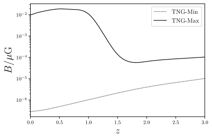
Figure 1: Evolution of magnetic field strength over redshift $z$ derived from the IllustrisTNG 100-3 simulations [46, 47]. An interpolation routine is used for cosmological epochs between simulation redshift slices. The TNG-Max prescription is the median magnetic field strength in structures with a baryon over-density with $\log_{10}(\rho/\langle\rho_{b}\rangle)=2$; TNG-Min is for $\log_{10}(\rho/\langle\rho_{b}\rangle)=0.7$. This covers the range of densities appropriate for cosmic filaments [46].

II.3 Intergalactic magnetic field prescriptions

The fiducial magnetic field configuration is adapted from [12]. The effective size, number density and magnetic-field coherence length of the scattering centers are chosen such that they are appropriate for cosmic filaments (Table I). The evolution of the filaments is not considered explicitly, as their size does not change substantially over in the redshifts considered in this study [42]. The magnetic fields in the filaments, however, evolve, as shown in numerical simulations [see e.g. 48]. We use the results from IllustrisTNG 100-3 simulations [46, 47, 49, 50, 51, 52]) to construct two redshift-dependent IGMF-strength prescriptions (presented in Fig. 1).

The effects of IGMFs on the propagation of UHE CRs with energies between $10^{17}$ eV and $10^{21}$ eV by deflections in cosmic filaments can be comparable to magnetized structures on galactic scales, in particular, fossil radio galaxies and galactic winds [12]. In our calculations, these substructures are incorporated implicitly in the effective scattering of the filaments through a maximum and minimum limit, which brackets the extent of their effects.

III Results and discussion

III.1 UHE CR spectrum and composition

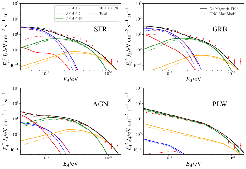
Figure 2: UHE CR flux spectra of the four source population models (SFR, GRB, AGN and PLW) at $z=0$. Solid lines represent scenarios with no IGMFs. Dotted lines represent the scenarios with IGMFs, whose strength evolves according to the TNG-Max prescription (see Section II.3). Magnetic horizon effects reduce the overall primary particle flux in the TNG-Max prescription. This is more pronounced in source distributions with heavier compositions, which have shorter magnetic horizon distances. If source distributions are weighted towards higher redshifts and the injection composition is relatively low-mass, secondary production can increase the particle flux at low energies (e.g. as in the SFR and GRB cases). The corresponding results for the TNG-Min prescription are not shown. These are very similar to scenarios without IGMFs. Data obtained by PAO [53] (red dots with error bars) are shown for comparison. Note that the $1\leq A\leq 2$ line for the PLW case without magnetic fields falls below the range of the axes. In all models, a further secondary $A=1$ particle component emerges slightly below 10²⁰ eV (also below the axes range). These originate from photo-spallation interactions of very energetic heavy CRs with EBL photons. Their contribution is negligible.

The UHE CR spectrum at $z_{\rm min}=0$ for each source class is obtained by integrating the modified transport equation (equation 13) numerically over a discretized grid in redshift. The effect of the evolving magnetic field is accounted for by calculating the average value of the scaling factor $\Psi_{A}$ between subsequent grid points. The extra path lengths accounting for CR deflections extends the propagation times of the particles. In some cases, this may exceed the Hubble time. Such particles will not reach us, forming a magnetic horizon [54, 55]. Their contribution is excluded in the calculations by setting an upper limit in the integration of $z_{\rm max}=\min\left\{z_{\rm H},3\right\}$, where $z_{\rm H}$ is the redshift at which the total propagation time of a CR undergoing deflections would equal the age of the Universe. This effect changes the total CR arrival flux of each of the species. The all-particle spectrum and four broadband composition spectra are shown in Fig. 2. For scenarios with no IGMFs, our results are identical to those obtained for streaming CRs. If weak IGMFs are present, e.g. TNG-Min (not shown), their effects on CR propagation are insufficient to give results which are noticeably different to scenarios without IGMFs. These results are generally consistent with PAO data [53].

Effects caused by deflections are important in the TNG-Max prescription. The results are more difficult to reconcile with the PAO observations [53] (especially for scenarios invoking SFR or GRB source classes). In this situation, strong deflections can become important for some CRs (see Fig. 3). These CRs would propagate via diffusion. The relatively small separation between the sources in our model is less than the CR diffusion length and energy loss distance. Under these conditions, the diffuse average flux spectrum is well approximated by the streaming treatment with deflections adopted here [45].

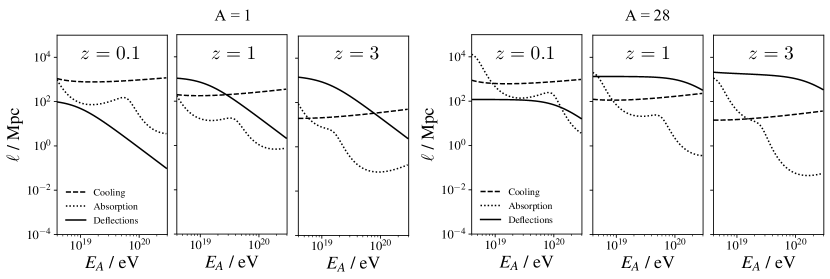
Figure 3: UHE CR cooling (dashed lines), absorption/spallation (dotted lines) distances, and cumulative extra path lengths introduced by deflections (solid lines) in CR propagation scenarios in IGMFs described by the TNG-Max model, from $z=0$ up to $z=0.1$, 1 and 3, as stated. The cumulative extra path lengths only increase significantly up to $z=1$, reflecting the epoch where the evolving IGMF is strongest (see Fig. 1). For $A=1$, absorption is due to photo-pion production. Photo-spallation is the dominant absorption process for heavier nuclei.

The effects of IGMFs on the CR spectrum and composition are shown in Fig. 2. They are manifestations of the competition between cooling and absorption, secondary nuclei production and magnetic horizon effects. Qualitatively, we may discern two regimes by CR energy. At energies above $\sim 3\times 10^{19}$ eV, deflections introduce an extra CR path length of hundreds of Mpc. This is longer than photo-spallation lengths, particularly for heavy CR nuclei (see Fig. 3). Cooling lengths at these energies are much longer than attenuation lengths. The high energy spectrum of particles is therefore dominated by the injection of primary CRs, and the effects of cooling are obscured by attenuation.

While magnetic fields do not have strong effects on the horizon for CRs with extremely high energies, the situation is different for CRs with energies below $\sim 3\times 10^{19}~{}{\rm eV}$ where the extended path lengths range between tens to hundreds of Mpc. This is shorter than the photo-pion and photo-spallation length scales at $z<1$ for low mass nucleons, but becomes comparable at higher masses (see Fig. 3). As photo-spallation (for $A>1$) at these energies always dominates over photo-pion absorption, secondary CRs with low mass ($1\leq A\leq 2$) accumulate. At high redshifts, this accumulation is partially countered by photo-pion attenuation and magnetic horizons in the extended path lengths and does not greatly affect the spectrum observed at $z=0$. At lower redshifts, the longer attenuation path lengths mean that the accumulation of secondaries in the presence of IGMFs is more apparent, especially when the injected composition of CRs is of relatively low-mass. As photo-pair lengths are shorter than the extended path lengths and also comparable to attenuation length scales, noticeable cooling effects on the low-mass components of the particle spectrum emerge (in particular, for $A\leq 6$ in the SFR and GRB models). The combination of all these effects in the extended propagation paths experienced by CRs in the presence of IGMFs distort the average mass composition $\langle\ln A\rangle$ at $z=0$, and generally boost the relative abundance of lower-mass nuclei at lower energies (see Fig. 4).

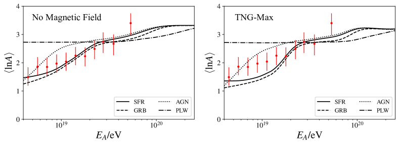
Figure 4: Average UHE CR mass composition $\langle\ln A\rangle$ for the four source classes. The left panel shows scenarios where deflections in the IGMFs are not considered. The right panel shows the composition when adopting the TNG-Max prescription. Results obtained with the TNG-Min prescription are indistinguishable from scenarios neglecting IGMFs. The data points shown in red were obtained from PAO [56, 57] (using Sibyll 2.3c [58, 59]).

III.2 Scattering centers and CR source population models

When comparing the PAO spectral and composition data in Figs. 2 and 4, scenarios predicting a strong secondary CR component would appear to be less favorable. In the presence of filament magnetic fields of 10s of nG below $z\sim 1$, source distributions weighted towards higher redshifts (e.g. AGN populations as CR sources) are preferred. However, source populations (initial conditions) and magnetic field prescriptions (a component in the transport process) are degenerate when matching the results of calculations with observations.

In this work, we consider a single type of scattering center – cosmic filaments. Fig. 5 show also other scattering center candidates for comparison. Limits bounding each region are set by the approximate range of characteristic sizes, their spatial abundance in the Universe, any knowledge of the magnetic fields inherent to each environment, and observational constraints (obtained from [16, 61, 62]; see Appendix A). This is presented in terms of two quantities, $X=n_{c}\;\!r_{c}^{2}\;\!\sigma_{c}$ ($\propto n_{c}\;\!r_{c}^{4}$) and $Y=B_{c}^{2}\;\!\lambda_{c}$, for which the product is proportional to the magnetic scaling factor $\Psi_{A}$ (see equation 12). The top-right of Fig. 5 represents conditions where the deflection potential is stronger.

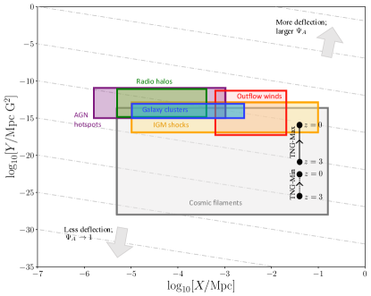
Figure 5: Comparison of the ability of scattering center types to deflect UHE CRs. Here, $X=n_{c}\;\!{r_{c}}^{2}\;\!\sigma_{c}$ ($\propto n_{c}\;\!{r_{c}}^{4}$) and $Y={B_{c}}^{2}\;\!\lambda_{c}$. Regions towards the top right yield stronger deflections. The evolutionary progression of the TNG-Min and TNG-Max prescriptions (see section III.1) are marked by black arrows. Contours of equal deflection are represented by gray dot-dashed lines. Candidate classes of scattering centers are represented by rectangular boxes, where boundaries are set by theoretical or observational constraints (see Appendix A).

Figs. 2 and 4 show that the effects of IGMFs become substantial at low redshifts for the TNG-Max prescription, and are inconsequential for the TNG-Min prescription. The parameter space where the effects of deflections are important lies above a contour through the mid-point of the TNG-Max line in Fig. 5. This passes through the allowed regions of all scattering centers considered. Constraints obtained by current observations or theoretical studies are insufficient for distinguishing the merits of the different classes of scattering centers. This must be properly addressed when endorsing any UHE CR source class. For example, most source populations are acceptable if IGMFs are ignored, but none are acceptable if the TNG-Max prescription is used to derive the IGMF strength and its evolution. Nonetheless, Fig. 5 provides useful insights for identifying possible scattering centers, and for modeling their effects on CR transport. With up-coming instruments (e.g. the Square Kilometer Array, SKA) dedicated to study the magnetic properties of the hierarchy of structures in the Universe, more advanced modeling of IGMFs will be possible down to galactic scales. With these new insights, transport calculations with a proper astrophysical set up and robust parameter choices will allow us to confidently resolve the origins of UHE CRs.

IV Summary

We investigate the effects of IGMFs on the propagation of UHE CRs and on the CR spectrum and composition observed at $z=0$. We solve the particle transport equation accounting for the deflections of CRs by IGMFs, and the cumulative effects of absorption, spallation and interactions with intergalactic radiation fields. Piece-wise deflections of CR particles by IGMFs are modeled as stochastic scattering by centers associated with cosmic filaments. The properties of the filaments and the evolution of their magnetic field strengths are derived from cosmological simulations. Our calculations have shown that IGMFs can have a marked effect on the observed properties of UHE CRs detected on Earth, when the IGMF strength reaches 10s of nG for cosmic filaments by $z\mathrel{\raise 1.29167pt\hbox{$<$\kern-7.5pt\lower 4.30554pt\hbox{$\sim$}}}1$. We find the source population models and IGMFs are degenerate. This degeneracy must be properly resolved before endorsing or disfavoring different UHE CR source classes (including those not considered in this work) to determine the origin of components in broad composition spectra of UHE CRs observed on Earth. Refinement of the results obtained in this work can be achieved by improving the modeling of the IGMFs in cosmic filaments and their substructures. Observations by near-future facilities, in particular, the SKA, will advance our knowledge of the hierarchical properties of magnetic fields from scales of galaxies and clusters to filaments and voids, thus providing more robust inputs for modeling the scattering of UHE CRs by IGMFs in transport calculations.

Acknowledgments: We thank the anonymous referees for their constructive comments. ERO is an overseas researcher under the Postdoctoral Fellowship of the Japan Society for the Promotion of Science (JSPS), supported by JSPS KAKENHI Grant Number JP22F22327, and also acknowledges support from the Center for Informatics and Computation in Astronomy (CICA) at National Tsing Hua University (NTHU) through a grant from the Ministry of Education (MoE) of Taiwan (ROC), where part of this study was conducted. QH is supported by a UCL Overseas Research Scholarship and a UK Science and Technology Facilities Council (STFC) Research Studentship. QH and KW acknowledge support from the UCL Cosmo-particle Initiative. This study is supported in part by a UK STFC Consolidated Grant awarded to UCL-MSSL. This work made use of high-performance computing facilities operated by CICA at NTHU. This equipment was funded by the MoE and the National Science and Technology Council of Taiwan (ROC). This work made use of IllustrisTNG simulations, which were undertaken with compute time awarded by the Gauss Centre for Supercomputing (GCS) under GCS Large-Scale Projects GCS-ILLU and GCS-DWAR on the GCS share of the supercomputer Hazel Hen at the High Performance Computing Center Stuttgart (HLRS), as well as on the machines of the Max Planck Computing and Data Facility (MPCDF) in Garching, Germany. This work made use of the NASA ADS database.

Appendix A Scattering centers

Type Parameter value range $n_{c}$/Mpc^-3 $r_{c}$/Mpc $\lambda_{c}$/Mpc $B_{c}$/$\mu$G Cosmic filaments $(0.3-1)\times 10^{-2}$ See note^(a) $0.2-2$ Ref. [63] See note^(b) $10^{-5.5}-10^{-1}$ Ref. [46] Galaxy clusters $10^{-5}$ Ref. [12, 64] $1-4$ Ref. [65] 0.1 See note^(c) $10^{-1}-10^{0}$ Ref. [66, 67] Galactic outflow winds $(1-5)\times 10^{-2}$ Ref. [12, 68] $0.5-0.8$ Ref. [12] 0.05 Ref. [12] $10^{-2}-10^{1}$ Ref. [69, 70] Radio halos $5\times 10^{-6}$ Ref. [71]^(d) $1-3$ Ref. [72, 73] 0.1 See note^(c) $10^{-1}-10^{1}$ Ref. [12, 74] IGM accretion shocks around clusters $10^{-5}$ See note^(e) $1-10$ Ref. [75] 0.1 See note^(c) $10^{-2}-10^{0}$ Ref. [76] AGN terminating bow shocks (hot spots) $10^{-3}$ Ref. [77]^(f) $0.2-1$ Ref. [74, 78] 0.1 See note^(c) $10^{-1}-10^{1}$ Ref. [79, 74]

Table 2: Scattering centers parameters, as in Fig. 5. Notes: (a) Values estimated from the sizes of voids separating filaments, combined with the indicated $r_{c}$ range (to estimate a filament cross section). (b) This value is not specified. Constraints of $\lambda_{c}$ are derived from those in [16, 61, 62] based on adopted $B_{c}$ values, where $\lambda_{c}$ has an upper limit of $r_{c}$. (c) Default value is used for IGMFs (see, e.g. [80]). (d) Based on [71], we assume that 50% of clusters host radio halos. This fraction depends on cluster mass and merging history. (e) We assume this to be the same as for galaxy clusters, where accretion shocks are often present. (f) Estimated from X-ray selected AGN, many of which tend to have hot spots.

The ranges of parameter values adopted for each type of scattering center shown in Fig. 5 are summarized in Table II.

References

- [1] M. Kachelrieß and D. V. Semikoz, Prog. Part. Nucl. Phys. 109, 103710 (2019), 1904.08160.
- [2] L. A. Anchordoqui, Phys. Rep. 801, 1 (2019), 1807.09645.
- [3] A. A. Watson, Rep. Prog. Phys. 77, 036901 (2014), 1310.0325.
- [4] R. Alves Batista et al., Frontiers in Astronomy and Space Sciences 6, 23 (2019), 1903.06714.
- [5] A. Aab et al., Phys. Rev. D102, 062005 (2020), 2008.06486.
- [6] R. Aloisio, V. Berezinsky, and S. Grigorieva, Astroparticle Physics 41, 94 (2013), 1006.2484.
- [7] C. D. Dermer and G. Menon, High Energy Radiation from Black Holes: Gamma Rays, Cosmic Rays, and Neutrinos (Princeton University Press, 2009).
- [8] K. Greisen, Phys. Rev. Lett. 16, 748 (1966).
- [9] G. T. Zatsepin and V. A. Kuz’min, Soviet Journal of Experimental and Theoretical Physics Letters 4, 78 (1966).
- [10] V. S. Berezinskii and S. I. Grigor’eva, Astron. Astrophys. 199, 1 (1988).
- [11] E. R. Owen, Q. Han, K. Wu, Y. X. J. Yap, and P. Surajbali, Astrophys. J. 922, 32 (2021), 2107.12607.
- [12] K. Kotera and M. Lemoine, Phys. Rev. D77, 123003 (2008), 0801.1450.
- [13] A. M. Taylor and F. A. Aharonian, Phys. Rev. D79, 083010 (2009), 0811.0396.
- [14] F. Capel and D. J. Mortlock, Mon. Not. R. Astron. Soc. 484, 2324 (2019), 1811.06464.
- [15] A. van Vliet, A. Palladino, A. Taylor, and W. Winter, Mon. Not. R. Astron. Soc. 510, 1289 (2022), 2104.05732.
- [16] R. Durrer and A. Neronov, Astron. Astrophys. Rev. 21, 62 (2013), 1303.7121.
- [17] J. Giacalone and J. R. Jokipii, Astrophys. J. 520, 204 (1999).
- [18] H. Yan and A. Lazarian, Astrophys. J. 673, 942 (2008), 0710.2617.
- [19] S. Xu and H. Yan, Astrophys. J. 779, 140 (2013), 1307.1346.
- [20] K. Kotera and M. Lemoine, Phys. Rev. D77, 023005 (2008), 0706.1891.
- [21] S. Mollerach and E. Roulet, J. Cosmol. Astropart. Phys. 2013, 013 (2013), 1305.6519.
- [22] J. M. González, S. Mollerach, and E. Roulet, Phys. Rev. D104, 063005 (2021), 2105.08138.
- [23] R. Alves Batista, M.-S. Shin, J. Devriendt, D. Semikoz, and G. Sigl, Phys. Rev. D96, 023010 (2017), 1704.05869.
- [24] D. Wittkowski, Proc. Sci. ICRC2017, 563 (2017).
- [25] M. S. Muzio, M. Unger, and G. R. Farrar, Phys. Rev. D100, 103008 (2019), 1906.06233.
- [26] X.-Y. Wang, R.-Y. Liu, and F. Aharonian, Astrophys. J. 736, 112 (2011), 1103.3574.
- [27] G. Hasinger, T. Miyaji, and M. Schmidt, Astron. Astrophys. 441, 417 (2005), astro-ph/0506118.
- [28] A. M. Taylor, M. Ahlers, and D. Hooper, Phys. Rev. D92, 063011 (2015), 1505.06090.
- [29] R. Alves Batista, R. M. de Almeida, B. Lago, and K. Kotera, J. Cosmol. Astropart. Phys. 2019, 002 (2019), 1806.10879.
- [30] G. Giacinti, M. Kachelrieß, D. V. Semikoz, and G. Sigl, J. Cosmol. Astropart. Phys. 2012, 031 (2012), 1112.5599.
- [31] R. Aloisio, V. Berezinsky, and P. Blasi, J. Cosmol. Astropart. Phys. 2014, 020 (2014), 1312.7459.
- [32] D. J. Bird et al., Astrophys. J. 441, 144 (1995), astro-ph/9410067.
- [33] Planck Collaboration et al., Astron. Astrophys. 641, A6 (2020), 1807.06209.
- [34] J. A. Peacock, Cosmological Physics (Cambridge University Press, 1999).
- [35] M. Ahlers, Phys. Rev. Lett. 112, 021101 (2014), 1310.5712.
- [36] R. Alves Batista and G. Sigl, J. Cosmol. Astropart. Phys. 2014, 031 (2014), 1407.6150.
- [37] A. D. Supanitsky, J. Cosmol. Astropart. Phys. 2021, 046 (2021), 2007.09063.
- [38] A. Shukurov, A. P. Snodin, A. Seta, P. J. Bushby, and T. S. Wood, Astrophys. J. Lett. 839, L16 (2017), 1702.06193.
- [39] A. Arámburo-García et al., Phys. Rev. D104, 083017 (2021), 2101.07207.
- [40] G. Medina-Tanco and T. A. Enßlin, Astroparticle Physics 16, 47 (2001), astro-ph/0011454.
- [41] A. G. Doroshkevich, D. L. Tucker, R. Fong, V. Turchaninov, and H. Lin, Mon. Not. R. Astron. Soc. 322, 369 (2001).
- [42] M. Cautun, R. van de Weygaert, B. J. T. Jones, and C. S. Frenk, Mon. Not. R. Astron. Soc. 441, 2923 (2014), 1401.7866.
- [43] N. I. Libeskind et al., Mon. Not. R. Astron. Soc. 473, 1195 (2018), 1705.03021.
- [44] C. Alcock and S. Hatchett, Astrophys. J. 222, 456 (1978).
- [45] R. Aloisio and V. Berezinsky, Astrophys. J. 612, 900 (2004), astro-ph/0403095.
- [46] F. Marinacci et al., Mon. Not. R. Astron. Soc. 480, 5113 (2018), 1707.03396.
- [47] D. Nelson et al., Computational Astrophysics and Cosmology 6, 2 (2019), 1812.05609.
- [48] F. Vazza, M. Brüggen, C. Gheller, and P. Wang, Mon. Not. R. Astron. Soc. 445, 3706 (2014), 1409.2640.
- [49] J. P. Naiman et al., Mon. Not. R. Astron. Soc. 477, 1206 (2018), 1707.03401.
- [50] D. Nelson et al., Mon. Not. R. Astron. Soc. 475, 624 (2018), 1707.03395.
- [51] V. Springel et al., Mon. Not. R. Astron. Soc. 475, 676 (2018), 1707.03397.
- [52] A. Pillepich et al., Mon. Not. R. Astron. Soc. 475, 648 (2018), 1707.03406.
- [53] V. Verzi, Proc. Sci. ICRC2019, 450 (2019).
- [54] M. Lemoine, Phys. Rev. D71, 083007 (2005), astro-ph/0411173.
- [55] V. Berezinsky and A. Z. Gazizov, Astrophys. J. 669, 684 (2007), astro-ph/0702102.
- [56] Pierre Auger Collaboration, J. Cosmol. Astropart. Phys. 2013, 026 (2013), 1301.6637.
- [57] A. Yushkov, Proc. Sci. ICRC2019, 482 (2019).
- [58] F. Riehn et al., Proc. Sci. ICRC2017, 301 (2017).
- [59] A. Fedynitch, F. Riehn, R. Engel, T. K. Gaisser, and T. Stanev, Phys. Rev. D100, 103018 (2019), 1806.04140.
- [60] E. Carretti et al., Mon. Not. R. Astron. Soc. 512, 945 (2022), 2202.04607.
- [61] Planck Collaboration et al., Astron. Astrophys. 594, A19 (2016), 1502.01594.
- [62] J. L. Han, Annu. Rev. Astron. Astrophys. 55, 111 (2017).
- [63] C. Gheller and F. Vazza, Mon. Not. R. Astron. Soc. 486, 981 (2019), 1903.08401.
- [64] T. D. Oswalt and W. C. Keel, Planets, Stars and Stellar Systems Vol. 6 (Springer, 2013).
- [65] S. M. Hansen et al., Astrophys. J. 633, 122 (2005), astro-ph/0410467.
- [66] M. Brüggen, M. Ruszkowski, A. Simionescu, M. Hoeft, and C. Dalla Vecchia, Astrophys. J. Lett. 631, L21 (2005), astro-ph/0508231.
- [67] V. Vacca et al., Galaxies 6, 142 (2018).
- [68] M. Bianconi et al., Mon. Not. R. Astron. Soc. 492, 4599 (2020), 2001.04478.
- [69] V. Heesen, R.-J. Dettmar, M. Krause, R. Beck, and Y. Stein, Mon. Not. R. Astron. Soc. 458, 332 (2016), 1602.04085.
- [70] R. Pakmor et al., Mon. Not. R. Astron. Soc. 498, 3125 (2020), 1911.11163.
- [71] V. Cuciti et al., Astron. Astrophys. 580, A97 (2015), 1506.03209.
- [72] C. Xie et al., Astron. Astrophys. 636, A3 (2020), 2001.04725.
- [73] D. N. Hoang et al., Astron. Astrophys. 656, A154 (2021), 2106.00679.
- [74] T. Stanev, High Energy Cosmic Rays (Springer, 2010).
- [75] K. Kotera and A. V. Olinto, Annu. Rev. Astron. Astrophys. 49, 119 (2011), 1101.4256.
- [76] R. J. van Weeren, H. J. A. Röttgering, M. Brüggen, and M. Hoeft, Science 330, 347 (2010), 1010.4306.
- [77] J. D. Silverman et al., Astrophys. J. 624, 630 (2005), astro-ph/0406330.
- [78] M. Orienti et al., Mon. Not. R. Astron. Soc. 419, 2338 (2012), 1109.4895.
- [79] M. W. Werner et al., Astrophys. J. 759, 86 (2012), 1209.0810.
- [80] D. Ryu, H. Kang, J. Cho, and S. Das, Science 320, 909 (2008), 0805.2466.