Transdimensional surface wave tomography of the near-surface: Application to DAS data

Abstract

Distributed Acoustic Sensing (DAS) is a novel technology that allows sampling of the seismic wavefield densely over a broad frequency band. This makes it an ideal tool for surface wave studies. In this study, we evaluate the potential of DAS to image the near-surface using synthetic data and active-source field DAS data recorded with straight fibers in Groningen, the Netherlands. First, we recover the laterally varying surface wave phase velocities (i.e., local dispersion curves) from the fundamental-mode surface waves. We utilize the Multi Offset Phase Analysis (MOPA) for the recovery of the laterally varying phase velocities. In this way, we take into account the lateral variability of the subsurface structures. Then, instead of inverting each local dispersion curve independently, we propose to use a novel 2D transdimensional surface wave tomography algorithm to image the subsurface. In this approach, we parameterize the model space using 2D Voronoi cells and invert all the local dispersion curves simultaneously to consider the lateral spatial correlation of the inversion result. Additionally, this approach reduces the solution nonuniqueness of the inversion problem. The proposed methodology successfully recovered the shear-wave velocity of the synthetic data. Application to the field data also confirms the reliability of the proposed algorithm. The recovered 2D shear-wave velocity profile is compared to shear-wave velocity logs obtained at the location of two boreholes, which shows a good agreement.

1 Introduction

After the first field trials of the Distributed Acoustic Sensing (DAS) (Bostick III, 2000; Molenaar et al., 2012; Johannessen et al., 2012), the DAS found many applications in different geophysical problems (Barone et al., 2021). Due to the dense sampling of the wavefield and the broadband character, DAS is getting popular in surface wave studies both in active (e.g., Qu et al., 2023; Yust et al., 2023) and passive (e.g., Ajo-Franklin et al., 2019; Nayak et al., 2021) surveys.

A material’s shear-wave velocity directly depends on its shear strength (or stiffness). Consequently, the shear-wave velocity of the near-surface is a valuable parameter in many subsurface engineering applications. And because the velocity of surface waves strongly depends on that shear-wave velocity, near-surface shear-wave velocity models are frequently derived from surface wave measurements (Socco et al., 2010). Typically, two types of surface waves are recorded: Rayleigh and Love waves (Aki & Richards, 2002). Surface waves are dispersive when the shear-wave velocity varies as a function of depth, meaning that different frequencies propagate with different velocities. A surface wave’s propagation velocity at an individual frequency is referred to as that frequency’s ‘phase velocity’. The first step in surface wave imaging is therefore usually the retrieval of the frequency-dependent phase velocities. An inversion subsequently results in a model of the shear-wave velocity as a function of depth (Schaefer et al., 2011; Zhang et al., 2020).

Conventionally, in an active-source surface wave analysis, a dispersion curve is retrieved from each common shot record using Multichannel Analysis of Surface Waves (MASW; Park et al., 1999) assuming that the subsurface is a stack of horizontal layers. Then, an inversion algorithm is used to recover a 1D shear-wave velocity profile (e.g., Vantassel et al., 2022; Qu et al., 2023). However, due to the fine spatial sampling and the high-frequency content of data recorded in an active-source survey, DAS recordings enhance the lateral resolution significantly (Barone et al., 2021). Consequently, many authors (e.g., Neducza, 2007; Luo et al., 2008; Vignoli et al., 2011; Barone et al., 2021) suggested recovering local dispersion curves (DCs) to take into account the lateral variation of the subsurface velocity structure. These local DCs can then be used in an inversion algorithm to recover a 2D profile of the subsurface shear-wave velocity (Vignoli et al., 2016; Barone et al., 2021).

Several approaches have been proposed to account for lateral variations of the subsurface’s shear-wave velocity. The most common approach involves the application of a moving window to the recorded shot gathers in the time-space domain (e.g., Bohlen et al., 2004; Luo et al., 2008; Socco et al., 2009; Boiero & Socco, 2010). The windowed part of the data is then transformed into a spectral domain to estimate the “local” dispersion curve at the location of the center of that window. Alternatively, Multi Offset Phase Analysis (MOPA; Vignoli et al., 2016) can be used to consider lateral variation(Barone et al., 2021). Vignoli et al. (2016); Barone et al. (2021) successfully retrieved fundamental-mode laterally varying dispersion curves using MOPA. Then, they inverted the local dispersion curves at each location independently to recover a 2D shear-wave velocity pseudo-section of the subsurface. It is worth noting that both studies (Vignoli et al., 2016; Barone et al., 2021) applied the MOPA algorithm to the Geophone recordings.

In this study, we apply the MOPA algorithm to a 2D active-source DAS recording for the first time. We recover the laterally varying fundamental-mode local phase velocities. Then, we propose to invert all the dispersion curves simultaneously using a nonlinear 2D transdimensional tomographic algorithm (Bodin & Sambridge, 2009). This transdimensional inversion algorithm is originally developed for seismic travel time tomography. Later, it has been used for many geophysical problems (e.g., Dettmer et al., 2012; Rahimi Dalkhani et al., 2021; Ghalenoei et al., 2022; Yao et al., 2023). Here, we develop the algorithm for the purpose of active-source surface waves recorded with DAS to image and recover a 2D shear-wave velocity section of the subsurface with improved lateral correlation. Finally, we validate the inverted 2D shear-wave velocity section by comparing it with the shear-wave velocity logs obtained from two boreholes along the acquisition line.

2 Theory & methodology

In this section, we detail the various methods used in this study. First, we describe how the surface waves are obtained from the fiber optic recordings. Subsequently, we explain how we locally estimate the surface waves’ phase velocity as a function of frequency. Finally, we provide the details of the McMC implementation.

2.1 Distributed acoustic sensing (DAS)

In this part, we describe what is measured by DAS and how it relates to geophone measurements. Unlike geophones which are point sensors that record the particle velocity at a specific location, DAS measurements are average strain-rate, i.e. $\dot{\varepsilon}_{xx}=\partial_{t}\left(\partial_{x}u\right)$, along a specific distance called the gauge length ($L_{g}$). Alternatively, DAS response can be equivalently represented by the spatial derivative of the velocity vector, i.e. $\partial_{x}\left(\partial_{t}u\right)=\partial_{x}V_{x}$ (Daley et al., 2016).

We show a schematic illustrating a scenario mimicking our implementation in the field experiment in Figure 1. A vertical source $F_{z}$ will generate different types of waves including surface waves that are mostly Rayleigh waves. As DAS relies on the elongation and contraction of the fibre as a function of time, its maximum sensitivity is along its axial direction. So it is safe to say the majority of what is being recorded is the horizontal component of the Rayleigh waves. To compare what is being measured by geophones to DAS, horizontal ($x$) geophones $G_{x_{1}}$ and $G_{x_{2}}$ separated by distance $dx$ is assumed to be recording the horizontal component of the particle velocity $V_{x}$ at $x_{1}$ and $x_{2}$, respectively. Equivalent DAS response between the two geophones can be estimated as the spatial derivative of the particle velocity with the following expression adapted from Zulic et al. (2022):

$$DAS\left(\frac{x_{2}-x_{1}}{2}\right)=\frac{V_{x}(x_{2})–V_{x}(x_{1})}{dx},$$ (1)

where, $dx$ is equivalent to the gauge length $L_{g}$ of the DAS measurement. Given that the gauge length is small and using dense spatial sampling that to satisfy the spatial Nyquist criterion, the phase velocity is not affected by the use of strain rate instead of the commonly used particle velocity.

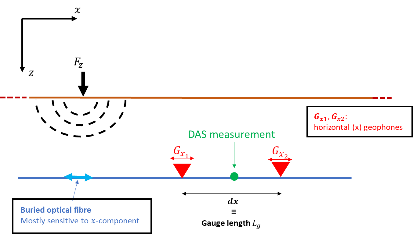
Figure 1: An illustration to compare DAS and geophone measurement.

2.2 Phase velocity retrieval

A variety of methods exist to retrieve a surface wave mode’s dispersion curve. The dispersion curve describes the mode’s phase velocity as a function of frequency. Often, dispersion curves are estimated by transforming the data into a different (spectral) domain. For example, the recorded data can be transformed from the time-space domain to the phase velocity-frequency ($c-f$; McMechan & Yedlin, 1981) domain, to the frequency-wavenumber ($f-k$; Foti et al., 2000) domain, or to the phase-offset ($\phi-x$; Strobbia & Foti, 2006) domain. These methods have in common that they rely on the assumption that the subsurface is a stack of horizontal layers. In other words, the subsurface is assumed to be laterally invariant. Consequently, in the case of laterally rapidly varying structure, the retrieved dispersion relation is effectively a (non-exact) average (Boiero & Socco, 2010). In practice, these methods are assumed still to be valid when the subsurface is laterally very smooth.

In case the subsurface is laterally invariant, the relation between the phase ($\phi$) and offset ($x$) will be linear at each discrete frequency ($f_{i}$), with the slope coinciding with the wavenumber ($k$). This can be formulated as (Strobbia & Foti, 2006):

$$\phi(f_{i},x)=k(f_{i})x+\phi_{0}(f_{i}),$$ (2)

where $\phi_{0}$ is the phase at the location of the source. Equation (2) allows the estimation of a wavenumber by means of a least-squares fit of the phase-offset data at each discrete frequency $f_{i}$, i.e., using a linear regression (for detailed formulation see Strobbia & Foti, 2006). The estimated wavenumber ($k(f_{i})$) can be translated to the frequency-dependent phase velocity ($c(f_{i})$) using:

$$c(f_{i})=\dfrac{2\pi f_{i}}{k(f_{i})},$$ (3)

where $i=1,2,...,N_{f}$, and $N_{f}$ denotes the number of discrete frequencies. This approach is referred to as the ‘Multi Offset Phase Analysis’ (MOPA; Strobbia & Foti, 2006; Vignoli & Cassiani, 2010).

In the above description, the subsurface is approximated by a single dispersion curve for the whole of $x$. In the presence of lateral variations, Equation (2) can be formulated such that the wavenumber $k$ varies as a function of both offset and frequency. That is, $k=k(f_{i},x^{\mathrm{(c)}})$, where $x^{\mathrm{(c)}}$ denotes the center position of a set of adjacent (Fourier transformed) wavefield recordings running from $x^{\mathrm{(c)}}-W/2$ to $x^{\mathrm{(c)}}+W/2$ (here, $W$ is the spatial window along which $k(f_{i},x^{\mathrm{(c)}})$ is assumed to be constant). Vignoli et al. (2011) “move” this spatial window along the recording line with small steps (i.e., significantly smaller than $W$). This is done separately for each discrete frequency, allowing $W$ to be frequency dependent (Vignoli et al., 2016). The wavenumbers are subsequently derived using linear regression according to Equation (2). These laterally varying wavenumbers are subsequently converted to laterally varying phase velocities $c(f_{i},x^{\mathrm{(c)}})$ using Equation 3. Since the lateral resolution of the surface waves is directly related to the wavelength (Barone et al., 2021), Vignoli et al. (2016) proposed to have the spatial window length $W$ be a function of the wavelength of the surface waves.

In this study, we use the MOPA algorithm of Vignoli et al. (2016) to estimate local dispersion curves. Chiefly, this is because of the algorithm’s robustness and simplicity. A drawback of the MOPA algorithm, however, is that it can only be applied to a single surface wave mode. Therefore, only one mode will be considered, and the rest of the available surface wave modes and body waves have to be filtered out. Finally, it should be understood that the recovered wavenumbers are associated with the wavefield. That is, they will deviate from the medium’s true wavenumber distribution (sometimes referred to as ‘structural wavenumbers’; Wielandt, 1993), with the discrepancy between the two being larger for more heterogeneous subsurfaces.

2.3 Transdimensional surface wave tomography

A single dispersion curve, i.e., $c(f_{i},x^{\mathrm{(c)}})$ for a specific location $x^{\mathrm{(c)}}$ (with $i=1,2,...,N_{f}$), can be “inverted” to recover a (1D) shear-wave velocity profile. Numerous inversion algorithms are described in the literature. Roughly speaking, one can distinguish between linearized algorithms (e.g., Xia et al., 1999) and nonlinear global search methods. The latter include genetic algorithms (Yamanaka & Ishida, 1996), simulated annealing (Beaty et al., 2002), the neighborhood algorithm (Wathelet, 2008), Monte Carlo methdos (Socco & Boiero, 2008), particle swarm optimization (Wilken & Rabbel, 2012), and a 1D transdimensional algorithm (Bodin et al., 2012b).

In the presence of lateral variations, the dispersion relation varies as a function of location. In that case, the different dispersion curves are often inverted independently using one of the mentioned 1D inversion algorithms (e.g., Bohlen et al., 2004; Socco et al., 2009; Vignoli et al., 2016; Barone et al., 2021), after which the independently inverted 1D profiles are pieced together to obtain a 2D (or 3D) shear-wave velocity pseudo-section (or pseudo-cube). However, by independently inverting the adjacent dispersion curves, lateral correlations in the subsurface structure are ignored (Zhang et al., 2020). Socco et al. (2009) propose to invert all dispersion curves simultaneously to mitigate the solution’s non-uniqueness, and retain lateral smoothness. They use a laterally constrained least-squares algorithm in which each 1D model is linked to its neighbors. Zhang et al. (2020) invert all dispersion curves simultaneously using a (Bayesian) 3D transdimensional algorithm. In this study, we invert all $c(f_{i},x^{\mathrm{(c)}})$ simultaneously using a 2D transdimensional algorithm (Bodin & Sambridge, 2009). As such, we retain lateral shear-wave correlations and circumvent (rather arbitrary) smoothing and damping procedures.

The 2D transdimensional tomographic algorithm by Bodin & Sambridge (2009) is originally developed for travel time tomography. Here, we modify the algorithm to invert all DAS-derived dispersion curves simultaneously. Our transdimensional algorithm uses a 2D Voronoi tessellation to parameterize the model space ($\mathbf{m}$) in combination with a reversible jump Markov chain. A Voronoi cell is defined by the location of its nucleus and the shear-wave velocity assigned to it. The geometry of each cell is controlled by its neighboring cells. Reversible jump Markov chain Monte Carlo (rjMcMC; Green, 1995) allows a variable parameterization of the model space, meaning that the number of Voronoi cells, their locations, and the assigned velocities are all unknowns (Rahimi Dalkhani et al., 2021). The transdimensional parameterization allows the algorithm to sample the full model space, without the need to introduce any kind of regularization (Bodin & Sambridge, 2009).

The rjMcMC algorithm is a Bayesian inference method that aims to sample the posterior probability density of the model parameters given the observed data, $p(\mathbf{m}|\mathbf{d})$. The posterior is proportional to the product of the likelihood $p(\mathbf{d}|\mathbf{m})$ and the prior $p(\mathbf{m})$ (Bodin & Sambridge, 2009; Rahimi Dalkhani et al., 2021):

$$p(\mathbf{m}|\mathbf{d})\propto p(\mathbf{d}|\mathbf{m})p(\mathbf{m}).$$ (4)

The prior probability distribution, $p(\mathbf{m})$, incorporates all (a priori) known independent information about the model space. Similar to Bodin & Sambridge (2009), we consider an uninformative uniform prior for all the model parameters (i.e., number of cells, Voronoi nuclei location, and velocity assigned to each cell).

The likelihood function $p(\mathbf{d}|\mathbf{m})$ plays a fundamental role in the inference of the model space as it provides the probability of the observed laterally varying dispersion curves given a specific velocity model. It is formulated as:

$$p(\mathbf{d}|\mathbf{m})=\prod_{i=1}^{N_{f}}\prod_{j=1}^{N_{x}}\bigg{(}\dfrac{1}{\sqrt{2\pi}\sigma_{ij}}\exp(-\dfrac{\big{(}g_{ij}(\mathbf{m})-d_{ij}\big{)}^{2}}{2\sigma_{ij}^{2}})\Bigg{)},$$ (5)

where $N_{x}$ is the number of locations $x_{j}^{\mathrm{(c)}}$ for which a dispersion curve is estimated (i.e., $j=1,2,...,N_{x}$). Data point ${d}_{ij}$ is the phase velocity at discrete frequency $f_{i}$ and location $x_{j}^{\mathrm{(c)}}$ (Figure 3e). The vector $\mathbf{m}$ contains the parameters describing the proposed model. Due to the variable number of Voronoi cells, its length changes while the posterior is being sampled. Furthermore, $g_{ij}$ is the modeled laterally varying phase velocity and $\sigma_{ij}$ is the data uncertainty or noise level for the phase velocity at the discrete frequency $f_{i}$ and location $x_{j}^{\mathrm{(c)}}$.

The reversible jump Markov chain draws samples from the posterior distribution by means of a Metropolis-Hasting (MH) algorithm which includes changing the dimension of the model space. Jumping between different dimensions of the model space allows the rjMcMC algorithm to perform a global search and overcome the problem of local minima (Andrieu et al., 1999). The process starts with some random initial model $\mathbf{m}$. Then, the algorithm draws the next sample of the chain by proposing a new model, $\mathbf{m}^{\prime}$, based on a known proposal probability function, $q(\mathbf{m}^{\prime}|\mathbf{m})$, which only depends on the previous state of the model $\mathbf{m}$. The proposed model $\mathbf{m}^{\prime}$ will be accepted with probability (Bodin & Sambridge, 2009):

$$\alpha(\mathbf{m^{\prime}}|\mathbf{m})=min[1,\dfrac{p(\mathbf{m^{\prime}})}{p(\mathbf{m})}\dfrac{p(\mathbf{d}|\mathbf{m^{\prime}})}{p(\mathbf{d}|\mathbf{m})}\dfrac{q(\mathbf{m}|\mathbf{m^{\prime}})}{q(\mathbf{m^{\prime}}|\mathbf{m})}\times|\mathbf{J}|],$$ (6)

where, $\dfrac{p(\mathbf{m^{\prime}})}{p(\mathbf{m})}$ is the prior ratio, $\dfrac{p(\mathbf{d}|\mathbf{m^{\prime}})}{p(\mathbf{d}|\mathbf{m})}$ is the likelihood ratio, $\dfrac{q(\mathbf{m}|\mathbf{m^{\prime}})}{q(\mathbf{m^{\prime}}|\mathbf{m})}$ is the proposal ratio, and $\mathbf{J}$ is the Jacobian of transformation from $\mathbf{m}$ to $\mathbf{m^{\prime}}$ and is needed to account for scale changes involved when the perturbation considers a jump between dimensions (Green, 1995).

The acceptance probability, $\alpha(\mathbf{m}^{\prime}|\mathbf{m})$, is the key to ensuring that the samples will be generated according to the target posterior distribution, $p(\mathbf{m}|\mathbf{d})$ (Bodin & Sambridge, 2009). Similar to Bodin & Sambridge (2009), we used four perturbation types to propose a new model ($\mathbf{m}^{\prime}$) based on the current model ($\mathbf{m}$) including nuclei move, velocity update, birth, and death steps. We followed exactly the same way as Bodin & Sambridge (2009) to parametrize the model space and perturb the model space using the four perturbation types. Consequently, the formulas to compute the acceptance probability (Equation 6) are identical to the ones derived by Bodin & Sambridge (2009).

It is worth noting that the input data in our case (i.e., laterally varying phase velocities along a 2D line) is different from the travel times used in Bodin & Sambridge (2009). Consequently, a different forward function ($g$ in Equation 5) is necessary to compute the modeled data. For this purpose, we use a MATLAB package developed by Wu et al. (2019) using the method proposed in Buchen & Ben-Hador (1996). This algorithm computes the dispersion curve (i.e., phase velocity versus frequency) in a 1D earth model. Therefore, to model the laterally varying dispersion curves, we take the 1D velocity profile at each location and compute the dispersion curves independently.

3 Application to synthetic data

In order to test the proposed workflow, we consider a 2D synthetic model with lateral variation and a low-velocity layer near the surface (Figure 2a). The wavefield is modeled using a two-dimensional finite-difference elastic wave equation solver (Thorbecke, 2017) assuming a free surface at the top of the model and a compressional (p-wave) source type. The source time function is a 12 Hz Ricker wavelet. Since the straight fibers record the radial component of the surface waves, we use the horizontal component of the wavefield recorded at the surface of the synthetic model (Figure 2b). In this experiment, the recorded surface wave on the horizontal component of the wavefield is the Rayleigh wave. We indicated the fundamental-mode surface wave (R0), higher-modes surface waves (R+), and the direct body wave (DW) on the seismic record in Figure 2b. The $f-k$ spectrum is shown in Figure 2c. The fundamental-mode Rayleigh wave is dominant in Figure 2b-d.

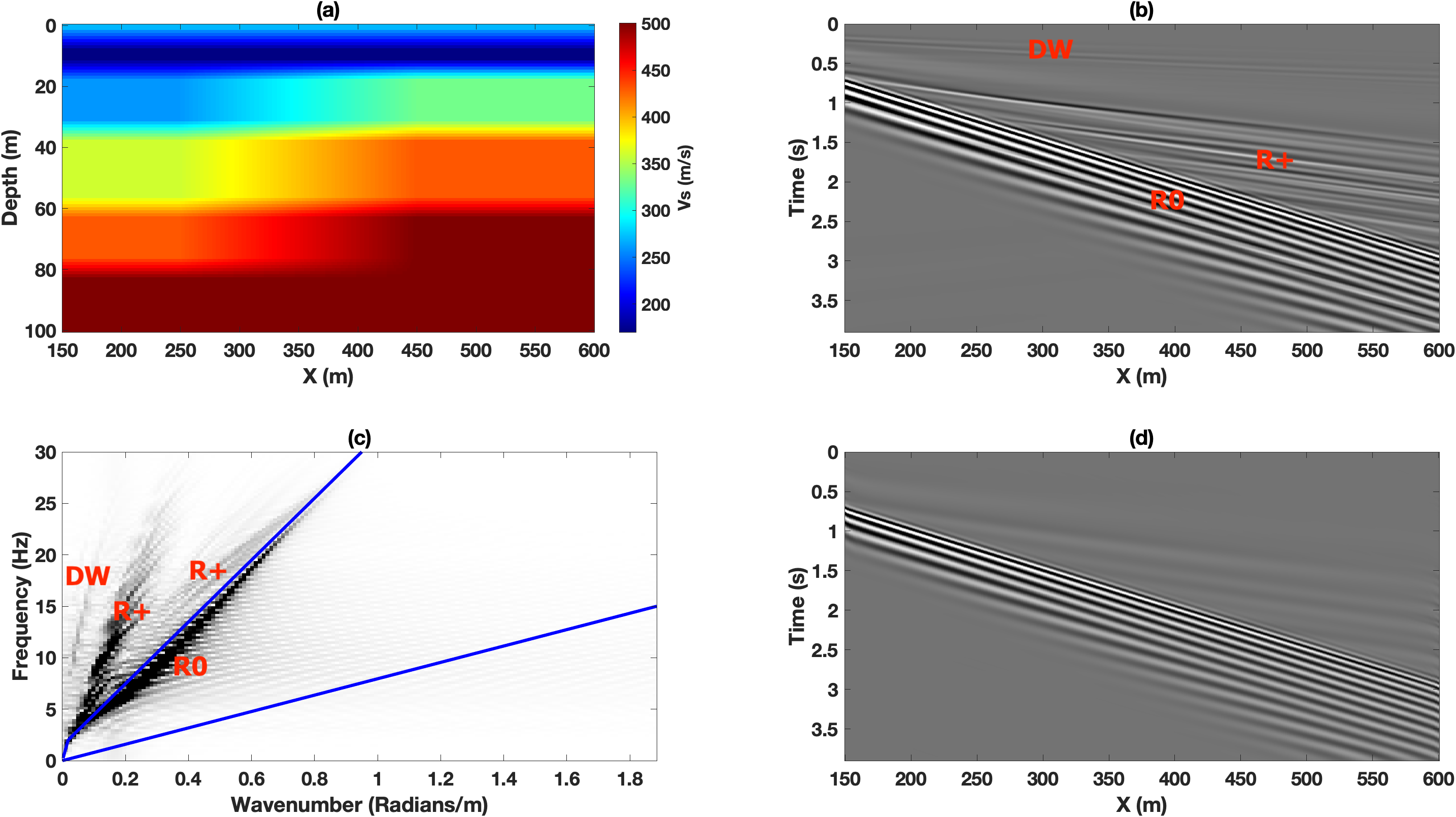
Figure 2: Surface wave spectral analysis of a synthetic active seismic record. (a) The prescribed synthetic model. (b) The horizontal component of the wavefield recorded at the surface for a source located at x = 0 m. (c) $f-k$ spectrum. fundamental-mode surface waves (R0), higher-modes surface waves (R+), and direct body waves (DW) are indicated in (b-c). (d) An isolated fundamental-mode is retained after an f-k filter has been applied. The blue lines in (c) represent the corner frequencies of the applied velocity filter.

3.1 Multi Offset Phase Analysis

To obtain a reliable phase versus offset spectrum that is associated with the fundamental-mode only, we isolate the fundamental-mode (Figure 2d) by retaining the energy contained by the blue lines in Figure 2c and muting the rest of the spectrum ($f-k$ filtering). The filtered data, after computation of the inverse transform, is presented in Figure 2d. Subsequently, each trace of the “cleaned” shot record is transformed to the frequency domain using a Fast Fourier Transform. For each discrete frequency $f_{i}$, the phases of the individual traces are unwrapped (e.g., Weemstra et al., 2021), resulting in the $\phi-x$ spectrum. The (unwrapped) phase versus offset is presented for six different frequencies in Figure 3a.

The retrieved laterally varying dispersion curves using the MOPA are depicted in Figure 3b for the single shot record of Figure 2d. Here, we used a spatial window length $W(f_{i})$ equal to two wavelengths, where the latter is computed using a reference phase velocity based on the (averaged) phase velocity retrieved through the application of MOPA to the whole shot record. This frequency dependency implies that $W$ decreases with increasing frequency. Linear regression using Equation (2) for each $f_{i}$ and $x_{j}^{\mathrm{(c)}}$ separately, subsequently results in the frequency-dependent “local” wavenumbers. These wavenumbers are then transformed into phase velocities using Equation (3), yielding the set of laterally varying dispersion curves depicted in Figure 3b.

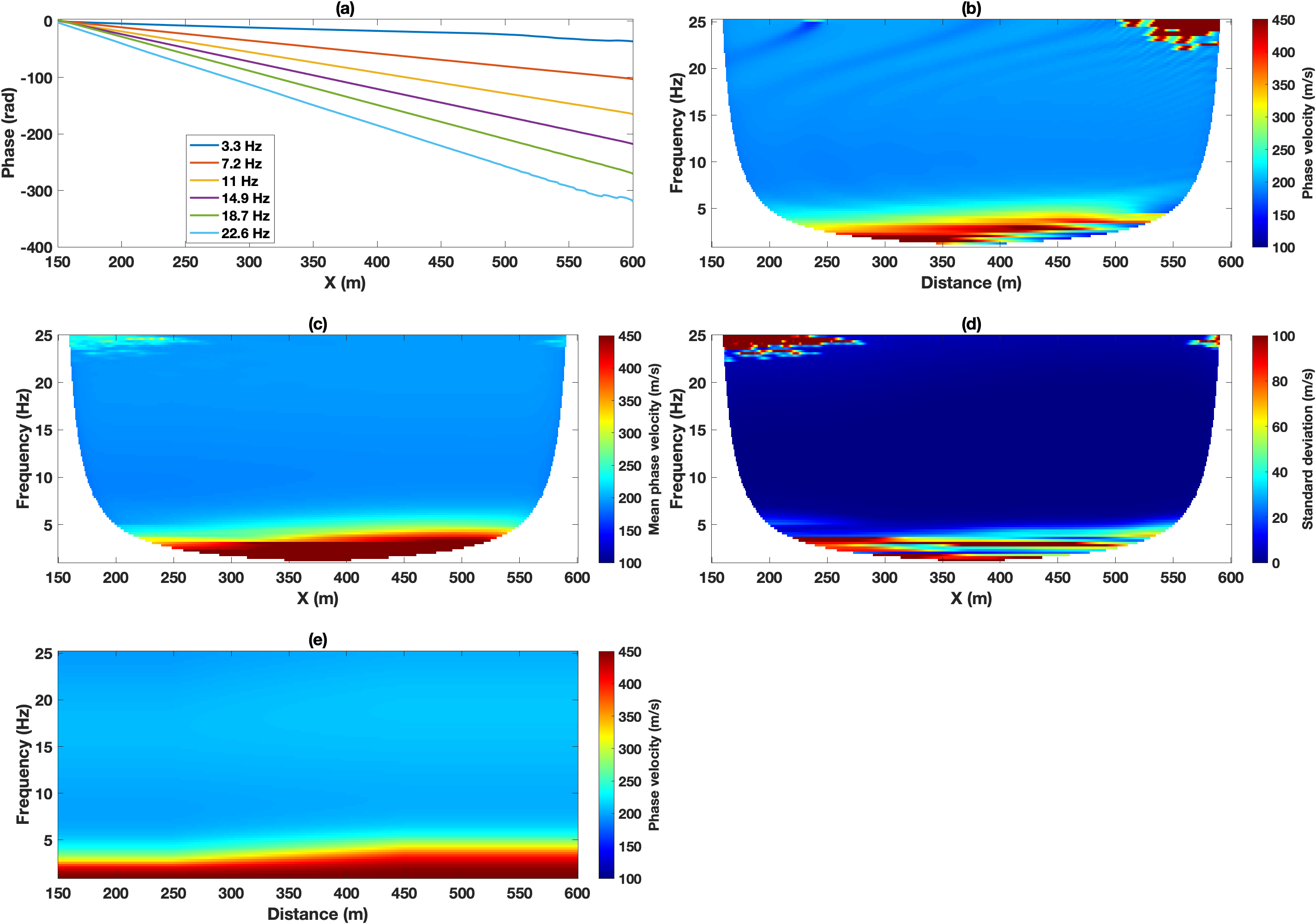
Figure 3: Phase velocity retrieval using MOPA: application to synthetic recordings. (a) Phase versus offset for six discrete frequencies of the filtered shot record presented in Figure 2d. (b) Phase velocities $c(f_{i},x_{j}^{\mathrm{(c)}})$ retrieved from one single shot record. (c) Mean local phase velocities retrieved from 32 shots. (d) Standard deviation corresponding to (c). (e) Theoretical (true) laterally varying phase velocities.

To improve the quality of the recovered dispersion curves, MOPA is conventionally applied to multiple shots, each located at a different (in-line) position. In this synthetic experiment, we modeled 32 shot records with sources located between 0-150 m and 600-750 m and with a source spacing of 10 m. Additionally, an $f-k$ filter is applied to each (Fourier transformed) shot record to facilitate a reliable phase analysis by isolating the fundamental-mode. Subsequently, laterally varying dispersion curves are estimated through the application of MOPA to each shot record separately. At each position $x_{j}^{\mathrm{(c)}}$, this results in 32 independently estimated dispersion curves. The average of these 32 sections is presented in Figure 3c. The associated standard deviation is presented in Figure 3d, which is a measure of the uncertainty of the recovered $c(f_{i},x_{j}^{\mathrm{(c)}})$.

Figure 3e shows the (true) theoretical location-dependent phase velocities as a reference. These are computed by taking the true 1D shear-wave velocity profile at each location and then computing the theoretical dispersion curve using the reduced delta matrix method (Buchen & Ben-Hador, 1996; Wu et al., 2019). Figure 3c,e show that lower frequencies (less than 3 Hz) and also higher frequencies (higher than 20 Hz) are associated with higher uncertainties and deviate from the theoretical dispersion relation. These are due to the low amplitude of the source time function (i.e., a 12 Hz Ricker) at those frequencies. Additionally, residual higher-modes (visible in Figure 2d) also affect the quality of the dispersion relation. Finally, the MOPA algorithm does not cover the regions close to the profile ends due to spatial windowing. Since this window length $W$ is larger at lower frequencies, lower frequencies sampled over a shorter spatial interval in Figure 3b,c.

3.2 Inversion

The recovered local phase velocities are now used in the proposed 2D transdimensional inversion algorithm. We used 20 independent chains to sample the posterior each sampling 700,000 models. The initial model of each chain is generated randomly with a randomly selected number of cells and a randomly chosen location. We only assumed an increasing velocity with depth for the initial model (Figure 4a). The last collected sample of that chain is shown in Figure 4b. We discarded the first 200,000 samples as the burn-in period. Then samples are retained at every 100 iterations to avoid collecting correlated samples. Consequently, a total of 100,000 samples are retained and used for the calculation of the posterior mean (Figure 4c) and the posterior standard deviation (Figure 4d).

Figure 4c shows that the proposed algorithm successfully recovered the true shear wave velocity model of Figure 2a near the surface. In deeper parts of the model, the recovered shear wave velocity is a smoother version of the true velocity model. The uncertainty presented in Figure 4d is also meaningful by having higher values in the layer interfaces.

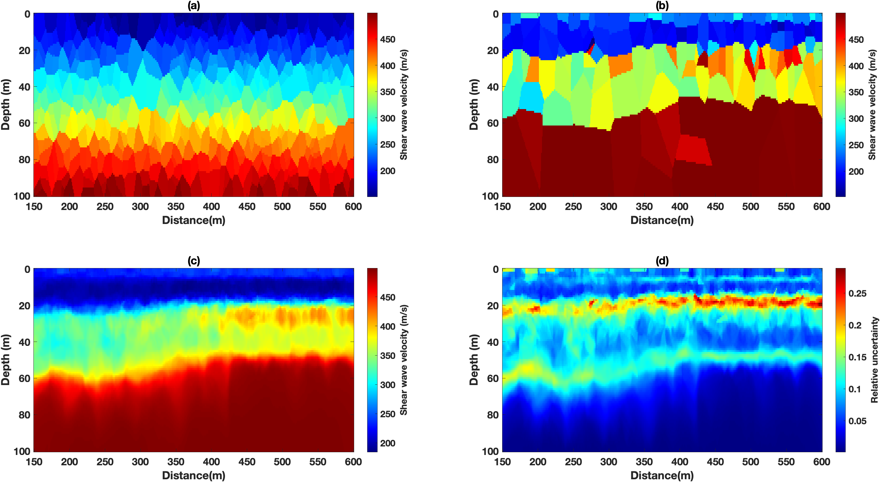
Figure 4: (a) A random initial model of a chain. (b) The last collected sample of the chain. (c) The posterior mean of the collected samples from 20 parallel chains. (d) The posterior standard deviation of the retained samples.

4 Application to DAS data recorded near Zuidbroek, Groningen

In this section, we discuss the application of the proposed methodology to a field data set recorded using a straight fiber DAS system. We first introduce the data. Then we recover the local phase velocities followed by a 2D transdimensional inversion. The results are then compared with the shear wave velocity profiles measured at two boreholes along the acquisition line.

4.1 Data characteristics

The proposed methodology has been applied to data obtained in the area of Groningen in the north of The Netherlands. These data were obtained with fibers as part of a Distributed Acoustic Sensing (DAS) system. Figure 3 shows the acquisition setup of the DAS system. Figure 5 shows the acquisition setup of the DAS recording system. Several configurations of fibers were used, namely straight and helically wound fibers during the recording (Al Hasani & Drijkoningen, 2023), however, we opted for the straight fiber data as it showed the highest sensitivity to the surface waves. The source used is an electrically driven vertical seismic vibrator (Noorlandt et al., 2015) shooting 2 shots per position from x=0 to x=750 every 2 m. The straight fiber is buried 2m in depth with a length of 450 m from x = 150-600. More information on the acquisition can be found in Al Hasani & Drijkoningen (2023).

The receiver spacing of the recordings is 1 m with a gauge length of 2 m. We considered 152 off-end shots on the two sides of the recording line for the application of MOPA. In fact, for the purpose of surface wave analysis and inversion, all shots located at x = 0-150 m and x = 600-750 m are considered in this study, a total of 152 shots.

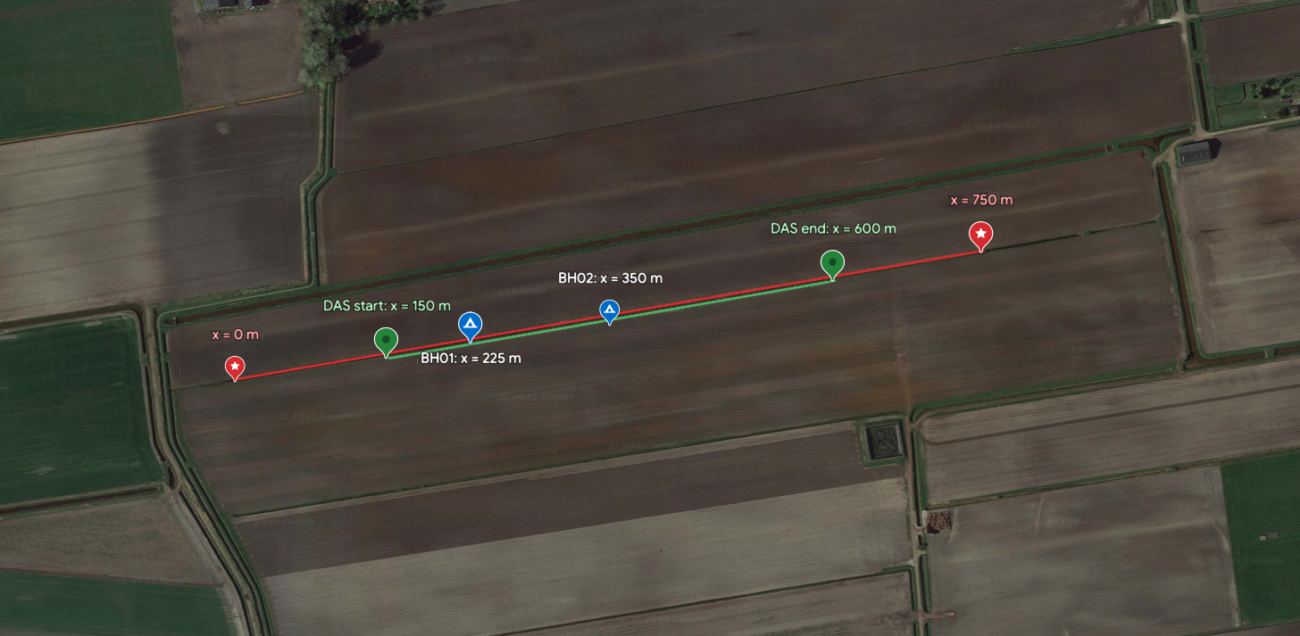
Figure 5: The acquisition setup of the recorded DAS data in the Groningen area. The red line shows the source line with a length of 750 m and a source spacing of 2 m. The green line shows the DAS straight fiber buried 2 m in depth and with a length of 450 m. The start of the source line is marked as x = 0 and the end of the source line is marked as x = 750 m. The DAS fiber is also located at x = 150 - 600 m. Two boreholes are also drilled to a depth of 80 m at x = 225 m and x = 350 m to measure the shear-wave velocity directly.

Figure 6 shows a sample shot gather of the DAS data recorded at a farm in the Groningen area, the Netherlands. The $f-k$ and $c-f$ spectra are also provided for a better understanding of the data. First, a straight fiber records the radial component of the wave field. Since the vertical source is in line with the fiber (i.e., receivers), the recorded surface wave in the radial direction is the Rayleigh wave. Second, the shot record is dominated by the fundamental-mode Rayleigh wave indicated by R0. The fundamental-mode is easily detectable in the frequency range of 4-20 Hz in both $f-k$ and $c-f$ spectra. Third, higher-modes are also clearly visible in both shot records and their corresponding spectra. We have indicated higher-modes by R+ since more than one higher-mode is visible in the $f-k$ and $c-f$ spectra; it is also difficult to separate them. Finally, the colored lines in the $f-k$ spectra represent phase velocities to design a velocity filter for isolating the fundamental-mode. The velocity lines are also depicted on the $c-f$ spectra for the reader’s reference. As you can see, the red line separating the fundamental-mode from higher-modes is velocity dependent. The $f-k$ spectrum between the blue and the red line is preserved and the rest of the spectrum is filtered out. The filtered record is presented in Figure 6d representing the fundamental-mode Rayleigh wave. We have applied this velocity filter to all the shots.

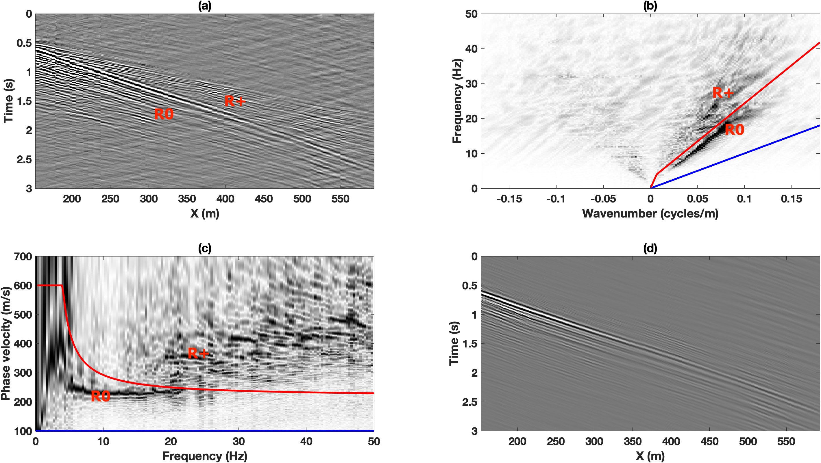
Figure 6: A common shot record (a), its corresponding f-k amplitude spectrum (b), and its corresponding dispersion image (c). The source is located at x = 10 m. The fundamental-mode and higher-modes are indicated by R0 and R+, respectively. The blue line indicates the phase velocity of 100 m/s and the red line indicates a frequency-dependent phase velocity between 220-600 m/s. (d) fundamental-mode surface wave shot records corresponding to the shots depicted in (a). An f-k filter is applied to the shot records by keeping the f-k spectrum between the blue and red lines. The rest of the spectrum is filtered out.

4.2 Multi Offset Phase Analysis

After isolating the fundamental-mode (Figure 6d), we applied the MOPA algorithm to all 152 off-end shot records of the available DAS data. Figure 7 shows the results of the MOPA method applied to the field DAS data to retrieve the dispersion curves. The unwrapped phase versus offsets for 7 frequency components of a single shot record (Figure 6b) are depicted in Figure 7a. The retrieved laterally varying dispersion curves are presented in Figure 7b, which are somehow noisy with rather sharp changes. A more smooth and more reliable dispersion curve can be derived by repeating the process for multiple shot records. Figure 7c presents the average laterally varying dispersion curves derived from 152 shot records. The uncertainty (i.e., standard deviation) is also depicted in Figure 7d.

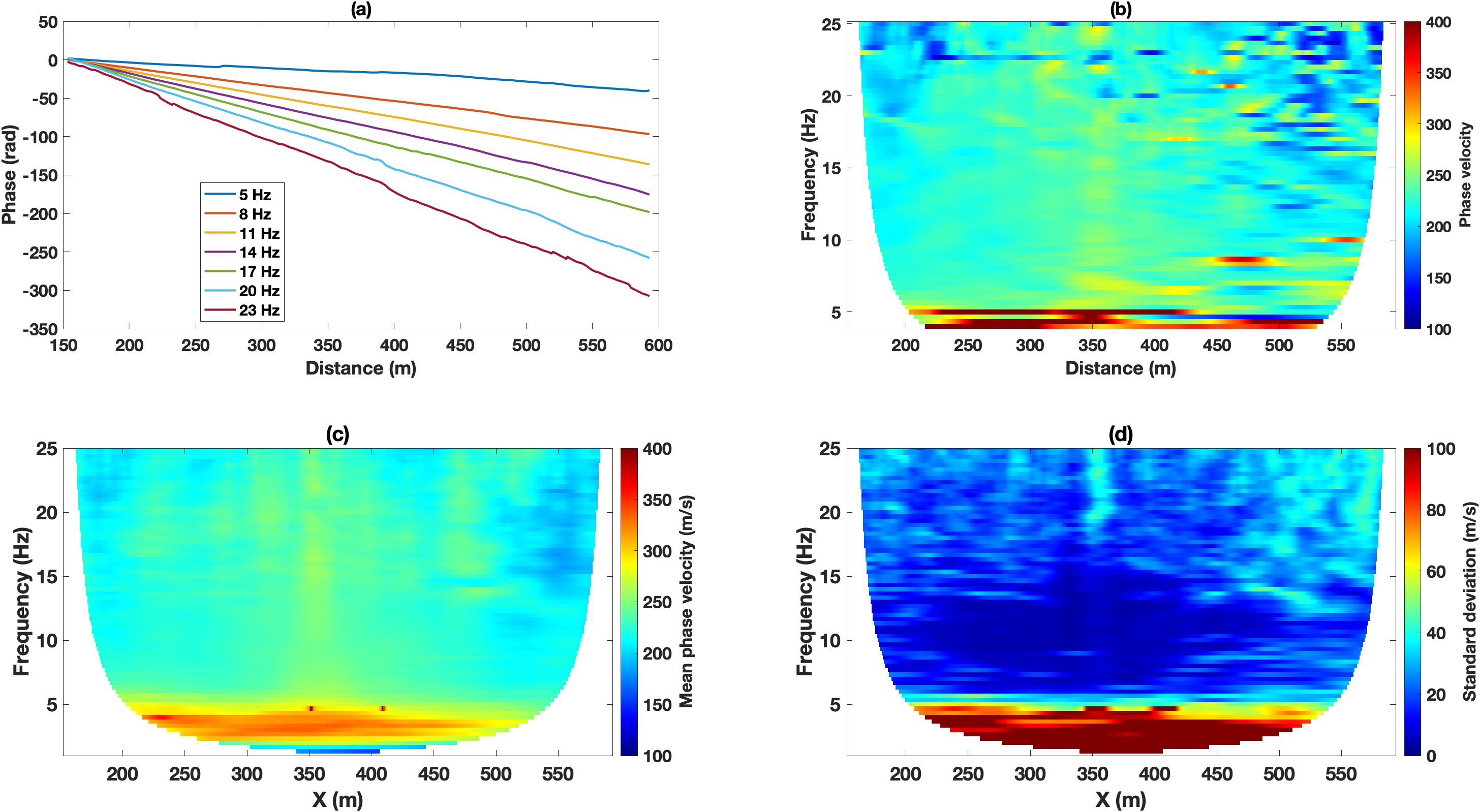
Figure 7: MOPA applied to the field DAS data considering the lateral variation of the subsurface. (a) Unwrapped phase versus offset at seven different frequencies (i.e., different colors) for the filtered seismic record depicted in Figure 6d. (b) laterally varying phase velocity retrieved from the single shot record of Figure 6d. (c) Mean of the laterally varying dispersion curves retrieved from 152 off-end shots. (d) Standard deviation corresponding to (c).

4.3 Prior information

Prior information is the known information from the area of study based on the possible previous studies or the direct measurement of the subsurface properties. In this study, two open boreholes were drilled down to a depth of 80 m, where the shear-wave velocity and p-wave velocity were measured directly using a PS suspension logging tool. In addition to the seismic data, the bulk electrical conductivity and the gamma radiation were also measured. The measured logs are presented in Figure 8. The main feature observable from the logs is a clear reduction of shear-wave velocity between 10 and 20 m, especially in Figure 8(a). This is due to the higher clay content supported by the conductivity and gamma-ray values having higher values than above and below that layer. In addition, the relatively low electrical conductivity values indicate fresh water and the relatively low gamma ray values indicate a low level of clay content. Consequently, the top 10 m of the subsurface is predominantly sand with fresh water.

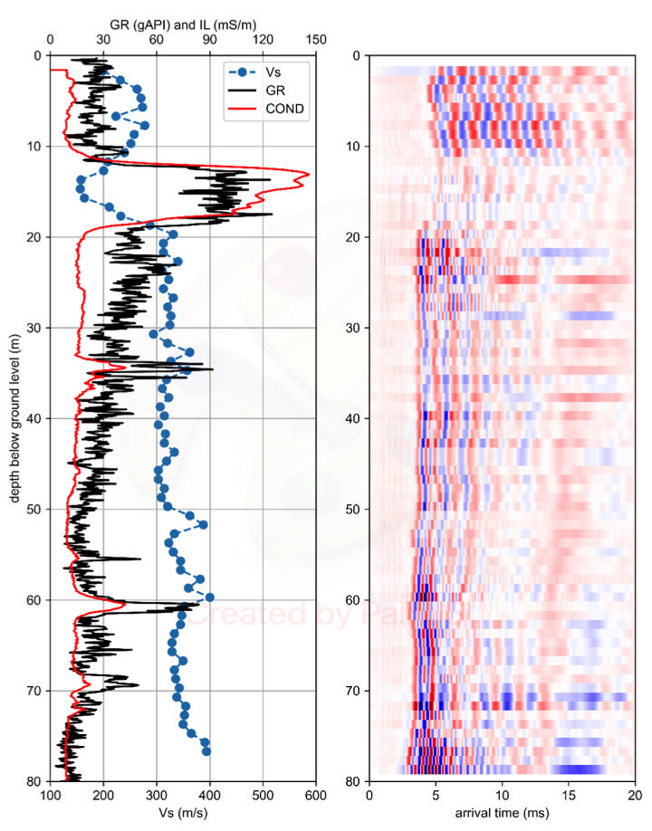
(a) BH01

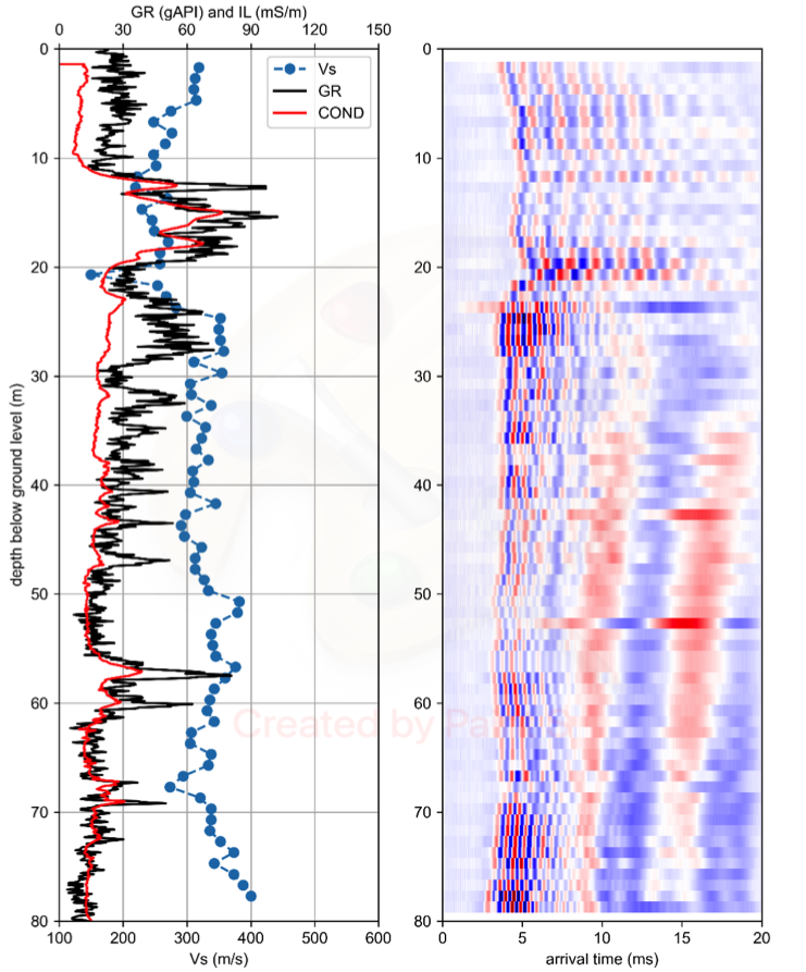
(b) BH02

Figure 8: The measured Induction-Log readings (IL), Gamma Ray (GR), and shear-wave velocity profile ($V_{s}$) together with the far receiver s-wave seismogram of (a) first borehole (BH01) at x = 220 m and (b) second borehole (BH02) at x = 350 m of the recording line.

This logging information can be used to construct a prior probability distribution for the shear-wave velocity, which is the subject of another study. In this study, we assumed an uninformative uniform prior distribution for the shear-wave velocity with the prior bounds of 50-600 m/s, and we used these logging data to validate our inversion results. Additionally, to compute the surface wave dispersion curves theoretically, we need the shear-wave velocity ($V_{s}$), p-wave velocity($V_{p}$), and density ($\rho$). However, the shear-wave velocity is mainly controlling the theoretical dispersion curves, and the effect of $V_{p}$ and $\rho$ is ignored in the literature Wathelet (2008). We used the logging data to get an estimate of the $\dfrac{V_{p}}{V_{s}}$ ratio to be used in the theoretical calculation of the dispersion curves. To that end, we first smoothed the shear-wave velocity profile (Figure 9a) and the compressional-wave velocity profile (Figure 9b) using a moving average profile. Then, a depth-dependent $\dfrac{V_{p}}{V_{s}}$ ratio is computed based on the smoothed blue curves presented in Figure 9c. During the inversion process, we used a $\dfrac{V_{p}}{V_{s}}$ ratio of 5 to relate the shear-wave velocity and the compressional-wave velocity while computing the dispersion curves.

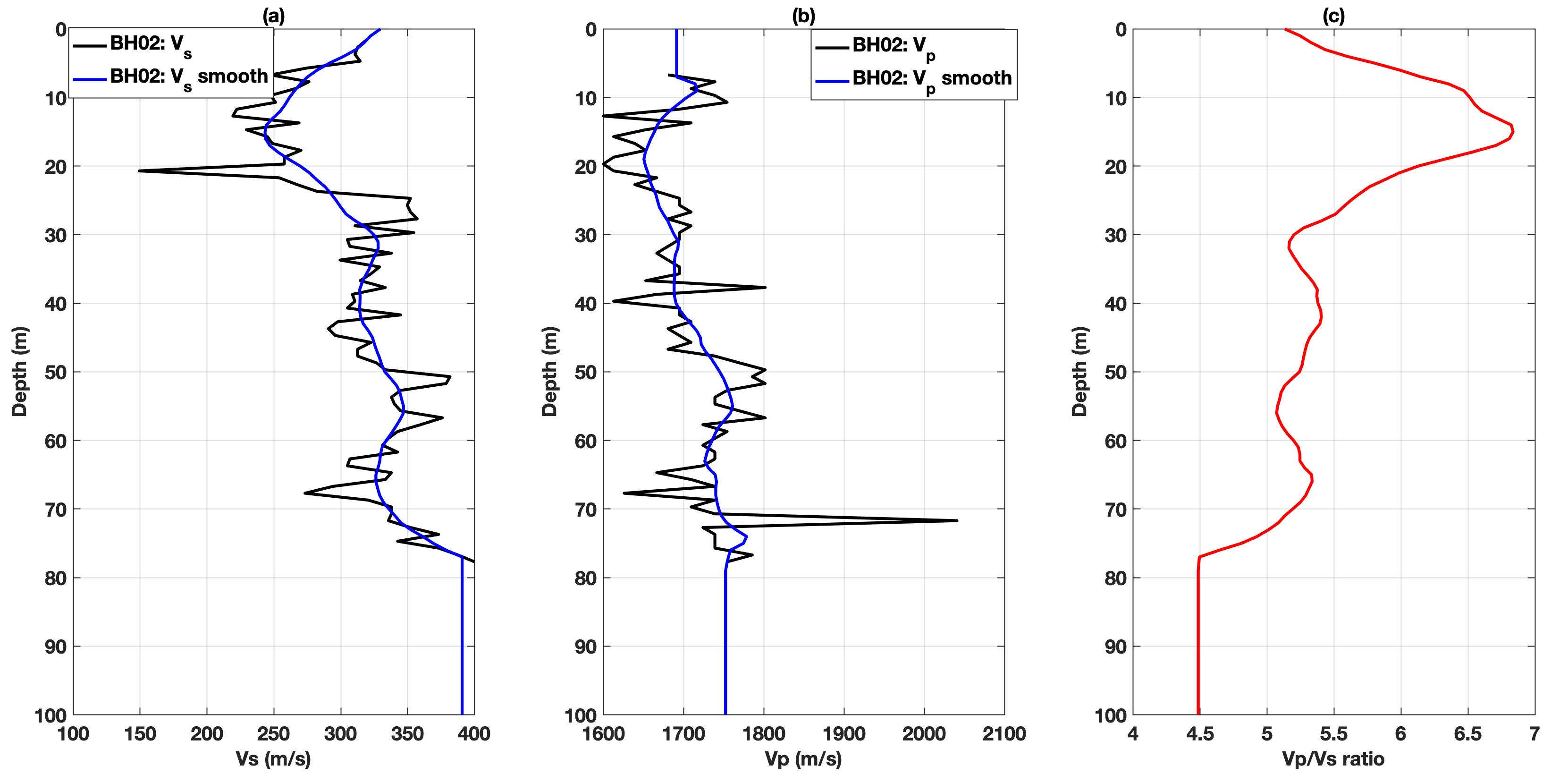
Figure 9: shear-wave velocity profile (a) and p-wave velocity profile (b) measured at the second borehole (BH02). The blue curves are the smooth version of the original velocity profiles using a moving average filter. (c) The $\dfrac{V_{p}}{V_{s}}$ ratio is computed based on the smooth blue curves.

s

4.4 Transdimensional inversion

The retrieved laterally varying phase velocities (Figure 7e) are now used in the 2D transdimensional algorithm. We used 20 independent McMC chains running in parallel each sampling 700,000 models. The initial model at each chain is selected randomly with velocity increasing with depth. The first 200,000 samples of each chain are discarded as the burn-in phase. To avoid correlated samples, the samples are retained after every 100 iterations of the McMC. Consequently, a total of 100,000 retained samples are used as the representation of the posterior distribution to compute the posterior mean (i.e., posterior expectation) and standard deviation (i.e., posterior uncertainty).

Figure 10 presents the recovered shear-wave velocity profile using the 2D transdimensional method. The shear-wave velocity profiles from the well logs are also compared with the transdimensional inverted result. As one can see, the inverted shear-wave velocity is in good agreement with the well log data at the location of the second borehole (i.e., x = 350 m). The inverted result follows the well log data and the main anomalies are resolved. At the location of the first borehole (i.e., x = 220 m), the inverted shear-wave velocity deviates a bit more from the well log data while predicting the low velocity anomaly between the depth of 10-20 m. This deviation at the location of the first borehole is mainly due to the lower quality of the MOPA derived dispersion curves. As one can see in Figure 7e-f, the retrieved phase velocity at the sides of the model has fewer frequency components and is associated with higher uncertainties.

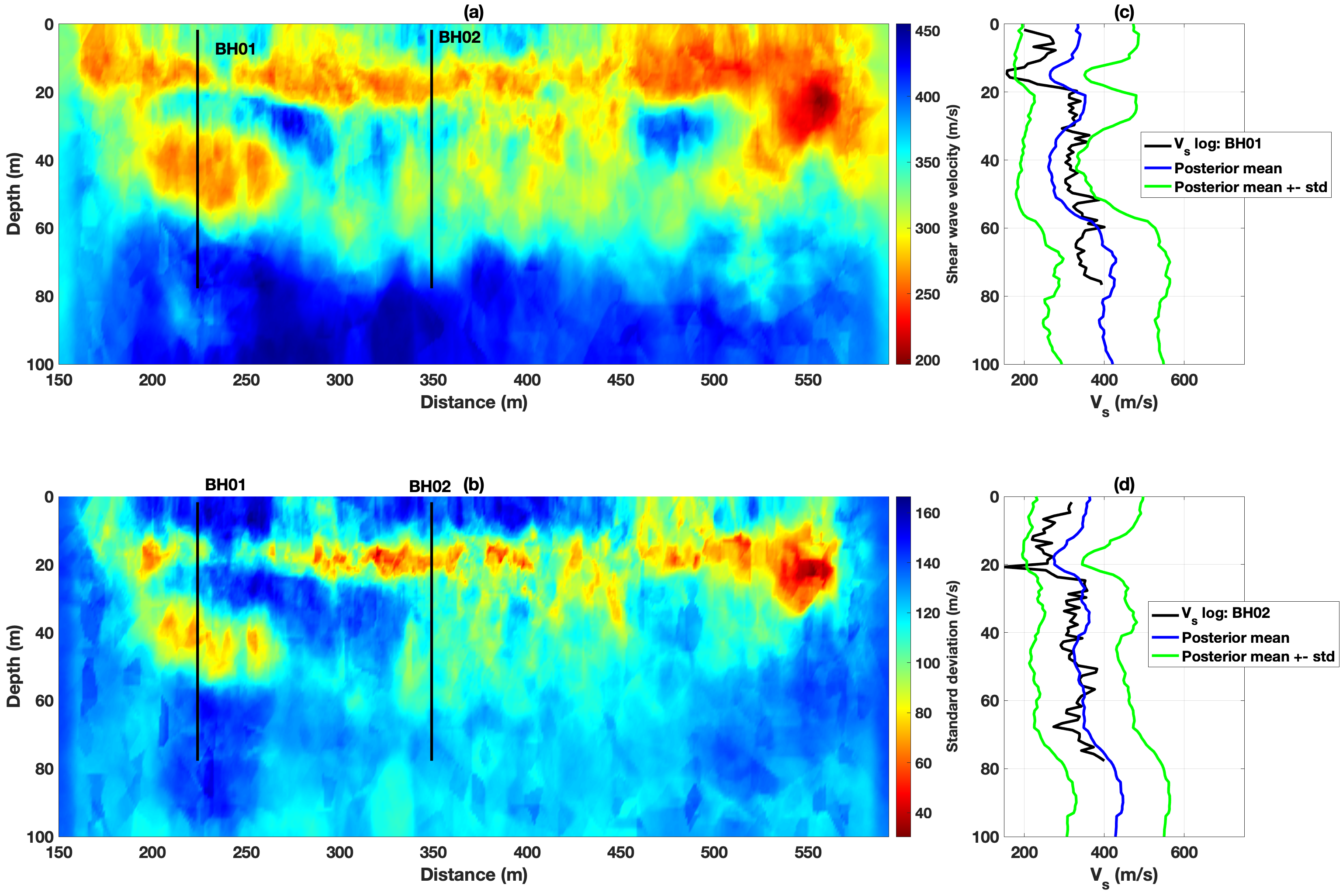
Figure 10: 2D transdimensional inversion results. (a) Recovered shear-wave velocity 2D section (i.e., posterior mean), (b) recovered model uncertainty (i.e., posterior standard deviation) and comparison with the shear-wave velocity profile available from the first borehole (c) and the second borehole (d).

5 Discussion

There are several points of discussion. First, the agreement between the transdimensional derived shear-wave velocity and the well logs are promising, especially at the location of the second borehole close to the middle of the seismic line. However, at the location of the first borehole where the retrieved phase velocity is missing lower frequencies and associated with higher uncertainties, the results deviate from the more reliable and locally measured log model. This is due to the MOPA algorithm we used in this study. The quality of the dispersion curves at these locations might be improved by the tomography-derived phase velocity retrieval algorithm (Barone et al., 2021).

Second, data uncertainty ($\sigma$ in Equation 5) plays a crucial role in the convergence of a Bayesian algorithm (Bodin et al., 2012a; Rahimi Dalkhani et al., 2021). As discussed earlier, the MOPA algorithm we used in this study provides us with an estimate of the data uncertainty (Figure 3f). In this study, we used this MOPA-derived uncertainty during the McMC sampling of the posterior. However, modeling and other processing errors are also affecting Bayesian inference. Consequently, we suggest further studies to take into account these errors to improve the convergence of each sampling chain and to enhance the quality of the final inversion result.

Third, the proposed 2D transdimensional algorithm is comparable with the independent 1D inversion of the dispersion curves in terms of computational time This is because in the proposed 2D transdimensional algorithm, at each step of the McMC, we perturb a small portion of the model space. Then, we compute the forward function (i.e., the primary source of the computational demand) only at the updated part of the model space. This reduces the computational time significantly. The added values of the proposed 2D transdimensional scheme are the enhanced lateral correlation and the reduced solution nonuniqueness.

Finally, we assumed a uniform prior whereas we have two boreholes across the line measuring the shear-wave velocity directly. Using this kind of available prior data can improve the inversion result significantly.

6 Conclusion

We investigated the potential of straight fiber DAS data in combination with a 2D transdimensional inversion algorithm to recover a 2D reliable shear-wave velocity section. We successfully recovered the laterally varying phase velocities using Multi Offset Phase Analysis. Then, we adopted the 2D transdimensional algorithm to invert all the available laterally varying dispersion curves simultaneously. The recovered shear-wave velocity is smooth with imaging of the lateral variation of the near-surface. The inverted shear-wave velocity section indicates a low-velocity anomaly between 10-20 m depth which is in agreement with the shear-wave velocity logs. The low velocity is due to the high content of clay supported by gamma-ray measurements. In general, the recovered shear-wave velocity section matches the log at the second borehole at 10-65 m depth. Therefore, we were able to retrieve the lateral variability of the subsurface using Rayleigh waves, with a good match with the S-wave logs in two boreholes.

References

- Ajo-Franklin et al. (2019) Ajo-Franklin, J. B., Dou, S., Lindsey, N. J., Monga, I., Tracy, C., Robertson, M., Rodriguez Tribaldos, V., Ulrich, C., Freifeld, B., Daley, T., et al., 2019. Distributed acoustic sensing using dark fiber for near-surface characterization and broadband seismic event detection, Scientific reports, 9(1), 1328.
- Aki & Richards (2002) Aki, K. & Richards, P. G., 2002. Quantitative Seismology, University Science Books, Sausalito, California, Medium: Hardcover.
- Al Hasani & Drijkoningen (2023) Al Hasani, M. & Drijkoningen, G., 2023. Experiences with distributed acoustic sensing using both straight and helically wound fibers in surface-deployed cables–a case history in groningen, the netherlands, arXiv preprint arXiv:2304.04384.
- Andrieu et al. (1999) Andrieu, C., de Freitas, J., & Doucet, A., 1999. Robust full bayesian methods for neural networks, Advances in neural information processing systems, 12.
- Barone et al. (2021) Barone, I., Boaga, J., Carrera, A., Flores-Orozco, A., & Cassiani, G., 2021. Tackling lateral variability using surface waves: A tomography-like approach, Surveys in Geophysics, 42, 317–338.
- Beaty et al. (2002) Beaty, K. S., Schmitt, D. R., & Sacchi, M., 2002. Simulated annealing inversion of multimode rayleigh wave dispersion curves for geological structure, Geophysical Journal International, 151(2), 622–631.
- Bodin & Sambridge (2009) Bodin, T. & Sambridge, M., 2009. Seismic tomography with the reversible jump algorithm, Geophysical Journal International, 178(3), 1411–1436.
- Bodin et al. (2012a) Bodin, T., Sambridge, M., Rawlinson, N., & Arroucau, P., 2012a. Transdimensional tomography with unknown data noise, Geophysical Journal International, 189(3), 1536–1556.
- Bodin et al. (2012b) Bodin, T., Sambridge, M., Tkalčić, H., Arroucau, P., Gallagher, K., & Rawlinson, N., 2012b. Transdimensional inversion of receiver functions and surface wave dispersion, Journal of geophysical research: solid earth, 117(B2).
- Bohlen et al. (2004) Bohlen, T., Kugler, S., Klein, G., & Theilen, F., 2004. 1.5 d inversion of lateral variation of scholte-wave dispersion, Geophysics, 69(2), 330–344.
- Boiero & Socco (2010) Boiero, D. & Socco, L. V., 2010. Retrieving lateral variations from surface wave dispersion curves, Geophysical prospecting, 58(6), 977–996.
- Bostick III (2000) Bostick III, F., 2000. Field experimental results of three-component fiber-optic seismic sensors, in SEG Technical Program Expanded Abstracts 2000, pp. 21–24, Society of Exploration Geophysicists.
- Buchen & Ben-Hador (1996) Buchen, P. & Ben-Hador, R., 1996. Free-mode surface-wave computations, Geophysical Journal International, 124(3), 869–887.
- Daley et al. (2016) Daley, T. M., Miller, D. E., Dodds, K., Cook, P., & Freifeld, B. M., 2016. Field testing of modular borehole monitoring with simultaneous distributed acoustic sensing and geophone vertical seismic profiles at citronelle, alabama, Geophysical Prospecting, 64, 1318–1334.
- Dettmer et al. (2012) Dettmer, J., Molnar, S., Steininger, G., Dosso, S. E., & Cassidy, J. F., 2012. Trans-dimensional inversion of microtremor array dispersion data with hierarchical autoregressive error models, Geophysical Journal International, 188(2), 719–734.
- Foti et al. (2000) Foti, S., Lancellotta, R., Sambuelli, L., Socco, L. V., et al., 2000. Notes on fk analysis of surface waves.
- Ghalenoei et al. (2022) Ghalenoei, E., Dettmer, J., Ali, M. Y., & Kim, J. W., 2022. Trans-dimensional gravity and magnetic joint inversion for 3-d earth models, Geophysical Journal International, 230(1), 363–376.
- Green (1995) Green, P. J., 1995. Reversible jump markov chain monte carlo computation and bayesian model determination, Biometrika, 82(4), 711–732.
- Johannessen et al. (2012) Johannessen, K., Drakeley, B., & Farhadiroushan, M., 2012. Distributed acoustic sensing-a new way of listening to your well/reservoir, in SPE Intelligent Energy International, OnePetro.
- Luo et al. (2008) Luo, Y., Xia, J., Liu, J., Xu, Y., & Liu, Q., 2008. Generation of a pseudo-2d shear-wave velocity section by inversion of a series of 1d dispersion curves, Journal of Applied Geophysics, 64(3-4), 115–124.
- McMechan & Yedlin (1981) McMechan, G. A. & Yedlin, M. J., 1981. Analysis of dispersive waves by wave field transformation, Geophysics, 46(6), 869–874.
- Molenaar et al. (2012) Molenaar, M. M., Hill, D. J., Webster, P., Fidan, E., & Birch, B., 2012. First downhole application of distributed acoustic sensing for hydraulic-fracturing monitoring and diagnostics, SPE Drilling & Completion, 27(01), 32–38.
- Nayak et al. (2021) Nayak, A., Ajo-Franklin, J., et al., 2021. Measurement of surface-wave phase-velocity dispersion on mixed inertial seismometer–distributed acoustic sensing seismic noise cross-correlations, Bulletin of the Seismological Society of America, 111(6), 3432–3450.
- Neducza (2007) Neducza, B., 2007. Stacking of surface waves, Geophysics, 72(2), V51–V58.
- Noorlandt et al. (2015) Noorlandt, R., Drijkoningen, G., Dams, J., & Jenneskens, R., 2015. A seismic vertical vibrator driven by linear synchronous motors, Geophysics, 80(2), EN57–EN67.
- Park et al. (1999) Park, C. B., Miller, R. D., & Xia, J., 1999. Multichannel analysis of surface waves, Geophysics, 64(3), 800–808.
- Qu et al. (2023) Qu, L., Dettmer, J., Hall, K., Innanen, K. A., Macquet, M., & Lawton, D. C., 2023. Trans-dimensional inversion of multimode seismic surface wave data from a trenched distributed acoustic sensing survey, Geophysical Journal International, p. ggad112.
- Rahimi Dalkhani et al. (2021) Rahimi Dalkhani, A., Zhang, X., & Weemstra, C., 2021. On the potential of 3d transdimensional surface wave tomography for geothermal prospecting of the reykjanes peninsula, Remote Sensing, 13(23), 4929.
- Schaefer et al. (2011) Schaefer, J. F., Boschi, L., & Kissling, E., 2011. Adaptively parametrized surface wave tomography: methodology and a new model of the European upper mantle, Geophysical Journal International, 186(3), 1431–1453, Publisher: Blackwell Publishing Ltd.
- Socco & Boiero (2008) Socco, L. V. & Boiero, D., 2008. Improved monte carlo inversion of surface wave data, Geophysical Prospecting, 56(3), 357–371.
- Socco et al. (2009) Socco, L. V., Boiero, D., Foti, S., & Wisén, R., 2009. Laterally constrained inversion of ground roll from seismic reflection records, Geophysics, 74(6), G35–G45.
- Socco et al. (2010) Socco, L. V., Foti, S., & Boiero, D., 2010. Surface-wave analysis for building near-surface velocity models—established approaches and new perspectives, Geophysics, 75(5), 75A83–75A102.
- Strobbia & Foti (2006) Strobbia, C. & Foti, S., 2006. Multi-offset phase analysis of surface wave data (mopa), Journal of Applied Geophysics, 59(4), 300–313.
- Thorbecke (2017) Thorbecke, J., 2017. 2d finite-difference wavefield modelling, Delft University.
- Vantassel et al. (2022) Vantassel, J. P., Cox, B. R., Hubbard, P. G., & Yust, M., 2022. Extracting high-resolution, multi-mode surface wave dispersion data from distributed acoustic sensing measurements using the multichannel analysis of surface waves, Journal of Applied Geophysics, 205, 104776.
- Vignoli & Cassiani (2010) Vignoli, G. & Cassiani, G., 2010. Identification of lateral discontinuities via multi-offset phase analysis of surface wave data, Geophysical Prospecting, 58(3), 389–413.
- Vignoli et al. (2011) Vignoli, G., Strobbia, C., Cassiani, G., & Vermeer, P., 2011. Statistical multioffset phase analysis for surface-wave processing in laterally varying media, Geophysics, 76(2), U1–U11.
- Vignoli et al. (2016) Vignoli, G., Gervasio, I., Brancatelli, G., Boaga, J., Della Vedova, B., & Cassiani, G., 2016. Frequency-dependent multi-offset phase analysis of surface waves: an example of high-resolution characterization of a riparian aquifer, Geophysical Prospecting, 64(1), 102–111.
- Wathelet (2008) Wathelet, M., 2008. An improved neighborhood algorithm: parameter conditions and dynamic scaling, Geophysical Research Letters, 35(9).
- Weemstra et al. (2021) Weemstra, C., de Laat, J. I., Verdel, A., & Smets, P., 2021. Systematic recovery of instrumental timing and phase errors using interferometric surface waves retrieved from large-N seismic arrays, Geophysical Journal International, 224, 1028–1055, Publisher: Oxford University Press.
- Wielandt (1993) Wielandt, E., 1993. Propagation and structural interpretation of non-plane waves, Geophysical Journal International, 113(1), 45–53, ISBN: 0956-540X.
- Wilken & Rabbel (2012) Wilken, D. & Rabbel, W., 2012. On the application of particle swarm optimization strategies on scholte-wave inversion, Geophysical Journal International, 190(1), 580–594.
- Wu et al. (2019) Wu, D., Wang, X., Su, Q., & Zhang, T., 2019. A matlab package for calculating partial derivatives of surface-wave dispersion curves by a reduced delta matrix method, Applied Sciences, 9(23), 5214.
- Xia et al. (1999) Xia, J., Miller, R. D., & Park, C. B., 1999. Estimation of near-surface shear-wave velocity by inversion of rayleigh waves, Geophysics, 64(3), 691–700.
- Yamanaka & Ishida (1996) Yamanaka, H. & Ishida, H., 1996. Application of genetic algorithms to an inversion of surface-wave dispersion data, Bulletin of the Seismological Society of America, 86(2), 436–444.
- Yao et al. (2023) Yao, H., Ren, Z., Tang, J., Guo, R., & Yan, J., 2023. Trans-dimensional bayesian joint inversion of magnetotelluric and geomagnetic depth sounding responses to constrain mantle electrical discontinuities, Geophysical Journal International, 233(3), 1821–1846.
- Yust et al. (2023) Yust, M. B., Cox, B. R., Vantassel, J. P., Hubbard, P. G., Boehm, C., & Krischer, L., 2023. Near-surface 2d imaging via fwi of das data: An examination on the impacts of fwi starting model, Geosciences, 13(3), 63.
- Zhang et al. (2020) Zhang, X., Hansteen, F., Curtis, A., & De Ridder, S., 2020. 1-d, 2-d, and 3-d monte carlo ambient noise tomography using a dense passive seismic array installed on the north sea seabed, Journal of Geophysical Research: Solid Earth, 125(2), e2019JB018552.
- Zulic et al. (2022) Zulic, S., Sidenko, E., Yurikov, A., Tertyshnikov, K., Bona, A., & Pevzner, R., 2022. Comparison of amplitude measurements on borehole geophone and das data, Sensors, 22.