Optical color of Type Ib and Ic supernovae and implications for their progenitors

Abstract

Type Ib and Ic supernovae (SNe Ib/Ic) originate from hydrogen-deficient massive star progenitors, of which the exact properties are still much debated. Using the SN data in the literature, we investigate the optical $B-V$ color of SNe Ib/Ic at the $V-$band peak and show that SNe Ib are systematically bluer than SNe Ic. We construct SN models from helium-rich and helium-poor progenitors of various masses using the radiation hydrodynamics code STELLA and discuss how the $B-V$ color at the $V-$band peak is affected by ⁵⁶Ni to ejecta mass ratios, ⁵⁶Ni mixing and presence/absence of the helium envelope. We argue that the dichotomy in the amounts of helium in the progenitors plays the primary role in making the observed systematic color difference at the optical peak, in favor of the most commonly invoked SN scenario that SNe Ib and SNe Ic progenitors are helium-rich and helium-poor, respectively.

1 Introduction

How different are Type Ib and Type Ic supernova (SN Ib/Ic) progenitors from each other? The absence of any noticeable hydrogen lines in SNe Ib/Ic spectra implies that the hydrogen envelope of their progenitors is stripped off because hydrogen cannot be easily hidden in the spectra even for a small amount (e.g., Dessart et al., 2011). However, the absence of He I lines in SNe Ic spectra does not necessarily mean that their progenitors lack the helium envelope. The formation of He I lines requires non-thermal processes (Lucy, 1991) and a large amount of helium could be easily hidden in the spectra if radioactive ⁵⁶Ni were not present in the helium-rich layer in the SN ejecta (e.g., Dessart et al., 2012). This makes it difficult to observationally constrain the amount of helium retained in SN Ic progenitors, obstructing our comprehensive understanding of different evolutionary channels towards SNe Ib/Ic (Yoon, 2015, 2017).

Several authors have calculated SN Ib/Ic spectra from stripped-envelope progenitors having different chemical compositions (i.e., different amounts of helium and various degrees of ⁵⁶Ni mixing; Dessart et al. 2012, 2015, 2020; Hachinger et al. 2012; Teffs et al. 2020; Williamson et al. 2020). These studies indicate that while a large amount of helium ($M>\sim 1.0M_{\odot}$) can be hidden at around the optical peak without the presence of radioactive ⁵⁶Ni in the helium-rich layer (see Dessart et al., 2012), only a small amount ($M\sim 0.1M_{\odot}$, depending on the ejecta mass) can lead to formation of strong He I lines if ⁵⁶Ni is sufficiently mixed into the helium-rich layer.

Recent analyses of a large set of SNe Ib/Ic spectra seem to imply distinct progenitor chemical compositions. For example, a stronger and broader O I $\lambda 7774$ absorption line and a broader Fe II $\lambda 5169$ line found in SNe Ic spectra than in SNe Ib, disfavoring the existence of a large amount of helium left in their progenitors (Matheson et al., 2001; Liu et al., 2016; Fremling et al., 2018). The broader spectral lines might be also related to higher degrees of ⁵⁶Ni mixing in SNe Ic than SNe Ib (cf. Yoon et al., 2019), which would make the early photospheric velocity faster (Moriya et al., 2020). More recently, Shahbandeh et al. (2022) investigated a large set of near-infrared spectra of stripped envelope SNe, finding that the He I $\lambda 2.0581~{}\mu\mathrm{m}$ line of SNe Ic is systematically weaker than SNe Ib.

While distinct features are found in SNe Ib and Ic spectra, their light curves are comparable in terms of the peak luminosity and the width. These observable properties are related to the explosion parameters (i.e., ejecta mass $M_{\mathrm{ej}}$, ⁵⁶Ni mass $M_{\mathrm{Ni}}$, and kinetic energy $E_{\mathrm{k}}$). Light curve analyses on large samples of SN Ib/Ic do not lead to a robust consensus on whether ordinary SNe Ib and Ic have systematically different explosion parameters from each other, while broad-lined SNe Ic have higher kinetic energies and higher ejecta and ⁵⁶Ni masses on average (e.g., Richardson et al., 2006; Drout et al., 2011; Cano, 2013; Taddia et al., 2015; Lyman et al., 2016; Prentice et al., 2016; Taddia et al., 2018; Prentice et al., 2019; Barbarino et al., 2020; Zheng et al., 2022).

Optical color and its evolution reveal both similar and dissimilar properties of SNe Ib/Ic. In the $V-R$ color of SNe Ib/Ic, a small scatter is observed at 10 days after the $V-$band maximum and is used to infer their host galaxy reddening (Drout et al., 2011; Stritzinger et al., 2018). On the other hand, the early-time color evolution of SNe Ib and Ic seems to show distinct features, implying different degrees of ⁵⁶Ni mixing in their ejecta (Yoon et al., 2019).

In this study, we present another meaningful signature of different natures of SNe Ib and Ic progenitors: optical color near the optical maximum. We show that SNe Ib are systematically bluer than SNe Ic at the optical peak using SNe Ib/Ic data in the literature and argue that the difference in the chemical structures of their progenitors can explain such a color gap, using SN models calculated with the radiation-hydrodynamics code STELLA. Woosley et al. 2021 also recently found that the SN Ib/Ic color at 10 days after the $V$-band peak is systematically redder for helium-rich models than helium-poor models, in line with this study.

The paper is organized as follows. We introduce our selected SN Ib/Ic sample and present their $B-V$ color at the $V-$band peak in Section 2. Then we present our SN models newly constructed for this study in Section 3. In Section 4, we compare the models with the observation and discuss the possible origins of the color difference. We conclude the study in Section 5.

2 Supernova sample

Table 1: List of our selected sample of SN Ib/Ic

Name	Type	$B_{\mathrm{max}}$	$V_{\mathrm{max}}$	Ref.	$E(B-V)_{\mathrm{MW}}$	$E(B-V)_{\mathrm{Host}}$	Method	Ref.	$M_{\mathrm{Ni}}$	$M_{\mathrm{ej}}$	Ref.
SN 1999ex	Ib	17.44	16.60	S02	0.02	$0.28\pm 0.04$	SNIa	L16(S02)	0.15	2.9	L16
SN 2004gq	Ib	15.89	15.29	D11, S18	0.0645	0.11$\pm$0.08	Template	T18	0.11	3.4	T18
SN 2004gv	Ib	17.68	17.25	S18	0.0290	0.03$\pm$0.013	Template	T18	0.16	3.4	T18
SN 2006ep	Ib	18.31	17.40	Bi14, S18	0.0319	0.12$\pm$0.01	Template	T18	0.12	1.9	T18
SN 2006gi	Ib	17.10	16.18	E11	0.0248	0.098	NaID	E11	0.064	3.0	E11
SN 2006lc	Ib	18.92	17.68	Bi14, S18	0.0571	0.47$\pm$0.09	Template	T18	0.14	3.4	T18
SN 2007C	Ib	17.25	15.98	Br14, Bi14	0.0374	0.55$\pm$0.04	Template	T18	0.07	6.2	T18
SN 2007kj	Ib	18.14	17.64	Bi14, S18	0.0713	0.00	Template	T18	0.066	2.5	T18
SN 2007Y	Ib	15.61	15.30	Br14, S18	0.0190	0.00	Template	T18	0.03	1.9	T18
SN 2008D	Ib	18.51	17.33	M08, Br14	0.0	0.60$\pm$0.20	NaID	L16(M09)	0.09	2.9	L16
SN 2009jf	Ib	15.58	15.08	S11	0.112	0.005 $\pm$ 0.05	NaID	L16(V11)	0.24	4.7	L16
SN 2012au	Ib	14.02	13.51	M13	0.043	0.02 $\pm$ 0.01	NaID	M13	0.3	∗4(3-5)	M13
SN 2014C	Ib	16.04	14.93	Br14	0.08	0.67 $\pm$ 0.08	NaID	M17(M15)	0.15	1.7	M17
SN 2015ah	Ib	17.10	16.50	P19	0.071	0.02 $\pm$ 0.01	NaID	P19	0.092	2.0	P19
SN 2015ap	Ib	15.71	15.20	P19	0.037	0.00 $\pm$ 0.00	NaID	P19	0.12	1.8	P19
iPTF13bvn	Ib	15.91	15.21	F16	0.0278	0.0437	NaID	L16(F14)	0.06	1.7	L16
SN 1994I	Ic	13.83	12.87	T93	0.0308	0.269 $\pm$ 0.16	NaID	L16(R96), G17	0.07	0.6	L16
SN 2004aw	Ic	18.11	17.12	Bi14	0.021	0.35 $\pm$ 0.10	NaID	L16(T06)	0.20	3.3	L16
SN 2004dn	Ic	18.68	17.32	D11, G05	0.048	0.52 $\pm$ 0.13	$V-R$	L16(D11)	0.16	2.8	L16
SN 2004fe	Ic	17.55	16.88	D11, Bi14, S18	0.0216	0.00	Template	T18	0.1	2.5	T18
SN 2004gt	Ic	16.36	15.40	S18	0.0410	0.43$\pm$0.06	Template	T18	0.16	3.4	T18
SN 2005aw	Ic	17.24	15.99	S18	0.0542	0.46$\pm$0.04	Template	T18	0.17	4.3	T18
SN 2007gr	Ic	13.48	12.88	H09	0.062	0.03$\pm$0.018	NaID	L16(H09)	0.08	1.8	L16
SN 2007hn	Ic	19.17	18.28	S18	0.0710	0.134$\pm$0.03	Template	T18	0.25	1.5	T18
SN 2011bm	Ic	17.11	16.52	V12	0.032	0.032	NaID	L16(V12)	0.62	10.1	L16
SN 2013F	Ic	19.15	17.13	P19	0.018	1.4 $\pm$ 0.2	NaID	P19	0.15	1.4	P19
SN 2013ge	Ic	15.54	14.76	D16	0.020	0.047	NaID	D16	0.12	∗2.5(2-3)	D16
SN 2014L	Ic	16.22	15.04	Z18	0.04	0.63 $\pm$ 0.11	NaID	Z18	0.075	1.0	Z18
SN 2016iae	Ic	16.14	14.99	P19	0.014	0.65 $\pm$ 0.20	NaID	P19	0.13	2.2	P19
SN 2016P	Ic	17.41	16.62	P19	0.024	0.05 $\pm$ 0.02	NaID	P19	0.09	1.5	P19
SN 2017ein	Ic	16.01	15.26	V18	0.019	0.40 $\pm$ 0.06	NaID	X19	0.13	0.9	X19
SN 2020oi	Ic	14.57	13.82	R20	0.0227	0.00	NaID	R21	0.07	0.7	R21
LSQ14efd	Ic	19.79	18.96	B17	0.0376	0.00 $\pm$ 0.0015	NaID	B17	0.25	2.5	J21

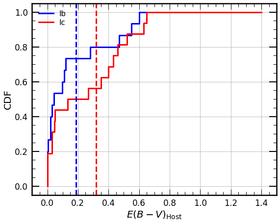
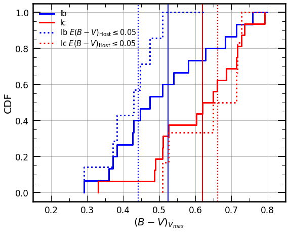
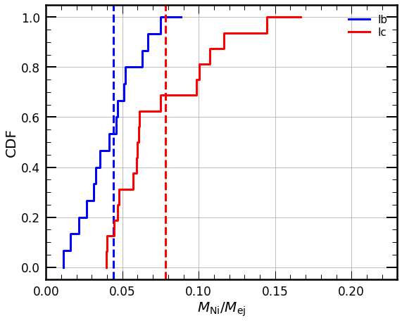
Figure 1: Top panel: Cumulative distribution of $E(B-V)_{\mathrm{Host}}$ (top), the $B-V$ color at the $V$-band peak after the host extinction correction (middle), $M_{\mathrm{Ni}}/M_{\mathrm{ej}}$ (bottom) of our SN Ib/Ic sample. The dotted line in the middle panel is the cumulative distribution of $(B-V)_{V_{\mathrm{max}}}$ for the case of minimal reddening (i.e., $E(B-V)_{\mathrm{Host}}\leq 0.05$). The vertical lines indicate the mean value of each distribution. See the text for more details.

The majority of our sample SN Ib/Ic photometric data are collected from the Open Supernova Catalog (OSC) (Guillochon et al., 2017). SNe Ib/Ic that have more than 30 photometric data points are selected. We exclude superluminous SNe Ic, broad-lined SNe Ic, and Ca-rich SNe Ib to focus our discussion on ordinary SNe Ib/Ic. Then SNe Ib/Ic that have the main peak information in the $V$-band and have more than three $B$-band and $V$-band data points within $\pm 5$ days with respect to the $V$-band peak epoch are selected to obtain a reasonably good $B-V$ color estimate at the $V$-band peak.

The host galaxy extinction for SNe Ib/Ic is usually non-negligible due to their dusty environments. In Table 1, we present the host extinction value of $E(B-V)_{\mathrm{Host}}$ extracted from the literature and the corresponding method to determine it for each SN in the 7th and 8th columns respectively, along with the references in the 9th column where details on the host extinction estimates can be found. The host extinction for SN 1999ex was obtained from the light curves of the Type Ia SN 1999ee, which occurred in the same host galaxy, assuming that it is not much different from that of SN 1999ee (Stritzinger et al., 2002). For SN 2004dn, Drout et al. (2011) use the small scatter in the $V-R$ color of SN Ib/Ic at 10 days after the $V$-band peak and the Galactic extinction law to obtain the host extinction. For the rest of the sample, either the ‘NaID’ or ‘Template’ method was used as indicated in the table. Here, the NaID method denotes the conventional way of using the equivalent width of Na I D absorption lines (e.g., Munari & Zwitter, 1997; Poznanski et al., 2012). The ‘Template’ method means the new method introduced by Stritzinger et al. (2018). These authors constructed a post-maximum color template for each subtype of SESNe (i.e., SN IIb, Ib and Ic) from the optical and near-infrared light curves of 3 minimally reddened SNe of each subtype and use them to infer the host extinctions of other SNe.

In the top panel of Figure 1, cumulative distributions of $E(B-V)_{\mathrm{Host}}$ are presented for both SNe Ib and Ic. The overall host extinction is larger for SNe Ic ($\overline{E(B-V)}_{\mathrm{Host}}$= 0.32) than for SNe Ib ($\overline{E(B-V)}_{\mathrm{Host}}$= 0.19). This implies different progenitor environments for SNe Ib and Ic: SNe Ic seem to originate from more dusty environments than SNe Ib, where more active star formation is expected.

Corrected for both the foreground extinction and the host galaxy extinction, the $B-V$ color at the $V-$band peak, $(B-V)_{\mathrm{Vmax}}$, is obtained and the corresponding cumulative distribution is presented in the middle panel of Figure 1 with the solid lines. It is observed that SNe Ib are systematically bluer ($\overline{(B-V)}_{\mathrm{Vmax}}$= 0.52) than SNe Ic ($\overline{(B-V)}_{\mathrm{Vmax}}$= 0.62), with an average color difference of $\Delta\overline{(B-V)}_{\mathrm{Vmax}}$ = 0.10 despite the fact that systematically larger extinction corrections are applied to SNe Ic than SNe Ib. The caveat is that there exist great uncertainties in the host extinction estimate. Munari & Zwitter (1997) show that the NaID method is less reliable for $E(B-V)\gtrsim 0.15$ because the Na I D lines are saturated. There are also multiple sources of uncertainties in this method, including possible diverse dust properties of SN host galaxies and the effects of the spectral resolution (e.g., Poznanski et al., 2011). The post-maximum color templates by Stritzinger et al. (2018) are based on a sample of small size (3 for each subtype) and the applicability of these templates needs to be further investigated with a larger sample of minimally reddened SESNe. For this reason we also present the cumulative distributions of $\overline{(B-V)}_{\mathrm{Vmax}}$ only for SNe Ib/Ic having a very small extinction(i.e., $E(B-V)_{\mathrm{host}}\leq 0.05$) with the dotted lines (8 SNe Ib and 7 SNe Ic). With this minimally reddened sample, the systematic color difference between SNe Ib and Ic becomes even more significant (i.e., $\Delta\overline{(B-V)}_{\mathrm{Vmax}}$= 0.22). We conclude that this color difference probably reflects intrinsic properties of SNe Ib/Ic.

The inferred values of $M_{\mathrm{Ni}}$ and $M_{\mathrm{ej}}$ of the same SNe are also collected from the literature as indicated in Table 1, and their ratios are presented in the bottom panel of Figure 1. SNe Ic have a systematically higher ⁵⁶Ni mass to ejecta mass ratio ($\overline{M_{\mathrm{Ni}}/M_{\mathrm{ej}}}$= 0.08) than SNe Ib ($\overline{M_{\mathrm{Ni}}/M_{\mathrm{ej}}}$= 0.04). As discussed below, a higher $M_{\mathrm{Ni}}/M_{\mathrm{ej}}$ would lead to a bluer color for a given SN ejecta property, meaning that the systematic redder color of SNe Ic than SNe Ib could not be attributed to different $M_{\mathrm{Ni}}/M_{\mathrm{ej}}$ ratios. The caveat is that we find great uncertainties in the estimates of $M_{\mathrm{Ni}}$ and $M_{\mathrm{ej}}$ in the literature. For example, in the case of SN 2007C, we get $M_{\mathrm{Ni}}=0.18~{}M_{\odot}$ & $M_{\mathrm{ej}}=1.83~{}M_{\odot}$ in Cano (2013) and $M_{\mathrm{Ni}}=0.07M_{\odot}$ & $M_{\mathrm{ej}}=6.2~{}M_{\odot}$ in Taddia et al. (2018). In the discussion below, therefore, we do not try to reproduce observed light curves of individual SNe but focus on general features of our models and qualitative comparison with the observation.

3 Supernova models

3.1 Methods and physical assumptions

We construct SN models from helium-rich and helium-poor progenitors for various $M_{\mathrm{ej}}$, different amounts of ⁵⁶Ni, and different ⁵⁶Ni distributions in the SN ejecta to explore the effects of these factors on the $B-V$ color.

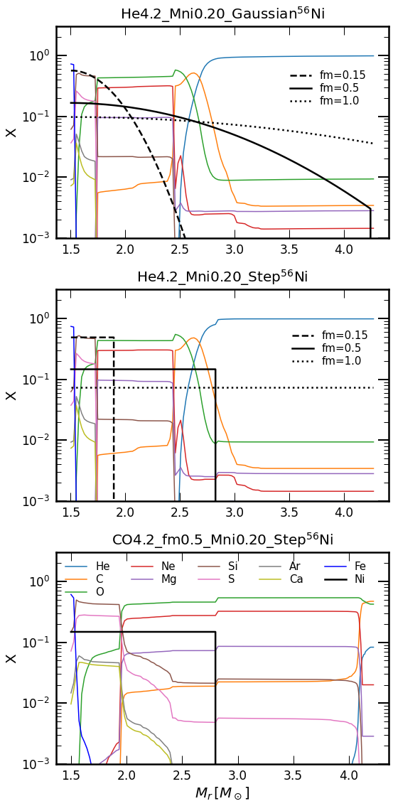
Figure 2: Mass fractions of different chemical elements in the He4.2 model with Gaussian ⁵⁶Ni distributions (top), with step ⁵⁶Ni distributions (middle), and in the CO4.2 model with a step ⁵⁶Ni distribution (bottom).

Table 2: Progenitor model properties

Name	$M_{\mathrm{ej}}$	$R$	$M_{\mathrm{CO}}$	$Y_{\mathrm{s}}$	$m_{\mathrm{He}}$	$M_{\mathrm{Fe}}$	$M_{\mathrm{ext}}$	Name	$M_{\mathrm{ej}}$	$R$	$M_{\mathrm{CO}}$	$Y_{\mathrm{s}}$	$m_{\mathrm{He}}$	$M_{\mathrm{Fe}}$	$M_{\mathrm{ext}}$
	[$M_{\odot}$]	[$R_{\odot}$]	[$M_{\odot}$]		[$M_{\odot}$]	[$M_{\odot}$]	[$M_{\odot}$]		[$M_{\odot}$]	[$R_{\odot}$]	[$M_{\odot}$]		[$M_{\odot}$]	[$M_{\odot}$]	[$M_{\odot}$]
He3.1	1.73	31.66	1.56	0.98	1.43	1.30	0.018	CO3.2	1.77	0.20	3.18	0.12	0.04	1.39	0.018
He3.5	2.06	4.77	2.02	0.98	1.44	1.41	0.022	CO3.6	2.05	0.21	3.61	0.12	0.07	1.53	0.021
He3.9	2.40	6.73	2.17	0.98	1.66	1.44	0.024	CO3.9	2.49	0.77	3.92	0.49	0.10	1.41	0.024
He4.2	2.76	2.45	2.63	0.98	1.58	1.45	0.027	CO4.2	2.72	0.22	4.19	0.08	0.06	1.45	0.027
He5.3	3.75	0.87	3.95	0.82	0.63	1.50	0.038	CO5.3	3.76	0.59	5.13	0.30	0.22	1.46	0.038
He5.6	4.10	1.62	3.64	0.98	1.62	1.48	0.041	CO5.7	4.08	0.20	5.56	0.30	0.17	1.63	0.041

We still do not fully understand evolutionary paths of massive stars towards SNe Ib or Ic and their mass-loss history (see Yoon, 2017, for a detailed discussion). In this study, we do not aim to investigate pre-SN evolution but instead consider diverse physical properties of SN Ib/Ic progenitors at the pre-SN stage to investigate their impact on the supernova light curves and colors. For this purpose, we adopt different mass-loss rates from helium stars to construct both helium-rich and helium-poor models having various final masses as explained below. All the progenitor models have the solar metallicity (i.e., $Z=0.02$) and are evolved until the infall velocity of the iron core exceeds 1000 $\mathrm{km~{}s^{-1}}$ using the MESA code (Paxton et al., 2011, 2013, 2015, 2018, 2019).

The helium-rich progenitor models contain more than 0.6$M_{\odot}$ of helium (He models) and the helium-poor progenitor models contain less than 0.2$M_{\odot}$ of helium (CO models). Each progenitor model is named to indicate their progenitor type and total mass. E.g., He3.1 refers to a helium-rich progenitor with its total mass of 3.1 $M_{\odot}$. We use the same notation when referring to the SN model from the respective progenitor model. See Table 2 for the details on the progenitor properties.

He3.1 and He3.9 are taken from the binary models Sm11p200d and Sm15p50 of Yoon et al. (2017), respectively. He3.5, He4.2 and He5.6 are obtained by evolving pure helium star models having initial masses of 4.0, 5.0, and 7.0 $M_{\odot}$ using the Wolf-Rayet mass-loss rate prescription by Nugis & Lamers (2000). He5.3 is obtained by evolving a 9.0 $M_{\odot}$ helium star with the Wolf-Rayet mass-loss rate prescription by Yoon (2017). CO3.2, CO3.6 and CO4.2 are obtained by evolving 7.0, 8.0, and 10.0 $M_{\odot}$ helium stars with the Yoon mass-loss prescription until core helium exhaustion, and with an artificially enhanced mass-loss rate (i.e., 500 times the standard Nugis & Lamers rate) thereafter until core-collapse. CO3.9 and CO5.9 models are constructed in a similar fashion by evolving 7.0 and 10.0 $M_{\odot}$ helium stars but the Nugis & Lamers mass-loss prescription is used during the core-helium burning phase. CO5.3 is calculated with a 11.0 $M_{\odot}$ helium star model using the Yoon mass-loss prescription throughout the whole evolution. Some example MESA inlist files for constructing these progenitor models can be found at ZENODO: https://doi.org/10.5281/zenodo.7797106 (catalog 10.5281/zenodo.7797106).

The final masses span $M_{\mathrm{tot}}=3.1\cdots 5.7M_{\odot}$, and the corresponding ejecta masses span $M_{\mathrm{ej}}=1.7\cdots 4.1M_{\odot}$ with the assumption of this study that the mass cut in SN explosion is located at the outer boundary of the iron core. This range encompasses a large fraction of the inferred ejecta masses of $M_{\mathrm{ej}}\approx 1.0\cdots 5.0M_{\odot}$ of SNe Ib/Ic (e.g., Drout et al., 2011; Cano, 2013; Lyman et al., 2016; Taddia et al., 2018; Zheng et al., 2022). An external material having a mass of about $1\%$ of the ejecta mass and an extent of $10^{14}$cm is attached to each progenitor model to avoid acceleration of the forward shock to a relativistic velocity because the relativistic effects cannot be properly handled in the version of the STELLA code that is used for this study (see Yoon et al., 2019, for more disucssion on this.). This external matter does not affect the light curve after about one day from the shock breakout, thus not affecting our focus of the study.

We use the STELLA code that is a one-dimensional multi-group radiative-hydrodynamics code for calculating SN light curves in multi-bands. The SN explosion is simulated by a thermal bomb at the mass cut, and time-dependent radiative transfer equations and hydrodynamics equations are solved simultaneously for approximately 100 frequency bins. For more detailed information, see Blinnikov & Tolstov (2011). See also Yoon et al. (2019) for a recent example of SNe Ib/Ic models calculated with the STELLA code.

We consider two kinetic energies, four ⁵⁶Ni masses, and six ⁵⁶Ni distributions to construct SN models for a given progenitor model. Kinetic energies of 1B and 2B are obtained by adjusting the explosion energy. We do not calculate explosive nucleosynthesis but instead radioactive ⁵⁶Ni is artificially introduced into the ejecta as in Yoon et al. (2019). The considered ⁵⁶Ni masses are $M_{\mathrm{Ni}}$=0.07$M_{\odot}$, 0.14$M_{\odot}$, 0.20$M_{\odot}$, and 0.25$M_{\odot}$. These sets of kinetic energies and ⁵⁶Ni masses cover most of the observed values of ordinary SNe Ib/Ic (e.g., Drout et al., 2011; Cano, 2013; Lyman et al., 2016; Taddia et al., 2018; Zheng et al., 2022).

The ⁵⁶Ni mass fraction in the SN ejecta is set to follow either a step distribution or a Gaussian distribution. For a step distribution, we adopt $X_{\textrm{Ni}}(M_{r})=\frac{M_{\textrm{Ni}}}{f_{\textrm{m}}(M_{\textrm{tot}}-M_{\textrm{cut}})}$ for $M_{\textrm{cut}}<M_{r}<f_{\textrm{m}}(M_{\textrm{tot}}-M_{\textrm{cut}})+M_{\textrm{cut}}$ and $X_{\textrm{Ni}}(M_{r})=0$ elsewhere. Here, $M_{r}$ is the mass coordinate, $M_{\textrm{cut}}$ the mass cut which corresponds to the outer boundary of the iron core, $M_{\textrm{tot}}$ the total mass of the progenitor, and $f_{\textrm{m}}$ is a free parameter that controls the shape of the ⁵⁶Ni distribution in the ejecta. For a Gaussian distribution, we adopt $X_{\textrm{Ni}}(M_{r})=A\textrm{exp}\left(-\left[\frac{M_{r}-M_{\textrm{cut}}}{f_{\textrm{m}}(M_{\textrm{tot}}-M_{\textrm{cut}})}\right]^{2}\right)$ where $A$ is the normalization factor. In the study, $f_{\textrm{m}}$=0.15, 0.5, and 1.0 are considered for both step and Gaussian ⁵⁶Ni distributions to account for the uncertainty in ⁵⁶Ni mixing. The value of $f_{\textrm{m}}$=0.15 ($f_{\textrm{m}}$=0.5) corresponds to a weak (moderate) ⁵⁶Ni mixing. The value of $f_{\textrm{m}}$=1.0 means complete or almost full ⁵⁶Ni mixing for the step and Gaussian distributions, respectively. In Figure 2, we present chemical profiles in the ejecta of He4.2 and CO4.2 models for various ⁵⁶Ni distributions, as an example. Note that the gamma-ray transfer in STELLA is treated in one-group approximation calibrated against full Monte-Carlo transport and, in principle, the deposition of the gamma-ray energy may take place far away from the birthplace of gamma photons in ⁵⁶Ni and ⁵⁶Co decays. In practice this non-local heating occurs only at late phases when the mean free path of gamma photons becomes large due to low density. In this study, however, we focus on relatively early phases where the mean free path of gamma photons is short and the heating is effectively local.

3.2 Model color distributions

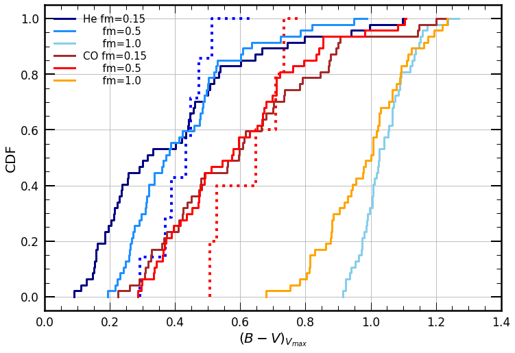
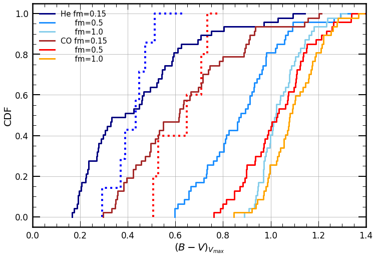
Figure 3: Upper panel: Cumulative distributions of $(B-V)_{\mathrm{Vmax}}$ of the STELLA models with the step ⁵⁶Ni distributions. The observed distributions of our minimally reddened (i.e., $E(B-V)_{\mathrm{host}}\leq 0.05$) SN Ib and Ic sample are given by the dotted blue and red lines. The average value of each case is given in Table 3. Lower Panel: Same as in the upper panel, but for the Gaussian ⁵⁶Ni distributions.

Table 3: Average $(B-V)_{\mathrm{Vmax}}$ values

$f_{\mathrm{m}}$	Step		Gauss
	He	CO	He	CO
0.15	0.40	0.61	0.45	0.65
0.5	0.43	0.59	0.88	1.04
1.0	1.04	0.99	1.05	1.10

The cumulative distributions of $(B-V)_{\mathrm{Vmax}}$ predicted by the models are presented in Figures 3 for both step and Gaussian ⁵⁶Ni distributions. Although the SN parameters (i.e., $E_{\mathrm{K}}$, $M_{\mathrm{ej}}$ and $M_{\mathrm{Ni}}$) of our models are chosen to reproduce ordinary SNe Ib/Ic, a precise quantitative comparison of the predicted $(B-V)_{\mathrm{Vmax}}$ with the observation would require a proper consideration of the exact distributions of these parameters within the selected SN Ib/Ic observation sample. However, there exist great uncertainties in the observationally inferred values of these parameters as discussed above and we limit our discussion to a qualitative comparison between the model prediction and the observed values of $(B-V)_{\mathrm{Vmax}}$.

The He models with the step ⁵⁶Ni distributions have a bluer color ($\overline{(B-V)}_{\mathrm{Vmax}}=0.40-0.43$) than the CO models ($\overline{(B-V)}_{\mathrm{Vmax}}\sim 0.60$), except for the fully mixed case ($f_{\mathrm{m}}$=1.0) that leads to $\overline{(B-V)}_{\mathrm{Vmax}}\simeq 1.0$ for both He and CO models. The systematic color difference between He and CO models is $\Delta\overline{(B-V)}_{\mathrm{Vmax}}\approx$ 0.21 (0.16) for $f_{\mathrm{m}}$=0.15 ($f_{\mathrm{m}}$=0.5), which is comparable to the observed color difference between SNe Ib and Ic (i.e., $\Delta\overline{(B-V)}_{\mathrm{Vmax}}=$ 0.10 and 0.22 for the full and minimally reddened samples, respectively).

The He models with the Gaussian ⁵⁶Ni distributions also have a bluer color ($\overline{(B-V)}_{\mathrm{Vmax}}\approx$ 0.45 & 0.88) than CO models ($\overline{(B-V)}_{\mathrm{Vmax}}\approx$ 0.65 & 1.04) when ⁵⁶Ni is not fully mixed ($f_{\mathrm{m}}$=0.15 & 0.5), and the differences between them are $\Delta\overline{(B-V)}_{\mathrm{Vmax}}\approx$ 0.20 and 0.16, which are also comparable to the observed color difference. Compared to the models with the step ⁵⁶Ni distributions, the models with Gaussian ⁵⁶Ni distributions were systematically redder for a given $f_{\mathrm{m}}$. The difference is most prominent when $f_{\mathrm{m}}$=0.5, showing the color difference of $\Delta\overline{(B-V)}_{\mathrm{Vmax}}\approx$ 0.45 between the step and the Gaussian ⁵⁶Ni distributions. This is because the ⁵⁶Ni abundance in the outer layer of the ejecta is higher in the models with a Gaussian distribution for a given $f_{\mathrm{m}}$ value. See Section 4.3 for a detailed discussion on the effect of mixing. On the other hand, the results with $f_{\mathrm{m}}=1.0$ are similar to the case of the step ⁵⁶Ni distributions because ⁵⁶Ni is fully mixed throughout the ejecta for both cases.

4 Possible origins of the color difference between SNe Ib and Ic

According to our models, there could be three possible reasons for the systematic difference in the observed $(B-V)_{\mathrm{Vmax}}$ values of SNe Ib and Ic.

• Different $M_{\mathrm{Ni}}/M_{\mathrm{ej}}$ ratios between SNe Ib and Ic.

• Different amounts of helium in the SNe Ib/Ic progenitors.

• Different degrees of ⁵⁶Ni mixing in the SNe Ib/Ic ejecta.

Here we discuss each possibility in detail.

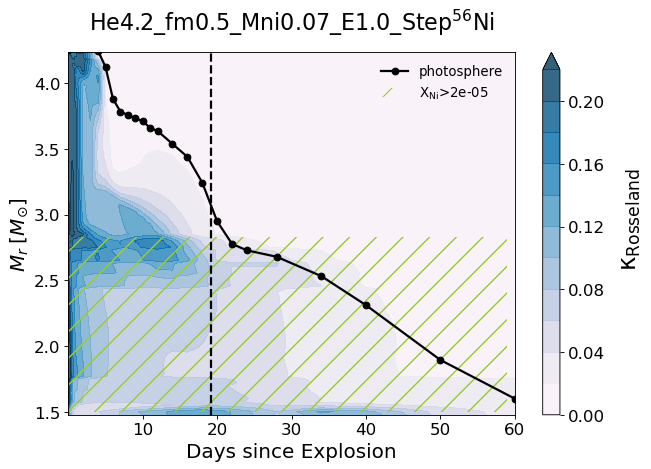
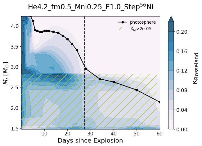
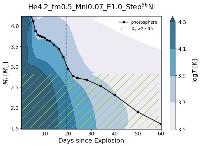
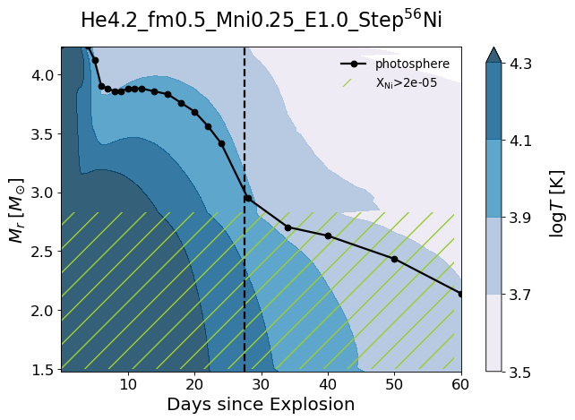
Figure 4: The Rosseland-mean opacity evolution and the gas temperature evolution of the models for two different ⁵⁶Ni mass: $M_{\textrm{Ni}}$=0.07$M_{\odot}$ (left panels) and 0.25$M_{\odot}$ (right panels). The models have a step ⁵⁶Ni distribution. The vertical dashed line represents the $V-$band peak epoch.

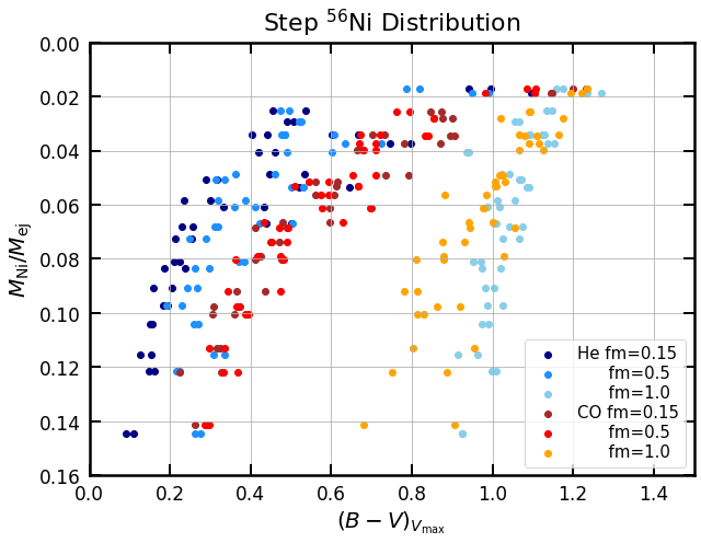
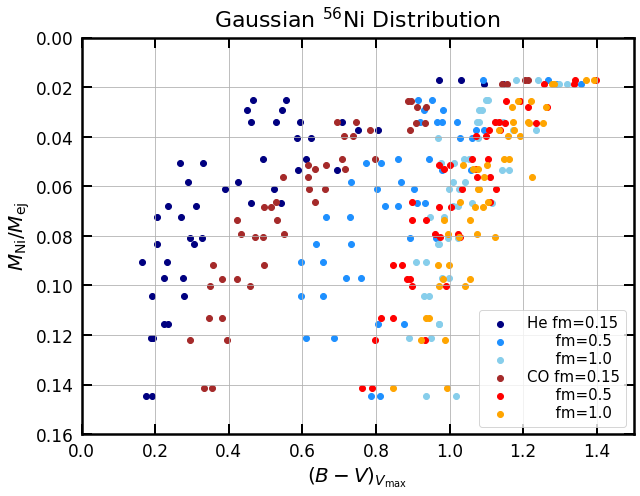
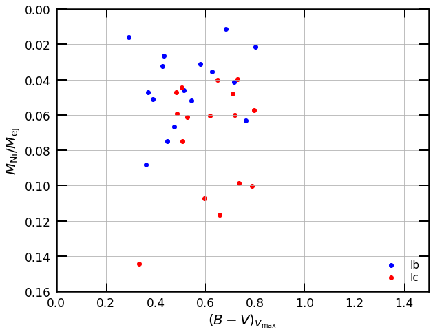
Figure 5: The dependency of $(B-V)_{\mathrm{Vmax}}$ on $M_{\textrm{Ni}}/M_{\textrm{ej}}$. The SN models with the step (top panel) and Gaussian (middle panel) ⁵⁶Ni distributions are the same models which are presented in Figure 3. The data from our SN Ib/Ic sample are also presented (bottom). Mind that the y-axis is flipped.

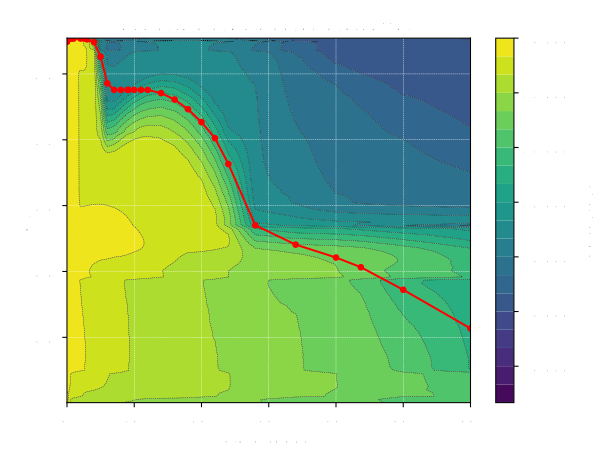
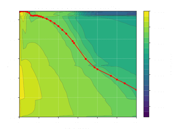
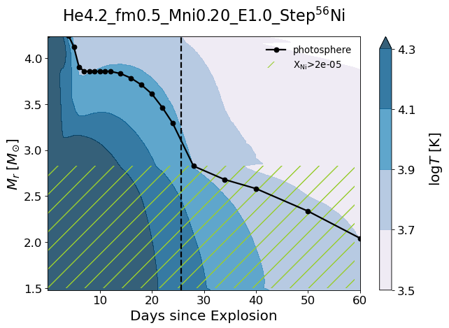
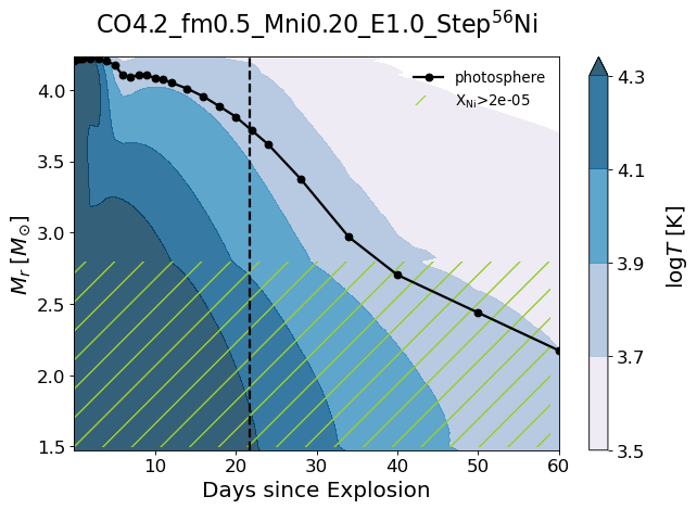
Figure 6: The evolution of the electron to baryon number density and the gas temperature evolution of the models with different chemical structures. The models have step ⁵⁶Ni distribution. Left panels correspond to a He model, right panels correspond to a CO model. Vertical dashed line represents the $V-$band peak epoch.

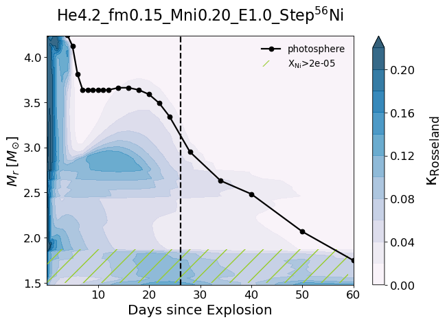
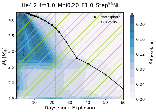
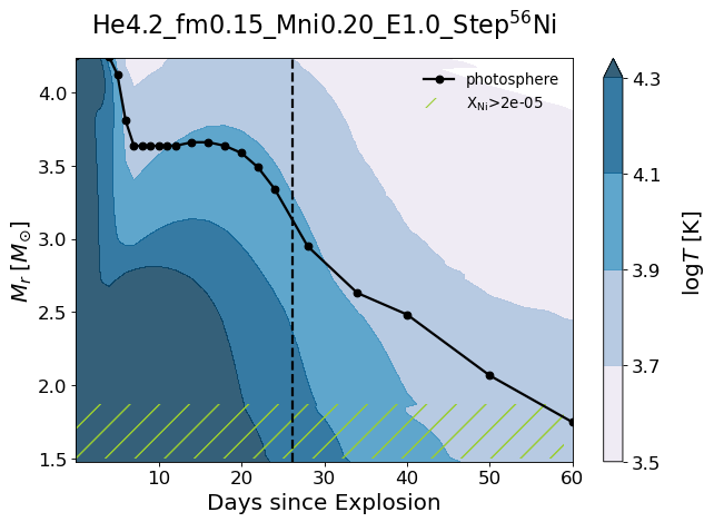
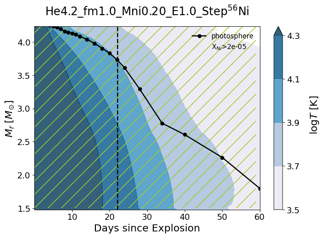
Figure 7: The Rosseland-mean opacity evolution and the gas temperature evolution of the models with different degrees of ⁵⁶Ni mixing. The models have step ⁵⁶Ni distribution. Left panels correspond to $f_{\mathrm{m}}$=0.15, right panels correspond to $f_{\mathrm{m}}$=1.0. Vertical dashed line represents the $V-$band peak epoch.

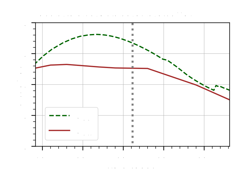
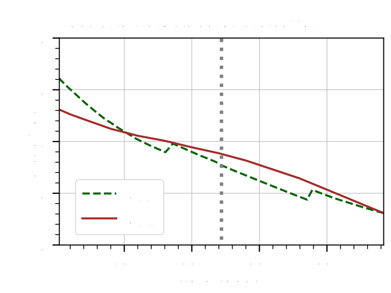
Figure 8: Evolution of the effective temperature ($T_{\mathrm{eff}}$; solid line) at the photosphere determined by the Rosseland-mean opacity and the temperature from the black-body fit to the SN spectrum ($T_{\mathrm{bb}}$; dashed line) in the He4.2 models with $M_{\mathrm{Ni}}=0.20M_{\odot}$ and $E_{\mathrm{K}}=1.0$ B for two different step ⁵⁶Ni distributions of $f_{\mathrm{m}}=0.15$ (left panel) and $f_{\mathrm{m}}=1.0$ (right panel). The vertical dotted line marks the epoch when the $V-$band peak is reached.

4.1 Ratio of ⁵⁶Ni mass to ejecta mass

SN ejecta with more ⁵⁶Ni for given ejecta mass and explosion energy would have a larger thermal energy due to the extra heating. Figure 4 compares the evolution of the Rosseland-mean opacity and gas temperature in the ejecta of the He4.2 model with $f_{\mathrm{m}}=0.5$ for two different ⁵⁶Ni masses, $M_{\mathrm{Ni}}$=0.07$M_{\odot}$ and 0.25$M_{\odot}$. The ejecta with $M_{\mathrm{Ni}}$=0.25$M_{\odot}$ is hotter at every mass zone for a given epoch compared to the case of $M_{\mathrm{Ni}}$=0.07$M_{\odot}$. Accordingly, the ejecta is more opaque because of more free electrons in the outer layers of the ejecta, and the photosphere retreats more slowly. The photospheric gas temperature remains in between $3.9<\log T[\mathrm{K}]<4.1$ at $t=8-29$ d. When the $V$-band peak appears at $t=27.5$ d, the effective temperature at the Rosseland-mean photosphere ($T_{\mathrm{eff}}$) and the black-body fit temperature of the SN spectrum ($T_{\mathrm{bb}}$), which is more relevant to the SN color than the effective temperature, are $T_{\mathrm{eff}}=7820$ K and $T_{\mathrm{bb}}=8320$ K, respectively. The corresponding $B-V$ is $(B-V)_{\mathrm{Vmax}}=0.22$. On the other hand, The photospheric temperature of the $M_{\mathrm{Ni}}=0.07M_{\odot}$ model stays in $3.9<\log T[\mathrm{K}]<4.1$ at $t=11-19$ d, duration of which is shorter than the $M_{\mathrm{Ni}}=0.25M_{\odot}$ case. At the $V$-band peak ($t=19.2$ d), the effective and black-body fit temperatures are $T_{\mathrm{eff}}=7370$ K and $T_{\mathrm{bb}}=7240$ K, respectively. The corresponding $B-V$ is $(B-V)_{\mathrm{Vmax}}=0.47$. This comparison illustrates that a higher $M_{\mathrm{Ni}}$ to $M_{\mathrm{ej}}$ ratio leads to a bluer optical color at the $V$-band peak for a given initial condition.

The dependency of $(B-V)_{\mathrm{Vmax}}$ on $M_{\textrm{Ni}}/M_{\textrm{ej}}$ can also be observed in Figure 5. As $M_{\textrm{Ni}}/M_{\textrm{ej}}$ becomes larger, $(B-V)_{\mathrm{Vmax}}$ of the models tends to decrease for a given ⁵⁶Ni distribution (note that the $y$-axis in the figure is flipped). By comparing the model color distributions presented in Figures 3 with the top and middle panels of Figure 5, we can find that the spread of $(B-V)_{\mathrm{Vmax}}$ for a given progenitor model and ⁵⁶Ni distribution mainly originates from the $M_{\textrm{Ni}}/M_{\textrm{ej}}$ spread. For example, the $(B-V)_{\mathrm{Vmax}}$ distribution of the CO models with a step ⁵⁶Ni distribution of $f_{\mathrm{m}}$=0.5 has the red end of the color distribution ($(B-V)_{\mathrm{Vmax}}$=1.1) when the models have the smallest $M_{\textrm{Ni}}/M_{\textrm{ej}}$=0.02 and the blue end of the color distribution ($(B-V)_{\mathrm{Vmax}}$=0.3) when the models have the largest $M_{\textrm{Ni}}/M_{\textrm{ej}}$=0.14.

It seems that the observed SN Ib/Ic sample does not follow the relation between $M_{\textrm{Ni}}/M_{\textrm{ej}}$ and $(B-V)_{\mathrm{Vmax}}$ predicted by the STELLA models (see the bottom panel of Figure 5). This might be due to the limited sample size, the lack of ⁵⁶Ni mixing information, poor estimates of ejecta/explosion parameters, or host extinctions. Future extensive investigation into SNe Ib/Ic photometry would test the validity of our model prediction.

If $M_{\mathrm{Ni}}/M_{\mathrm{ej}}$ were systematically larger in SNe Ib than SNe Ic, it could explain the systematic bluer color of SNe Ib than SNe Ic of our SN sample (the middle panel of Figure 1). In contrast to this expectation, however, it seems that SNe Ic have systematically larger $M_{\mathrm{Ni}}/M_{\mathrm{ej}}$ than SNe Ib in our SN sample (the bottom panel of Figure 1). The same trend is also found in the most recent dataset of SNe Ib/Ic provided by Zheng et al. (2022). We therefore conclude that the color difference between SNe Ib and Ic cannot be attributed to different $M_{\mathrm{Ni}}$ to $M_{\mathrm{ej}}$ ratios. However, given the large uncertainty in the estimates of $M_{\mathrm{Ni}}$ and $M_{\mathrm{ej}}$ as discussed in Section 2, this conclusion should be only considered tentative.

4.2 Helium contents in the progenitor

According to the most popular SN scenario, SNe Ib and Ic progenitors are helium-rich and helium-poor, respectively (e.g., Yoon, 2015). This scenario has been supported by many observational and theoretical studies as discussed in Section 1 (e.g., Matheson et al., 2001; Dessart et al., 2012; Hachinger et al., 2012; Liu et al., 2016; Fremling et al., 2018; Yoon et al., 2019; Dessart et al., 2020; Moriya et al., 2020; Teffs et al., 2020; Williamson et al., 2020; Shahbandeh et al., 2022). Recent stellar evolution models also suggest that SN Ib and Ic progenitors would not form a continuous sequence in terms of the He amount if mass-loss enhancement during the WC phase of WR stars, which is implied by recent WR star observations of the local universe, is assumed (see Yoon 2017 for detailed discussion and references therein; see also Woosley et al. 2021 and Aguilera-Dena et al. 2022). In this Section, we explore the consequence of the dichotomy nature of helium contents in the SN Ib/Ic color (see also Yoon et al., 2019).

In Figure 6, we present the evolution of the ratio of the free electron to baryon numbers ($n_{\mathrm{e}}/n_{\mathrm{b}}$) and the gas temperature in the ejecta of the He4.2 and CO4.2 models with $E_{\mathrm{K}}=1.0$ B, $M_{\mathrm{Ni}}=0.2~{}M_{\odot}$ and a step ⁵⁶Ni distribution ($f_{\mathrm{m}}=0.5$). In the He4.2 model, the ratio $n_{\mathrm{e}}/n_{\mathrm{b}}$ in the outermost layers (i.e., $M_{r}\gtrsim 4.0M_{\odot}$) rapidly decreases after $t\simeq 4$ d as the temperature decreases and the Rosseland-mean photosphere rapidly moves inwards accordingly in the mass-coordinate. However, in the CO4.2 model, more free electrons are available in the outer layers of the ejecta and the decrease of $n_{\mathrm{e}}/n_{\mathrm{b}}$ is relatively slow compared to the He4.2 model. This makes the photosphere of the CO4.2 model retreat inwards more slowly than in the He4.2 model: $M_{r,\mathrm{ph}}[M_{\odot}]=4.2\rightarrow 3.9\rightarrow 2.8$ (He4.2) and $M_{r,\mathrm{ph}}[M_{\odot}]=4.2\rightarrow 4.1\rightarrow 3.4$ (CO4.2) at $t=0$ d $\rightarrow$ 6 d $\rightarrow$ 28 d, respectively. The photospheric gas temperature at $t=5-28$ d is higher in He4.2 model ($3.9<\log T[\mathrm{K}]<4.1$) than in CO4.2 model ($3.7<\log T[\mathrm{K}]<3.9$).

The $V-$band peaks are reached when $t=25.6$ d and $t=21.8$ d for the He4.2 and CO4.2 models, and the corresponding effective and black-body fit temperatures are $T_{\mathrm{eff}}=7610$ K and $T_{\mathrm{bb}}=8234$ K for He4.2 and $T_{\mathrm{eff}}=6774$ K and $T_{\mathrm{bb}}=7327$ K for CO4.2, respectively.

For this reason, He models are systematically bluer than CO models for a given set of model parameters except for the (almost) full ⁵⁶Ni-mixing cases (i.e., $f_{\mathrm{m}}=1.0$; Figure 3). The effect of ⁵⁶Ni is discussed in the section that follows. As shown in Figure 3, the differences in $(B-V)_{\mathrm{Vmax}}$ between the two progenitor types (i.e., He and CO) in our models are $\Delta(B-V)_{\mathrm{Vmax}}\approx$ 0.14-0.18 for a given ⁵⁶Ni distribution, which is comparable to the $\Delta(B-V)_{\mathrm{Vmax}}$ value for our observation sample of SNe Ib/Ic. This is in good agreement with the notion that SNe Ib originate from helium-rich progenitors and SNe Ic from helium-poor progenitors.

4.3 ⁵⁶Ni mixing

Radioactive ⁵⁶Ni can significantly affect the SN color by radioactive heating, ionization induced by the heating, and line blanketing. Although a higher $M_{\mathrm{Ni}}/M_{\mathrm{ej}}$ leads to a bluer color at the optical peak for a given ⁵⁶Ni distribution as discussed in Section 4.1, we find that a stronger ⁵⁶Ni mixing can make the color redder at the $V$-band peak for a given $M_{\mathrm{Ni}}/M_{\mathrm{ej}}$ ratio, as shown in Figure 3: the fully mixed case ($f_{\mathrm{m}}$=1.0) results in a much redder color ($\overline{(B-V)}_{\mathrm{Vmax}}$ $\approx 1.0$) than weakly/moderately mixed cases ($f_{\mathrm{m}}$=0.15, 0.5, $\overline{(B-V)}_{\mathrm{Vmax}}$ $\approx 0.4-0.6$).

In Figure 7, we show the Rosseland-mean opacity and temperature evolution in the ejecta of the He4.2 models for $f_{\mathrm{m}}=0.15$ (weak ⁵⁶Ni mixing) and 1.0 (full ⁵⁶Ni mixing) with the step ⁵⁶Ni distributions. It is observed that in the case of $f_{\mathrm{m}}=0.15$, the ⁵⁶Ni heating of the outer layers is somewhat delayed, while the ejecta with $f_{\mathrm{m}}=1.0$ monotonically cools down given that ⁵⁶Ni is evenly distributed throughout the ejecta. Compared to the $f_{\mathrm{m}}$=1.0 case, the Rosseland-mean photosphere in the $f_{\mathrm{m}}$=0.15 model retreats more rapidly but stays in the hot ⁵⁶Ni-heated region ($\log T[\mathrm{K}]>3.9$ at $t=11-30$ d) during which the $V$-band peak appears at $t=26$ d. The Rosseland-mean photosphere in the $f_{\mathrm{m}}$=1.0 model recedes inwards more slowly and reaches the $V$-band peak earlier (i.e., at $t=22.1$ d). This is because of more free electrons in the outer layers due to the ⁵⁶Ni heating and line blanketing due to the presence of ⁵⁶Ni. This leads to lower effective and black-body fit temperatures for a stronger ⁵⁶Ni mixing at the $V$ band peak: $T_{\mathrm{eff}}=7528$ K and $T_{\mathrm{bb}}=83420$ K for $f_{\mathrm{m}}=0.15$ and $T_{\mathrm{eff}}=6760$ K and $T_{\mathrm{bb}}=6540$ K for $f_{\mathrm{m}}=1.0$.

The effect of line blanketing can also be observed by comparing the evolution of $T_{\mathrm{eff}}$ and $T_{\mathrm{bb}}$ as in Figure 8. In the case of $f_{\mathrm{m}}=0.15$, the Rosseland-mean photosphere remains in ⁵⁶Ni-free layers and $T_{\mathrm{bb}}$ is systematically higher than the effective temperature at the Rosseland-mean photosphere during the epochs around the $V-$band peak. This is because electron scattering causes the thermalisation depth to be located below the Rosseland-mean photosphere. The monochromatically scattered photons keep $T_{\mathrm{bb}}$ corresponding to those deep layers. Their number density is reduced by the dilution effect and the result is a bluer spectrum than the black-body spectrum corresponding to $T_{\mathrm{eff}}$. By contrast, $T_{\mathrm{bb}}$ is lower than $T_{\mathrm{eff}}$ in the $f_{\mathrm{m}}=1.0$ case because line blanketing due to ⁵⁶Ni obscures photons having short wavelengths and this is mainly responsible for the redder SN color with a stronger ⁵⁶Ni mixing.

We find that the colors of the Gaussian ⁵⁶Ni distribution models with weak and moderate ⁵⁶Ni mixing ($f_{\mathrm{m}}=$ 0.15 and 0.5) are systematically redder than the corresponding step ⁵⁶Ni distribution models (see Figure 3 and Table 3). This result can also be explained by the effects of ⁵⁶Ni on the SN spectral energy distribution. As seen in Figure 2, the ⁵⁶Ni distribution following the Gaussian function extends to the outermost layers even for the case of $f_{\mathrm{m}}=$ 0.15 and 0.5, while with the step function, ⁵⁶Ni is present only in the innermost confined region unless ⁵⁶Ni is fully mixed. Therefore, in the models with the Gaussian ⁵⁶Ni distribution, ⁵⁶Ni is always present at the Rosseland-mean photosphere and the resulting line blanketing makes the SN color redder than the corresponding step distribution models.

We conclude that different degrees of ⁵⁶Ni mixing would make the $(B-V)_{\mathrm{Vmax}}$ color different even when their progenitor types are the same in terms of helium content. However, it is not likely that the color difference between SNe Ib and Ic in our observation sample is soley due to this mixing effect.

Yoon et al. (2019) argue that the non-monotonic and monotonic color evolution observed in SNe Ib and some SNe Ic during early times implies relatively weak and very strong ⁵⁶Ni mixing in SN Ib and Ic ejecta, respectively. However, a stronger ⁵⁶Ni mixing into the helium-rich layer implies formation of strong He I lines during the photospheric phase (Dessart et al., 2012; Hachinger et al., 2012; Dessart et al., 2020; Teffs et al., 2020; Williamson et al., 2020). This means that if the redder color of SNe Ic compared to SNe Ib were mainly due to a stronger ⁵⁶Ni mixing, the SN Ic progenitors must be helium-poor. As shown in Section 4.2, on the other hand, helium deficiency would also lead to a redder color compared to the helium-rich case for a given ⁵⁶Ni distribution. Therefore, it is possible that, in reality, the redder color of SNe Ic compared to SNe Ib is related to both helium-deficiency and a stronger ⁵⁶Ni mixing.

5 Conclusions

We show that the optical colors of observed SNe Ib and SNe Ic are systematically different at the $V$-band peak in our selected sample (16 SNe Ib and 17 SNe Ic; Table 1): SNe Ib are bluer ($\overline{(B-V)}_{\mathrm{Vmax}}=0.52$) than SNe Ic ($\overline{(B-V)}_{\mathrm{Vmax}}=0.62$) by $\Delta\overline{(B-V)}_{\mathrm{Vmax}}=$ $0.10$, on average (Figure 1; Section 2). This color difference is found to be larger (i.e., $\Delta\overline{(B-V)}_{\mathrm{Vmax}}=0.22$) if we limit our sample to the minimally reddened case (i.e., $E(B-V)_{\mathrm{host}}\leq 0.05$).

Using multi-band radiation-hydrodynamics simulations with the STELLA code for both helium-rich and helium-poor progenitors of various final masses ($M\simeq 3.1\cdots 5.7M_{\odot}$), we explore three possible reasons for the color difference: 1) different $M_{\mathrm{Ni}}/M_{\mathrm{ej}}$ ratios (Section 4.1), 2) different amounts of helium (Section 4.2), and 3) different degrees of ⁵⁶Ni mixing in SN ejecta (Section 4.3). We find that the SN color becomes bluer at the $V-$band peak for a larger $M_{\mathrm{Ni}}/M_{\mathrm{ej}}$ ratio, a weaker ⁵⁶Ni mixing, and/or a helium-rich progenitor compared to the corresponding helium-poor case (Figure 3  and 5).

From these results, we draw the following conclusions:

1. In our sample of observed SNe, the $M_{\mathrm{Ni}}/M_{\mathrm{ej}}$ ratios in SNe Ic seem to be systematically higher than in SNe Ib (see Figure 1). This implies that if the inner structure and the degree of ⁵⁶Ni mixing in SNe Ib and SNe Ic were similar to each other, SNe Ic would be systematically bluer than SNe Ib, in sharp contrast to the observation. Therefore, we conclude that different $M_{\mathrm{Ni}}/M_{\mathrm{ej}}$ ratios cannot explain the color difference between SNe Ib and Ic (Section 4.1).

2. We also exclude the possibility that radioactive ⁵⁶Ni is almost fully mixed in both SNe Ib and SNe Ic ejecta, as otherwise no systematic $B-V$ color difference would be observed (see Figure 3).

3. We find that the $B-V$ color difference can be well explained by the standard scenario for SNe Ib and Ic (i.e., helium-rich and helium-poor progenitors for SNe Ib and SNe Ic, respectively), given that the color at the $V-$band peak is systematically redder with the helium-poor progenitors for a given ⁵⁶Ni distribution (unless ⁵⁶Ni is fully mixed). It is possible that the redder color of SNe Ic are partly due to a stronger ⁵⁶Ni mixing in the ejecta, compared to SNe Ib (Section 4.3). If this is the case, SNe Ic progenitors must be helium-poor as otherwise strong He I absorption lines would be detected in SN Ic spectra.

In short, we conclude that the systematic color difference between SNe Ib and SNe Ic at the $V-$band peak provides strong evidence for the distinct properties of their progenitors in terms of helium content, rebutting the existence of a large amount of hidden helium in SNe Ic.

This study is subject to a few limitations. First of all, STELLA might not predict broad-band colors at the optical peak accurately due to some physical simplifications implemented in the code, e.g., LTE approximation for atomic level populations, the limited number of spectral lines, the lack of proper treatment of the fluorescent effect, etc. Detailed spectrum calculations including these factors would be required for more rigorous and quantitative comparison of the models with the observation. Secondly, only a small number of SNe Ib/Ic (16/17 for each SN subtype) are used for the analysis because not many sufficiently good photometric or host extinction data are available. Future acquisition of large samples of SN Ib/Ic will allow us to confirm the results obtained in the study.

Finally, our model comparison with the observations is limited to the $B-V$ color at the optical peak. It would be interesting to extend our approach to post-maximum colors, which might provide further constraints on the nature of SNe Ib/Ic progenitors and the SN ejecta properties  (e.g., Drout et al., 2011; Dessart et al., 2015, 2016; Stritzinger et al., 2018; Woosley et al., 2021). However, the SN Ib/Ic colors during the post-maximum can be much more significantly affected by specific lines and non-LTE effects than earlier times (e.g., Dessart et al., 2015, 2016), which are not properly considered in the current version of STELLA. The time-dependent non-LTE effects are being implemented in STELLA and a more extended study on the SN Ib/Ic colors including post-maximum colors will be presented in the future.

Appendix A appendix section

Table 4: $M_{\mathrm{Ni}}$ and $M_{\mathrm{ej}}$ of our selected SN Ib/Ic sample

Name	$M_{\mathrm{Ni}}$ [$M_{\odot}$]	$M_{\mathrm{ej}}$ [$M_{\odot}$]
SN 1999ex	0.25 (R06), 0.1 (D11), 0.12 (C13), 0.15 (L16), 0.172 (P16)	0.9 (R06), 2.91 (C13), 2.9 (L16)
SN 2004gq	0.13 (D11), 0.14 (C13), 0.1 (L16), 0.11 (T18)	3.19 (C13), 1.8 (L16), 3.4 (T18)
SN 2004gv	0.14 (C13), 0.16 (T18)	11.72 (C13), 3.4 (T18)
SN 2006ep	0.06 (L16), 0.12 (T18)	2.7 (L16), 1.9 (T18)
SN 2006gi	0.064 (E11)	3.0 (E11)
SN 2006lc	0.3 (T15), 0.14 (T18)	3.67 (T15), 3.4 (T18)
SN 2007C	0.16 (D11), 0.18 (C13), 0.17 (L16), 0.07 (T18)	1.83 (C13), 1.9 (L16), 6.2 (T18)
SN 2007kj	0.066 (T18)	2.5 (T18)
SN 2007Y	0.03 (C13), 0.04 (L16), 0.051 (P16), 0.03 (T18)	2.09 (C13), 1.4 (L16), 1.9 (T18)
SN 2008D	0.07 (D11), 0.08 (C13), 0.09 (L16), 0.111 (P16)	5.33 (C13), 2.9 (L16)
SN 2009jf	0.18 (C13), 0.24 (L16), 0.271 (P16)	7.34 (C13), 4.7 (L16)
SN 2012au	0.3 (M13)	4.0 (M13)
SN 2014C	0.15 (M17)	1.7 (M17)
SN 2015ah	0.092 (P19)	2.0 (P19)
SN 2015ap	0.12 (P19)	1.8 (P19)
iPTF13bvn	0.06 (L16), 0.07 (P16)	1.7 (L16)
SN 1994I	0.08 (R06), 0.06 (D11), 0.06 (C13), 0.07 (L16), 0.102 (P16)	0.5 (R06), 0.72 (C13), 0.6 (L16)
SN 2004aw	0.27 (D11), 0.22 (C13), 0.2 (L16)	6.49 (C13), 3.3 (L16)
SN 2004dn	0.16 (D11), 0.15 (C13), 0.16 (L16)	3.4 (C13), 2.8 (L16)
SN 2004fe	0.19 (D11), 0.19 (C13), 0.23 (L16), 0.1 (T18)	2.07 (C13), 1.8 (L16), 2.5 (T18)
SN 2004gt	0.16 (T18)	3.4 (T18)
SN 2005aw	0.17 (T18)	4.3 (T18)
SN 2007gr	0.07 (D11), 0.04 (C13), 0.08 (L16), 0.073 (P16)	1.7 (C13), 1.8 (L16)
SN 2007hn	0.25 (T18)	1.5 (T18)
SN 2011bm	0.58 (C13), 0.62 (L16), 0.702 (P16)	18.75 (C13), 10.1 (L16)
SN 2013F	0.15 (P19)	1.4 (P19)
SN 2013ge	0.109 (P16)	2.5 (D16)
SN 2014L	0.075 (Z18)	1.0 (Z18)
SN 2016iae	0.13 (P19)	2.2 (P19)
SN 2016P	0.09 (P19)	1.5 (P19)
SN 2017ein	0.13 (X19)	0.9 (X19)
SN 2020oi	0.07 (R20)	0.71 (R20)
LSQ14efd	0.25 (J21)	2.49 (J21)

References

- Aguilera-Dena et al. (2022) Aguilera-Dena, D. R., Müller, B., Antoniadis, J., et al. 2022, arXiv e-prints, arXiv:2204.00025. https://arxiv.org/abs/2204.00025
- Barbarino et al. (2017) Barbarino, C., Botticella, M. T., Dall’Ora, M., et al. 2017, MNRAS, 471, 2463, doi: 10.1093/mnras/stx1709
- Barbarino et al. (2020) Barbarino, C., Sollerman, J., Taddia, F., et al. 2020, arXiv e-prints, arXiv:2010.08392. https://arxiv.org/abs/2010.08392
- Bianco et al. (2014) Bianco, F. B., Modjaz, M., Hicken, M., et al. 2014, ApJS, 213, 19, doi: 10.1088/0067-0049/213/2/19
- Blinnikov & Tolstov (2011) Blinnikov, S. I., & Tolstov, A. G. 2011, Astronomy Letters, 37, 194, doi: 10.1134/S1063773711010051
- Brown et al. (2014) Brown, P. J., Breeveld, A. A., Holland, S., Kuin, P., & Pritchard, T. 2014, Ap&SS, 354, 89, doi: 10.1007/s10509-014-2059-8
- Cano (2013) Cano, Z. 2013, MNRAS, 434, 1098, doi: 10.1093/mnras/stt1048
- Dessart et al. (2012) Dessart, L., Hillier, D. J., Li, C., & Woosley, S. 2012, MNRAS, 424, 2139, doi: 10.1111/j.1365-2966.2012.21374.x
- Dessart et al. (2011) Dessart, L., Hillier, D. J., Livne, E., et al. 2011, MNRAS, 414, 2985, doi: 10.1111/j.1365-2966.2011.18598.x
- Dessart et al. (2015) Dessart, L., Hillier, D. J., Woosley, S., et al. 2015, MNRAS, 453, 2189, doi: 10.1093/mnras/stv1747
- Dessart et al. (2016) —. 2016, MNRAS, 458, 1618, doi: 10.1093/mnras/stw418
- Dessart et al. (2020) Dessart, L., Yoon, S.-C., Aguilera-Dena, D. R., & Langer, N. 2020, A&A, 642, A106, doi: 10.1051/0004-6361/202038763
- Drout et al. (2011) Drout, M. R., Soderberg, A. M., Gal-Yam, A., et al. 2011, ApJ, 741, 97, doi: 10.1088/0004-637X/741/2/97
- Drout et al. (2016) Drout, M. R., Milisavljevic, D., Parrent, J., et al. 2016, ApJ, 821, 57, doi: 10.3847/0004-637X/821/1/57
- Elmhamdi et al. (2011) Elmhamdi, A., Tsvetkov, D., Danziger, I. J., & Kordi, A. 2011, ApJ, 731, 129, doi: 10.1088/0004-637X/731/2/129
- Folatelli et al. (2016) Folatelli, G., Van Dyk, S. D., Kuncarayakti, H., et al. 2016, ApJ, 825, L22, doi: 10.3847/2041-8205/825/2/L22
- Fremling et al. (2014) Fremling, C., Sollerman, J., Taddia, F., et al. 2014, A&A, 565, A114, doi: 10.1051/0004-6361/201423884
- Fremling et al. (2018) Fremling, C., Sollerman, J., Kasliwal, M. M., et al. 2018, A&A, 618, A37, doi: 10.1051/0004-6361/201731701
- Gal-Yam et al. (2005) Gal-Yam, A., Cenko, S. B., Fox, D. W., et al. 2005, in Astronomical Society of the Pacific Conference Series, Vol. 342, 1604-2004: Supernovae as Cosmological Lighthouses, ed. M. Turatto, S. Benetti, L. Zampieri, & W. Shea, 305. https://arxiv.org/abs/astro-ph/0410038
- Guillochon et al. (2017) Guillochon, J., Parrent, J., Kelley, L. Z., & Margutti, R. 2017, ApJ, 835, 64, doi: 10.3847/1538-4357/835/1/64
- Hachinger et al. (2012) Hachinger, S., Mazzali, P. A., Taubenberger, S., et al. 2012, MNRAS, 422, 70, doi: 10.1111/j.1365-2966.2012.20464.x
- Hunter et al. (2009) Hunter, D. J., Valenti, S., Kotak, R., et al. 2009, A&A, 508, 371, doi: 10.1051/0004-6361/200912896
- Jin et al. (2021) Jin, H., Yoon, S.-C., & Blinnikov, S. 2021, ApJ, 910, 68, doi: 10.3847/1538-4357/abe0b1
- Liu et al. (2016) Liu, Y.-Q., Modjaz, M., Bianco, F. B., & Graur, O. 2016, ApJ, 827, 90, doi: 10.3847/0004-637X/827/2/90
- Lucy (1991) Lucy, L. B. 1991, ApJ, 383, 308, doi: 10.1086/170787
- Lyman et al. (2016) Lyman, J. D., Bersier, D., James, P. A., et al. 2016, MNRAS, 457, 328, doi: 10.1093/mnras/stv2983
- Margutti et al. (2017) Margutti, R., Kamble, A., Milisavljevic, D., et al. 2017, ApJ, 835, 140, doi: 10.3847/1538-4357/835/2/140
- Matheson et al. (2001) Matheson, T., Filippenko, A. V., Li, W., Leonard, D. C., & Shields, J. C. 2001, AJ, 121, 1648, doi: 10.1086/319390
- Mazzali et al. (2008) Mazzali, P. A., Valenti, S., Della Valle, M., et al. 2008, Science, 321, 1185, doi: 10.1126/science.1158088
- Milisavljevic et al. (2013) Milisavljevic, D., Soderberg, A. M., Margutti, R., et al. 2013, ApJ, 770, L38, doi: 10.1088/2041-8205/770/2/L38
- Milisavljevic et al. (2015) Milisavljevic, D., Margutti, R., Kamble, A., et al. 2015, ApJ, 815, 120, doi: 10.1088/0004-637X/815/2/120
- Modjaz (2007) Modjaz, M. 2007, PhD thesis, Harvard University
- Modjaz et al. (2009) Modjaz, M., Li, W., Butler, N., et al. 2009, ApJ, 702, 226, doi: 10.1088/0004-637X/702/1/226
- Moriya et al. (2020) Moriya, T. J., Suzuki, A., Takiwaki, T., Pan, Y.-C., & Blinnikov, S. I. 2020, MNRAS, 497, 1619, doi: 10.1093/mnras/staa2060
- Munari & Zwitter (1997) Munari, U., & Zwitter, T. 1997, A&A, 318, 269
- Nugis & Lamers (2000) Nugis, T., & Lamers, H. J. G. L. M. 2000, A&A, 360, 227
- Oates et al. (2012) Oates, S. R., Bayless, A. J., Stritzinger, M. D., et al. 2012, MNRAS, 424, 1297, doi: 10.1111/j.1365-2966.2012.21311.x
- Paxton et al. (2011) Paxton, B., Bildsten, L., Dotter, A., et al. 2011, ApJS, 192, 3, doi: 10.1088/0067-0049/192/1/3
- Paxton et al. (2013) Paxton, B., Cantiello, M., Arras, P., et al. 2013, ApJS, 208, 4, doi: 10.1088/0067-0049/208/1/4
- Paxton et al. (2015) Paxton, B., Marchant, P., Schwab, J., et al. 2015, ApJS, 220, 15, doi: 10.1088/0067-0049/220/1/15
- Paxton et al. (2018) Paxton, B., Schwab, J., Bauer, E. B., et al. 2018, ApJS, 234, 34, doi: 10.3847/1538-4365/aaa5a8
- Paxton et al. (2019) Paxton, B., Smolec, R., Schwab, J., et al. 2019, ApJS, 243, 10, doi: 10.3847/1538-4365/ab2241
- Poznanski et al. (2011) Poznanski, D., Ganeshalingam, M., Silverman, J. M., & Filippenko, A. V. 2011, MNRAS, 415, L81, doi: 10.1111/j.1745-3933.2011.01084.x
- Poznanski et al. (2012) Poznanski, D., Prochaska, J. X., & Bloom, J. S. 2012, MNRAS, 426, 1465, doi: 10.1111/j.1365-2966.2012.21796.x
- Prentice et al. (2016) Prentice, S. J., Mazzali, P. A., Pian, E., et al. 2016, MNRAS, 458, 2973, doi: 10.1093/mnras/stw299
- Prentice et al. (2019) Prentice, S. J., Ashall, C., James, P. A., et al. 2019, MNRAS, 485, 1559, doi: 10.1093/mnras/sty3399
- Rho et al. (2021) Rho, J., Evans, A., Geballe, T. R., et al. 2021, ApJ, 908, 232, doi: 10.3847/1538-4357/abd850
- Richardson et al. (2006) Richardson, D., Branch, D., & Baron, E. 2006, AJ, 131, 2233, doi: 10.1086/500578
- Richmond et al. (1996) Richmond, M. W., van Dyk, S. D., Ho, W., et al. 1996, AJ, 111, 327, doi: 10.1086/117785
- Sahu et al. (2011) Sahu, D. K., Gurugubelli, U. K., Anupama, G. C., & Nomoto, K. 2011, MNRAS, 413, 2583, doi: 10.1111/j.1365-2966.2011.18326.x
- Shahbandeh et al. (2022) Shahbandeh, M., Hsiao, E. Y., Ashall, C., et al. 2022, ApJ, 925, 175, doi: 10.3847/1538-4357/ac4030
- Stritzinger et al. (2002) Stritzinger, M., Hamuy, M., Suntzeff, N. B., et al. 2002, AJ, 124, 2100, doi: 10.1086/342544
- Stritzinger et al. (2018) Stritzinger, M. D., Taddia, F., Burns, C. R., et al. 2018, A&A, 609, A135, doi: 10.1051/0004-6361/201730843
- Taddia et al. (2015) Taddia, F., Sollerman, J., Leloudas, G., et al. 2015, A&A, 574, A60, doi: 10.1051/0004-6361/201423915
- Taddia et al. (2018) Taddia, F., Stritzinger, M. D., Bersten, M., et al. 2018, A&A, 609, A136, doi: 10.1051/0004-6361/201730844
- Taubenberger et al. (2006) Taubenberger, S., Pastorello, A., Mazzali, P. A., et al. 2006, MNRAS, 371, 1459, doi: 10.1111/j.1365-2966.2006.10776.x
- Teffs et al. (2020) Teffs, J., Ertl, T., Mazzali, P., Hachinger, S., & Janka, H. T. 2020, MNRAS, 499, 730, doi: 10.1093/mnras/staa2549
- Tsvetkov & Bartunov (1993) Tsvetkov, D. Y., & Bartunov, O. S. 1993, Bulletin d’Information du Centre de Donnees Stellaires, 42, 17
- Valenti et al. (2011) Valenti, S., Fraser, M., Benetti, S., et al. 2011, MNRAS, 416, 3138, doi: 10.1111/j.1365-2966.2011.19262.x
- Valenti et al. (2012) Valenti, S., Taubenberger, S., Pastorello, A., et al. 2012, ApJ, 749, L28, doi: 10.1088/2041-8205/749/2/L28
- Van Dyk et al. (2018) Van Dyk, S. D., Zheng, W., Brink, T. G., et al. 2018, ApJ, 860, 90, doi: 10.3847/1538-4357/aac32c
- Williamson et al. (2020) Williamson, M., Kerzendorf, W., & Modjaz, M. 2020, arXiv e-prints, arXiv:2010.10528. https://arxiv.org/abs/2010.10528
- Woosley et al. (2021) Woosley, S. E., Sukhbold, T., & Kasen, D. N. 2021, ApJ, 913, 145, doi: 10.3847/1538-4357/abf3be
- Xiang et al. (2019) Xiang, D., Wang, X., Mo, J., et al. 2019, ApJ, 871, 176, doi: 10.3847/1538-4357/aaf8b0
- Yoon (2015) Yoon, S.-C. 2015, PASA, 32, e015, doi: 10.1017/pasa.2015.16
- Yoon (2017) —. 2017, MNRAS, 470, 3970, doi: 10.1093/mnras/stx1496
- Yoon et al. (2019) Yoon, S.-C., Chun, W., Tolstov, A., Blinnikov, S., & Dessart, L. 2019, ApJ, 872, 174, doi: 10.3847/1538-4357/ab0020
- Yoon et al. (2017) Yoon, S.-C., Dessart, L., & Clocchiatti, A. 2017, ApJ, 840, 10, doi: 10.3847/1538-4357/aa6afe
- Zhang et al. (2018) Zhang, J., Wang, X., Vinkó, J., et al. 2018, ApJ, 863, 109, doi: 10.3847/1538-4357/aaceaf
- Zheng et al. (2022) Zheng, W., Stahl, B. E., de Jaeger, T., et al. 2022, MNRAS, 512, 3195, doi: 10.1093/mnras/stac723