Vaccination compartmental epidemiological models for the delta and omicron SARS-CoV-2 variants

Abstract

We explore the inclusion of vaccination in compartmental epidemiological models concerning the delta and omicron variants of the SARS-CoV-2 virus that caused the COVID-19 pandemic. We expand on our earlier compartmental-model work by incorporating vaccinated populations. We present two classes of models that differ depending on the immunological properties of the variant. The first one is for the delta variant, where we do not follow the dynamics of the vaccinated individuals since infections of vaccinated individuals were rare. The second one for the far more contagious omicron variant incorporates the evolution of the infections within the vaccinated cohort. We explore comparisons with available data involving two possible classes of counts, fatalities and hospitalizations. We present our results for two regions, Andalusia and Switzerland (including the Principality of Liechtenstein), where the necessary data are available. In the majority of the considered cases, the models are found to yield good agreement with the data and have a reasonable predictive capability beyond their training window, rendering them potentially useful tools for the interpretation of the COVID-19 and further pandemic waves, and for the design of intervention strategies during these waves.

I Introduction

Over the last two and a half years, the COVID-19 pandemic has been deemed responsible, to date, for 760 million confirmed cases, and over 6.8 million deaths worldwide, as of this writing and according to the World Health Organization COVID-19 dashboard. As such, its emergence wreaked havoc in life as we knew it throughout the world and forced a dramatic modification of our social and economic activities during this interval. At the same time, it triggered a global mobilization of the scientific community to produce vaccines rapidly, especially through (thankfully, by that time, fairly mature) technology of mRNA-based methods. This effort led to the remarkable result of having a vaccine against SARS-CoV-2 within a year of its emergence. Nevertheless, this was far from the end of the story, as new variants of the SARS-CoV-2 virus kept emerging within 2020 and 2021. The so-called delta variant appeared in India in late 2020 and it had spread to 179 countries by November 2021. Subsequently, the delta variant was superseded by the so-called omicron variant that was reported in South Africa on November 2021, and subsequently became rapidly the predominant variant of SARS-CoV-2 thereafter.

The theoretical and mathematical modeling of infectious diseases such as COVID-19 has a long and time-honored history since the classic work of Kermack and McKendrick [1]. Moreover, relevant efforts have been summarized in numerous venues in recent years, such as, e.g., [2, 3, 4], to mention only a few. The urgency and severity of the COVID-19 pandemic brought about an intense effort on the side of the mathematical and physical communities to develop analytical models and computational tools that could be used to examine the unprecedented volume of available data regarding the temporal (and spatial) evolution of the pandemic and to make predictions for the weeks (or in some cases month(s)) ahead. A notable example of comparison of such efforts can be seen in, e.g., websites such as [5]. Relevant modeling efforts have now been summarized in a number of reviews such as [6, 7], including ones of specialized modeling aspects such as the study of metapopulation network models [8], while other works summarized the challenges and difficulties of associated modeling [9, 10].

Over the last year, a large portion of the focus of the modeling efforts has shifted towards the inclusion of vaccination in epidemniological models. While a lot of information is available regarding the effectiveness and efficacy of vaccines [11] (see also websites such as [12]) mathematical models can still be quite useful in a number of ways, including in guiding and informing distribution strategies thereof [13, 14]. It is in that light that numerous compartmental epidemiological models with vaccination strategies have arisen in the literature [15, 16], including some specific to different geographical locations [17] and to different social infrastructures, such as nursing homes [18]. While the relevant models feature different levels of complexity starting from SIRV (Susceptible-Infected-Recovered-Vaccinated) extensions of the classic SIR (Susceptible-Infected-Recovered) [15] model and progressively extending to multicomponent models such as, e.g., [19], our aim here is to build systematically on the earlier modeling attempt of [20] by considering SARS-CoV-2 variants that affect differently the vaccinated population.

More concretely, our aim is to present a model of the omicron variant (model A and its two implementations A1 and A2), in which its highly contagious nature allows for so-called breakthrough infections, whereby vaccinated individuals may still be infected. In that light, we account for the standard populations of our earlier work [20], including exposed, pre-symptomatics, and asymptomatics [21], as well as hospitalizations, recoveries and fatalities. In addition, we consider such populations in both the unvaccinated and vaccinated portions of the population and their interactions. The primary aim of the associated study is to explore the dynamical evolution of the omicron variant from the end of 2021 to early spring 2022. We also present a simpler model (model B) for the evolution of the earlier delta variant during the fall of 2021. In that case, vaccination was deemed to protect individuals from being infected, and the fraction of breakthrough infections was quite small, even in groups such as the potentially highly exposed group of healthcare workers [22]. Accordingly, we assume that the vaccinated population may be effectively removed from the susceptible compartment.

We examine two versions of the proposed omicron model in Section II (models A1 and A2), their difference motivated by data availability. The population flows in Model A1 terminate at the fatalities compartment: as such, the model considers that fatalities in both the unvaccinated and vaccinated populations provide the most reliable data. Model A2 is motivated by the existence of systematic data for the total number of hospitalizations (conventional and ICU): here, population flows terminate at the hospitalizations compartment, i.e., they do not branch further to the fatalities compartment as in model A1. This is for a number of reasons: in primis, reporting of fatalities occasionally occurs retroactively (and less reliably). Our models are applied to two regions with similar populations (approximately 8 million inhabitants): Andalusia and Switzerland (including the Principality of Liechtenstein) The motivation for this choice arises, once again, from the availability of suitably stratified data, whereby both fatalities and hospitalizations are available for vaccinated and unvaccinated individuals. In Section III we propose, in addition to the more detailed model for the omicron variant presented in Section II, a model for the delta variant, model B. We use model B in the same spatial regions. We typically find that numerical results compare favorably to available data, both in terms of the comparison of the regression results and also in connection to testing beyond the end of the training period for the model parameters. Finally, in Section IV, we summarize our findings and present our conclusions. In the Appendix, we consider mathematically the question of structural identifiability of the models developed herein.

II Omicron variant

II.1 Model A1: Branches terminate at fatalities

The first model for the omicron variant, model A1, extends our compartmental epidemiological model used to examine the COVID-19 pandemic evolution in Mexico [20]. Accordingly, the susceptible population $S$ can turn to exposed ($E$) through interactions with either symptomatically infected ($I$), presymptomatic ($P$), or asymptomatic ($A$) individuals. The exposed population $E$, in turn, can convert to either $P$, within a time scale $1/\sigma_{1}$, leading to different clinical stages of the disease or to $A$, a compartment that has been recognized to play a key role in the dynamical evolution of COVID-19 [21]. The asymptomatic population $A$ can only lead to undisclosed recoveries (denoted as $U$), over a time scale $1/\mu$. On the other hand, the presymptomatic individuals $P$ turn to infected with clinical symptoms $I$ over a time scale $1/\sigma_{2}$. The addition of the latency period $1/\sigma_{1}$ and the preclinical period $1/\sigma_{2}$ constitute the incubation time scale of the disease, $\tau_{\textrm{inc}}=1/\sigma_{1}+1/\sigma_{2}$. Subsequently, the symptomatically infected can either turn to hospitalized $H$ at a rate $\gamma_{h}$, while the rest may recover ($R$) at a rate $\gamma_{r}$. Finally, those in the hospitalized population of $H$ can, again, branch into two populations: they either recover at a rate $\kappa_{r}$, or they lead to fatalities ($D$) at a rate $\kappa_{d}$.

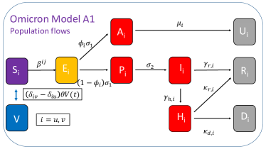
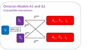
Figure 1: Schematic diagram of population flows according to model A1 (left panel) and susceptible interactions with other population compartments, for both models A1 and A2 (right panel). The symbol $\delta_{ij}$ with $i,j=u,v$ is the Kronecker delta.

While these populations were also present in our earlier work [20], it is relevant to highlight the differences of the omicron-variant modeling. For the period under consideration (fall 2021 to spring 2022), vaccines had been deployed extensively in Andalusia and Switzerland. More importantly, breakthrough infections due to the omicron variant were substantial within the vaccinated population (contrary to the case of the delta variant considered in Section III). In light of that, we formulated two sets of populations: one representing unvaccinated individuals, denoted by (the subscript) $u$, and the other representing the substantial population of vaccinated individuals, denoted by (the subscript) $v$. Each population subset had its own set of parameters. This division of the whole population into two almost independent subgroups (they interact only through the vaccinated time series) is reflected in the presentation of the model schematic in Fig. 1. In fact, Fig. 1 summarizes population flows and interactions: the left panel illustrates the main population compartments and the corresponding flows, while the right panel shows the interactions of susceptibles with other compartments, both for vaccinated and unvaccinated populations. The model equations are:

$$\frac{\mathrm{d}S_{u}}{\mathrm{d}t} =-\beta^{uu}S_{u}(I_{u}+A_{u}+P_{u})-\beta^{uv}S_{u}(I_{v}+A_{v}+P_{v})-\theta V(t),$$ (1a)

$$\frac{\mathrm{d}E_{u}}{\mathrm{d}t} =-\sigma_{1}E_{u}+\beta^{uu}S_{u}(I_{u}+A_{u}+P_{u})+\beta^{uv}S_{u}(I_{v}+A_{v}+P_{v}),$$ (1b)

$$\frac{\mathrm{d}P_{u}}{\mathrm{d}t} =(1-\phi_{u})\sigma_{1}E_{u}-\sigma_{2}P_{u},$$ (1c)

$$\frac{\mathrm{d}A_{u}}{\mathrm{d}t} =\phi_{u}\sigma_{1}E_{u}-\mu_{u}A_{u},$$ (1d)

$$\frac{\mathrm{d}U_{u}}{\mathrm{d}t} =\mu_{u}A_{u},$$ (1e)

$$\frac{\mathrm{d}I_{u}}{\mathrm{d}t} =\sigma_{2}P_{u}-(\gamma_{r,u}+\gamma_{h,u})I_{u},$$ (1f)

$$\frac{\mathrm{d}H_{u}}{\mathrm{d}t} =\gamma_{h,u}I_{u}-(\kappa_{r,u}+\kappa_{d,u})H_{u},$$ (1g)

$$\frac{\mathrm{d}R_{u}}{\mathrm{d}t} =\gamma_{r,u}I_{u}+\kappa_{r,u}H_{u},$$ (1h)

$$\frac{\mathrm{d}D_{u}}{\mathrm{d}t} =\kappa_{d,u}H_{u},$$ (1i)

$$\frac{\mathrm{d}S_{v}}{\mathrm{d}t} =-\beta^{vv}S_{v}(I_{v}+A_{v}+P_{v})-\beta^{vu}S_{v}(I_{u}+A_{u}+P_{u})+\theta V(t),$$ (1j)

$$\frac{\mathrm{d}E_{v}}{\mathrm{d}t} =-\sigma_{1}E_{v}+\beta^{vv}S_{v}(I_{v}+A_{v}+P_{v})+\beta^{vu}S_{v}(I_{u}+A_{u}+P_{u}),$$ (1k)

$$\frac{\mathrm{d}P_{v}}{\mathrm{d}t} =(1-\phi_{v})\sigma_{1}E_{v}-\sigma_{2}P_{v},$$ (1l)

$$\frac{\mathrm{d}A_{v}}{\mathrm{d}t} =\phi_{v}\sigma_{1}E_{v}-\mu_{v}A_{v},$$ (1m)

$$\frac{\mathrm{d}U_{v}}{\mathrm{d}t} =\mu_{v}A_{v},$$ (1n)

$$\frac{\mathrm{d}I_{v}}{\mathrm{d}t} =\sigma_{2}P_{v}-(\gamma_{r,v}+\gamma_{h,v})I_{v},$$ (1o)

$$\frac{\mathrm{d}H_{v}}{\mathrm{d}t} =\gamma_{r,v}I_{v}-(\kappa_{r,v}+\kappa_{d,v})H_{v},$$ (1p)

$$\frac{\mathrm{d}R_{v}}{\mathrm{d}t} =\gamma_{h,v}I_{v}+\kappa_{r,v}H_{v},$$ (1q)

$$\frac{\mathrm{d}D_{v}}{\mathrm{d}t} =\kappa_{d,v}H_{v}.$$ (1r)

We made a number of simplifying assumptions to reduce the number of parameters and enhance the identifiability of the model (see also the relevant analysis in Appendix A). We consider a model with only four transmission rates $\beta^{ij}(i,j=u,v)$. We assumed that infectious contacts could only occur between four groups: between unvaccinated individuals (unvaccinated-unvaccinated contacts denoted by the superscript $uu$), between vaccinated and vaccinated individuals (denoted by the superscript $vv$) and across these two groups (denoted by $uv$ —for vaccinated transmitting to unvaccinated and $vu$ for the reverse path of infection). Notice that $uv$ and $vu$ are not a priori assumed to be equivalent. Within each subgroup of infection transmission ($uu,vv$, $uv$, and $vu$), the infections induced by the three infectious compartments $P$, $A$ and $I$ are assumed to occur at the same rate, i.e., the transmission rate is considered to be independent of whether the infectious individual exhibits symptoms ($I$) or not ($A,P$). While we expect these transmission rates to differ (in fact, we know that even within a given population the $S-I$ transmission rate differs from the $S-A$ transmission rate, see for example, Ref. [20]), the identifiability analysis based on the available time series suggests that they would not be independently computable in a definitive way. In addition, we introduced a single constraint that requires that the incubation period of the disease $\tau_{\textrm{inc}}=\sigma_{1}^{-1}+\sigma_{2}^{-1}$ be a value randomly sampled from a normal distribution with mean 3.42 and standard deviation 0.2755. This leverages information about the (shorter) incubation period associated with the omicron variant [23].

Vaccine efficiency is introduced via the parameter $\theta$, whose variation bounds were set in the range 75%–95%. This factor multiplied by the time series of vaccinations $V(t)$ effectively “transfers” individuals from the unvaccinated susceptible population to the vaccinated susceptible compartment. It is important to remark that $H$ measures both conventional and critical hospitalizations together. While we recognize the relevance of the ongoing debate of distinguishing deaths “from COVID” vs. “with COVID” [24], unfortunately the data available herein do not allow for a definitive distinction between the two.

We obtained the best-fit parameters and initial conditions by minimizing an appropriately chosen norm. For both regions of interest, the time period used for the fits was from November 15, 2021 to March 1, 2022. The identification of the date a particular variant appeared in a geographical location is fraught with uncertainties.The choice of November 15, 2021 as the initial day of fittings stems from a number of indirect indications: Ref. [25] reports a surge of cases in Germany at the beginning of November; Ref. [26] mentions that an omicron-variant case was reported on November 19; and the WHO site [27] mentions that in South Africa the first confirmed infection was reported on November 24, although arising in the sequencing of a sample collected on November 9. Additionally, inspection of the data shows a gradual increase starting at November 15, after a plateau. The effective parameter training period indicated above (till March 1, 2022), is followed by a prediction period (with the optimal parameters and initial conditions fixed, as determined in the training period). The predicted time series that terminates on March 29, 2022 is then compared to the reported data. Predictions do not go beyond that date because the measurement strategy in Andalusia changed, thereby rendering our fixed parameters of limited relevance to the new data. Moreover, around that time Spanish public policy also changed, and face masks were no longer required. In Switzerland some restrictions were removed in the middle of February. More details are presented in the appropriate results sections.

We perform two separate fits, i.e., we used two different norms to compare predictions to reported numbers depending on data availability. First, we fit the predicted total number of fatalities to the reported number by minimizing the norm $\mathcal{N}$ (i.e., the loss function)

$${\mathcal{N}}=\frac{1}{n}\sum_{i=1}^{n}\Big{\{}\log\big{[}D_{u,\mathrm{num}}(t_{i})+D_{v,\mathrm{num}}(t_{i})\big{]}-\log\big{[}D_{\mathrm{obs}}(t_{i})\big{]}\Big{\}}^{2},$$ (2)

where the subscript “num” refers to predicted (calculated) numbers and “obs” to observation (reported numbers), and $n$ refers to the number (days) of observations. This loss function effectively does not distinguish the compartmental origin of the fatalities, i.e., whether they arise from the $u$ or $v$ compartments: it only accounts for the cumulative number of fatalities. This will, inevitably, result in the determination of some parameters between the unvaccinated and the vaccinated populations that may not necessarily be epidemiologically meaningful (as we will see in the detailed comparisons of our predictions for Andalusia and Switzerland).

Whenever we used norm (2), we also included the waning effect of the vaccines and booster vaccination effects, in addition to those fully vaccinated. It is well-documented that different vaccines have different waning immunities (see, for instance, the detailed analysis of Ref. [28]). However, to be able to account for these effects without adding a large number of additional coefficients, we assumed that vaccines are roughly effective for an interval of about 180 days. Consequently, we define $V(t)$ as:

$$V(t)=V_{fv}([t])-V_{fv}([t-180])+V_{b}([t]),$$ (3)

where the subscripts $fv$ refers to fully vaccinated, and $b$ to booster.

The above optimization via norm (2) is a point estimator, that is, a single set of parameters and initial conditions is obtained. To calculate their confidence intervals, and consequently the confidence interval of the predictions, we follow the bootstrapping method described in [29]. The first step is to generate 250 random, synthetic, time series for the fatalities based on the reported data. To accomplish this, we first apply the optimization to find the best fit to the original data set: we refer to that optimization of the reported fatalities data as the “numerical truth”. In this first optimization, we also included $I_{u}(0)$, $I_{v}(0)$, $E_{u}(0)$, $E_{v}(0)$, $A_{u}(0)$, $A_{v}(0)$, $H_{u}(0)$ and $H_{v}(0)$ as fitting parameters: these parameters were fixed in the subsequent bootstrapping steps. Then, random noise of a prescribed level, empirically chosen to be 5%, was added to the “numerical truth” to generate 250 “polluted” (i.e., noisy) time series for the fatalities. Knowledge of the error in data collection may be helpful to select an appropriate noise level. In the second step, we apply the optimization procedure to find the best fit to each of the 250 synthetic fatalities time series to obtain 250 sets of parameters from which the confidence intervals for the parameters and predictions can be computed. The same bootstraping procedure was used for the hospitalization time series.

We also fitted separately, if the reported data allowed us, the vaccinated and unvaccinated fatalities time series using them as separate inputs to our minimization objective. In that case, the relevant norm is

$${\mathcal{N}}=\frac{1}{n}\sum_{i=1}^{n}\Big{\{}\log\big{[}D_{u,\mathrm{num}}(t_{i})\big{]}-\log\big{[}D_{u,\mathrm{obs}}(t_{i})\big{]}\Big{\}}^{2}+\Big{\{}\log\big{[}D_{v,\mathrm{num}}(t_{i})\big{]}-\log\big{[}D_{v,\mathrm{obs}}(t_{i})\big{]}\Big{\}}^{2}.$$ (4)

With this norm, we are genuinely treating the vaccinated compartment separately: we expect its fraction of fatalities (proportionally to the corresponding susceptible population) to be reflected in the obtained parameters. It should be added that in this case, given the way that the data are obtained, the vaccinated status corresponds to people who had received the full doses, independently of antibodies waning, boosting, or efficacy of vaccines. Consequently, $\theta$ has been fixed to 1 in every fit, and $V(t)$ is defined as

$$V(t)=V_{fv}([t]).$$ (5)

We mention here that an important consideration pertinent to the model concerns the identifiability of its coefficients (and initial conditions). This pertains to whether, based on the time series given, the unknown model parameters can be uniquely identified [30]. In addition to the question whether all parameters can be uniquely identified (global identifiability) or some may have multiple possible values (local identifiability), there are also practical issues concerning whether different sets of parameters lead to similar (although not necessarily identical) observations; see, e.g., the discussion of [31]. Here, following the approach presented in Appendix A (see also [32, 33, 34]), we find that all the parameters are globally identifiable, except

$$\gamma_{h,u},\quad\gamma_{r,u},\quad\gamma_{h,v},\quad\gamma_{r,v},\quad\kappa_{d,u},\quad\kappa_{r,u},\quad\kappa_{d,v},\quad\kappa_{r,v}.$$

For these eight parameters, the following combinations are globally identifiable:

$$\gamma_{h,u}+\gamma_{r,u},\quad\gamma_{h,v}+\gamma_{r,v},\quad\kappa_{d,u}+\kappa_{r,u},\quad\kappa_{d,v}+\kappa_{r,v},\quad\gamma_{h,u}\kappa_{d,u},\quad\gamma_{h,v}\kappa_{d,v}.$$

As concerns the initial conditions, $H_{u}(0)$ and $H_{v}(0)$ are not identifiable, in addition to the initial conditions for the terminal compartments $U_{u},U_{v},R_{u},R_{v}$.

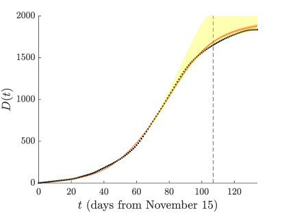
Figure 2: Omicron-variant model A1: Fit and prediction for the total number of fatalities in Andalusia (norm of Eq. (2)). The calculated curve is plotted in red along with its confidence/prediction intervals: red shade corresponds to the interquartile range, while the yellow shade corresponds to the 95% confidence interval comprised between the 2.5 and 97.5 percentiles. Reported data for the total number of fatalities are given by the black points. The vertical line, the beginning of the prediction interval, is March 1, 2022.

The identifiability analysis suggests that $\phi_{u},\phi_{v}$ and many other parameters are globally identifiable, i.e., they have a unique value given the functions $D_{u}(t)$ and $D_{v}(t)$. However, these theoretical-analysis results do not exactly transfer to numerical calculations for various reasons. A globally identifiable parameter may not necessarily have a sharp estimate due to the potential sloppiness [35] of the model. When the output functions are not sensitive to a particular parameter, a sharp estimate will not be expected, even though the parameter may be globally identifiable. Many other factors, e.g., the reliability and accuracy of the reported time series, may exacerbate the situation. The identifiability analysis assumes that both functions $D_{u}(t)$ and $D_{v}(t)$ are outputs, which includes much more information than the simple loss term Eq. (4) can provide. It is an open question how close these estimates are to the actual parameters. Interestingly, however, we find that these estimates still give fairly accurate predictions, even though certain parameter estimates may not be as sharp as desired. When the total death, $D_{u}(t)+D_{v}(t)$, is the only output, we cannot obtain any identifiability results. The implications of there remarks on model identifiability are further elaborated in our comments of best-fit parameters.

II.1.1 Andalusia

Table 1: Optimal parameters and initial conditions for the omicron-variant models in Andalusia: Model fits to the total number of fatalities, discussed in Section II.1.1 (model A1, third column) and to the total number of hospitalizations, discussed in Section II.2.1 (model A2, right column). Population $N_{\textrm{And}}=8.4M$.

Parameter	Symbol	Median (interquartile range)	Median (interquartile range)
		Fit to total number of deaths	Fit to total number of hospitalizations
		[Model A1, norm Eq. (2)]	[Model A2, norm Eq. (7)]
Transmission rate $uu$ [per day]	$\beta^{uu}$	0.6437 (0.6313–0.6532)	0.1279 (0.1134–0.1491)
Transmission rate $uv$ [per day]	$\beta^{uv}$	0.3687 (0.3040–0.4044)	0.0209 (0.0166–0.0270)
Transmission rate $vu$ [per day]	$\beta^{vu}$	0.0679 (0.0591–0.0822)	0.2400 (0.1775–0.2855)
Transmission rate $vv$ [per day]	$\beta^{vv}$	0.1939 (0.1839–0.2168)	0.4516 (0.4381–0.4637)
Latency period [days]	$1/\sigma_{1}$	1.7923 (1.6999–1.8935)	1.8143 (1.7266–1.9164)
Preclinical period [days]	$1/\sigma_{2}$	1.6467 (1.5513–1.7496)	1.6300 (1.5038–1.7509)
$A_{u}/P_{u}$ partitioning	$\phi_{u}$	0.3689 (0.3639–0.3832)	0.3592 (0.3486–0.3743)
$A_{u}/P_{u}$ partitioning	$\phi_{v}$	0.3363 (0.3311–0.3457)	0.3933 (0.3816–0.4063)
Infectivity period ($A_{u}$) [days]	$1/\mu_{u}$	2.9185 (2.8497–2.9433)	3.1540 (3.0764–3.2333)
Recovery rate $I_{u}\rightarrow R_{u}$ [[per day]	$\gamma_{r,u}$	0.1999 (0.1958–0.2103)	0.1998 (0.1871–0.2082)
Transition rate $I_{u}\rightarrow H_{u}$ [per day]	$\gamma_{h,u}$	0.0056 (0.0050–0.0060)	0.0068 (0.0062–0.0072)
Infectivity period ($A_{v}$) [days]	$1/\mu_{v}$	3.2038 (3.1581–3.2467)	3.3018 (3.1663–3.6227)
Recovery rate $I_{v}\rightarrow R_{v}$ [per day]	$\gamma_{r,v}$	0.1728 (0.1692–0.1802)	0.2088 (0.2023–0.2153)
Transition rate $I_{v}\rightarrow H_{v}$ [per day]	$\gamma_{h,v}$	0.0057 (0.0051–0.0064)	0.0015 (0.0014–0.0017)
Recovery rate $H_{u}\rightarrow R_{u}$ [per day]	$\kappa_{r,u}$	0.3436 (0.3314–0.3576)	—
Death rate $H_{u}\rightarrow D_{u}$ [per day]	$\kappa_{d,u}$	0.0090 (0.0080–0.0106)	—
Recovery rate $H_{v}\rightarrow R_{v}$ [per day]	$\kappa_{r,v}$	0.3354 (0.3198–0.3506)	—
Death rate $H_{v}\rightarrow D_{v}$ [per day]	$\kappa_{d,v}$	0.0097 (0.0092–0.0101)	—
Vaccine efficieny [-]	$\theta$	0.8825 (0.8767–0.8885)	0.8510 (0.8436–0.8598)
Initial condition
Initial unvaccinated Exposed ($E_{u}$) population [#]	$E_{u}(0)$	641	1485
Initial unvaccinated Presymptomatic ($P_{u}$) population [#]	$P_{u}(0)$	2217	1541
Initial unvaccinated Asymptomatic ($A_{u}$) population [#]	$A_{u}(0)$	2273	1124
Initial unvaccinated symptomatically Infected ($I_{u}$) population [#]	$I_{u}(0)$	2677	2438
Initial unvaccinated Hospitalized ($H_{u}$) population [#]	$H_{u}(0)$	60	—
Initial vaccinated Exposed ($E_{v}$) population [#]	$E_{v}(0)$	840	3218
Initial vaccinated Presymptomatic ($P_{v}$) population [#]	$P_{v}(0)$	2902	3339
Initial vaccinated Asymptomatic ($A_{v}$) population [#]	$A_{v}(0)$	2976	2435
Initial vaccinated symptomatically Infected ($I_{v}$) population [#]	$I_{v}(0)$	3504	5281
Initial vaccinated Hospitalized ($H_{v}$) population [#]	$H_{v}(0)$	370	—

As mentioned, the fitting time window we used to obtain the optimized parameters and initial conditions was from November 15, 2021 to March 1, 2022. The prediction interval ended on March 29, 2022. The time series for Andalusia is available from the Spanish Health Ministry, but we used the series compiled at [36]. Note that in Andalusia the reported values of $D(t)$, and the total number of hospitalizations $J(t)$, the latter discussed in Section II.2, correspond to the event day, whereas for Switzerland they correspond to the report day.

The vaccination data until April 29, 2021 were also taken from [36]. After that date, they were extracted from the Regional Government of Andalusia (Junta de Andalucía, Ref. [37]). We ignored the vaccinations for kids under 12 years old, as there were many data anomalies, resulting in a time series that appears to be problematic. Irrespective of that, this population segment corresponds to only $\lesssim 4$% of the total vaccinations. The fatalities time series we used did not report how many fatalities could be attributed to vaccinated or unvaccinated individuals. Therefore, for the region of Andalusia we used only norm (2), coupled to the modified vaccination time series as described in Eq. (3), to perform the optimizations.

Figure 2 shows the calculated fatalities time series (both fitting and prediction intervals) and the reported numbers. Table 1 (model A1 in column 3) presents the optimized parameters and initial conditions. The reported interquantile range arises from 250 fits in the bootstraping step, as discussed above.

We observe that the overall trend of the fatalities seems to be reasonably well captured by the model within its prediction intervals (and their associated uncertainty). We do note, however, a slight over-prediction towards the end of the time series, during March 2022. The transmission rates $\beta^{ij}$ ($i,j=u,v$) with at least one member of the unvaccinated population $uu$ and $uv$ are clearly higher than the $vv$ rate between members of the vaccinated population. In fact, $\beta^{uu}$ is more that three times higher than $\beta^{vv}$. The lowest transmission rate is predicted to be $\beta^{vu}$, even lower that $\beta^{vv}$. At this point it is important to recall our discussion about the use of the total number of deaths and the resulting inability to identify definitively the model parameters. Hence, the above numbers, even when they appear to be intuitively relevant, should be taken with a grain of salt. The latency period is approximately 3.5 days, as imposed by our constraint, and in agreement with [23]. The role of asymptomatics, as reflected by the fraction $\phi_{i}$ of exposed who become asymptomatics, is considerable, approximately 1/3 and independent of whether the population is vaccinated or not. The calculated fraction of asymptomatics is in reasonable agreement with Ref. [38] who reported a pooled fraction of asymptomatics for the omicron variant of 25.5% (95% confidence interval 17.0% -38.2%). The vaccinated and unvaccinated infectivity period for asymptomatic infections $1/\mu_{i}$ is approximately constant, at about three days, again independent of whether the $u$ or $v$ compartment is considered.

We also find that some parameters are more difficult to justify, Specifically, we find that the recovery rates of symptomatically infected individuals $I_{i}\rightarrow R_{i}$ and that of the hospitalized individuals $H_{i}\rightarrow R_{i}$ are almost independent of whether the population is vaccinated or not. The same holds for the transition rates $I_{i}\rightarrow H_{i}$ and the death rates $H_{i}\rightarrow D_{i}$: all four of them are found to have weak variations. The independence of these rates on the administration of the vaccine might be related to the norm we used that does not distinguish between fatalities of vaccinated or unvaccinated individuals. We will return to this point in our analysis of the Switzerland data.

II.1.2 Switzerland

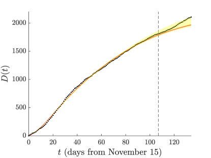
Figure 3: Omicron-variant model A1: Fit and prediction for the total number of fatalities in Switzerland (norm Eq. (2)). The calculated curve is plotted in red along with its confidence/prediction intervals: red shade corresponds to the interquartile range, while the yellow shade corresponds to the 95% confidence interval comprised between the 2.5 and 97.5 percentiles. Reported data for the total number of fatalities are given by the black points. The vertical line, the beginning of the prediction interval, is March 1, 2022.

We chose to perform model calculations for a territory with a population similar in number to that of Andalusia, and for which adequate data are available. As such, we chose a region that contains Switzerland and the Principality of Liechtenstein (data are jointly reported) since the total population of this aggregate territory is 8.7M, (compared to 8.4M for Andalusia). Overall, we followed a procedure very similar to what we used for Andalusia, with a few minor changes. Identical fitting and prediction intervals are used as those for Andalusia. We do note, however, that starting February 17, 2022 most restrictions were lifted in Switzerland. We believe this is one of the reasons we observe a model under-prediction of the number of fatalities in Fig. 3 and in Figs. 4.

Case reporting was slightly different. The Swiss government through the Federal Office of Public Health provides daily the status (vaccinated, unvaccinated or unknown) of each hospitalized/deceased person at Ref. [39]. In the absence of a concrete metric on how to partition unknown fatalities to vaccinated and unvaccinated individuals, we used the following procedure to convert these three time series into two, one associated with vaccinated $D_{v}(t_{i})$ and the other to unvaccinated individuals $D_{u}(t_{i})$. Let $\bar{d}_{v}(t_{i})$, $\bar{d}_{u}(t_{i})$ and $\bar{d}_{\star}(t_{i})$ denote the number of daily reported fatalities with vaccinated, unvaccinated, and unknown state, respectively. We randomly sample an integer number $\delta_{i}\in[0,\bar{d}_{\star}(t_{i})]$, following a uniform distribution, and then we define the daily number of vaccinated/unvaccinated deceased as $d_{v}(t_{i})=\bar{d}_{v}(t_{i})+\delta_{i}$ and $d_{u}(t_{i})=\bar{d}_{u}(t_{i})+[\bar{d}_{\star}(t_{i})-\delta_{i}]$. The total number of deaths is the cumulative sum, i.e. $D_{v}(t_{i})=\sum_{j=1}^{i}d_{v}(t_{j})$ and $D_{u}(t_{i})=\sum_{j=1}^{i}d_{u}(t_{j})$. Note that we followed the same procedure to generate the hospitalizations $J_{v}$ and $J_{u}$ used in model A2, in Section II.2.2. As mentioned earlier, $D(t)$ and $J(t)$ for Switzerland correspond to the report day.

Given the reconstructed time series $D_{i}(t)$ we used norm (4), in addition to the norm (2) used in the case of Andalusia, to fit and predict the fatalities time series for the territory of Switzerland (and the Pricipality of Liechtenstein). We attempted to fit separately the vaccinated and unvaccinated deceased, using them as separate inputs to our minimization objective. As mentioned earlier, since we consider that vaccinated individuals have received the full dose (neglecting immunity waning, boosting, of vaccine efficiency) we take $\theta=1$ in every fit, and $V(t)$ is defined as described in Eq. (5). Our results for the fit to the total number of fatalities are shown in Fig. 3, whereas those for the separate fits to vaccinated and unvaccinated deaths are presented in Fig. 4. Table 2, columns two and four, presents the fitting parameters and initial conditions.

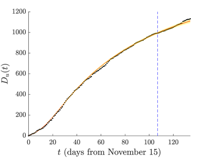
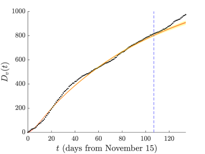
Figure 4: Omicron-variant model A1: Separate fits of vaccinated and unvaccinated fatalities in Switzerland (norm Eq. (4)). Left panel: Fatalities of vaccinated individuals. Right panel: Fatalities of unvaccinated individuals. Calculated curves are plotted in red along with its confidence/prediction intervals: red shade corresponds to the interquartile range, whereas the yellow shade presents the 95% confidence interval comprised between the 2.5 and 97.5 percentiles. Reported data for the total number of vaccinated and unvaccinated fatalities are given by the black points. The vertical line, the beginning of the prediction interval, is March 1, 2022.

We can see a clear model under-prediction of the fatalities (within the testing period), for both optimizations (norm (2) and (4)), despite an accurate following of the time-series trend throughout the period over which regression is performed. The under-prediction is more severe in the case of the total number of fatalities, Fig. 3, and in the vaccinated death time series of the right panel in Fig. 4. As mentioned earlier, we attribute the under-prediction to the fact that after the end of the fitting period, restrictions were considerably relaxed leading to more cases, and eventually more fatalities, a feature that was not explicitly factored in the model.

As regards the parameters of the model, we observe very similar trends to what we obtained for Andalusia. A notable exception is that in the total-deaths fit $\beta^{uv}$ is the highest transmission rate, retaining however $\beta^{uu}\gg\beta^{vv}$ in the case of norm (2). The latency period is well reproduced (as expected due to the constraint and Ref. [23]), and the fraction of asymptomatics is approximately 25% (again in agreement with [38]) irrespective of vaccination or not. The remaining parameters follow similar trends as reported in Table 1 for Andalusia. It is noteworthy that in both cases recovery, transmission, and death rates seem to depend relatively weakly on whether the vaccine had been administered or not.

A comparison of the parameters predicted by the two optimization is in order. When the two distinct populations are used in the regression, we observe, in the third column in Table 2, that the transition rate $\beta^{vv}$ becomes the largest one with $\beta^{vu}$ being the smallest. While a calculated higher viral transmissivity of vaccinated individuals could, in principle, be attributed to taking fewer measures to limit pathogen transmission via behavioral changes, e.g., higher contact rates, negligence to use face masks, etc, it is not obvious that such an attribution is meaningful, rather than the potential outcome of the sloppiness of the model. Another surprising feature is that we do not find a significant dependence of the parameters on the norm used (apart from the noted difference in the transmission rates). The asymptomatic fraction is predicted to be slightly larger, approximately 30%, the $H_{u}\rightarrow R_{u}$ is slightly smaller, and the death rate is slightly larger.

Table 2: Optimal parameters and initial conditions for the omicron-variant models in Switzerland: Model fits to (a) the total number of fatalities (model A1, second column from the left), (b) the total number of hospitalizations (model A2, third column), (c) to the $u,v$ total number of fatalities separately (model A1, fourth column), and (d) to the $u,v$ total number of hospitalizations separately (model A2, fifth column). Population $N_{\textrm{CHL}}=8.7M$. Parameters descriptions are as defined in Table 1.

Parameter	Median (interquartile range)	Median (interquartile range)	Median (interquartile range)	Median (interquartile range)
	Fit: total number of deaths	Fit: total hospitalizations	Fit: $u,v$ deaths separately	Fit: $u,v$ hospitalizations separately
	[Model A1, norm Eq. (2)]	[Model A2, norm Eq. (7) ]	[Model A1, norm Eq. (4)]	[Model A2, norm Eq. (8)]
$\beta^{uu}$	0.1682 (0.1491–0.1915)	0.2563 (0.2241–0.2855)	0.1607 (0.1339–0.1862)	0.3418 (0.3300–0.3539)
$\beta^{uv}$	0.2450 (0.2088–0.2840)	0.2084 (0.1798–0.2328)	0.2023 (0.1840–0.2235)	0.1509 (0.1216–0.1846)
$\beta^{vu}$	0.0780 (0.0541–0.0979)	0.0709 (0.0357–0.0995)	0.0261 (0.0158–0.0399)	0.0500 (0.0453–0.0551)
$\beta^{vv}$	0.0977 (0.0790–0.1144)	0.1422 (0.1123–0.1711)	0.2266 (0.1917–0.2625)	0.1885 (0.1737–0.2037)
$1/\sigma_{1}$	1.7558 (1.6627–1.8545)	1.7605 (1.6190–1.9650)	1.7811 (1.6837–1.8945)	1.7169 (1.6315–1.8140)
$1/\sigma_{2}$	1.6798 (1.5660–1.8040)	1.6690 (1.4572–1.8302)	1.6384 (1.5075–1.7495)	1.7085 (1.5905–1.8255)
$\phi_{u}$	0.2469 (0.2333–0.2588)	0.2659 (0.2472–0.2865)	0.3125 (0.2885–0.3366)	0.3360 (0.2880–0.3803)
$\phi_{v}$	0.2551 (0.2465–0.2617)	0.2680 (0.2546–0.2834)	0.3346 (0.3063–0.3535)	0.3161 (0.2936–0.3337)
$1/\mu_{u}$	3.1794 (3.0941–3.2628)	3.1836 (3.0829–3.3157)	3.2599 (3.1700–3.4231)	3.4953 (3.2164–3.9040)
$\gamma_{r,u}$	0.1509 (0.1335–0.1661)	0.1845 (0.1678–0.2006)	0.1386 (0.1263–0.1511)	0.1731 (0.1562–0.1867)
$\gamma_{h,u}$	0.0115 (0.0091–0.0133)	0.0037 (0.0034–0.0042)	0.0107 (0.0093–0.0121)	0.0039 (0.0038–0.0041)
$1/\mu_{v}$	3.2920 (3.2141–3.4560)	3.3012 (3.1761–3.4442)	3.0606 (2.8636–3.2685)	3.2347 (3.0419–3.4284)
$\gamma_{r,v}$	0.1607 (0.1431–0.1707)	0.1679 (0.1357–0.1892)	0.1627 (0.1469–0.1892)	0.1424 (0.1315–0.1571)
$\gamma_{h,v}$	0.0106 (0.0095–0.0120)	0.0028 (0.0025–0.0031)	0.0105 (0.0095–0.0118)	0.0029 (0.0028–0.0029)
$\kappa_{r,u}$	0.2521 (0.2216–0.2852)	—	0.1882 (0.1515–0.2290)	—
$\kappa_{d,u}$	0.0185 (0.0162–0.0207)	—	0.0186 (0.0178–0.0193)	—
$\kappa_{r,v}$	0.1886 (0.1314–0.2738)	—	0.1688 (0.1576–0.1808)	—
$\kappa_{d,v}$	0.0071 (0.0060–0.0084)	—	0.0109 (0.0102–0.0116)	—
$\theta$	0.8483 (0.8417–0.8552)	0.8662 (0.8529–0.8871)	1	1
Initial condition
$E_{u}(0)$	5648	8234	2690	6483
$P_{u}(0)$	4767	4340	2677	5530
$A_{u}(0)$	3609	3762	988	3110
$I_{u}(0)$	11318	12759	5189	12655
$H_{u}(0)$	295	—	278	—
$E_{v}(0)$	9401	8642	10330	6477
$P_{v}(0)$	7936	4555	10278	5524
$A_{v}(0)$	6007	3949	3795	3107
$I_{v}(0)$	18839	13392	19925	12644
$H_{v}(0)$	381	—	200	—

II.2 Model A2: Branches terminate at hospitalizations

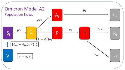
Figure 5: Schematic diagram of the population flows according to model A2. The susceptible interactions are as in model A1, shown in the the right panel of Fig. 1. The symbol $\delta_{ij}$ with $i,j=u,v$ is the Kronecker delta.

We now consider model A2, an omicron-variant model similar to A1, but where the population branches terminate at the total number of hospitalizations. The total hospitalization data appear, in our gauge, to be more reliable than fatalities, as the latter (at least in Andalusia) include deceased by any cause that may have recently generated a positive test. That is to say, we believe that numerous fatalities were attributed to COVID even though the primary reason for these events had not been COVID, but another occurrence, see, for example, [40]. By considering the reported (total, conventional and critical) hospitalizations, this possible misattribution of fatalities to COVID-19 may be diminished.

Model A2 is the same as model A1 described by Eqs. (1), differing only in the terminal compartments of hospitalizations. This implies that the ODEs Eqs.(1a)–(1f) and Eqs. (1j)–(1o) form part of the model A2 equations, as well. However, Eqs. (1g)–(1i) and Eqs. (1p)–(1r) are to be replaced by

$$\begin{split}\frac{\mathrm{d}J_{i}}{\mathrm{d}t}&=\gamma_{h,i}I_{i},\quad i=u,v,\\ \frac{\mathrm{d}R_{i}}{\mathrm{d}t}&=\gamma_{r,i}I_{i},\quad i=u,v\end{split}$$ (6)

where $J(t)$ in the total number of hospitalizations and $\gamma_{ij}$ is the rate symptomatically infected individuals $u,v$ become hospitalized $\gamma_{h,i}$ or recover $\gamma_{r,i}$.

The optimal parameters (and initial conditions) are obtained by a procedure similar to what we used in model A1 with $J(t)$ playing the role of $D(t)$. Accordingly, the norms change: Eq. (2) becomes

$${\mathcal{N}}=\frac{1}{n}\sum_{i=1}^{n}\Big{\{}\log\big{[}J_{u,\mathrm{num}}(t_{i})+J_{v,\mathrm{num}}(t_{i})\big{]}-\log\big{[}J_{\mathrm{obs}}(t_{i})\big{]}\Big{\}}^{2},$$ (7)

while Eq. (4) becomes

$${\mathcal{N}}=\frac{1}{n}\sum_{i=1}^{n}\Big{\{}\log\big{[}J_{u,\mathrm{num}}(t_{i})\big{]}-\log\big{[}J_{u,\mathrm{obs}}(t_{i})\big{]}\Big{\}}^{2}+\Big{\{}\log\big{[}J_{v,\mathrm{num}}(t_{i})\big{]}-\log\big{[}J_{v,\mathrm{obs}}(t_{i})\big{]}\Big{\}}^{2}.$$ (8)

II.2.1 Andalusia

The results of fitting the total hospitalizations (arising from both vaccinated plus unvaccinated populations using norm (7)) are shown in Figure 6. The optimal parameters and initial conditions are summarized in Table 1, last column.

As in the case of the cumulative optimization of both the vaccinated and the unvaccinated fatalities, the results of Fig. 6 appear quite accurate, including the forward prediction for the month of March (despite a slight under-prediction of hospitalizations). Note that model A1 predictions were slightly above reported fatalities. However, a more careful inspection of the obtained parameters suggests that some of them may not be epidemiologically realistic. Inspection of the optimized transmission rates shows that the $vv$ rate is larger than the $uu$ rate ($\beta^{vv}>\beta^{uu}$ and $\beta^{vu}>\beta^{uv}$ and $>\beta^{uu}$). Whereas these inequalities may be related to changes in the behavior of vaccinated individuals, (for example, vaccinated individuals may take fewer precautions and socialize more) we believe instead that this aspect points to the non-identifiability of the model. It is also likely that the origin of these transmission rates stems from our regression’s inability to expressly distinguish between the two $u,v$ compartments,. More concretely, similarly to model A1, the appropriate identifiability analysis should consider that the only output is the cumulative number of hospitalizations $J_{u}(t)+J_{v}(t)$. However, for such an output we could not obtain any identifiability results following the procedure described in Appendix A. The model is too complex and beyond the capability of the current identifiability-analysis packages.

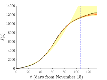
Figure 6: Omicron-variant model A2: Fit and prediction for the total number of hospitalizations in Andalusia (norm of Eq. (7)). The calculated curve is plotted in red along with its confidence/prediction intervals: red shade corresponds to the interquartile range, yellow shade to the 95% confidence interval comprised between the 2.5 and 97.5 percentiles. Reported data for the total number of hospitalizations are given by the black points. The vertical line, the beginning of the prediction interval, is March 1, 2022.

II.2.2 Switzerland

We followed the same procedure as that for Andalusia to generate the model A2 fits and predictions for Switzerland (including the Principality of Liechtenstein). As for model A1, we fitted both the total number of hospitalizations via norm (7) and the two vaccination-identified compartments via norm (8). We followed the same procedure as that used to determine $D_{u}(t)$ and $D_{v}(t)$ to obtain estimates for $J_{u}(t)$ and $J_{v}(t)$.

Figure 7 presents our results for the fit to total number of hospitalizations. Figure  8, instead, corresponds to the vaccinated and unvaccinated populations considered separately in the regression. Table 2, third and fifth column, summarizes all the fitting parameters and initial conditions.

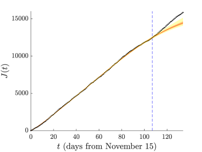
Figure 7: Omicron-variant model A2: Fit and prediction of the total number of hospitalizations in Switzerland (norm of Eq. (2)). The calculated curve is plotted in red along with its confidence/prediction intervals: red shade corresponds to the interquartile range, whereas the yellow shade presents the 95% confidence interval comprised between the 2.5 and 97.5 percentiles. Reported data for the total number of hospitalizations are given by the black points. The vertical line, the beginning of the prediction interval, is March 1, 2022.

We can see a clear model under-prediction of hospitalizations, despite an accurate following of the time-series throughout the period over which regression is performed. The under-prediction is more pronounced in the case of the fit to the total number of hospitalizations. In the case of the separate fittings, the hospitalizations of the vaccinated population are more under-predicted than the hospitalizations of unvaccinated individuals. We attribute this to the fact that, as also discussed in the context of fatalities, towards the end of the fitting period, restrictions were considerably relaxed leading to more cases, and eventually more fatalities. As regards the parameters of the model, we find the transmission rates to be more in line with what one might typically expect. In particular, $\beta^{uu}>\beta^{vv}$ for both fittings (with the two different norms), but $\beta^{uv}>\beta^{vv}$ for the fitting to the total hospitalization, whereas the reverse is true for the fitting to the two separate populations (although in both cases, the rates are fairly similar, even more so when considering the interquartile ranges). The fraction of asymptomatics varies from approximately 27% to 33%, again in reasonable agreement with [38]. The remaining parameters do not seem to significantly depend on the norm chosen.

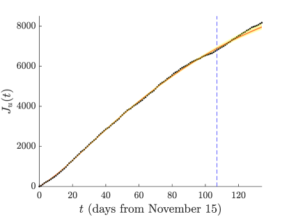
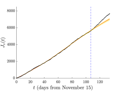
Figure 8: Omicron-variant model A2: Separate fits of vaccinated and unvaccinated hospitalizations in Switzerland (norm Eq. (4)). Left panel: Hospitalizations of vaccinated individuals. Right panel: Hospitalizations of unvaccinated individuals. Calculated curves are plotted in red along with its confidence/prediction intervals: red shade corresponds to the interquartile range, whereas the yellow shade presents the 95% confidence interval comprised between the 2.5 and 97.5 percentiles. Reported data for the total number of vaccinated and unvaccinated hospitalizations are given by the black points. The vertical line, the beginning of the prediction interval, is March 1, 2022.

In our identifiability analysis of model A2 with the two vaccination compartments treated separately we considered, as in the case of model A1, that $J_{u}(t)$ and $J_{v}(t)$ are separately, and continuously, known. Moreover, we took $\theta=1$. In the case of model A2 and under the above assumptions, following the procedure described in Appendix A, we can show that all parameters and initial conditions are globally identifiable. This implies that, in principle, all initial conditions and parameters can be determined from the output $J_{u}(t)$ and $J_{v}(t)$. Practically speaking, however, only the discrete time series $J_{u}(t)$ and $J_{v}(t)$ are known: we do not have the full information of the continuous changes of $J_{u}(t)$ and $J_{v}(t)$ as the identifiability analysis supposes. Hence, the loss function used in the parameter estimation is based on a discrete time series reflecting a finite number of observations. Given the complexity of the model and the large number of parameters involved, the optimization package often fails to find a minimum. To alleviate the situation, we chose to fix certain initial conditions, even though such a choice is inconsistent with being globally identifiable. Combined with the possible sloppiness of the model, the result of such a choice may be that the estimates for some of the parameters may not be as sharp. We indicate the above to mitigate a potential impression (to the reader) that the mathematically obtained global identifiability of the model should be expected to translate into the most definitive model results.

III Delta variant

Having explored the more elaborate model setting of the omicron variant we now turn to the simpler case of the delta variant. What simplifies the model considerably is that it is sufficient to consider a single susceptibles population since infection of vaccinated individuals was rare. Consequently, susceptibles who are vaccinated are added to a “withdrawn” population. An alternative option is to add them to the recovered population in the sense that this is a terminal compartment of the model. For the time period of 3-4 months for which the delta variant was dominant, the potential waning of immunity (either from recovery or from the vaccine) is not considered sufficient to allow these individuals to replenish the susceptibles compartment. For more persistent variants, replenishing the susceptibles population may be relevant.

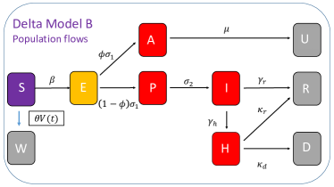
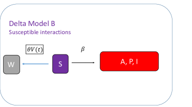
Figure 9: Schematic diagram of population flows according to the delta-variant model B (left panel) and susceptible interactions with other population compartments (right panel). A single population is modeled, as we consider that the waning immunity time scale (either due to vaccine immunity or due to recovery) is much longer than the time scale of prevalence of the delta variant. Vaccinated individuals W are permanently removed from the susceptible compartment, their population becoming a terminal compartment of the model.

Furthermore, the SARS-CoV-2 vaccines were highly effective against the delta variant, leading to rather few breakthrough infections. This fact removes the need for a detailed modeling of compartments within the vaccinated category. Accordingly, the relevant model with the same (but single-component) populations as before and with the addition of the withdrawn ($W$) compartment reads:

$$\begin{split}\frac{\mathrm{d}S}{\mathrm{d}t}&=-\beta S(I+A+P)-\theta V(t),\\ \frac{\mathrm{d}E}{\mathrm{d}t}&=-\sigma_{1}E+\beta S(I+A+P),\\ \frac{\mathrm{d}P}{\mathrm{d}t}&=(1-\phi)\sigma_{1}E-\sigma_{2}P,\\ \frac{\mathrm{d}A}{\mathrm{d}t}&=\phi\sigma_{1}E-\mu A,\\ \frac{\mathrm{d}U}{\mathrm{d}t}&=\mu A,\\ \frac{\mathrm{d}I}{\mathrm{d}t}&=\sigma_{2}P-(\gamma_{r}+\gamma_{h})I,\\ \frac{\mathrm{d}H}{\mathrm{d}t}&=\gamma_{h}I-(\kappa_{r}+\kappa_{d})H,\\ \frac{\mathrm{d}R}{\mathrm{d}t}&=\gamma_{r}I+\kappa_{r}H,\\ \frac{\mathrm{d}D}{\mathrm{d}t}&=\kappa_{d}H,\\ \frac{\mathrm{d}W}{\mathrm{d}t}&=\theta V(t).\end{split}$$ (9)

A schematic of the population flows (left panel) and the susceptible interactions is shown in Fig. 9.

The initial conditions are taken in a similar fashion as in the omicron variant, except for $S(0)$, which is taken as a fitting parameter. We chose to render it a fitting parameter since susceptibles who became infected with previous variants are immune to the delta variant. However, their number is not definitively known. Moreover, as in our modeling of the omicron variant via models A1 and A2, we supposed that the transmission rate $\beta$ is the same for all three infectious compartments: asymptomatics, presymptomatics, and for the symptomatically infected population. In addition, as in the case of the omicron-variant models, we imposed the single constraint on the incubation period $\tau_{\textrm{inc}}=\sigma_{1}^{-1}+\sigma_{2}^{-1}$ to be equal to a value randomly sampled following a normal distribution whose mean now is 4.41 and standard deviation 0.3291, in line with what is reported in [23].

The norm associated with model B, and minimized during the optimization procedure is:

$${\mathcal{N}}=\frac{1}{n}\sum_{i=1}^{n}\Big{\{}\log\big{[}D_{\mathrm{num}}(t_{i})\big{]}-\log\big{[}D_{\mathrm{obs}}(t_{i})\big{]}\big{\}}^{2}.$$ (10)

Again, following the approach presented in Appendix A, we find that the three parameters $\sigma_{1},\phi,\mu$ and the following combinations

$$(\gamma_{h}+\gamma_{r})+\sigma_{2},\quad(\gamma_{h}+\gamma_{r})\cdot\sigma_{2},\quad\kappa_{d}+\kappa_{r},\quad\frac{\beta(\gamma_{h}+\gamma_{r})}{\gamma_{h}\kappa_{d}},\quad\frac{\gamma_{h}}{\gamma_{h}+\gamma_{r}}\kappa_{d}\theta,$$

are globally identifiable. Thus $\sigma_{2}$ and the sum $(\gamma_{h}+\gamma_{r})$ are locally identifiable. Initial conditions other than $D(0)$, which is explicitly available through the fatality time series, are not identifiable. As discussed in the identifiability analyses of the two omicron models, this is just the theoretical result, based on the analysis of [32]. As we have empirically observed, when we fix certain initial conditions or choose a bound for the parameters to be optimized, the identifiability properties of the model may change. In that light, the relevant parameter identifications should be considered with the associated practical “word of caution” indicated above.

III.1 Andalusia and Switzerland

In our simulations, the fitting window for the Andalusia calculation started on June 15, 2021, whereas it started on July 1, 2021 for the Switzerland simulations. The choice of the initial time was determined from the existence of a plateau in the associated time series. The fitting period ended on October 1, 2021 for both regions, and the prediction interval terminated on November 1, 2021. As mentioned in Section II the omicron variant appeared in November 2021.

Figure 10 shows the results of our model B simulations, both for the fitting and the prediction intervals. The left panel presents results for Andalusia, whereas the right panel for Switzerland. The best fitting parameters and initial conditions for both countries corresponding to the model B ODEs are presented in Table 3.

In the case of Andalusia, we observe a high quality fit, not only for the regression interval but also for the prediction interval. Nevertheless, some parameters do not seem to be in agreement with current knowledge of the epidemiology of the delta variant of SARS-CoV-2. We believe, that the primary reason is the lack of identifiability of the model (both the local aspects thereof theoretically, as well as the practical aspect highlighted above in connection to data and initial condition choices). For example, the recovery time of asymptomatics, $1/\mu$ is found to be $\approx 3.5$ days, and an upper bound to the recovery time of symptomatically infected is $1/\gamma_{r}\approx 5.4$ days. It may be expected that both time scales are likely to be longer than these predictions, although these numbers are in reasonable correspondence with findings, e.g., such as the ones of [41] for the delta variant. On the other hand, the fraction of asymptomatics, 8%, is in agreement with the review and analysis of [38] who found a considerably smaller fraction of asymptomatics associated with the delta than the omicron variants, again in agreement with our calculations.

Our model calculations for Switzerland in Fig. 10 provide a reasonable fit throughout the training interval.: calculations initially under-predict and later over-predict. Nevertheless, the predicted time series considerably under-predicts the number of fatalities over the testing period. Some optimized parameters for this territory differ significantly from those obtained for Andalusia. In particular, the transmission rate for the Switzerland data is higher than that for the Andalusia data, as are the $H\rightarrow R$ recovery rates. The Switzerland parameters, however, for the death rate and the vaccine efficiency are predicted to be lower than those for Andalusia. In this case, we do not have a definitive attribution of the relevant result (i.e., the under-prediction of fatalities) in the case of Switzerland. The only change in policy that we could identify was that from September 13, 2021, access to most indoor public spaces like restaurants, bars, museums or fitness centres was permitted with a valid COVID certificate in Switzerland. No other restrictions were enforced on fully vaccinated and boosted people.

Table 3: Optimal parameters and initial conditions for the delta-variant model, model B, in Andalusia (third column) and Switzerland (fourth column). Model fits to the total number of fatalities, norm (10).

Parameter	Symbol	Median (interquartile range)	Median (interquartile range)
		Andalusia	Switzerland
		Model B, norm (10)	Model B, norm (10)
Transmission rate [per day]	$\beta$	0.4526 (0.4210–0.4703)	0.5445 (0.5320–0.5570)
Latency period [days]	$1/\sigma_{1}$	2.2001 (2.0896–2.2982)	2.2027 (2.1113–2.3021)
Preclinical period [days]	$1/\sigma_{2}$	2.1590 (2.0518–2.2789)	2.2056 (2.1112–2.3055)
$A/P=$ partitioning [-]	$\phi$	0.0801 (0.0780–0.0827)	0.0800 (0.0787–0.0820)
Infectivity period ($A$) [days]	$1/\mu$	3.4493 (3.3551–3.5658)	3.4708 (3.3879–3.6194)
Recovery rate $I\rightarrow R$ [per day]	$\gamma_{r}$	0.1852 (0.1643–0.1982)	0.1888 (0.1842–0.1959)
Transition rate $I\rightarrow H$ [per day]	$\gamma_{h}$	0.0017 (0.0016–0.0020)	0.0026 (0.0024–0.0027)
Recovery rate $H\rightarrow R$ [per day]	$\kappa_{r}$	0.0629 (0.0523–0.0831)	0.2480 (0.2355–0.2637)
Death rate $H\rightarrow D$ [per day]	$\kappa_{d}$	0.0462 (0.0449–0.0481)	0.0069 (0.0066–0.0072)
Vaccine efficiency [-]	$\theta$	0.7956 (0.7802–0.8240)	0.6162 (0.6047–0.6189)
Initial ratio [#]	$S(0)/N(0)$	0.5824 (0.5673–0.5951)	0.5278 (0.5178–0.5377)
Initial conditions
Initial exposed population [#]	$E(0)$	1322	669
Initial presymptomatic population [#]	$P(0)$	351	591
Initial asymptomatic population [#]	$A(0)$	205	332
Initial symptomatically infecgted population [#]	$I(0)$	1914	1441
Initial hospitalized population [#]	$H(0)$	80	57

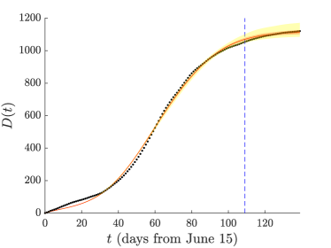
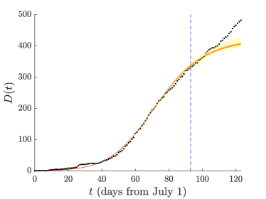
Figure 10: Delta-variant model B: Fit and prediction of the total number of fatalities in Andalusia (left panel) and Switzerland (right panel). Norm (10) was used. The vertical line, the beginning of the prediction interval, is October 1, 2022. Note the significant difference in the number of fatalities.

IV Conclusions and Future Challenges

In this work we presented a new class of compartmental epidemiological models that was motivated by the immunological properties of the delta and omicron variants of SARS-CoV-2. More generally, our aim was to present possibilities for settings where variants are highly transmissive (and hence relevant to consider vaccinated individuals and their epidemiological characteristics) as in the case of models A1-A2 for the omicron variant, as well as ones where breakthrough infections are more rare, and hence vaccination is tantamount to withdrawal from the susceptible population as in the case of model B for the delta variant. We, therefore, constructed model B, with the stipulation that vaccinated individuals were permanently withdrawn from the susceptible population based on the vaccination records and vaccine coverage rate. On the other hand, the epidemiology of the omicron variant suggests a substantial number of breakthrough infections, namely infections of vaccinated individuals. Accordingly, we developed models for both vaccinated and unvaccinated populations and analyzed their pairwise interaction and overall time evolution. Indeed, two classes of regression results were given. In the first (and more crude) regression, only the cumulative number of fatalities was accounted for in the optimization objective. This was done when the data did not allow the partitioning of fatalities (or hospitalizations) to vaccinated and unvaccinated components. In the second, more refined approach, fatalities (or hospitalizations) stemming from the two different (vaccinated or not) groups were separately considered.

We addressed the identifiability of the various models and considered mathematical issues (e.g., parameters globally and locally identifiable, given particular time series), we raised some practical considerations due to the finite nature of the available observations, and we considered the compatibility of the selection of some initial conditions. In the case where the time series associated with vaccinated and unvaccinated individuals are required, we identified the issue of how to handle the so-called “unknown” deaths if the individual vaccination status remains undeclared. We proposed a concrete approach to address such disparities, yet clearly these topics merit further investigation.

In our presentation, we focused on the region of Andalusia in Spain and the country of Switzerland (which included data from the Principality of Liechtenstein). These two territories have similar populations. In each territory, we presented studies of a regression effort involving the fatalities (model A1), as well as one terminating at the compartment of total (i.e., conventional plus critical) hospitalizations (model A2). Our models gave generally good agreement with the corresponding training sets, but also reasonable prediction intervals in comparison with the testing data for periods of about a month beyond the end of the training period (up to which the optimization is performed). In the cases where deviations from the predictions were more significant, plausible explanations were offered on the basis of, e.g., the relaxation of measures or other changes of policies.

Naturally, these models offer a starting point for further considerations and are intended as a stepping stone for further studies. On the one hand, it would be quite relevant to seek additional sources of data and other approaches to parameter estimation (than the regression and bootstrapping methodologies used here), to incorporate more accurately the measurement uncertainty and to improve the adequacy of the parameter estimation, in line with our expectations stemming from the analysis of the model identifiability. Another important direction is to add the spatial dimension to the proposed well-mixed ODE models, to incorporate the mobility of vaccinated individuals. This can be done either at the level of metapopulation models [8, 42, 43] or at that of PDE approaches [44, 45, 46, 47]. Finally, numerous additional dimensions of such modeling of vaccinations are relevant to consider such as, e.g., the age stratification of such effects [2, 48, 20]. These directions are currently under consideration and will be reported in future publications.

V Declaration of competing interest

The authors declare that they have no known competing financial interests or personal relationships that could have appeared to influence the work reported in this paper.

VI Acknowledgements

JC-M acknowledges support from EU (FEDER program 2014-2020) through both Consejería de Economía, Conocimiento, Empresas y Universidad de la Junta de Andalucía (under the projects P18-RT-3480 and US-1380977), and MCIN/AEI/10.13039/501100011033 (under the project PID2020-112620GB-I00). PGK and GAK acknowledge support through the C3.ai Inc. and Microsoft Corporation. The authors thank Gleb Pogudin for his invaluable help in the identifiability analysis work.

Appendix A Identifiability Analysis

Following the differential algebraic approach in [30], one needs to rewrite the whole system as a single high-order differential equation of the observable (i.e., the data). Inevitably, a moderate system leads to an equation with a huge number of terms which is very likely beyond the capability of symbolic mathematics software like Mathematica. The difficulty is due to the nonlinear terms in the original system. Our approach is to leave some original equation(s) untouched and rewrite the rest as a high-order differential equation of the observable. Basically, we explicitly carry out as many derivations as possible, and stop short of writing the original system into a single ODE, as the last step(s) may lead to an exceedingly complex equation. Then we apply the identifiability analysis package SIAN [32] and StructuralIdentifiability [34, 33] to the new system. In what follows, we explain how it is done for the model given by Eqs.  (1), model A1. The other two models, models A2 and B, are analyzed in the exactly same way. Note that this approach is not limited to the models presented in this work. In addition, we remark that results could not be obtained for all the cases.

The subscript $u$ or $v$ will be dropped whenever there is no obvious ambiguity. Introduce intermediate parameters $\gamma_{s}=\gamma_{r}+\gamma_{h}$ and $\kappa_{s}=\kappa_{r}+\kappa_{d}$. The idea is to rewrite Eqs. (1) as a system of equations for the number of asymptomatics $A$ and a high-order ODE for the number of fatalities $D$’s. The $D$’s need to be kept because they are the output (i.e., the observable).

For the unvaccinated state variables, Eqs. (1i, 1g, 1f, 1c) lead to

$$H = \frac{1}{\kappa_{d}}D^{\prime},$$

$$I = \frac{1}{\gamma_{h}}(H^{\prime}+\kappa_{s}H)=\frac{1}{\gamma_{h}\kappa_{d}}(D^{\prime\prime}+\kappa_{s}D^{\prime}),$$

$$P = \frac{1}{\sigma_{2}}(I^{\prime}+\gamma_{s}I)=\frac{1}{\sigma_{2}\gamma_{h}\kappa_{d}}(D^{\prime\prime\prime}+D^{\prime\prime}(\kappa_{s}+\gamma_{s})+D^{\prime}(\gamma_{s}\kappa_{s})),$$

$$E = \frac{P^{\prime}+\sigma_{2}P}{(1-\phi)\sigma_{1}}=\frac{1}{(1-\phi)\sigma_{1}\sigma_{2}\gamma_{h}\kappa_{d}}\left[D^{(4)}+D^{\prime\prime\prime}(\kappa_{s}+\gamma_{s}+\sigma_{2})+D^{\prime\prime}(\kappa_{s}\gamma_{s}+\kappa_{s}\sigma_{2}+\gamma_{s}\sigma_{2})+D^{\prime}(\kappa_{s}\gamma_{s}\sigma_{2})\right].$$

Here all subscripts $u$ are dropped: identical equations for vaccinated state variables should also be considered. From the last equation, we compute the following (since it resembles certain terms in Eq.  (1b)),

$$E+\sigma_{1}\int_{t_{0}}^{t}E(\tau)\;d\tau=\frac{1}{(1-\phi)\sigma_{1}\sigma_{2}\gamma_{h}\kappa_{d}}\left[D^{(4)}+k_{3}D^{\prime\prime\prime}+k_{2}D^{\prime\prime}+k_{1}D^{\prime}+k_{0}D+\tilde{\alpha}\right],$$ (11)

where $\tilde{\alpha}$ is an integration constant (a new parameter) and

$$k_{3}=\kappa_{s}+\gamma_{s}+\sigma_{1}+\sigma_{2},\quad k_{2}=\kappa_{s}\gamma_{s}+\kappa_{s}\sigma_{1}+\kappa_{s}\sigma_{2}+\gamma_{s}\sigma_{1}+\gamma_{s}\sigma_{2}+\sigma_{1}\sigma_{2},$$

$$k_{1}=\kappa_{s}\gamma_{s}\sigma_{1}+\kappa_{s}\gamma_{s}\sigma_{2}+\kappa_{s}\sigma_{1}\sigma_{2}+\gamma_{s}\sigma_{1}\sigma_{2},\quad k_{0}=\kappa_{s}\gamma_{s}\sigma_{1}\sigma_{2}.$$

With Eq. (11), we now add Eqs. (1a) and (1b), and then integrate to obtain

$$(S^{\prime}+E^{\prime})=-\sigma_{1}E-\theta V(t)\quad\Rightarrow\quad S=\frac{-1}{(1-\phi)\sigma_{1}\sigma_{2}\gamma_{h}\kappa_{d}}\left[D^{(4)}+k_{3}D^{\prime\prime\prime}+k_{2}D^{\prime\prime}+k_{1}D^{\prime}+k_{0}D+\alpha+\tilde{\theta}\tilde{V}(t)\right],$$

where $\alpha$ is another integration constant (different from $\tilde{\alpha}$), and

$$\tilde{V}(t)=\int_{t_{0}}^{t}V(\tau)\;d\tau,\quad\tilde{\theta}=(1-\phi)\sigma_{1}\sigma_{2}\gamma_{h}\kappa_{d}\theta.$$

So far, the state variables for unvaccinated population $H,I,P,E,S$ are expressed as functions of $D$ and its derivatives. We have identical formulas for the vaccinated populations $H_{v},I_{v},P_{v},E_{v},S_{v}$, except that for $S_{v}$ a negative sign should be added in front of $\tilde{\theta}$.

The equation for $E_{u}$, Eq. (1b), multiplied by $(1-\phi_{u})\sigma_{1}\sigma_{2}\gamma_{h,u}\kappa_{d,u}$ becomes

$$D^{(5)}_{u} = -\left[k_{3}D_{u}^{(4)}+k_{2}D_{u}^{\prime\prime\prime}+k_{1}D_{u}^{\prime\prime}+k_{0}D_{u}^{\prime}\right]-\left[D_{u}^{(4)}+k_{3}D_{u}^{\prime\prime\prime}+k_{2}D_{u}^{\prime\prime}+k_{1}D_{u}^{\prime}+k_{0}D_{u}+\alpha_{u}+\tilde{\theta}_{u}V(t)\right]$$

$$\qquad\quad\cdot\left[\beta^{uu}(I_{u}+A_{u}+P_{u})+\beta^{uv}(I_{v}+A_{v}+P_{v})\right].$$

Note that the subscript $u$ for the parameters $k_{3},k_{2},k_{1},k_{0}$ is still omitted. But for this equation they should be computed from the parameters associated with the unvaccinated population, whereas for the equation of $D^{(5)}_{v}$ they should be computed from the parameters associated with the vaccinated population.

Furthermore,

$$\beta^{uu}(I_{u}+A_{u}+P_{u}) = \beta^{uu}\left[\frac{D_{u}^{\prime\prime}+\kappa_{s,u}D_{u}^{\prime}}{\gamma_{h,u}\kappa_{d,u}}+A_{u}+\frac{D^{\prime\prime\prime}_{u}+D_{u}^{\prime\prime}(\kappa_{s,u}+\gamma_{s,u})+(\kappa_{s,u}\gamma_{s,u})D_{u}^{\prime}}{\sigma_{2}\gamma_{h,u}\kappa_{d,u}}\right]$$

$$= \frac{\beta^{uu}\left[D_{u}^{\prime\prime}+\kappa_{s,u}D_{u}^{\prime}\right]}{\gamma_{h,u}\kappa_{d,u}}+\frac{\beta^{uu}\left[D^{\prime\prime\prime}_{u}+D^{\prime\prime}_{u}(\kappa_{s,u}+\gamma_{s,u})+(\kappa_{s,u}\gamma_{s,u})D_{u}^{\prime}\right]}{\sigma_{2}\gamma_{h,u}\kappa_{d,u}}+\beta^{uu}A_{u}.$$

Similarly,

$$\beta^{uv}(I_{v}+A_{v}+P_{v}) = \frac{\beta^{uv}\left[D_{v}^{\prime\prime}+\kappa_{s,v}D_{v}^{\prime}\right]}{\gamma_{h,v}\kappa_{d,v}}+\frac{\beta^{uv}\left[D^{\prime\prime\prime}_{v}+D^{\prime\prime}_{v}(\kappa_{s,v}+\gamma_{s,v})+(\kappa_{s,v}\gamma_{s,v})D_{v}^{\prime}\right]}{\sigma_{2}\gamma_{h,v}\kappa_{d,v}}+\beta^{uv}A_{v},$$

$$\beta^{vu}(I_{u}+A_{u}+P_{u}) = \frac{\beta^{vu}\left[D_{u}^{\prime\prime}+\kappa_{s,u}D_{u}^{\prime}\right]}{\gamma_{h,u}\kappa_{d,u}}+\frac{\beta^{vu}\left[D^{\prime\prime\prime}_{u}+D^{\prime\prime}_{u}(\kappa_{s,u}+\gamma_{s.u})+(\kappa_{s,u}\gamma_{s,u})D_{u}^{\prime}\right]}{\sigma_{2}\gamma_{h,u}\kappa_{d,u}}+\beta^{vu}A_{u},$$

$$\beta^{vv}(I_{v}+A_{v}+P_{v}) = \frac{\beta^{vv}\left[D_{v}^{\prime\prime}+\kappa_{s,v}D_{v}^{\prime}\right]}{\gamma_{h,v}\kappa_{d,v}}+\frac{\beta^{vv}\left[D^{\prime\prime\prime}_{v}+D^{\prime\prime}_{v}(\kappa_{s,v}+\gamma_{s,v})+(\kappa_{s,v}\gamma_{s,v})D_{v}^{\prime}\right]}{\sigma_{2}\gamma_{h,v}\kappa_{d,v}}+\beta^{vv}A_{v}.$$

The next step is to scale variables as follows

$$\gamma_{h,u}\kappa_{d,u}A_{u}\to A_{u},\gamma_{h,v}\kappa_{d,v}A_{v}\to A_{v},\quad\frac{\beta^{uu}}{\gamma_{h,u}\kappa_{d,u}}\to\beta^{uu},\frac{\beta^{uv}}{\gamma_{h,v}\kappa_{d,v}}\to\beta^{uv},\frac{\beta^{vu}}{\gamma_{h,u}\kappa_{d,u}}\to\beta^{vu},\frac{\beta^{vv}}{\gamma_{h,v}\kappa_{d,v}}\to\beta^{vv}.$$ (12)

The above equation for $D^{(5)}_{u}$ becomes

$$D^{(5)}_{u} = -\left[k_{3}D_{u}^{(4)}+k_{2}D_{u}^{\prime\prime\prime}+k_{1}D_{u}^{\prime\prime}+k_{0}D_{u}^{\prime}\right]-\left[D_{u}^{(4)}+k_{3}D_{u}^{\prime\prime\prime}+k_{2}D_{u}^{\prime\prime}+k_{1}D_{u}^{\prime}+k_{0}D_{u}+\alpha_{u}+\tilde{\theta}_{u}V(t)\right]$$

$$\qquad\times\left(\beta^{uu}\left[D_{u}^{\prime\prime}+\kappa_{s,u}D_{u}^{\prime}\right]+\frac{\beta^{uu}}{\sigma_{2}}\left[D^{\prime\prime\prime}_{u}+D^{\prime\prime}_{u}(\kappa_{s,u}+\gamma_{s,u})+(\kappa_{s,u}\gamma_{s,u})D_{u}^{\prime}\right]+\beta^{uu}A_{u}\right.$$

$$\qquad\quad+\left.\beta^{uv}\left[D_{v}^{\prime\prime}+\kappa_{s,v}D_{v}^{\prime}\right]+\frac{\beta^{uv}}{\sigma_{2}}\left[D^{\prime\prime\prime}_{v}+D^{\prime\prime}_{v}(\kappa_{s,v}+\gamma_{s,v})+(\kappa_{s,v}\gamma_{s,v})D_{v}^{\prime}\right]+\beta^{uv}A_{v}\right).$$

The equation for $A_{u}$, Eq.  (1d), takes the form

$$A^{\prime}_{u}=\frac{\phi_{u}}{(1-\phi_{u})\sigma_{2}}\left[D_{u}^{(4)}+D_{u}^{\prime\prime\prime}(\kappa_{s,u}+\gamma_{s,u}+\sigma_{2})+D_{u}^{\prime\prime}(\kappa_{s,u}\gamma_{s,u}+\kappa_{s,u}\sigma_{2}+\gamma_{s,u}\sigma_{2})+D_{u}^{\prime}(\kappa_{s,u}\gamma_{s,u}\sigma_{2})\right]-\mu_{u}A_{u}.$$

Similarly, the equation of $A_{v}$ and the high order equation for $D_{v}$ are:

$$D^{(5)}_{v} = -\left[k_{3}D_{v}^{(4)}+k_{2}D_{v}^{\prime\prime\prime}+k_{1}D_{v}^{\prime\prime}+k_{0}D_{v}^{\prime}\right]-\left[D_{v}^{(4)}+k_{3}D_{v}^{\prime\prime\prime}+k_{2}D_{v}^{\prime\prime}+k_{1}D_{v}^{\prime}+k_{0}D_{v}+\alpha_{v}-\tilde{\theta}_{v}V(t)\right]$$

$$\qquad\times\left(\beta^{vu}\left[D_{u}^{\prime\prime}+\kappa_{s,u}D_{u}^{\prime}\right]+\frac{\beta^{vu}}{\sigma_{2}}\left[D^{\prime\prime\prime}_{u}+D^{\prime\prime}_{u}(\kappa_{s,u}+\gamma_{s,u})+(\kappa_{s,u}\gamma_{s,u})D_{u}^{\prime}\right]+\beta^{vu}A_{u}\right.$$

$$\qquad\quad+\left.\beta^{vv}\left[D_{v}^{\prime\prime}+\kappa_{s,v}D_{v}^{\prime}\right]+\frac{\beta^{vv}}{\sigma_{2}}\left[D^{\prime\prime\prime}_{v}+D^{\prime\prime}_{v}(\kappa_{s,v}+\gamma_{s,v})+(\kappa_{s,v}\gamma_{s,v})D_{v}^{\prime}\right]+\beta^{vv}A_{v}\right),$$

$$A^{\prime}_{v} = \frac{\phi_{v}}{(1-\phi_{v})\sigma_{2}}\left[D_{v}^{(4)}+D_{v}^{\prime\prime\prime}(\kappa_{s,v}+\gamma_{s,v}+\sigma_{2})+D_{v}^{\prime\prime}(\kappa_{s,v}\gamma_{s,v}+\kappa_{s,v}\sigma_{2}+\gamma_{s,v}\sigma_{2})+D_{v}^{\prime}(\kappa_{s,v}\gamma_{s,v}\sigma_{2})\right]-\mu_{v}A_{v}.$$

Up to now, we rewrote the original system as a system of $D_{u}^{(5)},D_{v}^{(5)},A_{u},A_{v}$. It can be written as a first-order system (by using $D,D^{\prime},D^{\prime\prime},D^{(3)},D^{(4)}$) so that the identifiability analysis package StructuralIdentifiability can be applied to find the identifiability property of the 18 parameters of this new system:

$$\beta^{uu},\beta^{uv},\beta^{vu},\beta^{vv},\sigma_{1},\sigma_{2},\phi_{u},\phi_{v},\gamma_{s,u},\gamma_{s,v},\mu_{u},\mu_{v},\kappa_{s,u},\kappa_{s,v},\tilde{\theta}_{u},\tilde{\theta}_{v},\alpha_{u},\alpha_{v}$$

Then, the identifiability property of the 19 parameters of the original system

$$\beta^{uu},\beta^{uv},\beta^{vu},\beta^{vv},\sigma_{1},\sigma_{2},\theta,\phi_{u},\phi_{v},\mu_{u},\mu_{v},\gamma_{r,u},\gamma_{h,u},\gamma_{r,v},\gamma_{h,v},\kappa_{r,u},\kappa_{d,u},\kappa_{r,v},\kappa_{d,v}$$

can be derived. Furthermore, one may use the SIAN Webapp, with the globally identifiable parameters (from StructuralIdentifiability) as extra outputs, to find the identifiability property of the initial conditions. Identifiability results obtained from these calculations are reported in appropriate sections in the main text.

References

- [1] W.O. Kermack, A.G. McKendrick, Contributions to the mathematical theory of epidemics — I, B. Math. Biol., 53 (1991) 33.
- [2] H.W. Hethcote, SIAM Rev., 42 (2000) 599.
- [3] F. Brauer, C. Castillo-Chávez, Mathematical Models in Population Biology and Epidemiology, Springer-Verlag, 2012.
- [4] D. Chen, Modeling the spread of infectious diseases: A review, in: Analyzing and modeling spatial and temporal dynamics of infectious diseases, 2014, p. 19.
- [5] https://covid19forecasthub.org.
- [6] L. Cao, Q. Liu, COVID-19 Modeling: A Review, https://arxiv.org/abs/2104.12556.
- [7] S.M. Shakeel, N.S. Kumar, P.P. Madalli, R. Srinivasaiah, D.R. Swamy, Covid-19 prediction models: a systematic literature review, Osong Public Health Res. Perspect., 12 (2021) 215.
- [8] D. Calvetti, A.P. Hoover, J. Rose, E. Somersalo, Front. Phys., 8 (2020) 261.
- [9] A.L. Bertozzi, E. Franco, G. Mohler, M.B. Short, D. Sledge, P. Natl. Acad. Sci., 117 (2020) 16732.
- [10] I. Holmdahl, C. Buckee, New Engl. J. Med., 383 (2020) 303.
- [11] J.S. Tregoning, K.E. Flight, S.L. Higham, Z. Wang, B.F. Pierce, Nat. Rev. Immunol., 21 (2021) 626.
- [12] https://www.uptodate.com/contents/covid-19-vaccines.
- [13] C.E. Wagner, C.M. Saad-Roy, B.T. Grenfell, Nat. Rev. Immunol., 22 (2022) 139.
- [14] G. Angelov, R. Kovacevic, N.I. Stilianakis, V. M. Veliov, Cent. Eur. J. Oper. Res., 31 (2022) 499.
- [15] T.T. Marinov, R.S. Marinova, Sci. Rep., 12 (2022) 15688.
- [16] T. Usherwood, Z. LaJoie, V. Srivastava, Sci. Rep., 11 (2021) 12051.
- [17] , C.R. MacIntyre, V. Costantino, M. Trent, Vaccine, 40 (2022) 2506.
- [18] R. Kahn, I. Holmdahl, S. Reddy, J. Jernigan, M.J. Mina, R.B. Slayton, Clin. Infect. Dis., 74 (2021) 597.
- [19] J. Rychtar, M.L. Diagne, H. Rwezaura, S.Y. Tchoumi, J.M. Tchuenche, Comput. Math. Method M. (2021) 1250129.
- [20] J. Cuevas-Maraver, P.G. Kevrekidis, Q.Y. Chen, G.A. Kevrekidis, Z. Rapti, Y. Drossinos, Math. Biosci., 336 (2021) 108590.
- [21] Q. Ma, J. Liu, Q. Liu, L. Kang, R. Liu, W. Jing, Y. Wu, M. Liu, JAMA Network Open, 4 (2021) e2137257.
- [22] S.E. Waldman, T. Buehring, D.J. Escobar, S.K. Gohil, R. Gonzales, S.S. Huang, K. Olenslager, K.K. Prabaker, T. Sandoval, J. Yim, D.S. Yokoe, S.H. Cohen, Clin. Infect. Dis., 75 (2021) e895.
- [23] Y. Wu, L. Kang, Z. Guo, J. Liu, M. Liu, W. Liang, JAMA Network Open, 5 (2022) e2228008.
- [24] T.A. Slater, S. Straw, M. Drozd, S. Kamalathasan, A. Cowley, K.K. Witte, Clin. Med., 20 (2020) e189.
- [25] https://www.latimes.com/world-nation/story/2021-11-12/europe-germany-covid-hospot.
- [26] https://www.theguardian.com/world/2021/nov/30/omicron-covid-variant-present-in-europe-at-least-10-days-ago.
- [27] https://www.who.int/news/item/26-11-2021-classification-of-omicron-(b.1.1.529)-sars-cov-2-variant-of-concern.
- [28] B. Reiner, Covid-19 model update: Omicron and waning immunity, http://www.healthdata.org/special-analysis/omicron-and-waning-immunity, 2021.
- [29] G. Chowell, Infect. Dis. Model., 2 (2017) 379.
- [30] J.H. Tien, M.C. Eisenberg, S.L. Robertson, J. Theor. Biol., 324 (2013) 84.
- [31] H. Hu, C.M. Kennedy, P.G. Kevrekidis, H.-K. Zhang, Viruses, 14 (2022) 2464.
- [32] H. Hong, A. Ovchinnikov, G. Pogudin, C. Yap, Bioinformatics, 35 (2019) 2873.
- [33] A. Ovchinnikov, A. Pillay, G. Pogudin, T. Scanlon, Syst. Control Lett., 157 (2021) 105030.
- [34] R. Dong, C. Goodbrake, H. Harrington, G. Pogudin, Differential elimination for dynamical models via projections with applications to structural identifiability, SIAM J. Appl. Algebra Geom. (2023)
- [35] R.N. Gutenkunst, J.J. Waterfall, F.P. Casey, K.S. Brown, C.R. Myers, J.P. Sethna, PLOS Comput. Biol., 3 (2007) e189
- [36] https://github.com/montera34/escovid19data/blob/master/data/output/covid19-ccaa-spain˙consolidated.csv.
- [37] https://www.juntadeandalucia.es/institutodeestadisticaycartografia/badea/informe/anual?idNode=74172.
- [38] W. Yu, Y. Guo, S. Zhang, Y. Kong, Z. Shen, J. Zhang. J. Med. Virol., 94 (2022) 5790.
- [39] https://opendata.swiss/en/dataset/covid-19-schweiz.
- [40] https://www.vozpopuli.com/sanidad/cifras-muertos-covid.html.
- [41] N. Kumar, S. Quadri, A.I. AlAwadhi, M. AlQahtani, Front. Immunol., 13 (2022) 812606.
- [42] V. Colizza and A. Vespignani, J. Theor. Biol., 251 (2008) 450.
- [43] Z. Rapti, J. Cuevas-Maraver, E. Kontou, S. Liu, Y. Drossinos, P.G. Kevrekidis, G.A. Kevrekidis, M. Barmann, Q.-Y. Chen, The role of mobility in the dynamics of the COVID-19 epidemic in Andalusia, https://arxiv.org/abs/2207.01958.
- [44] Y. Mammeri, Comput. Math. Biophys., 8 (2020) 102.
- [45] A. Viguerie, G. Lorenzo, F. Auricchio, D. Baroli, T.J.R. Hughes, A. Patton, A. Reali, T. E. Yankeelov, A. Veneziani, Appl. Math. Lett., 111 (2021) 106617.
- [46] P.G. Kevrekidis, J. Cuevas-Maraver, Y. Drossinos, Z. Rapti, G.A. Kevrekidis, Phys. Rev. E, 104 (2021) 024412.
- [47] A. Vaziry, T. Kolokolnikov, P.G. Kevrekidis, R. Soc. Open Sci., 9 (2022) 220064.
- [48] V. Ram, L.P. Schaposnik, Sci. Rep., 11 (2021) 15194.