On the Effects of Data Heterogeneity on the Convergence Rates of Distributed Linear System Solvers

Abstract

We consider the fundamental problem of solving a large-scale system of linear equations. In particular, we consider the setting where a taskmaster intends to solve the system in a distributed/federated fashion with the help of a set of machines, who each have a subset of the equations. Although there exist several approaches for solving this problem, missing is a rigorous comparison between the convergence rates of the projection-based methods and those of the optimization-based ones. In this paper, we analyze and compare these two classes of algorithms with a particular focus on the most efficient method from each class, namely, the recently proposed Accelerated Projection-Based Consensus (APC) [1] and the Distributed Heavy-Ball Method (D-HBM). To this end, we first propose a geometric notion of data heterogeneity called angular heterogeneity and discuss its generality. Using this notion, we bound and compare the convergence rates of the studied algorithms and capture the effects of both cross-machine and local data heterogeneity on these quantities. Our analysis results in a number of novel insights besides showing that APC is the most efficient method in realistic scenarios where there is a large data heterogeneity. Our numerical analyses validate our theoretical results.

I INTRODUCTION

The emergence of big data and the spate of technological advancements over the last few decades have resulted in numerous computational tasks and algorithms being distributed over networks of processing units that may or may not be centrally coordinated by a server or a taskmaster [2, 3, 4, 5, 6]. Compared to fully centralized architectures, such distributed implementations often enable more efficient solutions to complex problems while facing fewer memory issues.

Of significant interest among these are distributed approaches to the problem of solving a large-scale system of linear equations. This is among the most fundamental problems in distributed computation because systems of linear equations form the backbone of innumerable algorithms in engineering and the sciences. Unsurprisingly, then, there exist multiple approaches for solving linear equations distributively. These can be broadly categorized as (a) approaches based on distributed optimization and (b) those specifically aimed at solving systems of linear equations.

Algorithms belonging to the former category rely on the observation that solving a linear system can be expressed as an optimization problem (a linear regression) in which the loss function is separable in the data (i.e., the coefficients) but not in the variables [1]. Therefore, this category includes popular gradient-based methods such as Distributed Gradient Descent (DGD) and its variants [7, 8, 9], Distributed Nesterov’s Accelerated Gradient Descent (D-NAG) [10], Distributed Heavy Ball-Method (D-HBM) [11], and some recently proposed algorithms such as Iteratively Pre-conditioned Gradient-Descent (IPG) [12]. Besides, the Alternating Direction Method of Multipliers [13], a well-known algorithm that is significantly slower than the others for this problem, also falls into this category.

As for the second category, i.e., approaches that are specific to solving linear systems, the most popular is the Block-Cimmino Method [14, 15, 16], which is essentially a distributed version of the Karczmarz method [17]. In addition, there exist some recent approaches such as those proposed in [18, 19, 20], and Accelerated Projection-based Consensus (APC) [1].

Among all these methods from either category, of interest to us are algorithms whose convergence rates are linear (i.e., the error decays exponentially in time) and whose computation and communication complexities are linear in the number of variables. These include DGD, D-NAG, D-HBM, Block-Cimmino Method, APC, and the projection-based distributed solver proposed in [20]. It has been shown analytically in [1] that D-HBM has a faster rate of convergence to the true solution than the other two gradient-based methods, i.e., DGD and D-NAG, and that APC converges faster than the other two projection-based methods, namely Block-Cimmino Method and the algorithm of [20].

However, which among the aforementioned methods is the fastest remains hitherto unknown, because it has so far proven challenging to characterize the relationships between the optimal convergence rates of the gradient-based approaches with those of the projection-based approaches. This is because the optimal convergence rates of the latter class of methods depend on how the global system of linear equations is partitioned for the distribution of these equations among the machines in the network, and any precise characterization of this dependence is bound to be an inherently complex combinatorial problem.

To circumvent this complexity, we propose a novel approach to capture the effect of the partitioning of the equations among the machines on the convergence rates of the aforementioned gradient-based and projection-based methods. Our analysis is based on a new notion of data heterogeneity (a concept used in federated learning to quantify the diversity of local data across machines) called angular heterogeneity. This concept enables us to compare algorithms from both the classes of interest and to show that APC converges faster than all other methods when the degree of cross-machine angular heterogeneity is significant, as is often the case in real-world scenarios.

I-A Summary of Contributions

Our contributions are summarized below.

1. A Geometric Notion of Data Heterogeneity: We propose the concept of angular heterogeneity, which extends the notion of cosine similarity to certain vector spaces associated with the distribution of global data among the machines. The generality of this concept and its scale-invariant nature make it a potentially useful measure of data heterogeneity in distributed learning.

2. Convergence Rate Analysis: We derive bounds on the optimal convergence rates of (a) three gradient descent-based methods, namely D-NAG, D-HBM, and DGD, and (b) three projection-based methods, namely the Block-Cimmino Method, APC, and the algorithm proposed in [20]. Moreover, we show that the greater the level of cross-machine angular heterogeneity, the greater are the optimal convergence rates of APC and the Block-Cimmino Method.

3. Experimental Validation: We validate our theoretical results numerically and demonstrate how the optimal convergence rate of the most efficient method (APC) is bounded with respect to the dimension of the data. Our experiments also shed light on the dependence of this quantity on the number of machines.

Notation: We let $\mathbb{R}$ denote the set of real numbers. Given two natural numbers $n$ and $m$, we let $[n]:=\{1,2,\ldots,n\}$ denote the set of the first $n$ natural numbers, $\mathbb{R}^{n}$ denotes the space of all $n$-dimensional column vectors with real entries, and $\mathbb{R}^{m\times n}$ to denotes the space of real-valued matrices with $m$ rows and $n$ columns. Besides, $I_{n\times n}\in\mathbb{R}^{n\times n}$ denotes the identity matrix and ${O}_{n\times n}\in\mathbb{R}^{n\times n}$ denotes the matrix with every entry equal to 0, where the subscripts are dropped if they are clear from the context. for each $k\in[n]$, we let $e_{k}$ denote the $k$-th canonical basis vector of $\mathbb{R}^{n}$.

For a vector $v\in\mathbb{R}^{n}$, we let $v_{k}$ denote the $k$-th entry of $v$ for each $k\in[n]$, and $\left\lVert v\right\rVert:=\sqrt{\sum_{k=1}^{n}v_{k}^{2}}$ denotes the Euclidean norm of $v$. Given a matrix $M\in\mathbb{R}^{m\times n}$, we let $M^{\top}$ denote the transpose of $M$, we let $\left\lVert M\right\rVert:=\sup_{\left\lVert z=1\right\rVert}\left\lVert Mz\right\rVert$ denote the spectral matrix norm of $M$, and $\rho(M)$ denotes the spectral radius (the absolute value of the eigenvalue with the greatest absolute value) of $M$. In addition, for a square matrix $M\in\mathbb{R}^{n\times n}$, we let $\lambda_{\max}(M)$ and $\lambda_{\min}(M)$ denote, respectively, the maximum and the minimum eigenvalues of $M$. Furthermore, if $M$ is invertible, then $\kappa(M)$ denotes the condition number of $M$ as defined with respect to the spectral norm, i.e., $\kappa(M):=\left\lVert M\right\rVert\cdot\left\lVert M^{-1}\right\rVert$. It is well-known [21] that $\kappa(M)$ equals the ratio of the greatest and the smallest singular values of $M$. All matrix inequalities hold entry-wise.

Two linear subspaces $\mathcal{U}$ and $\mathcal{V}$ are said to be orthogonal if $u^{\top}v=0$ for all $u\in\mathcal{U}$ and all $v\in\mathcal{V}$, to express which we write $\mathcal{U}\perp\mathcal{V}$. Finally, we define the inner product of two vectors $u,v\in\mathbb{R}^{n}$ as $\langle u,v\rangle:=u^{\top}v$.

II PROBLEM FORMULATION

Our goal is to compare the efficiencies of two classes of distributed linear system solvers, i.e., gradient-based algorithms and projection-based algorithms, by relating the optimal convergence rates of these methods to the degree of data heterogeneity present in the network. We introduce the problem setup, describe the most efficient algorithms from each class, and reproduce some known results on their optimal convergence rates. We then introduce a few geometric notions of data heterogeneity, using which we formulate our problem precisely.

II-A The Setup

Consider a large-scale system of linear equations

$$Ax=b,$$ (1)

where $A\in\mathbb{R}^{N\times n}$, $x\in\mathbb{R}^{n}$, and $b\in\mathbb{R}^{N}$. Throughout this paper, we assume $N=n$ for the sake of simplicity. In other words, the coefficient matrix $A$ is assumed to be a square matrix, as we believe that the results can be extended to more general cases using very similar arguments and proof techniques. In addition, we assume $A$ to be invertible, which implies that (1) has a unique solution $x^{*}$ (so that $Ax^{*}=b$).

To solve the $n$ equations specified by (1) distributively over a network of $m\leq n$ edge machines, the central server partitions the global system (1) into $m$ linear subsystems as

$$\left[\begin{array}[]{c}A_{1}\\ \vdots\\ A_{m}\end{array}\right]x=\left[\begin{array}[]{c}b_{1}\\ \vdots\\ b_{m}\end{array}\right]\text{, }$$ (8)

where for each $i\in[m]$, the $i$-th subsystem $A_{i}x=b_{i}$ (equivalently, the local data pair $[A_{i},b_{i}]$ where $A_{i}\in\mathbb{R}^{p_{i}\times n}$ and $b_{i}\in\mathbb{R}^{p_{i}}$) consists of $p_{i}$ equations and is accessible only to machine $i\in[m]$. In some applications, these local data may already be available at the respective machines without the server distributing them. Unlike the analysis in [1], we do not impose any restrictions on the number of equations in any of these local subsystems. Note, however, that if $m\gg 1$, then each of these local systems is likely to be highly undetermined with infinitely many solutions because the number of local equations is likely much smaller than $n$.

We now describe the algorithms of interest. For each of these algorithms, there exists an optimal convergence rate $\rho>0$ such that the convergence error vanishes at least as fast as $\rho^{t}$ vanishes in the limit as $t$ goes to $\infty$. We focus particularly on APC, the projection-based method with the fastest convergence behavior, and D-HBM, the gradient-based method with the fastest convergence behavior.

II-B Accelerated Projection-Based Consensus

Originally proposed in [1], accelerated projection-based consensus (APC) is essentially a distributed linear system solver in which every iteration consists of a local projection-based consensus step followed by a global averaging step, both of which incorporate momentum terms that accelerate the convergence of the algorithm to the global solution of (1).

We now describe the APC algorithm in detail. At all times $t$, the server as well as all of the $m$ machines store their estimates $\{\bar{x}(t)\}\cup\{x_{i}(t)\}_{i=1}^{m}$ of the global solution $x^{*}$, and these estimates are initialized and updated as follows. Each machine $i$ sets its initial estimate $x_{i}(0)$ of $x^{*}$ to one of the infinitely many solutions of $A_{i}x=b_{i}$, which can be easily computed in $O(p_{i}^{3})$ steps. The machine then transmits $x_{i}(0)$ to the server, which then computes its own initial estimate of $x^{*}$ as $\bar{x}(0):=\frac{1}{m}\sum_{i=1}^{m}x_{i}(0)$. In subsequent iterations, $x_{i}(t)$ and $\bar{x}(t)$ are updated as follows.

II-B1 Projection-Based Consensus Step

In iteration $t+1$, every machine $i$ receives $\bar{x}(t)$, the server’s most recent estimate of $x^{*}$. The machine then updates its own estimate $x_{i}(t)$ by performing the following projection-based consensus step:

$$x_{i}(t+1)=x_{i}(t)+\gamma P_{i}(\bar{x}(t)-x_{i}(t)),$$ (9)

where $\gamma\geq 1$ is a fixed momentum and the matrix ${P_{i}:=I-A_{i}^{\top}(A_{i}A_{i}^{\top})^{-1}A_{i}}$ is the orthogonal projector onto the nullspace of $A_{i}$. In other words, the machine takes an accelerated step in a direction that is orthogonal to the coefficient vectors of its local system of equations (i.e., the rows of $A_{i}$). This ensures that ${A_{i}x_{i}(t+1)=A_{i}x_{i}(t)=A_{i}x_{i}(0)=b_{i}}$, i.e., $x_{i}(t)$ never leaves the local solution space of machine $i$.

II-B2 Global Averaging Step

The next step in iteration $t+1$ is the memory-augmented global averaging step performed by the server as

$$\bar{x}(t+1)=\frac{\eta}{m}\sum_{i=1}^{m}x_{i}(t+1)+(1-\eta)\bar{x}(t),$$ (10)

where $\eta>1$ is a fixed momentum and $(1-\eta)\bar{x}(t)$ is the memory term.

In sum, (9) and (10) are the update steps that define APC.

Convergence Rate

It was shown in [1] that the convergence rate of APC depends on the arithmetic mean of the projectors $\{P_{i}\}_{i=1}^{m}$. More precisely, let

$$S :=\sum_{i=1}^{m}(I-P_{i})$$ (11)

$$=\sum_{i=1}^{m}(A_{i}^{\top}(A_{i}A_{i}^{\top})^{-1}A_{i}).$$

We then know from [1, Theorem 1] that there exist values of $\gamma$ and $\eta$ that result in the optimal convergence rate of APC being given by

$$\rho_{\text{APC}}:=1-\frac{2}{\sqrt{\kappa\left(S\right)}+1}.$$ (12)

Other Projection-Based Methods

It was shown in [1] that the optimal convergence rate of the Block-Cimmino Method (BCM) is given by the convergence rate ${\rho_{\text{BCM}}:=1-\frac{2}{\kappa(S)+1}}$. Besides, the algorithm proposed in [20] has an optimal convergence rate given by ${\rho_{\text{MLM}}:=1-\frac{1}{m}\lambda_{\min}(S)}$, where MLM stands for Mou, Liu, and Morse. As shown in [1], we have ${\rho_{\text{APC}}\leq\rho_{\text{BCM}}\leq\rho_{\text{MLM}}}$.

II-C Distributed Heavy-Ball Method

Introduced in [11], the Distributed Heavy-Ball Method (D-HBM) is a distributed linear system solver that performs the following momentum-enhanced updates in each iteration $t$:

$$z(t+1) =\beta z(t)+\sum_{i=1}^{m}A_{i}^{\top}\left(A_{i}x(t)-b_{i}\right)$$ (13)

$$x(t+1) =x(t)-\alpha z(t+1),$$ (14)

Here, $\beta>0$ and $\alpha>1$ are the momentum and step size parameters, respectively, and $A_{i}^{\top}(A_{i}x(t)-b_{i})$ is the gradient of the function ${f_{i}:\mathbb{R}^{n}\to[0,\infty)}$ defined by $f_{i}(y)=\left\lVert A_{i}y-b_{i}\right\rVert^{2}$. This gradient is evaluated at the global estimate $x(t)$ by machine $i$. Thus, each iteration of D-HBM consists of a memory-augmented gradient update followed by an accelerated gradient descent step.

Convergence Rate

We know from [22] that the global estimate $x(t)$ in D-HBM converges to $x^{*}$ as fast as $\rho_{\text{HBM}}^{\top}$ vanishes, where

$$\rho_{\text{HBM}}:=1-\frac{2}{\sqrt{\kappa(A^{\top}A)}+1}.$$ (15)

Other Gradient-Based Methods

It was shown in [1] that DGD has an optimal convergence rate given by the convergence rate ${\rho_{\text{DGD}}:=1-\frac{2}{\kappa(A^{\top}A)}}$, and it was shown in [22] that the optimal convergence rate of D-NAG is ${\rho_{\text{NAG}}:=1-\frac{2}{\sqrt{3\kappa(A^{\top}A)+1}}}$. Thus, ${\rho_{\text{HBM}}\leq\rho_{\text{NAG}}\leq\rho_{\text{DGD}}}$.

III Geometric Notions of Data Heterogeneity

In this section, we develop two geometric notions of data heterogeneity. The first notion is based on the following concepts of local data spaces and cosine similarities between local data.

Definition 1 (Local Data Spaces).

Given a machine ${i\in[m]}$, the row space of $A_{i}$, denoted by $\mathcal{R}(A_{i})$, is called the local data space of machine $i$.

Note that the linear span of the coefficient vectors (the rows of $A$) stored at machine $i$ equals the span of the rows of $A_{i}$, which is precisely the local data space of the machine.

Definition 2 (Cosine Similarity).

For any two machines $i,j\in[m]$, let $\theta_{ij}$ denote the minimum angle between their local data spaces, i.e.,

$$\theta_{ij}:=\cos^{-1}\max_{u\in\mathcal{R}(A_{i}),v\in\mathcal{R}(A_{j})}\left(\frac{|u^{\top}v|}{\left\lVert u\right\rVert\left\lVert v\right\rVert}\right).$$ (16)

Then $\cos\theta_{ij}$ is called the cosine similarity between the local data of machines $i$ and $j$.

Remark 1.

Making the local data spaces $\mathcal{R}(A_{i})$ and $\mathcal{R}(A_{j})$ uni-dimensional in (16) and setting $\left\lVert u\right\rVert=\left\lVert v\right\rVert=1$ would result in an expression for the cosine similarity between two unit-norm vectors. Definition 2, therefore, generalizes the standard definition of cosine similarity.

On the basis of this Definition 2, we now define cross-machine angular heterogeneity.

Definition 3 (Cross-machine Angular Heterogeneity).

The angle defined as the inverse cosine of the maximum of all pairwise cosine similarities, i.e.,

$$\theta_{\text{H}}:=\cos^{-1}\left(\max_{1\leq i<j\leq m}\cos{\theta_{ij}}\right),$$

is called the cross-machine angular heterogeneity of the network.

Note that we always have $0\leq\theta_{ij},\theta_{\text{H}}\leq\frac{\pi}{2}$. Also, note that the more the local data spaces of the machines diverge from each other in the angular sense, the greater is the cross-machine angular heterogeneity of the network. At the same time, however, a salient feature of this notion of data heterogeneity is that its value is invariant with respect to any scaling applied to the rows of $A$. This is especially useful in the context of solving a linear system, because the true solution of such a system is unaffected by scaling any subset of the equations.

Remark 2.

To understand the generality of Definition 3, we revisit (1). Since $A$ is assumed to be invertible, (1) can be expressed as the unconstrained minimization of the loss function $f:\mathbb{R}^{n}\to\mathbb{R}$ defined by $f(x)=\left\lVert Ax-b\right\rVert^{2}$. When implemented distributively, this can be interpreted as the problem of learning a machine learning model $x$ with the rows of $A_{i}$ denoting the feature vectors of the data samples stored at machine $i$ and the corresponding entries of $b$ denoting the data labels. This suggests that Definitions 2 and 3 can be adapted for distributed learning scenarios by replacing $\{\mathcal{R}(A_{i})\}_{i=1}^{m}$ in these definitions with the linear spans of the feature vectors stored at the respective machines.

Besides cross-machine heterogeneity, we define another geometric notion of data heterogeneity to quantify the total angular spread of the local data at each machine.

Definition 4 (Local Angular Heterogeneity).

The local angular heterogeneity $\phi_{i}$ of machine $i$ is the minimum angle between any two of its feature vectors (i.e., the rows of $A_{i}$). Hence,

$$\phi_{i}:=\cos^{-1}\max_{1\leq k<\ell\leq p_{i}}\left(\frac{|e_{k}^{\top}A_{i}A_{i}^{\top}e_{\ell}|}{\left\lVert A_{i}^{\top}e_{k}\right\rVert\left\lVert A_{i}^{\top}e_{\ell}\right\rVert}\right).$$

Our goal now is (a) to analyze the effects of both local and non-local angular heterogeneity on the convergence rates $\rho_{\text{APC}}$ and $\rho_{\text{HBM}}$, and (b) to use the results of our analysis to compare the efficiencies of APC and D-HBM.

IV MAIN RESULTS

To shed light on how data heterogeneity affects the convergence rates $\rho_{\text{APC}}$ and $\rho_{\text{HBM}}$, we first bound the condition numbers $\kappa(S)$ and $\kappa(A^{\top}A)$ (with $S$ as in (11)) in terms of the angular heterogeneity measures $\theta_{\text{H}}$ and $\{\phi_{i}\}_{i=1}^{m}$. We then use (12) and (15) to compare $\rho_{\text{APC}}$ with $\rho_{\text{HBM}}$.

Our first result applies to the extreme case of maximum cross-machine angular heterogeneity ($\theta_{\text{H}}=\frac{\pi}{2}$). Since this is realized precisely when all the local data spaces $\{\mathcal{R}(A_{i})\}_{i=1}^{m}$ are mutually orthogonal, we call this case total orthogonality.

Proposition 1 (Total Orthogonality).

Suppose $\theta_{\text{H}}=\frac{\pi}{2}$, i.e., suppose $\mathcal{R}(A_{i})\perp\mathcal{R}(A_{j})$ for all $i,j\in[m]$. Then we have $\kappa(S)=1$, and hence, $\rho_{\text{APC}}=0$. Equivalently, APC converges to $x^{*}$ in a single step.

Proof.

Note that we have $S=\sum_{i=1}^{m}A_{i}^{\top}(A_{i}A_{i}^{\top})^{-1}A_{i}$ by the definitions of $S$ and $P_{i}$. This implies that

$$SA^{\top}A =\bigg{(}\sum_{i=1}^{m}A_{i}^{\top}(A_{i}A_{i}^{\top})^{-1}A_{i}\bigg{)}\bigg{(}\sum_{i=1}^{m}A_{i}^{\top}A_{i}\bigg{)}$$ (17)

$$=\sum_{i=1}^{m}A_{i}^{\top}A_{i}+\sum_{i,j,i\neq j}A_{i}^{\top}(A_{i}A_{i}^{\top})^{-1}A_{i}A_{j}^{\top}A_{j}$$ (18)

$$=A^{\top}A+\sum_{i,j,i\neq j}A_{i}^{\top}(A_{i}A_{i}^{\top})^{-1}(A_{i}A_{j}^{\top})A_{j}.$$ (19)

Now, let $i,j\in[m]$ be generic machine indices, let $a_{i,k}^{\top}\in\mathbb{R}^{1\times n}$ denote the $k$-th row of $A_{i}$ for all $k\in[p_{i}]$, and observe that ${a_{i,k}\in\mathcal{R}(A_{i})}$ for all $k\in[p_{i}]$. Therefore, total orthogonality implies that $(A_{i}A_{j}^{\top})_{kl}=(a_{i,k})^{\top}a_{j,\ell}=0$ for all $k\in[p_{i}]$ and $\ell\in[p_{j}]$. Hence $A_{i}A_{j}^{\top}=O$ for all $i,j\in[m]$. It now follows from (17) that $S(A^{\top}A)=A^{\top}A$. Since $A$ is assumed to be invertible, so is $A^{\top}A$, and hence, $S=I$. Thus, $\kappa(S)=1$. In light of (12), this means $\rho_{\text{APC}}=0$, as required. ∎

The above proposition allows us to construct examples where APC converges in a single step while D-HBM converges arbitrarily slowly. We do this below by constructing a matrix $A$ that exhibits total orthogonality in such a way that $A^{\top}A$ has an arbitrarily high condition number.

Example 1.

Consider $A=\text{diag}(a_{1},...,a_{n})$, a diagonal matrix with entries $a_{1},...,a_{n}\in\mathbb{R}$, and assume $a_{1}>\cdots>a_{n}=1$. It can be verified that $A$ exhibits total orthogonality. However, $\kappa(A^{\top}A)=\kappa(\text{diag}(a_{1}^{2},...,a_{n}^{2}))=a_{1}^{2}$, which can be made arbitrarily large by choosing an arbitrarily large value for $a_{1}$.

We now generalize Proposition 1 to a result that applies to arbitrary values of the cross-machine heterogeneity $\theta_{\text{H}}$. The novelty of this result lies in the fact that it is based on the relationship between the products of orthogonal projectors and the angles between the subspaces they project onto.

Theorem 1.

For any $n\times n$ system of equations and $m$ machines with a given cross-machine angular heterogeneity $\theta_{\text{H}}>\cos^{-1}\left(\frac{1}{m-1}\right)$, the following bound holds independent of the number of equations $n$:

$$\kappa(S)\leq\frac{1+(m-1)\cos\theta_{\text{H}}}{1-(m-1)\cos{\theta_{\text{H}}}}.$$

We provide a sketch of the main innovation of the proof and relegate the full proof to the appendix.

1. We express $S$ as $S=VV^{\top}$, where $V$ is a matrix defined in terms of the orthonormal bases of $\{\tilde{P}_{i}\}_{i=1}^{m}$, where $\tilde{P}_{i}:=I-P_{i}$ denotes the orthogonal projector onto $\mathcal{R}(A_{i})$ for each $i\in[m]$. Therefore, it is sufficient to bound the eigenvalues of $VV^{\top}$, which are the same as those of $V^{\top}V$, since $V$ is a square matrix.

2. We bound the eigenvalues of $V^{\top}V$ by splitting it as $V^{\top}V=I+L$. Since both $V^{\top}V$ and $L$ are symmetric, by Weyl’s inequality we have $\lambda_{\min}(V^{\top}V)\geq 1+\lambda_{\min}(L)$, with an analogous result holding for $\lambda_{\max}(V^{\top}V)$. We use this to bound the eigenvalues of $L=\begin{bmatrix}O_{p_{1}\times p_{1}}&\ldots&V_{1}^{\top}V_{m}\\ \vdots&\ddots&\vdots\\ V_{m}^{\top}V_{1}&\ldots&O_{p_{m}\times p_{m}}\end{bmatrix}$, where $V_{i}$ is the matrix whose columns form an orthonormal basis for $\tilde{P}_{i}$.

3. We use the known result [21, Eq. (5.15.2)], which asserts that for any two orthogonal projectors $P^{\prime}_{1}$ and $P^{\prime}_{2}$, then $\|P^{\prime}_{1}P^{\prime}_{2}\|=\cos(\alpha)$, where $\alpha$ is the minimal angle between the spaces onto which $P^{\prime}_{1},P^{\prime}_{2}$ project. To this end, we define a compressed form of $L$, where $(L_{\text{com}})_{ij}:=\begin{cases}\|V_{i}^{\top}V_{j}\|\,\,&\text{if }i\neq j\\ 0&\text{otherwise}\end{cases}$ and prove that $\rho(L)\leq\rho(L_{\text{com}})$. We use the aforementioned result on projectors to show that $\|V_{i}^{\top}V_{j}\|\leq\cos(\theta_{ij})$. Then, we use the Gerschgorin circle theorem to show that $\rho(L_{\text{com}})\leq(m-1)\cos\theta_{H}$.

4. We put all of our results together to obtain the desired bound on $\kappa(S)$.

Theorem 1 shows that the condition number of $S$ (and hence also the convergence rate $\rho_{\text{APC}}$) is upper-bounded by an expression that is independent of the data dimension $n$. As expected, the higher the cross-machine angular heterogeneity, the tighter is the bound and the greater is the likelihood of APC converging faster to the true solution. Moreover, the result suggests that increasing the number of machines may slow down the convergence rate, which is in agreement with our intuition that packing more local data spaces into the same global space $\mathbb{R}^{n}$ may result in reducing the angular divergence between the less similar data spaces.

Having examined $\kappa(S)$, which determines $\rho_{\text{APC}}$, we now examine $\kappa(A^{\top}A)$, which determines $\rho_{\text{HBM}}$.

Theorem 2.

Let $a_{k}^{\top}\in\mathbb{R}^{1\times n}$ denote the $k$-th row of $A$ for each $k\in[n]$. We have

$$\kappa(A)\geq\frac{\max_{k\in[n]}\left\lVert a_{k}\right\rVert}{\min_{\ell\in[n]}\left\{\left\lVert a_{\ell}\right\rVert\sin\theta_{\min}^{(\ell)}\right\}},$$ (20)

where

$$\theta_{\min}^{(\ell)}:=\cos^{-1}\max_{k\in[n]\setminus\{\ell\}}\left(\frac{|a_{k}^{\top}a_{\ell}|}{\left\lVert a_{k}\right\rVert\left\lVert a_{\ell}\right\rVert}\right)$$

is the minimum angle between $a_{\ell}^{\top}$ and any other row of $A$.

We outline the key steps of the proof below and relegate the full proof to the appendix.

1. We first show that $\kappa(A^{\top}A)=(\kappa(A))^{2}=(\kappa(R))^{2}$, where $R$ is defined by the QR factorization $A=QR$.

2. We then exploit the fact that we can freely permute the rows of $A$ without changing the condition number: we arrange the rows of $A$ in the descending order of their norms. We then relate $\kappa(R)$ to the diagonal entries of $R$ by using the relation $\kappa(R)=\left\lVert R\right\rVert\left\lVert R^{-1}\right\rVert$ and the fact that the eigenvalues of $R$ are its diagonal entries. As a result, we obtain $\kappa(R)\geq\frac{\max_{k\in[n]}|r_{kk}|}{\min_{k\in[n]}|r_{kk}|}$.

3. We use the properties of Gram-Schmidt orthogonalization (a procedure integral to QR factorization) to determine the relationship between the entries of $R$ and the norms of the rows of $A$. We use the row order resulting from Step 1 along with Cauchy-Schwarz inequality in order to show that $\min_{k\in[n]}r_{kk}\leq\min_{k\in[n]}\left\{\left\lVert a_{k}\right\rVert\sin\theta_{\min}^{(k)}\right\}$.

4. Finally, we integrate the results of the previous three steps.

Theorem 2 provides a bound on $\kappa(A^{\top}A)=(\kappa(A))^{2}$ not only in terms of the minimum local angular heterogeneity ${\phi_{\text{min}}:=\min_{i\in[m]}\phi_{i}}$, but also in terms of the variation in the norms of the rows of $A$.

To see the dependence on $\phi_{\text{min}}$, we first observe that for every $\ell\in[n]$, there exists a machine $i\in[m]$ that stores $a_{\ell}$, which, by the definitions of $\theta_{\min}^{(\ell)}$ and $\phi_{i}$, implies that $\theta_{\min}^{(\ell)}\leq\phi_{i}$. Using this, we deduce from (20) that

$$\kappa(A^{\top}A)\geq\frac{1}{\sin^{2}\phi_{\text{min}}}$$ (21)

Thus, it suffices to have just one machine with low local data heterogeneity for the condition number of $A^{\top}A$ to be large.

To see the dependence on the variation in the norms of $\{a_{k}:k\in[n]\}$, one can easily verify that (20) implies that

$$\kappa(A^{\top}A)\geq\frac{\max_{k\in[n]}\left\lVert a_{k}\right\rVert^{2}}{\min_{\ell\in[n]}\left\lVert a_{\ell}\right\rVert^{2}}.$$ (22)

Therefore, a single row of $A$ with an atypically large (or small) norm suffices to make $\kappa(A^{\top}A)$ large.

Besides, it is worth noting that the tightness of the bound established in Theorem 2 is evident from Example 1. Furthermore, Theorem 2 is a general result on condition numbers as it does not make any assumptions on $A$ other than that it is a square matrix. Hence, this result may be of independent interest to the reader. Finally, the theorem leads to a lower bound on $\kappa(S)$, as shown below.

Corollary 1.

We always have $\kappa(S)\geq\frac{1}{\sin^{2}\theta_{\text{H}}}$ independently of the number of equations $n$ and the number of machines $m$.

Proof.

By definition, there exist two machines $i,j\in[m]$ and two unit-norm vectors $u\in\mathcal{R}(A_{i})$ and $v\in\mathcal{R}(A_{j})$ such that $u^{\top}v=\cos\theta_{\text{H}}$. We now construct a matrix $V\in\mathbb{R}^{n\times n}$ as described in Step 1 in the proof of Theorem 1 after setting $v_{1}^{i}:=u$ and $v_{1}^{j}:=v$. Finally, we replace $A$ with $V^{\top}$ in Theorem 2 and use the fact that all the rows of $V^{\top}$ have the same norm to obtain the desired bound. ∎

We now combine the bound established in Theorem 1 with the expression for $\rho_{\text{APC}}$ provided in (12) and simplify the result in order to obtain an upper bound on $\rho_{\text{APC}}$. Similarly, combining Corollary 1 with (12) results in a lower bound on $\rho_{\text{APC}}$. We repeat these steps with the closed-form expressions we provided in Section II-B for the optimal convergence rates $\rho_{\text{MLM}}$ and $\rho_{\text{BCM}}$ to obtain similar bounds, which we summarize in Table I.

Likewise, we combine the bounds established in (21) and (22) with the expression for $\rho_{\text{HBM}}$ provided in (15) in order to obtain the following lower bounds on $\rho_{\text{HBM}}$:

$$\rho_{\text{HBM}}=1-\frac{2}{\sqrt{\kappa(A^{\top}A)}+1} \stackrel{{\scriptstyle(a)}}{{\geq}}1-\frac{2}{\frac{1}{\sin\phi_{\text{min}}}+1}$$

$$=\frac{2}{1+\sin\phi_{\text{min}}}-1,$$

and

$$\rho_{\text{HBM}}=1-\frac{2}{\sqrt{\kappa(A^{\top}A)}+1} \stackrel{{\scriptstyle(b)}}{{\geq}}1-\frac{2}{\frac{\max_{k}\|a_{k}\|}{\min_{\ell}\|a_{\ell}\|}+1}$$

$$=\frac{\max_{k}\left\lVert a_{k}\right\rVert-\min_{\ell}\left\lVert a_{\ell}\right\rVert}{\max_{k}\left\lVert a_{k}\right\rVert+\min_{\ell}\left\lVert a_{\ell}\right\rVert},$$

where $(a)$ follows from (21) and the fact that $\phi_{i}\in[0,\frac{\pi}{2}]$ for all $i\in[m]$, and $(b)$ follows from (22). We repeat these steps with the closed-form expressions we provided in Section II-C for $\rho_{\text{DGD}}$ and $\rho_{\text{NAG}}$ to obtain similar convergence rate bounds, which we summarize in Table I.

TABLE I: Summary of our bounds on the optimal convergence rates of projection-based and gradient-based methods. MLM: Mou, Liu, and Morse [20]; BCM: Block-Cimmino Method [14, 15, 16]; APC: Accelerated Projection-Based Consensus [1]; DGD: Distributed Gradient Descent [9]; D-NAG: Distributed Nesterov’s Accelerated Gradient Descent [10]; D-HBM: Distributed Heavy-Ball Method [11]

$1-\sin^{2}\theta_{\text{H}}\leq\rho_{\text{MLM}}\leq\left(1-\frac{1}{m}\right)(1+\cos\theta_{\text{H}})$
$\frac{2}{1+\sin^{2}\theta_{\text{H}}}-1\leq\rho_{\text{BCM}}\leq(m-1)\cos\theta_{\text{H}}$
$\frac{2}{1+\sin\theta_{\text{H}}}-1\leq\rho_{\text{APC}}\leq\frac{(m-1)\cos\theta_{\text{H}}}{1+\sqrt{1-(m-1)\cos^{2}\theta_{\text{H}}}}$
$\rho_{\text{DGD}}\geq\frac{\max_{k}\left\lVert a_{k}\right\rVert^{2}-\min_{\ell}\left\lVert a_{\ell}\right\rVert^{2}}{\max_{k}\left\lVert a_{k}\right\rVert^{2}+\min_{\ell}\left\lVert a_{\ell}\right\rVert^{2}}$, $\rho_{\text{DGD}}\geq\frac{2}{1+\sin^{2}\phi_{\text{min}}}-1$
$\rho_{\text{NAG}}\geq 1-\frac{2}{\sqrt{3\frac{\max_{k}\left\lVert a_{k}\right\rVert}{\min_{\ell}\left\lVert a_{\ell}\right\rVert}+1}}$, $\rho_{\text{NAG}}\geq 1-\frac{2\sin\phi_{\text{min}}}{\sqrt{3+\sin^{2}\phi_{\text{min}}}}$
$\rho_{\text{HBM}}\geq\frac{\max_{k}\left\lVert a_{k}\right\rVert-\min_{\ell}\left\lVert a_{\ell}\right\rVert}{\max_{k}\left\lVert a_{k}\right\rVert+\min_{\ell}\left\lVert a_{\ell}\right\rVert}$, $\rho_{\text{HBM}}\geq\frac{2}{1+\sin\phi_{\text{min}}}-1$

IV-A Comparison of $\rho_{\text{APC}}$ and $\rho_{\text{HBM}}$

To compare $\rho_{\text{APC}}$ with $\rho_{\text{HBM}}$ in settings with different levels of local and cross-machine angular data heterogeneity, we first deduce from (12) and (15) that $\rho_{\text{APC}}\leq\rho_{\text{HBM}}$ if and only if $\kappa(S)\leq\kappa(A^{\top}A)$. Hence, we obtain the following result as an immediate consequence of Theorem 1 and (21).

Corollary 2.

A sufficient condition for $\rho_{\text{APC}}\leq\rho_{\text{HBM}}$ is $\sin^{2}\phi_{\text{min}}\leq 1-(m-1)\cos\theta_{\text{H}}$, or equivalently,

$$(m-1)\cos\theta_{\text{H}}\leq\cos^{2}\phi_{\text{min}}.$$ (23)

We now consider two realistic cases for $\phi_{\text{min}}$ and $\theta_{\text{H}}$.

IV-A1 Small $\phi_{\text{min}}$ and Large $\theta_{\text{H}}$

This is the case of high cross-machine heterogeneity accompanying low local heterogeneity. Hence, this corresponds to most real-world scenarios in which different machines being exposed to different environments results in significant data variation across machines rather than within any local dataset. From (23) and the preceding discussion, it is clear that APC is likely to outperform D-HBM.

IV-A2 Large $\phi_{\text{min}}$ and Small $\theta_{\text{H}}$

This may happen in federated learning scenarios in which the distribution of the global data across the machines is implemented in an i.i.d. manner, which results in the local data being highly representative of the global data. Consequently, if the global data are diverse, then so is every local dataset. This may lead to the value of $\phi_{\text{min}}$ being large. On the other hand, since the local datasets are similar to the global dataset, they are also similar to each other. This may result in a small $\theta_{\text{H}}$. In light of Corollary 1, this means that APC converges slowly in this case. At the same time, however, highly diverse global data are likely to result in a large variation in the norms of ${\{a_{k}:k\in[n]\}}$ (the rows of $A$). This leads to a large $\kappa(A^{\top}A)$, and consequently, a poor convergence rate for D-HBM too.

Nonetheless, APC is likely to converge faster than D-HBM in most real-world scenarios, which are subsumed by Case 1. Moreover, as Theorems 1 and  2 suggest, APC has the added advantage of its convergence rate being insensitive to any diversity in the Euclidean lengths of the coefficient vectors (the rows of $A$).

IV-B Comparison of Other Optimal Convergence Rates

From the definitions of $\rho_{\text{BCM}}$ and $\rho_{\text{DGD}}$, it is clear that (23) is also a sufficient condition for the Block-Cimmino Method to converge faster than DGD. Therefore, the Block-Cimmino Method can be compared with DGD in the exact same manner in which we compared APC with D-HBM in Section IV-A. Moreover, even though (23) is in general not applicable to comparisons made between other pairs of algorithms, we infer from Table I that any comparison made between a projection-based method and a gradient-based method will be qualitatively similar to the preceding comparisons.

V EXPERIMENTS

In this section, we validate our theoretical results with the help of three sets of Monte-Carlo experiments:

1. In the first experiment, we keep $n$, the number of equations in the global system (1), fixed, and we investigate how the convergence rate of APC compares with that of D-HBM for a given number of machines $m$.

2. We keep the number of machines fixed and investigate how the convergence rate of APC compares with that of D-HBM.

3. We investigate the asymptotic behavior of $\theta_{\text{H}}$.

We now describe the experiments in detail. In the following, $\mathcal{N}(\mu,\sigma^{2})$ denotes the Gaussian distribution with mean $\mu\in\mathbb{R}$ and variance $\sigma^{2}>0$, and $\mathbb{S}^{n-1}\subset\mathbb{R}^{n}$ denotes the $n$-dimensional unit sphere. Furthermore, in every experiment, we set $p_{i}=\frac{n}{m}$, where $n$ is the number of equations and $m$ is the number of machines.

Experiment 1: Dependence of $\rho_{\text{APC}}$ and $\rho_{\text{HBM}}$ on $m$

We set $n=120$ and generate multiple independent realizations of $A\in\mathbb{R}^{n\times n}$, whose entries are i.i.d. random variables generated according to $\mathcal{N}(\mu,\sigma^{2})$ with $\mu=0$ and $\sigma=1$. We then compute the condition numbers of $S$ and $A^{\top}A$. To make our simulations stable, we drop the samples where $\kappa(A^{\top}A)>10^{7}$. Nevertheless, we make sure to obtain ${T=300}$ samples, and we compute the empirical expectations of $\rho_{\text{HBM}}$ (which is independent of the number of machines) and $\rho_{\text{APC}}=\rho_{\text{APC}}(m)$ for $m\in[n]$.

Next, we repeat all of the above steps with $\mu=1$ in order to examine the phenomenon of large-mean distributions leading to more pronounced differences between the convergence rates of APC and D-HBM, as described in [1]. Figure 1 plots the results of Experiment 1 for $\mu\in\{0,1\}$.

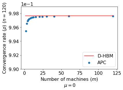
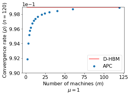
Figure 1: Variation of $\rho_{\text{APC}}$ and $\rho_{\text{HBM}}$ with $m$ for $n=120$ and $\mu\in\{0,1\}$.

Key Inferences

1. APC clearly outperforms D-HBM in both cases. This validates the conclusions drawn from our main results in Section IV.

2. As the number of machines increases, the optimal convergence rate of APC deteriorates and approaches that of D-HBM. This is to be expected for the following reason: as we increase $m$, we increase the number of local data spaces being packed into $\mathbb{R}^{n}$ (the universal data space), possibly reducing the angles between some of the local spaces. This ultimately reduces the cross-machine angular heterogeneity with some positive probability and leads to an increase in the expected value of the upper bound on $\kappa(S)$ established in Theorem 1.

3. APC converges faster when the coefficient mean $\mu$ is increased. This is consistent with the findings of [1] and requires further investigation.

Experiment 2: Dependence of $\rho_{\text{APC}}$ and $\rho_{\text{HBM}}$ on $n$

We retain the setup of Experiment 1, except that we now vary the number of equations (i.e., the size of the matrix $A$) and keep the number of machines fixed, and we now draw the entries of $A$ only from $\mathcal{N}(1,1)$. Note that $\rho_{\text{HBM}}$ depends on the matrix size $n\times n$ via $\kappa(A^{\top}A)$. Therefore, we now expect this convergence rate to vary in our Monte-Carlo simulations. Figure 2 displays the results of Experiment 2 for $m\in\{10,20\}$.

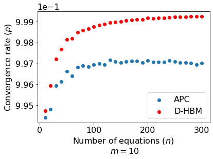
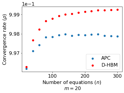
Figure 2: Variation of $\rho_{\text{APC}}$ and $\rho_{\text{HBM}}$ with $n$ for fixed $m$.

Key Inferences

1. Both $\rho_{\text{APC}}$ and $\rho_{\text{HBM}}$ increase with $n$ because the inherent complexity of (1) increases with the number of equations.

2. The convergence rate of APC is remarkably insensitive to $n$ for large values of $n$. This can be explained with the help of Theorems 1 and 2 as follows: we know from Theorem 1 that $\kappa(S)$ is upper-bounded by a quantity that depends on $n$ only through the cross-machine angular heterogeneity $\theta_{\text{H}}$. Given that the rows of $A$ are i.i.d. Gaussian random vectors, we do not expect $\theta_{\text{H}}$ to decrease with $n$, which implies that $\kappa(S)$ (and hence $\rho_{\text{APC}}$) is bounded with respect to $n$.

Experiment 3: Asymptotic behavior of $\theta_{H}$

This experiment uses a different setup. We generate $n$ independent zero-mean random vectors $v_{1},...,v_{n}$, each with covariance matrix $I$. We normalize each of the vectors to obtain $\tilde{v_{i}}:=\frac{v_{i}}{\|v_{i}\|}$, which is a standard way of generating points on $\mathbb{S}^{n-1}$. Next, we compute the empirical mean of $C=\max_{1\leq i<j\leq n}|\langle\tilde{v_{i}},\tilde{v_{j}}\rangle|$ by performing $T=100$ simulations for $n\in[200]$. The results are plotted in Figure 3.

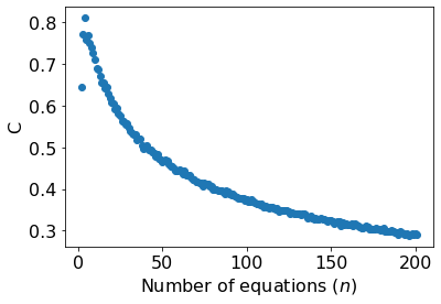
Figure 3: Variation of $C=\max_{1<i<j\leq n}|\langle\tilde{v_{i}},\tilde{v_{j}}\rangle|$ with $n$.

We observe that $C$ approaches $0$ in the limit as $n\to\infty$.

Key Inference

Note that $|\langle\tilde{v_{i}},\tilde{v_{j}}\rangle|\leq C$. Therefore, as $n\rightarrow\infty$, the vectors $\tilde{v_{1}},...,\tilde{v_{n}}$ begin to closely resemble an orthonormal basis for $\mathbb{R}^{n}$. Next, suppose that $\tilde{v}_{1},\ldots,\tilde{v}_{n}$ are the rows of $A$, and consider $\mathcal{R}(A_{i})$ and $\mathcal{R}(A_{j})$ for any $i$ and $j$ in $[m]$ such that $i\neq j$. Asymptotically, a basis of each of these row spaces can be found among $\tilde{v_{1}},...,\tilde{v_{n}}$, with the two bases being disjoint. We can therefore conclude that the inner product of any two vectors, one of which is chosen from $\mathcal{R}(A_{i})$ and the other from $\mathcal{R}(A_{j})$, asymptotically approaches 0, or that $\theta_{\text{H}}\rightarrow\frac{\pi}{2}$ as $n\to\infty$.

VI CONCLUSION AND FUTURE DIRECTIONS

In the context of distributively solving a large-scale system of linear equations, we compared the convergence rates of two classes of algorithms that differ greatly in their design, namely, gradient descent-based methods such as D-HBM, and projection-based methods such as APC. In doing so, we developed a novel, geometric notion of data heterogeneity called angular heterogeneity, and we used it to characterize the convergence rates of a number of distributed linear system solvers belonging to each class. On the basis of our analysis, we not only established the superiority of APC for typical real-world scenarios both theoretically and empirically, but we also provided several interesting insights into the effect of angular heterogeneity on the efficiencies of the studied methods. As a by-product of our investigation, we obtained a tight bound on the condition number of an arbitrary square matrix in terms of the Euclidean norms of its rows and the angles between them.

In the future, we aim to delve deeper into the effect of the number of machines on the convergence rates of projection-based methods such as APC. It would also be instructive to use the condition number bounds derived in this paper to characterize the expected convergence rate of APC in different randomized settings. Other future avenues include the continual/incremental setting as in [23] as well as characterizing the implicit bias of APC in the underdetermined (overparameterized) case [24, 25].

Appendix

VI-A Proof of Theorem 1

Proof.

We perform the steps outlined below Theorem 1.

Step 1

For each $i\in[m]$, let $\tilde{P}_{i}:=I-P_{i}$ denote the orthogonal projector onto $\mathcal{R}(A_{i})$. Using the property [21, Eq. (5.13.4)] of orthogonal projectors, we can show that ${\tilde{P}_{i}=\sum_{j=1}^{p_{i}}v_{j}^{i}(v_{j}^{i})^{\top}}$, where $\{v_{j}^{i}:j\in[p_{i}]\}$ form an orthonormal basis for $\mathcal{R}(A_{i})$. It now follows from (11) that

$$S=\sum_{i=1}^{m}(I-P_{i})=\sum_{i=1}^{m}\tilde{P}_{i}=\sum_{i=1}^{m}\sum_{j=1}^{p_{i}}v_{j}^{i}(v_{j}^{i})^{\top}.$$

Equivalently, $S=VV^{\top}$, where

$$V:=\begin{bmatrix}\uparrow&\uparrow&...&\uparrow&\uparrow&...&\uparrow&...&\uparrow\\ v_{1}^{1}&v_{2}^{1}&...&v_{p_{1}}^{1}&v_{1}^{2}&...&v_{p_{2}}^{2}&...&v_{p_{m}}^{m}\\ \downarrow&\downarrow&...&\downarrow&\downarrow&...&\downarrow&...&\downarrow\end{bmatrix}.$$

It follows that

$$\kappa(S)=\kappa(VV^{\top})\stackrel{{\scriptstyle(a)}}{{=}}\frac{\lambda_{\max}(VV^{\top})}{\lambda_{\min}(VV^{\top})},$$ (24)

where $(a)$ holds because the symmetry of $VV^{\top}$ implies that its eigenvalues equal its singular values. Thus, it suffices to bound the minimum and the maximum eigenvalues of $VV^{\top}$.

Step 2

Since $V$ is a square matrix, we can use the singular value decomposition of $V$ to show that $V^{\top}V$ and $VV^{\top}$ have the same eigenvalues: the squares of the singular values of $V$. Hence, it suffices to bound the eigenvalues of $V^{\top}V$. To this end, we first define

$$V_{i}:=\begin{bmatrix}\uparrow&\uparrow&...&\uparrow\\ v_{1}^{i}&v_{2}^{i}&...&v_{p_{i}}^{i}\\ \downarrow&\downarrow&...&\downarrow\end{bmatrix}$$

so that $V=\begin{bmatrix}V_{1}&\ldots&V_{m}\end{bmatrix}$. Noticing that each $V_{i}$ is orthogonal, we obtain

$$V^{\top}V=\begin{bmatrix}I_{p_{1}\times p_{1}}&V_{1}^{\top}V_{2}&\ldots&V_{1}^{\top}V_{m}\\ V_{2}^{\top}V_{1}&I_{p_{2}\times p_{2}}&\ldots&V_{2}^{\top}V_{m}\\ \vdots&\vdots&\ddots&\vdots\\ V_{m}^{\top}V_{1}&V_{m}^{\top}V_{2}&\ldots&I_{p_{m}\times p_{m}}\end{bmatrix}.$$

It follows that

$$V^{\top}V=I+\begin{bmatrix}O_{p_{1}\times p_{1}}&V_{1}^{\top}V_{2}&\ldots&V_{1}^{\top}V_{m}\\ V_{2}^{\top}V_{1}&O_{p_{2}\times p_{2}}&\ldots&V_{2}^{\top}V_{m}\\ \vdots&\vdots&\ddots&\vdots\\ V_{m}^{\top}V_{1}&V_{m}^{\top}V_{2}&\ldots&O_{p_{m}\times p_{m}}\end{bmatrix}.$$

Let $L$ denote the second summand (i.e., $L:=V^{\top}V-I$), and note that $V^{\top}V,I,L$ are all symmetric. It thus follows from Weyl’s inequality that $\lambda_{\min}(V^{\top}V)\geq\lambda_{\min}(I)+\lambda_{\min}(L).$ As a result,

$$\lambda_{\min}(V^{\top}V)\geq 1+\lambda_{\min}(L)\geq 1-\rho(L).$$ (25)

Similarly,

$$\lambda_{\max}(V^{\top}V)\leq 1+\rho(L).$$ (26)

Step 3

We know from [21, (7.1.12)] that every eigenvalue $\lambda$ of $L$ satisfies $|\lambda|\leq\|L\|_{2}$. On the other hand, by the definition of the operator norm, we have $\|L\|_{2}=\sup_{\|z\|=1}\|Lz\|_{2}$. Now, pick any $z\in\mathbb{R}^{n}$ and partition it as ${z=\begin{bmatrix}z_{1}^{\top}\,\,z_{2}^{\top}\,\,\cdots\,\,z_{m}^{\top}\end{bmatrix}^{\top}}$ where we choose $z_{i}\in\mathbb{R}^{p_{i}}$ for every $i\in[m]$, so that $z$ becomes conformable to block multiplication with $L$. Explicitly performing this block multiplication enables us to observe that

$$\|Lz\|^{2} =\sum_{i=1}^{m}\left\|\sum_{j=1,j\neq i}^{m}(V_{i}^{\top}V_{j})z_{j}\right\|^{2}$$

$$\stackrel{{\scriptstyle(a)}}{{\leq}}\sum_{i=1}^{m}\left(\sum_{j=1,j\neq i}^{m}\|V_{i}^{\top}V_{j}\|\|z_{j}\|\right)^{2},$$

where $(a)$ holds because of Triangle inequality and sub-multiplicativity of matrix norms. This can be expressed compactly as $\|Lz\|^{2}\leq\|L_{\text{com}}\psi_{\text{com}}(z)\|^{2}$, where

$$L_{\text{com}}:=\begin{bmatrix}0&\|V_{1}^{\top}V_{2}\|&\ldots&\|V_{1}^{\top}V_{m}\|\\ \|V_{2}^{\top}V_{1}\|&0&\ldots&\|V_{2}^{\top}V_{m}\|\\ \vdots&\vdots&\ddots&\vdots\\ \|V_{m}^{\top}V_{1}\|&\|V_{m}^{\top}V_{2}\|&\ldots&0\end{bmatrix}$$

and $\psi_{\text{com}}(z):=\begin{bmatrix}\|z_{1}\|\,\,\|z_{2}\|\,\,\cdots\,\,\|z_{m}\|\end{bmatrix}^{\top}.$ Equivalently, ${\|Lz\|\leq\|L_{\text{com}}\psi_{\text{com}}(z)\|}$. Now, note that ${\|\psi_{\text{com}}(z)\|=\|z\|}$, which implies that $\|\psi_{\text{com}}(z)\|=1$ if and only if $\|z\|=1$. Thus,

$$\|L\|=\sup_{\|z\|=1}\|Lz\|\leq\sup_{\|z\|=1}\|L_{\text{com}}\psi_{\text{com}}(z)\|=\|L_{\text{com}}\|.$$ (27)

On the other hand, we also have

$$\|V_{i}^{\top}V_{j}\|=\|V_{i}^{\top}\tilde{P}_{i}^{\top}\tilde{P}_{j}V_{j}\|\leq\|V_{i}^{\top}\|\|\tilde{P}_{i}^{\top}\tilde{P}_{j}\|\|V_{j}^{\top}\|,$$

where the equality is a consequence of $V_{i}=\tilde{P}_{i}V_{i}$, which holds because the columns of $V_{i}$ belong to $\mathcal{R}(A_{i})$ by construction. Next as $V_{i}$ is unitary, we have $\|V_{i}\|_{2}=1$, so which gives

$$\|V_{i}^{\top}V_{j}\|\leq\|\tilde{P}_{i}^{\top}\tilde{P}_{j}\|=\|\tilde{P}_{i}\tilde{P}_{j}\|=\cos(\theta_{ij}),$$

where the second equality follows from [21, Eq. (5.15.2)]. Therefore, $O\leq L_{\text{com}}\leq L_{\text{UB}}$, where

$$L_{\text{UB}}:=\begin{bmatrix}0&\cos\theta_{\text{H}}&\ldots&\cos\theta_{\text{H}}\\ \cos\theta_{\text{H}}&0&\ldots&\cos\theta_{\text{H}}\\ \vdots&\vdots&\ddots&\vdots\\ \cos\theta_{\text{H}}&\cos\theta_{\text{H}}&\ldots&0\end{bmatrix}.$$

We now observe that

$$\rho(L)\stackrel{{\scriptstyle(a)}}{{=}}\|L\|\stackrel{{\scriptstyle(b)}}{{\leq}}\|L_{\text{com}}\| \stackrel{{\scriptstyle(c)}}{{=}}\rho(L_{\text{com}})$$ (28)

$$\stackrel{{\scriptstyle(d)}}{{\leq}}\rho(L_{\text{UB}})$$ (29)

$$\stackrel{{\scriptstyle(e)}}{{\leq}}(m-1)\cos\theta_{\text{H}},$$ (30)

where $(a)$ holds because $L$ is symmetric (which implies that its spectral radius equals its maximum singular value, which in turn equals its Euclidean norm), $(b)$ follows from (27), $(c)$ holds because $L_{\text{com}}$ is symmetric (since $\|V_{i}^{\top}V_{j}\|=\|(V_{i}^{\top}V_{j})^{\top}\|=\|V_{j}^{\top}V_{i}\|$), $(d)$ follows from the inequality $L_{\text{com}}\leq L_{\text{UB}}$ and from [21, Example 7.10.2], and $(e)$ follows from the Gerschgorin circle theorem.

Step 4

Combining (24), (25), (26) and (28) immediately yields the desired bound. ∎

VI-B Proof of Theorem 2

Proof.

We perform the steps outlined below Theorem 2.

Step 1

Observe that

$$\kappa(A^{\top}A) \stackrel{{\scriptstyle(a)}}{{=}}\kappa(AA^{\top})$$

$$=\kappa(R^{\top}Q^{\top}QR)$$

$$\stackrel{{\scriptstyle(b)}}{{=}}\kappa(R^{\top}R)$$

$$\stackrel{{\scriptstyle(c)}}{{=}}(\kappa(R))^{2},$$

where $(a)$ holds because $A^{\top}A$ and $AA^{\top}$ have the same eigenvalues (and by symmetry the same singular values as well), $(b)$ holds because $Q^{\top}Q=I$, which follows from the fact that $Q$ has orthonormal columns by definition, and $(c)$ holds because the singular values of $R^{\top}R$ are the squares of those of $R$.

Similarly, since the singular values of $A^{\top}A$ are the squares of those of $A$, we assert that $\kappa(A^{\top}A)=(\kappa(A))^{2}$. Thus, we have shown that $\kappa(A^{\top}A)=(\kappa(A))^{2}=(\kappa(R))^{2}.$ Since condition numbers are non-negative by definition, this implies that

$$~{}\kappa(A)=\kappa(R).$$ (31)

Step 2

We first sort the columns of $A^{\top}$ (or the rows of $A$) in the descending order of their norms. Note that re-ordering the columns of $A^{\top}$ is equivalent to right-multiplying $A^{\top}$ by a permutation matrix $P\in\mathbb{R}^{n\times n}$. So, we choose $P$ in such a way that the $k$-th column $\tilde{a}_{k}$ of the column-sorted matrix $\tilde{A}^{\top}:=A^{\top}P$ satisfies $\left\lVert\tilde{a}_{k}\right\rVert\geq\left\lVert\tilde{a}_{\ell}\right\rVert$ for all $\ell\geq k$. We now let $\tilde{A}^{\top}=\tilde{Q}\tilde{R}$ denote the $QR$ decomposition of $\tilde{A}^{\top}$ and observe that

$$\kappa(A^{\top}A) \stackrel{{\scriptstyle(a)}}{{=}}\kappa(A^{\top}PP^{\top}A)$$ (32)

$$=\kappa(\tilde{A}^{\top}\tilde{A})$$ (33)

$$\stackrel{{\scriptstyle(b)}}{{=}}\kappa(\tilde{A}\tilde{A}^{\top})$$ (34)

$$=\kappa(\tilde{R}^{\top}\tilde{Q}^{\top}\tilde{Q}\tilde{R})$$ (35)

$$\stackrel{{\scriptstyle(c)}}{{=}}\kappa(\tilde{R}^{\top}\tilde{R})$$ (36)

$$\stackrel{{\scriptstyle(d)}}{{=}}(\kappa(\tilde{R}))^{2},$$ (37)

where $(a)$ holds because $P$ being a permutation implies $PP^{\top}=I$, $(b)$ holds because $\tilde{A}^{\top}\tilde{A}$ and $\tilde{A}\tilde{A}^{\top}$ have the same eigenvalues (and by symmetry the same singular values as well), $(c)$ holds because $\tilde{Q}^{\top}\tilde{Q}=I$, which follows from the fact that $\tilde{Q}$ has orthonormal columns by definition, and $(d)$ holds because the singular values of $\tilde{R}^{\top}\tilde{R}$ are the squares of those of $\tilde{R}$. We now relabel $\tilde{Q}$ and $\tilde{R}$ as $Q$ and $R$, respectively, for ease of notation.

Next, let $\rho(\cdot)$ denote the spectral radius of a square matrix, and observe that

$$\kappa(R) \stackrel{{\scriptstyle(a)}}{{=}}\left\lVert R\right\rVert\left\lVert R^{-1}\right\rVert$$ (38)

$$\stackrel{{\scriptstyle(b)}}{{\geq}}\rho(R)\rho(R^{-1})$$ (39)

$$=\frac{\rho(R)}{\lambda_{\min}(R)}\stackrel{{\scriptstyle(c)}}{{=}}\frac{\max_{k\in[n]}|r_{kk}|}{\min_{k\in[n]}|r_{kk}|},$$ (40)

where $(a)$ follows from a standard definition of the condition number of a matrix [21], $(b)$ holds because any matrix norm of a given square matrix serves as an upper bound on its spectral radius [21], and $(c)$ holds because $R$ being triangular implies that its eigenvalues are equal to its diagonal entries $\{r_{kk}\}_{k=1}^{n}$. These diagonal entries are given by Gram-Schmidt orthogonalization [21] as

$$r_{11}=\left\lVert\tilde{a}_{1}\right\rVert,\text{ }r_{kk}=\left\|\tilde{a}_{k}-\sum_{s=1}^{k-1}(q_{s}^{\top}\tilde{a}_{k})q_{s}\right\|\text{ for }k>1,$$ (41)

where $q_{s}$ denotes the $s$-th column of $Q$ for $s\in[n]$. .

Step 3

To bound the above expression in terms of $\left\lVert\tilde{a}_{k}\right\rVert$ and $\theta_{\min}^{(k)}$, observe first that

$$r_{kk}^{2} \stackrel{{\scriptstyle(a)}}{{=}}\left\lVert\tilde{a}_{k}\right\rVert^{2}-\left\lVert\sum_{s=1}^{k-1}(q_{s}^{\top}\tilde{a}_{k})q_{s}\right\rVert^{2}\stackrel{{\scriptstyle(b)}}{{=}}\left\lVert\tilde{a}_{k}\right\rVert^{2}-\sum_{s=1}^{k-1}(q_{s}^{\top}\tilde{a}_{k})^{2},$$ (42)

where $(a)$ follows from the orthogonality of $\sum_{s=1}^{k-1}(q_{s}^{\top}\tilde{a}_{k})q_{s}$ and $\tilde{a}_{k}-\sum_{s=1}^{k-1}(q_{s}^{\top}\tilde{a}_{k})q_{s}$ and $(b)$ follows from the fact that $\{q_{s}\}_{s=1}^{n}$ are orthonormal. Therefore, it is sufficient to bound $\sum_{s=1}^{k-1}(q_{s}^{\top}\tilde{a}_{k})$ in terms of the angles between $\tilde{a}_{k}$ and other columns of $\tilde{A}^{\top}$ (which form a subset of the rows of $A$). To this end, choose

$$\ell^{*}:=\operatorname*{arg\,max}_{1\leq\ell\leq k}\left(\frac{|\tilde{a}_{\ell}^{\top}\tilde{a}_{k}|}{\left\lVert\tilde{a}_{\ell}\right\rVert\left\lVert\tilde{a}_{k}\right\rVert}\right)$$

as the row index that minimizes the angle between $\tilde{a}_{\ell}$ and $\tilde{a}_{k}$ for $1\leq\ell\leq k$, use $\tilde{\theta}_{\min}^{(1:k)}:=\cos^{-1}\left(\frac{|\tilde{a}_{\ell^{*}}^{\top}\tilde{a}_{k}|}{\left\lVert\tilde{a}_{\ell^{*}}\right\rVert\left\lVert\tilde{a}_{k}\right\rVert}\right)$ to denote this minimum angle, and observe that

$$\left\lVert\tilde{a}_{k}\right\rVert\left\lVert\tilde{a}_{\ell^{*}}\right\rVert\cos\tilde{\theta}_{\min}^{(1:k)}$$

$$=\tilde{a}_{k}^{\top}\tilde{a}_{\ell^{*}}$$

$$=\tilde{a}_{k}^{\top}QQ^{\top}\tilde{a}_{\ell^{*}}$$

$$\stackrel{{\scriptstyle(a)}}{{=}}\left(Q^{-1}\tilde{a}_{k}\right)^{\top}\left(Q^{-1}\tilde{a}_{\ell^{*}}\right)$$

$$\stackrel{{\scriptstyle(b)}}{{=}}\sum_{s=1}^{n}\left(q_{s}^{\top}\tilde{a}_{k}\right)\left(q_{s}^{\top}\tilde{a}_{\ell^{*}}\right)$$

$$\stackrel{{\scriptstyle(c)}}{{\leq}}\left(\sum_{s=1}^{n}\left(q_{s}^{\top}\tilde{a}_{k}\right)^{2}\right)^{\frac{1}{2}}\left(\sum_{t=1}^{n}\left(q_{t}^{\top}\tilde{a}_{\ell^{*}}\right)^{2}\right)^{\frac{1}{2}}$$

$$\stackrel{{\scriptstyle(d)}}{{=}}\left(\sum_{s=1}^{n}\left(q_{s}^{\top}\tilde{a}_{k}\right)^{2}\right)^{\frac{1}{2}}\left\lVert\tilde{a}_{\ell^{*}}\right\rVert,$$

where $(a)$ holds because $Q$ being an orthogonal matrix implies $Q^{\top}=Q^{-1}$, $(b)$ and $(d)$ hold because $Q^{-1}\tilde{a}_{k}$ and $Q^{-1}\tilde{a}_{\ell^{*}}$ are, respectively, the $k$-th and the $\ell^{*}$-th columns of $Q^{-1}\tilde{A}=R$, whose entries, respectively, are $\{q_{s}^{\top}\tilde{a}_{k}\}_{s=1}^{n}$ and $\{q_{s}^{\top}\tilde{a}_{\ell^{*}}\}_{s=1}^{n}$ (not all of which are non-zero), and $(c)$ follows from Cauchy-Schwarz inequality. Dividing throughout by $\left\lVert\tilde{a}_{\ell^{*}}\right\rVert$ now yields

$$\sum_{s=1}^{n}\left(q_{s}^{\top}\tilde{a}_{k}\right)^{2}\geq\left\lVert\tilde{a}_{k}\right\rVert^{2}\cos^{2}\tilde{\theta}_{\min}^{(1:k)}.$$ (43)

Since we have $q_{s}^{\top}\tilde{a}_{k}=0$ for all $s\geq k$ by Gram-Schmidt orthogonalization, combining (42) and (43) culminates in

$$r_{kk}^{2}\leq\left\lVert\tilde{a}_{k}\right\rVert^{2}-\left\lVert\tilde{a}_{k}\right\rVert^{2}\cos^{2}\tilde{\theta}_{\min}^{1:k}=\left\lVert\tilde{a}_{k}\right\rVert^{2}\sin^{2}\theta_{\min}^{(1:k)}.$$

Hence,

$$\min_{k\in[n]}r_{kk}\leq\min_{k\in[n]}\left\{\left\lVert\tilde{a}_{k}\right\rVert\sin\theta_{\min}^{(1:k)}\right\}.$$ (44)

We now consider (44) and replace $\theta_{\min}^{(1:k)}$, which is the minimum angle between $\tilde{a}_{k}$ and any of $\{\tilde{a}_{s}:1\leq s<k\}$, with

$$\tilde{\theta}_{\min}^{(k)}:=\cos^{-1}\max_{\ell\in[n]}\left(\frac{|\tilde{a}_{k}^{\top}\tilde{a}_{\ell}|}{\left\lVert\tilde{a}_{k}\right\rVert\left\lVert\tilde{a}_{\ell}\right\rVert}\right),$$

which is the minimum angle between $\tilde{a}_{k}$ and any other row of $A$. This is possible for the following reasons: for the index $\ell_{*}:=\operatorname*{arg\,max}_{\ell\in[n]\setminus\{k\}}\left(\frac{|\tilde{a}_{k}^{\top}\tilde{a}_{\ell}|}{\left\lVert\tilde{a}_{k}\right\rVert\left\lVert\tilde{a}_{\ell}\right\rVert}\right)$, we either have $\ell_{*}<k$ or $k<\ell_{*}\leq n$. In the former case, we have $\tilde{\theta}_{\min}^{(1:k)}=\tilde{\theta}_{\min}^{(k)}$, whereas in the latter case we have

$$\tilde{\theta}_{\min}^{(1:k)}>\tilde{\theta}_{\min}^{(k)}=\cos^{-1}\left(\frac{|\tilde{a}_{k}^{\top}\tilde{a}_{\ell_{*}}|}{\left\lVert\tilde{a}_{k}\right\rVert\left\lVert\tilde{a}_{\ell_{*}}\right\rVert}\right)\geq\tilde{\theta}_{\min}^{(1:\ell_{*})}$$

as well as $\left\lVert\tilde{a}_{k}\right\rVert\geq\left\lVert\tilde{a}_{\ell_{*}}\right\rVert$ because of the way we have sorted the rows of $\tilde{A}$. In either case, we have

$$\min\left\{\left\lVert\tilde{a}_{\ell_{*}}\right\rVert\sin\tilde{\theta}_{\min}^{(1:\ell_{*})},\left\lVert\tilde{a}_{k}\right\rVert\sin\tilde{\theta}_{\min}^{(1:k)}\right\}\leq\left\lVert\tilde{a}_{k}\right\rVert\sin\tilde{\theta}_{\min}^{(k)}.$$

In light of (44), this means $\min_{k}r_{kk}\leq\min_{k}\left\lVert\tilde{a}_{k}\right\rVert\sin\tilde{\theta}_{\min}^{(k)}$. Since $\{\tilde{a}_{k}:k\in[n]\}=\{a_{k}:k\in[n]\}$, it follows that $\{\tilde{\theta}_{\min}^{(k)}:k\in[n]\}=\{\theta_{\min}^{(k)}:k\in[n]\}$, and hence,

$$~{}\min_{k\in[n]}r_{kk}\leq\min_{k\in[n]}\left\{\left\lVert a_{k}\right\rVert\sin\theta_{\min}^{(k)}\right\}.$$ (45)

Step 4

Finally, we observe that:

$$~{}\kappa(R) \stackrel{{\scriptstyle(a)}}{{\geq}}\frac{r_{11}}{\min_{k\in[n]}r_{kk}}\stackrel{{\scriptstyle(b)}}{{\geq}}\frac{\left\lVert\tilde{a}_{1}\right\rVert}{\min_{k\in[n]}\left\{\left\lVert\tilde{a}_{k}\right\rVert\sin\theta_{\min}^{(k)}\right\}}$$ (46)

$$\stackrel{{\scriptstyle(c)}}{{=}}\frac{\max_{k\in[n]}\left\lVert a_{k}\right\rVert}{\min_{\ell\in[n]}\left\{\left\lVert a_{\ell}\right\rVert\sin\theta_{\min}^{(\ell)}\right\}},$$ (47)

where $(a)$ follows from (38) and the non-negativity of $\{r_{kk}\}_{k=1}^{n}$, $(b)$ follows from (41) and (45), and $(c)$ is a result of the way $\tilde{A}$ sorts the rows of $A$ (see Step 1). Invoking (31) now yields the desired lower bound. ∎

References

- [1] N. Azizan, F. Lahouti, A. S. Avestimehr, and B. Hassibi, “Distributed solution of large-scale linear systems via Accelerated Projection-Based Consensus,” IEEE Transactions on Signal Processing, vol. 67, no. 14, pp. 3806–3817, 2019.
- [2] C. K. Ko¸, A. Güvenç, and B. Bakkalo LU, “Exact solution of linear equations on distributed-memory multiprocessors,” Parallel Algorithm and Applications, vol. 3, no. 1-2, pp. 135–143, 1994.
- [3] L. Xiao, S. Boyd, and S. Lall, “A scheme for robust distributed sensor fusion based on average consensus,” in IPSN 2005. Fourth International Symposium on Information Processing in Sensor Networks, 2005., pp. 63–70, IEEE, 2005.
- [4] N. Santoro, Design and analysis of distributed algorithms. John Wiley & Sons, 2006.
- [5] J. Verbraeken, M. Wolting, J. Katzy, J. Kloppenburg, T. Verbelen, and J. S. Rellermeyer, “A survey on distributed machine learning,” ACM Computing Surveys (CSUR), vol. 53, no. 2, pp. 1–33, 2020.
- [6] Y. Xiao, N. Zhang, W. Lou, and Y. T. Hou, “A survey of distributed consensus protocols for blockchain networks,” IEEE Communications Surveys & Tutorials, vol. 22, no. 2, pp. 1432–1465, 2020.
- [7] M. Zinkevich, M. Weimer, L. Li, and A. Smola, “Parallelized stochastic gradient descent,” Advances in Neural Information Processing Systems, vol. 23, 2010.
- [8] B. Recht, C. Re, S. Wright, and F. Niu, “Hogwild!: A lock-free approach to parallelizing stochastic gradient descent,” Advances in Neural Information Processing Systems, vol. 24, 2011.
- [9] K. Yuan, Q. Ling, and W. Yin, “On the convergence of decentralized gradient descent,” SIAM Journal on Optimization, vol. 26, no. 3, pp. 1835–1854, 2016.
- [10] Y. E. Nesterov, “A method of solving a convex programming problem with convergence rate O(k2),” in Doklady Akademii Nauk, vol. 269, pp. 543–547, Russian Academy of Sciences, 1983.
- [11] B. T. Polyak, “Some methods of speeding up the convergence of iteration methods,” USSR Computational Mathematics and Mathematical Physics, vol. 4, no. 5, pp. 1–17, 1964.
- [12] K. Chakrabarti, N. Gupta, and N. Chopra, “Robustness of Iteratively Pre-conditioned Gradient-Descent Method: The case of distributed linear regression problem,” in 2021 American Control Conference (ACC), pp. 2248–2253, IEEE, 2021.
- [13] S. Boyd, N. Parikh, E. Chu, B. Peleato, J. Eckstein, et al., “Distributed optimization and statistical learning via the Alternating Direction Method of Multipliers,” Foundations and Trends® in Machine learning, vol. 3, no. 1, pp. 1–122, 2011.
- [14] I. S. Duff, R. Guivarch, D. Ruiz, and M. Zenadi, “The augmented Block Cimmino distributed method,” SIAM Journal on Scientific Computing, vol. 37, no. 3, pp. A1248–A1269, 2015.
- [15] F. Sloboda, “A projection method of the Cimmino type for linear algebraic systems,” Parallel Computing, vol. 17, no. 4-5, pp. 435–442, 1991.
- [16] M. Arioli, I. Duff, J. Noailles, and D. Ruiz, “A block projection method for sparse matrices,” SIAM Journal on Scientific and Statistical Computing, vol. 13, no. 1, pp. 47–70, 1992.
- [17] S. Karczmarz, “Angenaherte auflosung von systemen linearer glei-chungen,” Bull. Int. Acad. Pol. Sic. Let., Cl. Sci. Math. Nat., pp. 355–357, 1937.
- [18] S. S. Alaviani and N. Elia, “A distributed algorithm for solving linear algebraic equations over random networks,” IEEE Transactions on Automatic Control, vol. 66, no. 5, pp. 2399–2406, 2020.
- [19] Y. Huang, Z. Meng, and J. Sun, “Scalable distributed least square algorithms for large-scale linear equations via an optimization approach,” Automatica, vol. 146, p. 110572, 2022.
- [20] S. Mou, J. Liu, and A. S. Morse, “A distributed algorithm for solving a linear algebraic equation,” IEEE Transactions on Automatic Control, vol. 60, no. 11, pp. 2863–2878, 2015.
- [21] C. D. Meyer, Matrix analysis and applied linear algebra, vol. 71. Siam, 2000.
- [22] L. Lessard, B. Recht, and A. Packard, “Analysis and design of optimization algorithms via integral quadratic constraints,” SIAM Journal on Optimization, vol. 26, no. 1, pp. 57–95, 2016.
- [23] Y. Min, K. Ahn, and N. Azizan, “One-pass learning via bridging orthogonal gradient descent and recursive least-squares,” in 2022 IEEE 61st Conference on Decision and Control (CDC), pp. 4720–4725, 2022.
- [24] N. Azizan and B. Hassibi, “Stochastic gradient/mirror descent: Minimax optimality and implicit regularization,” in International Conference on Learning Representations, 2019.
- [25] N. Azizan, S. Lale, and B. Hassibi, “Stochastic mirror descent on overparameterized nonlinear models,” IEEE Transactions on Neural Networks and Learning Systems, 2021.