The quality of school track assignment decisions by teachers

Abstract

We study the quality of secondary school track assignment decisions in the Netherlands, using a regression discontinuity design. In 6th grade, primary school teachers assign each student to a secondary school track. If a student scores above a track-specific cutoff on the standardized end-of-primary education test, the teacher can upwardly revise this assignment. By comparing students just left and right of these cutoffs, we find that between 50-90% of the students are trapped in track: these students are on the high track after four years, only if they started on the high track in first year. The remaining (minority of) students are always low: they are always on the low track after four years, independently of where they started. These proportions hold for students near the cutoffs that shift from the low to the high track in first year by scoring above the cutoff. Hence, for a majority of these students the initial (unrevised) track assignment decision is too low. The results replicate across most of the secondary school tracks, from the vocational to the academic tracks, and stand out against an education system with a lot of upward and downward track mobility.

Keywords: Ability tracking, Student allocation, Regression discontinuity design
JEL: D81, I24, C26

1 Introduction

Countries differ widely in the nature and degree of ability tracking in education. Tracking can be efficient as teachers can target instruction closer to the needs of students. Theoretically, therefore, both high and low achievers might benefit from some level of ability tracking. Benefits of ability tracking have also been documented empirically (e.g. Duflo et al. (2011); Kwak and Lee (2023)). However, if assignment errors are important and if there are limited opportunities to resolve these errors, any (individual or societal) benefits from tracking might be outweighed by its costs. Costs from assignment errors might arise from, among others, a mismatch between a student’s potential and the level of instruction, stigmatization and/or unfavorable peer group dynamics.

In this paper we study the quality of the secondary school track assignment process in the Netherlands, where students are assigned to different educational programs at the age of 12. The assignment of primary students to secondary school tracks is based primarily on the primary school teacher’s track assignment decision. This decision is binding and secondary schools are not (as a rule) permitted to deviate from this (WVO, 2014). Teachers can inform their decisions with student performance on standardized achievement tests throughout primary school as well as, potentially, with other (observed) skills and behaviors. The task of combining this information is obviously challenging and errors in the assignment process seem almost inevitable. In Dutch, the primary school teacher’s track assignment decision is known as the schooladvies, which translates as track recommendation. In this paper we will use the terms track assignment decision and track recommendation interchangeably.

To date it remains largely unclear to what extent primary school teachers make correct assignment decisions, and, whether any potential errors have consequences in the longer term. In this paper we study the quality of the teacher assignment decisions in conjunction with an analysis of the flexibility of the education system. In particular we study the extent to which primary school teachers make mistakes in the assignment of students to secondary school tracks and whether these mistakes (if any) have consequences for track enrollment in the first four years of secondary education.

An analysis of the quality of track assignment decisions is challenging. The main reason is that we do not observe students’ secondary school outcomes under track assignment decisions that have not been made. Ideally, we want to compare outcomes between the actual assignment decision to potential outcomes of alternative assignment decisions. In this paper we consider two potential outcomes: fourth-year secondary school enrollment while having started on a relatively high and a relatively low track.

A comparison of these two potential outcomes enables us to make a distinction between four exhaustive and mutually exclusive types of students: (i) Always High students are always on the high track after four years of secondary education, independently of first year enrollment, (ii) Always Low students are always on the low track after four years, independently of first year enrollment, (iii) Trapped in Track students are on the low track after four years if they start on the low track, but on the high track after four years if they start on the high track, and (iv) Slow Starters who are on the low track after four years if they start on the high track, but on the low track after four years if they start on the high track. If we would observe each student’s type and the actual teachers’ assignment decision, we could evaluate whether teachers make mistakes, and whether these mistakes have consequences in the longer term.

In this paper we combine detailed administrative data on the educational careers of all primary school students in the Netherlands with a Regression Discontinuity Design (RDD) to mimic the setting described above. The Dutch secondary school system has five educational tracks, from lower pre-vocational to a university preparatory track, roughly reflecting population quintiles in educational achievement. In 6th grade, the primary school teacher formulates the track assignment decision in March of the school year, where each student is assigned to one of the five secondary school tracks. Mixed track assignments are also possible.

In April or May of the school year, the 6th grade students take the standardized end-of-primary education test. The test scores also map into a track level, based on nationwide and predetermined test score cutoffs. We refer to the mapping of the test score to a track level as the test-based track recommendation. If the test-based recommendation, is higher than the teacher’s track recommendation recorded in March, the teacher is mandated by law to consider an upwards revision of the track recommendation (WPO, 2014). Therefore, if students score above certain test score cutoffs, the student may receive an upgraded track recommendation and subsequently enroll on a higher track in the first year of secondary education. The possibility of track assignment revision was introduced in the school year 2014/15 to provide an extra opportunity for students with high achievement scores, relative to their initial (unrevised) track recommendation.

We compare students with the same initial track recommendation near the relevant test score cutoffs, and use a score just above the cutoff as an instrumental variable for first-year track enrollment to estimate the causal effect of first-year on fourth-year track enrollment. This effect is estimated for compliers: students who start secondary education in first year on the high track, because they scored above the test score cutoff. Using the logic of Abadie (2002), we use the expressions for the untreated and treated complier means to find four expressions that can generally be used to bound the four types of students defined above. In specific cases, however, the proportion of each of the student types can be point identified. Our results meet the conditions for these specific cases most of the times.

We show that students near the cutoffs have similar background characteristics and that the density of the number of students is continuous near the test score cutoffs. This supports the continuity assumption that students just to the left and right of the cutoffs have similar potential outcomes. Additionally, since we apply the logic of Abadie (2002) to binary outcome variables, our final treatment effects of interest correspond to the specification test of the instrumental variable (IV) assumptions developed by Kitagawa (2015). The intuition is that, under the IV assumptions, all our treatment effects identify proportions of students, and can therefore not be negative. Across all our results, we do not find one statistically significant negative treatment effect.

Our main result is that a majority (between 50-90%) of the complier students are of the Trapped in Track type. This means that for a majority of the complier students, the initial assignment is too low and that the system provides insufficient opportunities for upward mobility. We find that the remaining minority of the complier students are Always Low. For them the initial assignment was appropriate, but the revised high-track assignment has no consequences for enrollment after four years of secondary education. We find no strong evidence for the existence of complier students that are of the Always High or Slow Starter type. We find qualitatively similar results across almost the full range of initial track assignment decisions. In particular, results for students with initial assignments for the pre-vocational tracks are similar to the results for students with initial assignments for the more academically oriented tracks.

Our study complements recent studies who investigate the role of early tracking in secondary education by exploiting age at primary school entry cutoffs, which induces variation in track enrollment (Dustmann et al., 2017; Oosterbeek et al., 2021). These studies show that students who are old-for-grade are more likely to enroll in higher tracks than students who are young-for-grade. Both find that these initial enrollment effects disappear with time, due to built-in flexibilities of the system. While these studies indicate that the German and Dutch system are flexible enough to offset some of the initial differences in enrollment, they cannot address the quality of the teachers’ assignment decisions. The reason is that the differential assignment of the young-for-grade and the old-for-grade may be correct (or incorrect) for both groups. Because in our analysis only the track assignment itself is as-good-as randomly assigned, our approach allows for an assessment of the relative quality of the assignments. This has clear policy implications as there are various costs associated with mistakes in the assignments.

Most directly, there are costs of paying teachers. A commonly used way for upward track mobility in the Netherlands is the “stacking of diplomas”. After graduating from one track, students might enroll in the next (higher) track. In this process, students typically spend an extra year in school. The extra one year in school costs roughly €10,000 per case. In addition, these students would enter the labor market one year later, which reduces life-time income and tax payments (e.g. Oosterbeek et al. (2021)). In this draft we follow students until the fourth year of secondary school. In subsequent drafts, we will extend the time horizon beyond these four years, towards graduation and the transition into tertiary education or work.

A more subtle cost might emerge when mistakes in track assignments weakens the connection between the level and pace of instruction and a student’s potential. Students might miss out on a critical period in their cognitive development (Hoxby, 2021). This might have longer term consequences, personally (e.g. frustration) and financially. In the current draft, we do not report on results for the development of cognitive skills. In subsequent drafts, however, we will report on two such outcomes. First, we will present results on the standardized secondary school math test (the rekentoets), which is comparable for students in the different vocational tracks. Second, we will report on the effect of secondary school major choice (profielen). It seems plausible that the Trapped in Track students who enroll in the high track find the curriculum more challenging. This might influence their choice of major. The major choice, however, may also be affected for the Always High and Always Low type for which assignment has no longer term effects on enrollment.

The rest of the paper is organized as follows. In Section 2 we discuss some relevant aspects of the Dutch education system. In Section 3 we introduce the four student types and our argument for identification. Section 4 introduces the data and Section 5 describes the RD specification and estimation. In Section 6 we present our main results on the quality of the track recommendations. Section 7 concludes and discusses future updates to our analysis and separate ongoing research projects.

2 Empirical setting

In the Netherlands, the transition from primary to secondary school happens at the end of the 6th grade, when students are approximately 12 year old. As students enter secondary education in grade 7, they are tracked into one of five different educational tracks. There are three preparatory vocational tracks, which prepare for tertiary vocational education. From more to less vocational there are the vmbo-bl, vmbo-kl and the vmbo-gt tracks. In addition there are two more academically oriented tracks, which are the college preparatory track (havo) and the university preparatory track (vwo). Hybrid tracks (or “bridge” tracks, in Dutch brugklassen) which effectively combine different tracks are also common. These hybrid tracks typically delay track assignment by one or two years. The secondary school tracks provide access to different levels of further education. The academically most demanding vwo track provides direct access to almost all university programs offered by Dutch universities. The vocational tracks allow for direct access to tertiary vocational programs.

The system of educational tracking in the Netherlands has existed for generations. In the 1960s there was a major overhaul of the system, with the intention to make it more meritocratic. During various stages of modernization, a number of features were built in to ensure the meritocratic working of the system. For example, standardized achievement testing was introduced in the 1970s to inform assignment decisions. Also, the new system allowed for upward and downward track mobility to fix any remaining mistakes in the assignment process.

For many years, the secondary school track placement has been based primarily on the primary school’s 6th grade teacher’s assignment decision. The teachers can inform their decision with student performance on standardized tests throughout primary school and the decision can, in part, be based on subjective judgments of other skills and behaviors. The task of assigning students to tracks involves a prediction of a student’s potential in the short and medium term, based on imperfect information.

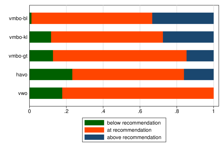
Figure 1: Secondary school enrollment, four years after starting secondary education.

Notes: The figure is based on almost all students that took the end-of-primary Cito test in the 6th grade of primary school in the school years 2014/15, 2015/16 and 2016/17. See Section 4 for details on the construction of our sample.

In Figure 1 we plot the distribution of track enrollments after four years of secondary education, separately for five track assignment decisions. In particular, we show the fraction of students that is enrolled at a track level below, at, or above the primary teacher’s track assignment decision. Figure 1 shows that track mobility is indeed quite common. For example, about 20% of students assigned to havo reach the higher vwo track four years later, while another 20% of them drops down a level to vmbo-gt. Track mobility in the first few years of secondary education seems often facilitated by the existence of the hybrid tracks we mentioned above. The upward and downward mobility that is observed in the data might suggest some misallocation of students to tracks. It also suggests, however, that at least some of these mistakes (if any) are sorted out rather quickly by the facilitation of track mobility.

2.1 The possibility of track assignment revision

Starting in the school year 2014/15, the regulations of the track assignment process were changed in two ways. First, the primary school teacher’s recommendation became binding for track placement in secondary education (WVO, 2014). Secondary schools were not (as a rule) permitted to place students on a track level above the recommended level. Second, an option was introduced for the teacher to upwardly revise the track recommendation. After the teacher recommendation was recorded in March, all students would take the standardized end-of-primary education test in April or May. The scores on this test also map into track levels, based on nationwide and predetermined test score cutoffs. We refer to the mapping of a test score to a track level as the test-based track recommendation. If the test-based recommendation, is higher than the teacher’s track recommendation recorded in March, the teacher is mandated by law to consider an upwards revision of the “initial” track recommendation (WPO, 2014). An actual revision of the initial assignment is only optional and dependent, again, on the teacher’s judgment.

Table LABEL:tab:toetsadvies of Appendix D presents the mapping of the test scores to the track levels for the cohorts we study in this paper. It shows that, for example, in 2014/15 test scores between 537 and 544 correspond to a havo test-based recommendation. Then, for example, students who are initially assigned to vmbo-gt by the teacher, and obtain a test score of 537 or higher, qualify for a track assignment revision. For these students a score of 537 is a relevant test score cutoff: scoring at or above 537 may result in a track assignment revision and a higher track enrollment in first year of secondary education.

3 Framework

3.1 The four student types and misallocation

Consider that there are two tracks: track High ($H$) and track Low ($L$). Let $H_{t}$ be a dummy variable that is equal to one if the student is enrolled on the high track, and zero if a student is enrolled on the low track, in year $t$ of secondary education. Throughout the paper, we suppress the student index for notational convenience. Define potential fourth-year track enrollment as $H_{4}(H_{1})$. That is, for each student there are two potential outcomes. $H_{4}(1)$ is track enrollment in year four, when starting secondary education on the high track in year one. $H_{4}(0)$ is track enrollment in year four when starting secondary education on the low track in year one. Based on these two potential outcomes, we can categorize students into four exhaustive and mutually exclusive student types:

1. Always High ($\mathrm{AH}$): $\{H_{4}(1)=H_{4}(0)=1\}$.

2. Always Low ($\mathrm{AL}$): $\{H_{4}(1)=H_{4}(0)=0\}$.

3. Trapped in Track ($\mathrm{TT}$): $\{H_{4}(1)-H_{4}(0)=1\}$.

4. Slow Starters ($\mathrm{SS}$): $\{H_{4}(1)-H_{4}(0)=-1\}$.

Type Always High ($\mathrm{AH}$) students are always on the high track after four years of secondary education, regardless of where they start in the first year. In contrast, type Always Low ($\mathrm{AL}$) students are always on the low track in year four, regardless of where they start in year one. Type Trapped in Track ($\mathrm{TT}$) students are enrolled on the high (low) track after four years only when they start secondary education on the high (low) track. Type Slow Starters ($\mathrm{SS}$) are enrolled on the high (low) track after four years of secondary education when starting on the low (high) track.

For type $\mathrm{AH}$ and $\mathrm{AL}$ the starting track has no consequences for track enrollment in year four, whereas for type $\mathrm{TT}$ and $\mathrm{SS}$ the starting track is consequential. Type $\mathrm{TT}$ strictly benefit from being assigned to the high track, whereas type $\mathrm{SS}$ strictly benefit from being assigned to the low track. We stipulate that students aim to be enrolled in the highest track possible by year four, and that they rather be enrolled in this highest possible track sooner than later. This allows us to define two types of track assignments that are incorrect:

Definition 1 (Two types of incorrect track assignments).

Incorrect track assignment with longer term enrollment effects. For type $\mathrm{TT}$ and $\mathrm{SS}$ students, incorrect assignment to the low and high track respectively has longer term consequences for track enrollment.
Incorrect track assignment without longer term enrollment effects. For type $\mathrm{AH}$ and $\mathrm{AL}$ students, incorrect assignment to the low and high track respectively does not have longer term consequences for track enrollment.

We use terms like incorrect assignments, wrong assignments, and misallocation interchangeably.

3.2 Interpreting observed mobility

Table 1 describes, for all four student types, the observed mobility when assigned to the low and the high track. We use the red (orange) color to indicate misallocations with (without) longer term consequences on track enrollment. The table shows that observed patterns of mobility cannot, in general, be clearly characterized. In particular, there are always two possible types that can explain a single observed pattern of mobility. It follows that we can give Figure 1 a best-case and a worst-case interpretation. For students assigned to the low track, the observed upward mobility may be type $\mathrm{SS}$ students (best-case) or type $\mathrm{AH}$ students (worst-case), and the observed immobility may reflect type $\mathrm{AL}$ students (best-case) or type $\mathrm{TT}$ students (worst-case).

Note that in our framework, for students assigned to the high track, the observed immobility never reflects misallocation and the observed downward mobility always reflects misallocation. In the best-case (worst-case) interpretation, however, the downward mobility reflects type $\mathrm{AL}$ ($\mathrm{SS}$) students. This shows that the observed mobility in Figure 1 does not allow us to conclude anything definitive about the quality of the teachers’ assignments, nor on whether the system is sufficiently flexible to resolve any of these potential assignment errors within the first four years of secondary education.

Table 1: When is each student type misallocated and observed mobility

Assigned to low track	Observed mobility	Assigned to high track	Observed mobility
$\mathrm{AH}$	Upward	$\mathrm{AH}$	Immobility
$\mathrm{AL}$	Immobility	$\mathrm{AL}$	Downward
$\mathrm{TT}$	Immobility	$\mathrm{TT}$	Immobility
$\mathrm{SS}$	Upward	$\mathrm{SS}$	Downward

• Notes. Misallocations with longer term enrollment effects are indicated in red. Misallocations without longer term enrollment effects are indicated in orange.

Table 1 also helps in realizing how difficult the track assignment problem can be, particularly considering the uncertainty about student abilities. If a teacher is not sure whether a student is type $\mathrm{AL}$ or $\mathrm{TT}$, she might risk assigning this student to the high track. This would be a “low-regret” option: a type $\mathrm{AL}$ student would drop down to the low track, while the assignment to the high track is crucial for type $\mathrm{TT}$ students. However, when a teacher is unsure whether a student is type $\mathrm{TT}$ or $\mathrm{SS}$, a low-regret option is not available. The government recommendation for teachers to “assign high, when in doubt” (which is broadly perceived as a no-regret option) is harmful for type $\mathrm{SS}$ students.

In Appendix E we develop a simple deterministic model of human capital development in the context of ability tracking. A key characteristic of this model is that achievement and potential (e.g. innate ability) are not necessarily perfectly aligned. Based on this model we can rationalize the existence of the four types of students. The model predicts that type $\mathrm{SS}$ students have high ability, but (relatively) low initial achievement that does not match their high ability. These students initially benefit from instruction at a lower level, matching their initial level of achievement. As they progress, their high ability allows them to catch up, which implies upward mobility. In contrast, if type $\mathrm{SS}$ students are misallocated to the high track in the first year of secondary education, they struggle since the pace of instruction does not match their low initial level of achievement. In this case, the model would predict downward mobility.

The model rationalizes type $\mathrm{TT}$ as students with relatively high levels of initial achievement and somewhat more modest levels of ability. If these students are correctly assigned to the high track in the first year of secondary education, their high levels of initial achievement are enough to benefit from the level of instruction on the high track as to not drop down a level. On the other hand, if they are misallocated to the low track, the type $\mathrm{TT}$ students do not have enough ability to compensate for the lower level of instruction on the low track. This prevents them from moving up to the high track track. The type $\mathrm{TT}$ students are therefore always immobile, regardless of whether they are assigned to the high or low track.

3.3 Identifying the four types of students

We only observe one potential outcome for each student. That is, we either observe $H_{4}(1)$ or $H_{4}(0)$. Given this fundamental problem, how do we identify the relative presence of each student type?

For each student with a teacher track recommendation $T$, teachers have to consider an upwards revision if scores on the end-of-primary education test suggest a higher track recommendation than $T$ (as discussed in Section 2.1). Because the test-based recommendations are based on nationwide and predetermined test score cutoffs $c_{T}$, we can use a fuzzy Regression Discontinuity Design (RDD). Let the variable $Z$ be determined by the test score $S$ lying on either side of a cutoff $c_{T}$ as follows,

$$Z=\left\{\begin{array}[]{ll}0&S<c_{T},\\ 1&S\geq c_{T}.\end{array}\right.$$ (3)

We will refer to $Z$ as the treatment assignment variable, where students with $Z=1$ are “treated” with a teacher that considers an upwards revision of the initial track assignment.

We generalize the potential outcome framework introduced in Section 3.1 to include the treatment assignment variable $Z$. Define $H_{1}(Z)$ as potential first-year track enrollment for each $Z$, and $H_{4}(Z,H_{1})$ as potential fourth-year track enrollment for each combination of $Z$ and $H_{1}$. Our fuzzy RD with $H_{1}$ as endogenous treatment variable and $H_{4}$ as outcome variable requires the standard fuzzy RD assumptions.

Assumption 1 (Standard fuzzy RD assumptions).

1. (Continuity) $H_{4}(z,h_{1}),H_{1}(z)$ are continuous in $s$ at $s=c_{T}$ for all $z,h_{1}$.

2. (Exclusion restriction) $H_{4}(z,h_{1})=H_{4}(h_{1})$ for all $z,h_{1}$.

3. (First stage) $\underset{s\to^{+}c_{T}}{\lim}\mathbb{E}[H_{1}|S=s]>\underset{s\to^{-}c_{T}}{\lim}\mathbb{E}[H_{1}|S=s]$.

4. (Monotonicity) $H_{1}(1)\geq H_{1}(0)$ for each student.

Assumption 1a requires that students just to the left and right of the test score cutoffs are similar. Assumption 1b imposes that scoring above the cutoff only has an effect on fourth-year track enrollment if it also affects first-year track enrollment. Note that 1b ensures that the potential outcomes for $H_{4}$ are again identical as introduced in Section 3.1. Assumption 1c requires that scoring above the cutoff has a positive effect on first-year track enrollment. Assumption 1d subsequently assumes that, for each student, this effect cannot be negative.

Similar to the four student types based on how $H_{4}$ responds to $H_{1}$, there are also four types based on how $H_{1}$ responds to $Z$. In the treatment literature, these groups are commonly referred to as Always Takers ($\mathrm{AT}:\{H_{1}(1)=H_{1}(0)=1\}$), Never Takers ($\mathrm{NT}:\{H_{1}(1)=H_{1}(0)=0\}$), Compliers ($\mathrm{C}:\{H_{1}(1)-H_{1}(0)=1\}$), and Defiers ($\mathrm{D:\{H_{1}(1)-H_{1}(0)=-1\}}$). Assumption 1d ensures that defiers do not exist. Compliers are the students that shift from the low track to the high track in first year when they score above the cutoff. Then Proposition 1 shows that the four following fuzzy RD estimands each identify the proportion of two different student types, for the complier students that have a test score at the cutoff.

Proposition 1 (Four fuzzy RD estimands).

Under 1, it holds that:

$$\frac{\underset{s\to^{+}c_{T}}{\lim}\mathbb{E}[H_{4}\times H_{1}|S=s]-\underset{s\to^{-}c_{T}}{\lim}\mathbb{E}[H_{4}\times H_{1}|S=s]}{\underset{s\to^{+}c_{T}}{\lim}\mathbb{E}[H_{1}|S=s]-\underset{s\to^{-}c_{T}}{\lim}\mathbb{E}[H_{1}|S=s]}= \,\mathbb{P}[\mathrm{AH}|\mathrm{C},S=c_{T}]+\mathbb{P}[\mathrm{TT}|\mathrm{C},S=c_{T}],$$ (4)

$$\frac{\underset{s\to^{+}c_{T}}{\lim}\mathbb{E}[H_{4}\times L_{1}|S=s]-\underset{s\to^{-}c_{T}}{\lim}\mathbb{E}[H_{4}\times L_{1}|S=s]}{\underset{s\to^{+}c_{T}}{\lim}\mathbb{E}[L_{1}|S=s]-\underset{s\to^{-}c_{T}}{\lim}\mathbb{E}[L_{1}|S=s]}= \,\mathbb{P}[\mathrm{AH}|\mathrm{C},S=c_{T}]+\mathbb{P}[\mathrm{SS}|\mathrm{C},S=c_{T}],$$ (5)

$$\frac{\underset{s\to^{+}c_{T}}{\lim}\mathbb{E}[L_{4}\times H_{1}|S=s]-\underset{s\to^{-}c_{T}}{\lim}\mathbb{E}[L_{4}\times H_{1}|S=s]}{\underset{s\to^{+}c_{T}}{\lim}\mathbb{E}[H_{1}|S=s]-\underset{s\to^{-}c_{T}}{\lim}\mathbb{E}[H_{1}|S=s]}= \,\mathbb{P}[\mathrm{AL}|\mathrm{C},S=c_{T}]+\mathbb{P}[\mathrm{SS}|\mathrm{C},S=c_{T}],$$ (6)

$$\frac{\underset{s\to^{+}c_{T}}{\lim}\mathbb{E}[L_{4}\times L_{1}|S=s]-\underset{s\to^{-}c_{T}}{\lim}\mathbb{E}[L_{4}\times L_{1}|S=s]}{\underset{s\to^{+}c_{T}}{\lim}\mathbb{E}[L_{1}|S=s]-\underset{s\to^{-}c_{T}}{\lim}\mathbb{E}[L_{1}|S=s]}= \,\mathbb{P}[\mathrm{AL}|\mathrm{C},S=c_{T}]+\mathbb{P}[\mathrm{TT}|\mathrm{C},S=c_{T}],$$ (7)

where $L_{1}=(1-H_{1})$ and $L_{4}=(1-H_{4})$.

The proof is shown in Appendix A.

The results in Proposition 1 are not new. In particular, (4) and (5) reflect Equations (3) and (4) from Abadie (2002), and the numerators of (4) and (5) correspond to Equation (1.1) from Kitagawa (2015). Abadie (2002) uses that, in an IV framework, the treated and the untreated complier means can be estimated by using as outcome variable in reduced form regressions the original outcome variable ($H_{4}$) multiplied by, respectively, a treatment dummy ($H_{1}$) and control dummy ($1-H_{1}$). Since our outcome variable ($H_{4}$) is binary, the treated and untreated complier means reflect probabilities. This, in turn, is used by Kitagawa (2015) to develop a specification test for the joint validity of the IV assumptions 1a-d. The intuition behind this test is that, since (4) and (5) reflect probabilities under 1, their empirical counterparts should be bigger than zero.

The equations (4)-(7) represent a system of equations that, in general, can be used to construct bounds on the proportion of each student type. However, a particularly informative case might arise when one of the equations is zero, which would immediately set the proportion of two student types to zero. In that case, the two other proportions can be point identified. Note also that the sum of (4)-(7) is equal to two since the proportion of each student type appears twice across the four equations.

4 Data

We use proprietary administrative data from Statistics Netherlands on all students that take the standardized end-of-primary education test in the 6th grade of primary school in the school years 2014/15, 2015/16, and 2016/17. We refer to these three different groups of students as cohorts. The 2014/15 cohort is the first that is affected by the new track assignment regulations discussed in Section 2.1. We follow these three cohorts for four years into secondary education, and so the 2016/17 cohort is the last that we consider.

For almost all students we observe the initial (unrevised) teacher track recommendation, the scores on the standardized end-of-primary education test, and the final track recommendation. The final recommendation might differ from the initial recommendation in case of an upwards revision. For all of these students, we also observe track enrollment in the first four years of secondary education. We also observe several relevant background characteristics, including gender, age, and household income.

There are two criteria that we use to construct our final sample. First, our final sample only contains students from primary schools that use the end-of-primary education test provided by test developer Cito. While Cito is still by far the largest provider of this test, other test developers have more recently entered the market for end-of-primary education testing. Second, we select the students who start secondary education in the year after they are assigned. That is, for students who repeat the 6th grade of primary school, we use the last observed enrollment in grade 6.

4.1 Constructing $H_{1}$ and $H_{4}$

The variables $H_{1}$ and $H_{4}$ are constructed as follows. For students with a “single” track recommendation (i.e. a recommendation for one specific track, which are vmbo-bl, vmbo-kl, vmbo-gt, havo and vwo), $H_{1}=1$ if first-year track enrollment is strictly above the level of the recommendation, and $H_{1}=0$ otherwise. For example, for students with a vmbo-gt recommendation, $H_{1}=1$ if they start in first year on the havo track or higher, and $H_{1}=0$ otherwise.

The variable $H_{4}$ is constructed similarly, but is based on track enrollment after four years of secondary education. We ignore the possibility of a grade repetition. That is, students might be enrolled on the high track after four years, but may have repeated a year and are therefore only in third grade. Grade repetition in the first four years of secondary education however is uncommon, with roughly 90% of the students showing normal grade progressions in the first four years of secondary education. Moreover, in Section 6 we find that this percentage does not vary discontinuously at the test score cutoffs.

For students with a “mixed” track recommendation (i.e. vmbo-bl/vmbo-kl, vmbo-kl/vmbo-gt, vmbo-gt/havo or havo/vwo) the construction of the variables is slightly different. The variable $H_{1}$ equals one if the student is enrolled on a track level that is strictly above the lowest track of the mixed recommendation and $H_{1}$ equals zero otherwise. For example, for students with a havo/vwo recommendation, $H_{1}=1$ if they are enrolled in first year in vwo, and $H_{1}=0$ otherwise. The variable $H_{4}$ is, again, constructed similarly.

4.2 Descriptive statistics

Table 4.2 presents some descriptive statistics for our final estimation sample. Column 1 shows the number of students with a specific initial (unrevised) track recommendation. The column shows that the single track recommendations are the most common, although some mixed recommendations are also reasonably common. Note that our final sample does not include the students with the single vwo track recommendation, since this highest recommendation can never be upwardly revised.

5.3 Binarized treatment variables

We binarize multivalued first-year track enrollment into our treatment variable of interest ($H_{1}$). As discussed by Angrist and Imbens (1995); Andresen and Huber (2021), binarization of the treatment variable may lead to violations of the exclusion restriction assumption 1c. These violations might arise if (i) scoring above the cutoff (i.e. the instrument $Z$) affects the underlying multivalued treatment within support areas above and below the binarization threshold and (ii) such instrument-induced changes in the multivalued treatment affect fourth-year track enrollment.

Although it is difficult to completely rule out that the binarization generates violations of the exclusion restriction, we note that our treatment effects of interest are used by Kitagawa (2015) to develop a specification test for the joint validity of the IV assumptions 1a-d. The intuition behind this test is that, since (4) and (5) reflect probabilities under 1, their empirical counterparts should be bigger than zero. In Section 6 we indeed do not estimate treatment effects that are statistically significantly smaller than zero or bigger than one. We interpret this result as first evidence in support of the exclusion restriction. In future drafts we will report upon additional specification tests in the spirit of Kitagawa (2015).

To measure the presence of misallocation of students to tracks, we are interested in comparing similar students who enroll in different tracks in first year of secondary education. In our setting, we have found evidence that a test score above the cutoff affects first-year enrollment in (at least) two ways. Using the specification test introduced by Kitagawa (2015) we have clearly rejected the assumptions for an IV approach that aims to estimate the causal effect of a revised teacher recommendation on enrollment. We interpret this finding as a violation of the exclusion restriction for that IV approach: test scores above the cutoff are also used directly by secondary schools to make first-year track placement decisions. While this is not in complete accordance with the new regulations presented in WVO (2014), it may be motivated by the need to create (more or less) equally sized classes. Because high schools cannot fully control student enrollment, they sometimes face inconvenient distributions of teachers’ recommendations.

6 Results

Table LABEL:tab:fresults1 presents the 2SLS estimates for (8). The four columns correspond to the four different second stage outcome variables, where the five rows correspond to the five initial track recommendations with a large and highly statistically significant first stage documented in Table LABEL:tab:fs.

Under the IV assumptions 1a-d, the second stage parameters should be bounded between zero and one. In Table LABEL:tab:fresults1 we find that, while some estimates are smaller than zero or bigger than one, these deviations are not statistically significant. Based on this result we cannot reject the IV assumptions and the interpretation that is implied by Proposition 1.

& vwo 15,950 0.52*** 0.36** 0.48*** 0.64*** (0.10) (0.16) (0.07) (0.16)

vmbo-gt havo 28,817 0.51*** -0.12 0.49*** 1.12*** (0.11) (0.27) (0.10) (0.29)

vmbo-gt/havo havo 12,832 0.98*** -0.19 0.02 1.19*** (0.22) (0.34) (0.18) (0.37)

vmbo-kl vmbo-gt 17,223 0.92*** -0.24 0.08 1.24*** (0.12) (0.18) (0.07) (0.21)

• Notes. ***, **, * refers to statistical significance at the 1, 5, and 10% level. Robust standard errors in parentheses. The second stage of the fuzzy RD in (8) uses a polynomial of order one, that is allowed to differ on each side of the cutoff, and a bandwidth of three test score points. The standard errors are approximated by dividing the robust standard errors of the reduced form by the first stage estimate.

One of the key empirical results is that for four out of the five initial track recommendations (i.e. havo, vmbo-gt, vmbo-gt/havo, and vmbo-kl) the estimates in column 3 are reasonably small and not significantly different from zero. In other words, except for the initial track recommendation havo/vwo in row two, we cannot reject that the sum of the fraction of the Always High type and the fraction of the Slow Starter type among the compliers is zero. If we proceed on the basis of this result, we are able to rule out the presence of these two types, and the estimates presented in column 2 and 4 reflect, respectively, the fraction of Trapped in Track and Always Low among the compliers. Our results therefore suggest that for four of the five initial track recommendations the compliers are either Trapped in Track or Always Low. We also find that the estimated fractions of the Trapped in Track type is always higher than the fraction of the Always Low type. This is true in particular for compliers who are initially assigned to vmbo-gt/havo or to vmbo-kl. For these two track recommendations, the compliers seem exclusively of the Trapped in Track type.

The results thus suggest that for a majority of the compliers the initial (unrevised) track assignment is too low. For these students, the low assignment also has consequences for track enrollment in the first four years of secondary education: Trapped in Track students do not reach the high track without being placed on the high track from the start. For the minority of the compliers the initial (unrevised) track assignment was appropriate and the revised assignment was too high. However, for the Always Low type, wrong assignment to the high track has no consequences for track enrollment after four years.

In Table LABEL:tab:nominal2 of Appendix C we show estimates of RD models that use dummy variables for normal grade progression across years as outcome variables. We find that grade repetition increases with time (to about 10% in year four), but we do not find any discontinuity in grade progression at the cutoffs. This result suggest, for example, that the Trapped in Track type who start secondary education on the high track, are not more likely to repeat a grade.

The result presented in Table LABEL:tab:fresults1 for the initial recommendation havo/vwo are less straightforward to interpret. As the estimates in all the columns are sizable and statistically significant, we cannot impose assumptions informed by our results that allow us to point identify the fraction of each student type. In this case, however, the results may be used to provide bounds on those fractions. For example, the estimate in column 5 is significantly smaller than one. As the estimates in column 5 correspond to the sum of the fraction Always Low and the fraction Trapped in Track, the composition of the complier population for this track recommendation is, in some sense, fundamentally different than for the other recommendations.

It is important to realize that the population of students around these cutoffs are students with a test score that is high, relative to the initial track recommendation. We show that the fraction of compliers among these students are mostly of the Trapped in Track type. The high score of these students already may reflect that these students are capable of more than what the initial (unrevised) teacher recommendation would suggest. It is not clear whether teachers had the opportunities to see this potential, or whether they think that high scores on tests are not always meaningful. In future updates of this paper we plan to investigate these issues.

7 Conclusion

In this paper we study the quality of secondary school track assignment decisions by primary school teachers. In the Netherlands, students are assigned to secondary school tracks at the age of 12. The primary school teacher’s assignment decision is binding in the placement of students to tracks in the first year of secondary education. Mistakes in these track assignment decisions can be costly. We present first causal evidence of the quality of these assignment decisions, using a fuzzy RDD.

When students score above a track-specific cutoff on the standardized end-of-primary education test, the teacher can upwardly revise the assignment decision and the student may start secondary education on a higher track. By comparing students just left and right of these cutoffs, we find that between 50-90% of the students are Trapped in Track: these students are on the high track after four years, only if they started on the high track in first year. The remaining (minority of) students are Always Low: they are always on the low track after four years, independently of where they started in first year. This result indicates that the initial (unrevised) assignment decisions of primary school teachers are often too low.

The results presented in this paper specifically apply to compliers with test scores at the cutoffs. Compliers are students who start secondary education on the high track, because they scored above the test score cutoff. These cutoffs are at relatively high levels in the conditional test score distribution. Students with test scores around these cutoffs, therefore, are students with high scores relative to other students who are initially (prior to any revision) assigned to the same track.

Because the initial assignment decisions appear to be too low, we think it is relevant to study the drivers of these assignment decisions. Why are teachers making these mistakes? In future drafts of this paper we plan to study the inputs for the assignment decisions in an effort to answer this question. For example, we will look at the track assignment decisions in conjunction with administrative data on the standardized achievement tests that are administered bi-annually from the primary school grades 1 to 5 (leerlingvolgsysteem). These test scores may feed into the track assignment decisions of teachers. To date, however, it is not clear how teachers weigh or combine this information.

In future versions of this paper we also plan to incorporate some other additions. First, we will extend the time horizon beyond the first four years of secondary education. Second, we will try to investigate outcomes that correlate with cognitive and non-cognitive ability. In particular, we will analyze the effects on the secondary education math test (rekentoets) and on secondary school choice of major (profielen). Third, we plan to investigate the role of hybrid tracks (brugklassen) in facilitating track mobility. Fourth, we will extend our specification tests in the spirit of Kitagawa (2015) to test for violations of the exclusion restriction that we maintain in our analysis.

In separate ongoing research projects we also study other effects of the allocation process that are not necessarily directly reflected in educational outcomes. For example, we are studying the effects of the assignment to different tracks on criminal behavior.

Appendix A Proof Proposition 1

We link observed outcomes to potential outcomes as follows,

$$H_{1}= H_{1}(0)(1-Z)+H_{1}(1)Z,$$ (11)

$$H_{4}= H_{4}(0)(1-H_{1})+H_{4}(1)H_{1},$$ (12)

where (12) uses Assumption 1b.

We can write the denominator of (4) and (6) as,

$$\underset{s\to^{+}c_{T}}{\lim}\mathbb{E}[H_{1}|S=s]-\underset{s\to^{-}c_{T}}{\lim}\mathbb{E}[H_{1}|S=s]$$ (13)

$$= \underset{s\to^{+}c_{T}}{\lim}\mathbb{E}[H_{1}(1)|S=s]-\underset{s\to^{-}c_{T}}{\lim}\mathbb{E}[H_{1}(0)|S=s]$$

$$= \mathbb{E}[H_{1}(1)|S=c_{T}]-\mathbb{E}[H_{1}(0)|S=c_{T}]$$

$$= \mathbb{E}[H_{1}(1)-H_{1}(0)|S=c_{T}]$$

$$= \mathbb{P}[\mathrm{C}|S=c_{T}],$$

where we substitute for potential outcomes from (11), and use Assumption 1a and 1d respectively. Since $L_{1}=(1-H_{1})$, the denominator for (5) and (7) follow immediately,

$$\underset{s\to^{+}c_{T}}{\lim}\mathbb{E}[(1-H_{1})|S=s]-\underset{s\to^{-}c_{T}}{\lim}\mathbb{E}[(1-H_{1})|S=s]$$ (14)

$$= -\big{(}\underset{s\to^{+}c_{T}}{\lim}\mathbb{E}[H_{1}|S=s]-\underset{s\to^{-}c_{T}}{\lim}\mathbb{E}[H_{1}|S=s]\big{)}$$

$$= -\mathbb{P}[\mathrm{C}|S=c_{T}]$$

For the numerators, we use (12) to write

$$H_{4}\times H_{1}= H_{4}(1)H_{1},$$ (15)

$$H_{4}\times(1-H_{1})= H_{4}(0)(1-H_{1}),$$ (16)

$$(1-H_{4})\times H_{1}= (1-H_{4}(1))H_{1},$$ (17)

$$(1-H_{4})\times(1-H_{1})= (1-H_{4}(0))(1-H_{1}).$$ (18)

We can express the numerator of (4) as,

$$\underset{s\to^{+}c_{T}}{\lim}\mathbb{E}[H_{4}\times H_{1}|S=s]-\underset{s\to^{-}c_{T}}{\lim}\mathbb{E}[H_{4}\times H_{1}|S=s]$$ (19)

$$= \underset{s\to^{+}c_{T}}{\lim}\mathbb{E}[H_{4}(1)\times H_{1}(1)|S=s]-\underset{s\to^{-}c_{T}}{\lim}\mathbb{E}[H_{4}(1)\times H_{1}(0)|S=s]$$

$$= \mathbb{E}[H_{4}(1)\times H_{1}(1)|S=c_{T}]-\mathbb{E}[H_{4}(1)\times H_{1}(0)|S=c_{T}]$$

$$= \mathbb{E}[H_{4}(1)\times(H_{1}(1)-H_{1}(0))|S=c_{T}]$$

$$= \mathbb{E}[H_{4}(1)|\mathrm{C},S=c_{T}]\mathbb{P}[\mathrm{C}|S=c_{T}]$$

$$= \mathbb{P}[H_{4}(1)=1|\mathrm{C},S=c_{T}]\mathbb{P}[\mathrm{C}|S=c_{T}]$$

$$= \mathbb{P}[\mathrm{AH}|\mathrm{C},S=c_{T}]\mathbb{P}[\mathrm{C}|S=c_{T}]+\mathbb{P}[\mathrm{TT}|\mathrm{C},S=c_{T}]\mathbb{P}[\mathrm{C}|S=c_{T}],$$

where we substitute for potential outcomes from (15), and use Assumption 1a and 1d respectively. The proof for the numerators of (5), (6), and (7) use the same strategy. For the numerator of (5),

$$\underset{s\to^{+}c_{T}}{\lim}\mathbb{E}[H_{4}\times(1-H_{1})|S=s]-\underset{s\to^{-}c_{T}}{\lim}\mathbb{E}[H_{4}\times(1-H_{1})|S=s]$$ (20)

$$= \underset{s\to^{+}c_{T}}{\lim}\mathbb{E}[H_{4}(0)\times(1-H_{1}(1))|S=s]-\underset{s\to^{-}c_{T}}{\lim}\mathbb{E}[H_{4}(0)\times(1-H_{1}(0))|S=s]$$

$$= \mathbb{E}[H_{4}(0)\times(1-H_{1}(1))|S=c_{T}]-\mathbb{E}[H_{4}(0)\times(1-H_{1}(0))|S=c_{T}]$$

$$= -\mathbb{E}[H_{4}(0)\times(H_{1}(1)-H_{1}(0))|S=c_{T}]$$

$$= -\mathbb{E}[H_{4}(0)|\mathrm{C},S=c_{T}]\mathbb{P}[\mathrm{C}|S=c_{T}]$$

$$= -\mathbb{P}[H_{4}(0)=1|\mathrm{C},S=c_{T}]\mathbb{P}[\mathrm{C}|S=c_{T}]$$

$$= -\mathbb{P}[\mathrm{AH}|\mathrm{C},S=c_{T}]\mathbb{P}[\mathrm{C}|S=c_{T}]-\mathbb{P}[\mathrm{SS}|\mathrm{C},S=c_{T}]\mathbb{P}[\mathrm{C}|S=c_{T}],$$

for the numerator of (6),

$$\underset{s\to^{+}c_{T}}{\lim}\mathbb{E}[(1-H_{4})\times H_{1}|S=s]-\underset{s\to^{-}c_{T}}{\lim}\mathbb{E}[(1-H_{4})\times H_{1}|S=s]$$ (21)

$$= \underset{s\to^{+}c_{T}}{\lim}\mathbb{E}[(1-H_{4}(1))\times H_{1}(1)|S=s]-\underset{s\to^{-}c_{T}}{\lim}\mathbb{E}[(1-H_{4}(1))\times H_{1}(0)|S=s]$$

$$= \mathbb{E}[(1-H_{4}(1))\times H_{1}(1)|S=c_{T}]-\mathbb{E}[(1-H_{4}(1))\times H_{1}(0)|S=c_{T}]$$

$$= \mathbb{E}[(1-H_{4}(1))\times(H_{1}(1)-H_{1}(0))|S=c_{T}]$$

$$= \mathbb{E}[(1-H_{4}(1))|\mathrm{C},S=c_{T}]\mathbb{P}[\mathrm{C}|S=c_{T}]$$

$$= \mathbb{P}[(1-H_{4}(1))=1|\mathrm{C},S=c_{T}]\mathbb{P}[\mathrm{C}|S=c_{T}]$$

$$= \mathbb{P}[\mathrm{AL}|\mathrm{C},S=c_{T}]\mathbb{P}[\mathrm{C}|S=c_{T}]+\mathbb{P}[\mathrm{SS}|\mathrm{C},S=c_{T}]\mathbb{P}[\mathrm{C}|S=c_{T}],$$

and for the numerator of (7),

$$\underset{s\to^{+}c_{T}}{\lim}\mathbb{E}[(1-H_{4})\times(1-H_{1})|S=s]-\underset{s\to^{-}c_{T}}{\lim}\mathbb{E}[(1-H_{4})\times(1-H_{1})|S=s]$$ (22)

$$= \underset{s\to^{+}c_{T}}{\lim}\mathbb{E}[(1-H_{4}(0))\times(1-H_{1}(1))|S=s]-\underset{s\to^{-}c_{T}}{\lim}\mathbb{E}[(1-H_{4}(0))\times(1-H_{1}(0))|S=s]$$

$$= \mathbb{E}[(1-H_{4}(0))\times(1-H_{1}(1))|S=c_{T}]-\mathbb{E}[(1-H_{4}(0))\times(1-H_{1}(0))|S=c_{T}]$$

$$= -\mathbb{E}[(1-H_{4}(0))\times(H_{1}(1)-H_{1}(0))|S=c_{T}]$$

$$= -\mathbb{E}[(1-H_{4}(0))|\mathrm{C},S=c_{T}]\mathbb{P}[\mathrm{C}|S=c_{T}]$$

$$= -\mathbb{P}[(1-H_{4}(0))=1|\mathrm{C},S=c_{T}]\mathbb{P}[\mathrm{C}|S=c_{T}]$$

$$= -\mathbb{P}[\mathrm{AL}|\mathrm{C},S=c_{T}]\mathbb{P}[\mathrm{C}|S=c_{T}]-\mathbb{P}[\mathrm{TT}|\mathrm{C},S=c_{T}]\mathbb{P}[\mathrm{C}|S=c_{T}].$$

Assumption 1c ensures that (4)-(7) are finite.

Appendix B Balancing tests

& vwo -0.01 373 -0.01 -0.02* (0.02) (2,866) (0.01) (0.01) 0.52*** 106,859*** 11.71*** 0.18*** (0.01) (2,393) (0.01) (0.01)

vmbo-gt havo -0.01 2,378 -0.00 -0.00 (0.01) (1,529) (0.01) (0.01) 0.53*** 83,781*** 11.83*** 0.19*** (0.01) (1,184) (0.01) (0.01)

vmbo-gt/havo havo -0.01 -2,369 -0.00 0.00 (0.02) (3,090) (0.02) (0.02) 0.55*** 94,961*** 11.80*** 0.22*** (0.02) (2,611) (0.01) (0.01)

• Notes. This table continues on the next page.

& vmbo-gt -0.04 465 -0.00 0.02 (0.03) (2,965) (0.03) (0.03) 0.57*** 79,342*** 11.90*** 0.19*** (0.03) (2,587) (0.03) (0.02)

vmbo-bl vmbo-kl 0.02 -432 -0.03 -0.02 (0.03) (2,759) (0.03) (0.03) 0.49*** 65,350*** 12.13*** 0.29*** (0.02) (2,299) (0.03) (0.02)

vmbo-bl/vmbo-kl vmbo-kl 0.01 -5,538 -0.01 0.03 (0.04) (4,948) (0.04) (0.03) 0.53*** 74,843*** 12.01*** 0.25*** (0.03) (4,594) (0.03) (0.03)

• Notes. ***, **, * indicate statistical significance at the 1, 5 and 10% level. Robust standard errors in parentheses. The (reduced-form) equation in (10) uses a polynomial of order one, that is allowed to differ on each side of the cutoff, and a bandwidth of three test score points. We report the RD estimates $\hat{\gamma}_{X}$ (top) and the means just left of the cutoff $\hat{\psi}_{X}$ (bottom).

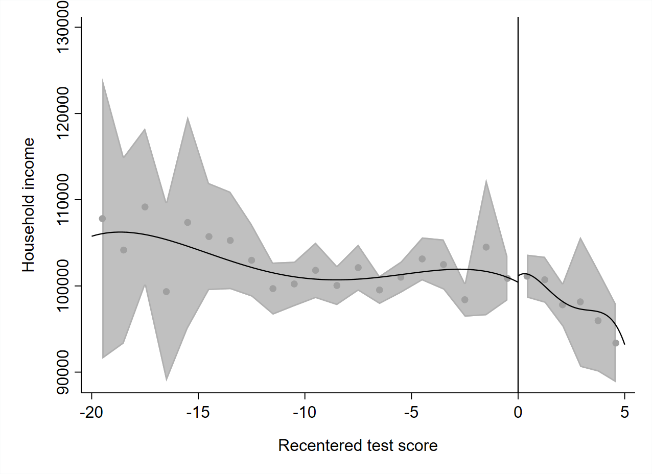
Figure 3: Visual representation of balancing tests for household income

Notes: Test scores are centered at the relevant cutoffs. From left to right, and top to bottom, for each figure the initial track recommendation is: havo, havo/vwo, vmbo-gt, vmbo-gt/havo, vmbo-kl, vmbo-kl/vmbo-gt, vmbo-bl, vmbo-bl/vmbo-kl.

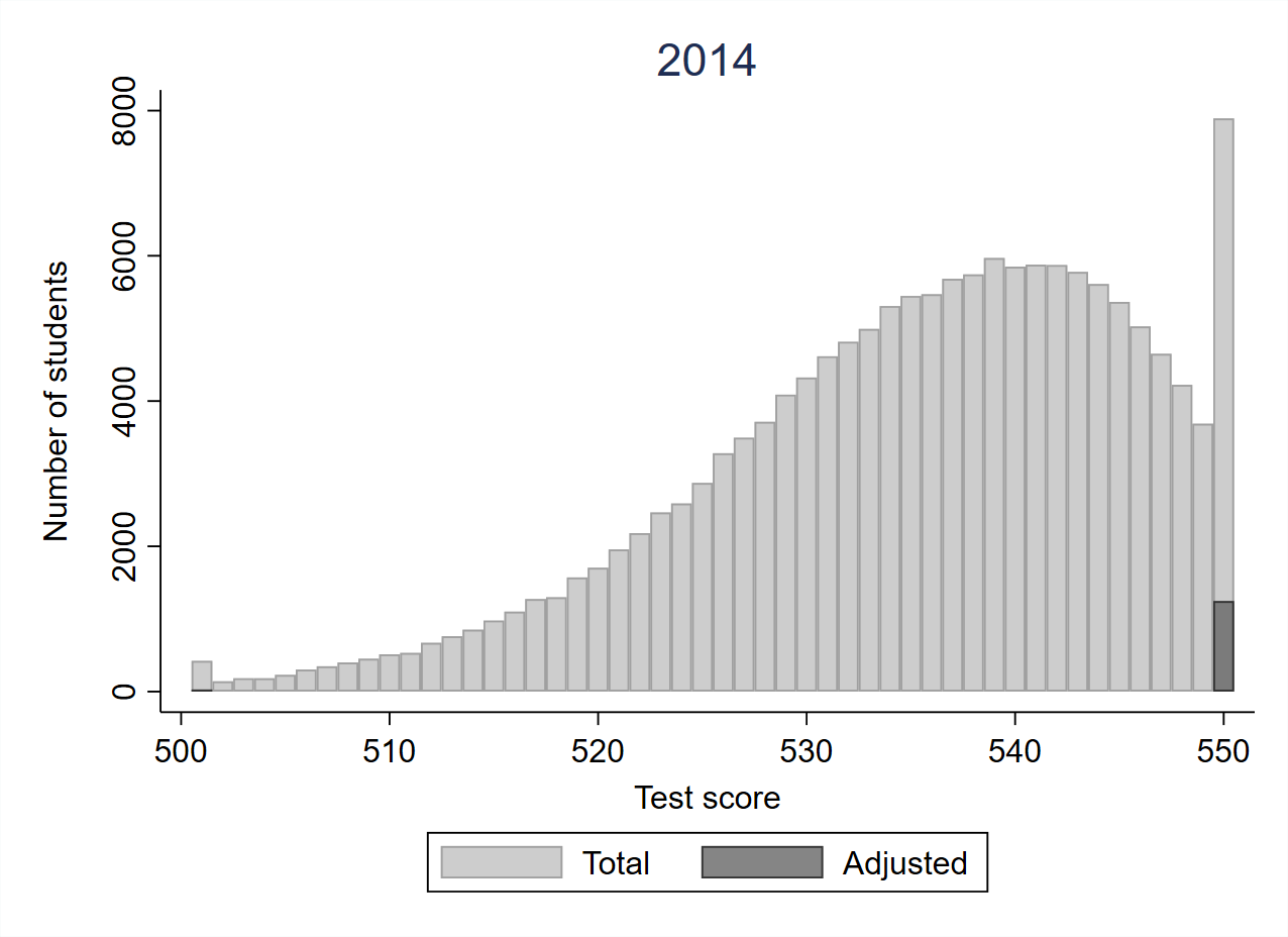
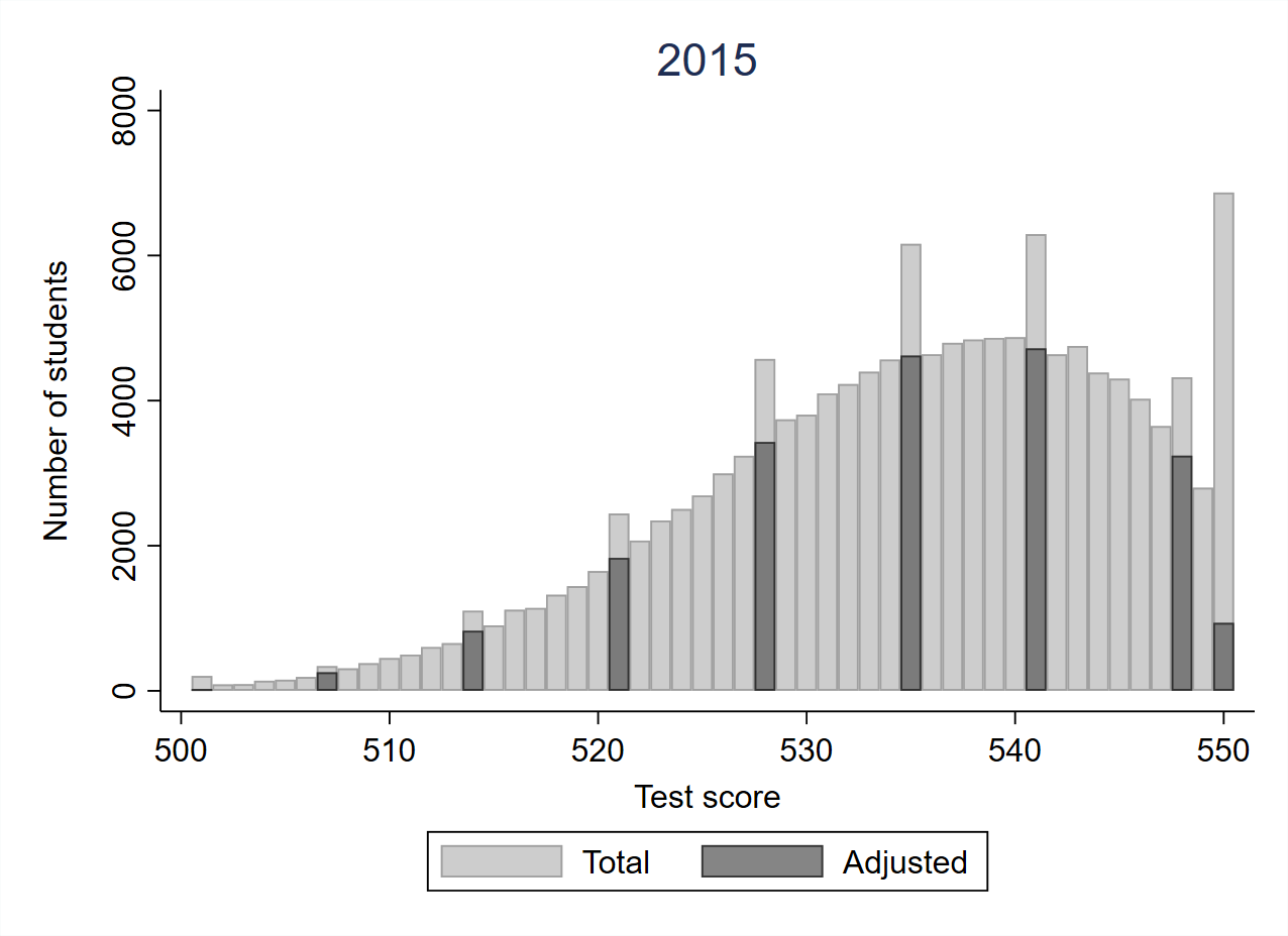
Figure 4: Test score distribution per cohort

Notes: This figure plots the number of students per Cito test point, for each cohort separately. In general, the Cito score increases one point for every 3 correctly answered questions. However, some Cito scores contain 4 rather than 3 questions, and these Cito scores differ across years. The Cito scores that contain 4 questions should contain 4/3th of the number of students that contain 3 questions. The number of questions contained in the minimum and maximum score (501 and 550 respectively) also differs from 3. Therefore, the figures above also show the adjusted number of students per score as follows. Let $K_{S}$ be the number of questions contained in test score $S$, then the adjusted number multiplies the number of students with 3/$K_{S}$.

Appendix C Additional treatment effects

& vwo 0.00 -0.01 0.00 (0.00) (0.01) (0.01) 0.99*** 0.96*** 0.92*** (0.00) (0.01) (0.01)

vmbo-gt havo 0.00 -0.00 0.00 (0.00) (0.00) (0.01) 0.99*** 0.96*** 0.90*** (0.00) (0.00) (0.01)

vmbo-gt/havo havo -0.00 -0.01 -0.03*** (0.00) (0.01) (0.01) 0.99*** 0.96*** 0.93*** (0.00) (0.01) (0.01)

• Notes. This table continues on the next page.

& vmbo-gt 0.00 0.00 -0.02 (0.01) (0.01) (0.02) 0.99*** 0.97*** 0.93*** (0.01) (0.01) (0.02)

vmbo-bl vmbo-kl 0.00 -0.00 -0.00 (0.00) (0.01) (0.01) 0.99*** 0.97*** 0.94*** (0.00) (0.01) (0.01)

vmbo-bl/vmbo-kl vmbo-kl 0.00 -0.01 -0.00 (0.01) (0.01) (0.02) 0.99*** 0.98*** 0.95*** (0.01) (0.01) (0.02)

• Notes. ***, **, * indicate statistical significance at the 1, 5 and 10% level. Robust standard errors in parentheses. The (reduced-form) equation in (10) uses a polynomial of order one, that is allowed to differ on each side of the cutoff, and a bandwidth of three test score points. The outcome variables are dummy variables that indicate whether a student has a normal grade progression in secondary education. We report the RD estimates $\hat{\gamma}_{\text{I}}$ (top) and the means just left of the cutoff $\hat{\psi}_{\text{I}}$ (bottom).

Appendix D List of cutoffs

• Notes. Table reports the range of test scores (from minimum to maximum) that map into a track level, which we refer to as the test-based track recommendation. The minimum scores are the test score cutoffs. These numbers reflect the test scores used by the Cito end-of-primary education test. The minimum and maximum test score are 501 and 550 respectively. The average score in the population is about 535.

Appendix E Theoretical model on track mobility

In this section we develop a simple deterministic model of learning (human capital accumulation) in the context of ability tracking. See, for example, also Pritchett and Beatty (2015) who apply a similar ideas in a setting where instruction consistently outpaces actual learning, and students learn less and less in school.

Learning depends on ability $\eta$ and the difference between the track $T$ specific level of instruction $\mu_{T}$ and a baseline level of achievement $y_{\text{pre}}$, determined before ability tracking. Ability measures the potential to learn from given input, while achievement is the outcome of the human capital production function.

The total learning gain $D$ depends on two additive components:

$$D= S\left(\eta,y_{\text{pre}}-\mu_{T}\right)+\beta\eta$$ (23)

The first term $S\left(\eta,y_{\text{pre}}-\mu_{T}\right)$ measures the school’s value added at two different tracks $T=H\text{(igh)},L\text{(ow)}$. High ability students, with high values of $\eta$, learn more from inputs at school, but the amount of learning depends on the distance between a baseline level of achievement $y_{\text{pre}}$ and the level of instruction $\mu_{T}$ on track $T$. Students who are very much behind or very much ahead of the level of instruction, do not learn very much from the instruction at school. The second term $\beta\eta$ captures the idea that high ability students learn more from other environmental inputs, such as peers, parents, or personal interests and initiatives.

We model school value added $S\left(\eta,y_{\text{pre}}-\mu_{T}\right)$ as follows:

$$S\left(\eta,y_{\text{pre}}-\mu_{T}\right)= \eta\phi\left(y_{\text{pre}}-\mu_{T}\right)$$ (24)

where a $\phi$ is a normal density function centered around $\mu_{T}$, the track $T$ specific level of instruction. Learning at school is maximized for a given level ability $\eta$ if a student’s level of achievement $y_{\text{pre}}$ is at the level of instruction, i.e. $y_{\text{pre}}-\mu_{T}=0$.

Post-tracking levels of achievement can be linked to pre-tracking levels of achievement as follows:

$$y_{\text{post}}(T)= D+y_{\text{pre}}$$ (25)

$$= \eta\phi\left(y_{\text{pre}}-\mu_{T}\right)+\beta\eta+y_{\text{pre}}$$

We assume that a student’s post-tracking level of achievement is sufficient for the high track if it passes a threshold achievement level $y_{c}$. Consequently, if $y_{\text{post}}(T)>y_{c}$ for a student on the low track, the model predicts upward mobility. If instead, $y_{\text{post}}(T)\leq y_{c}$ for a student on the high track, the model predicts downward mobility.

For each level of ability $\eta$ and baseline achievement $y_{\text{pre}}$, we analyze the predictions of this model, conditional on assignment to the high or the low track. Post-tracking achievement for the track assignments $H$ and $L$ are denoted by $y_{\text{post}}(H)$ and $y_{\text{post}}(L)$ respectively.

According to the model, the four mutually exclusive student types exist as follows:

1. Always High ($\mathrm{AH}$): $y_{\text{post}}(H)>y_{c}$ and $y_{\text{post}}(L)>y_{c}$.

2. Always Low ($\mathrm{AL}$): $y_{\text{post}}(H)\leq y_{c}$ and $y_{\text{post}}(L)\leq y_{c}$.

3. Trapped in Track ($\mathrm{TT}$): $y_{\text{post}}(H)>y_{c}$ and $y_{\text{post}}(L)\leq y_{c}$.

4. Slow Starter ($\mathrm{SS}$): $y_{\text{post}}(H)\leq y_{c}$ and $y_{\text{post}}(L)>y_{c}$.

Based on a parametric configuration of the model, Figure 5 shows the different types, as a function of baseline achievement (on the horizontal axis) and ability (on the vertical axis). The figure shows that with this parameterization all four types of students exist. Within our model, the Slow Starters are students with high ability and low initial achievement. These students are not sufficiently prepared for instruction on the higher track. But with the surplus of ability they are able to catch up later. Students who are Trapped in Track are students with higher levels of baseline achievement, but relatively modest ability. These students are sufficiently prepared (with reasonably high baseline achievement scores) to benefit from the level of instruction on the high track. However, if they are assigned to the lower track, they do not have the ability surplus needed to catch up.

The other two categories of students are Always High and Always Low. The Always High are relatively high (or very high) ability. These students always have a surplus of ability to catch up, in case they are assigned to the low track. Baseline achievement also matters and can make up, for a somewhat lower level of ability. The Always Low have relatively low (or very low) ability. These students do not have the ability and/or the baseline levels of achievement to sustain at the higher level track. They would, therefore, always end up on the lower track, regardless of the initial assignment.

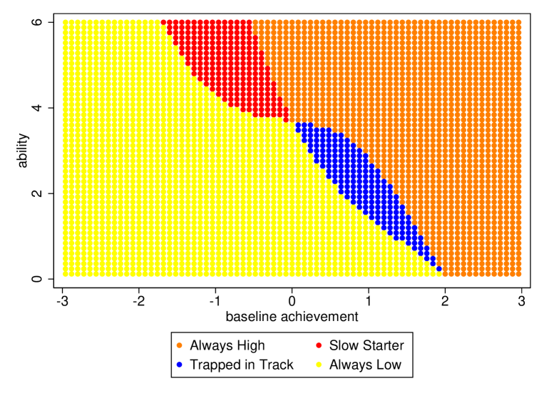
Figure 5: Student types, by baseline achievement and ability

It might sound curious at first, that there are students who would only reach the high track eventually, when they are initially assigned to the low track. Among practitioners however there seems to be some agreement that starting slow can be helpful in some cases. Within our model, the Slow Starter type has relatively high ability, but (relatively) low levels of baseline achievement. Hence, these students are underperforming in relation to their potential.

Table 2: Descriptive statistics

	(1)	(2)	(3)
	Total number	Single track	Fraction with test-based
Initial assignment	of students	level above	recom. at or above (2)
vmbo-bl	25,977	vmbo-kl	0.14
vmbo-kl	43,224	vmbo-gt	0.36
vmbo-gt	82,814	havo	0.21
havo	81,907	vwo	0.13
vmbo-bl / vmbo-kl	10,593	vmbo-kl	0.32
vmbo-kl / vmbo-gt	9,547	vmbo-gt	0.52
vmbo-gt / havo	25,437	havo	0.42
havo / vwo	29,616	vwo	0.32

• Notes. The table is based on the students in our final sample as discussed in Section 4. Column 1 presents the total number of students per initial track recommendation. Column 2 indicates the single track level that is directly above the initial track recommendation. Column 3 presents the fraction of students with a test-based track recommendation that corresponds to, or is higher than, the single track level of column 2.

Column 2 lists the single track levels that are directly above the initial track recommendations. Column 3 presents the fraction of students with a test-based track recommendation that corresponds to, or is higher than, the single track listed in column 2. In our analysis we estimate the treatment effects at the minimum test score (i.e. the test score cutoff) that is required for a test-based recommendation listed in column 2. For instance, for students in 2014/15 with a vmbo-gt or vmbo-gt/havo track recommendation the relevant cutoff is 537, which corresponds to a test-based havo recommendation (see Table LABEL:tab:toetsadvies in Appendix D). For students with a havo or havo/vwo recommendation the relevant cutoff is 545, which corresponds to a test-based vwo recommendation.

Column 3 shows that, in particular for students with a single track recommendation, the cutoff scores are relatively high scores in the conditional test score distribution. Depending on the initial recommendation, the test score cutoff is between the 64th and the 87th percentile of the conditional test score distribution. For students with a mixed recommendation, the cutoff level is approximately between the median and the 70th percentile.

5 The fuzzy RD specification and estimation

Our empirical counterpart for (4) is $\beta_{HH}$ in the following fuzzy RD model:

$$H_{4}\times H_{1}= \,\alpha_{HH}+\beta_{HH}H_{1}+f_{HH}(S)+\epsilon_{HH},$$ (8)

$$H_{1}= \,\delta_{H}+\pi_{H}Z+f_{H}(S)+\eta_{H},$$ (9)

where (8) is the second stage and (9) is the first stage. Our empirical counterparts for (5)-(7) are specified by replacing $H_{4}\times H_{1}$ and $H_{1}$ appropriately.

The polynomial $f(S)$ and bandwidth are important considerations for the fuzzy RD model in (8) and (9). Following Imbens and Lemieux (2008); Cattaneo et al. (2020), we specify a polynomial of degree one that is allowed to differ on each side of the cutoff. The Cito test score ranges from 501 to 550, and therefore has a discrete set of 50 points. We use a fixed bandwidth of three test score points on both sides of the cutoff. This bandwidth aligns well with results from the several data-driven bandwidth selection procedures using the Stata command rdrobust proposed by Calonico et al. (2017). Our fixed bandwidth across outcome variables ensures that our empirical counterparts for (4)-(7) exactly add up to two. We estimate the fuzzy RD model using 2SLS with robust standard errors, separately for each of the eight initial track recommendations shown in Table 4.2.

5.1 Testing the continuity assumption

Assumption 1a requires that students just to the left and right of the cutoff have similar potential outcomes. Though potential outcomes are unobserved, we can study whether students are similar on observable background characteristics via the following model:

$$X= \,\psi_{X}+\gamma_{X}Z+f_{X}(S)+\varepsilon_{X},$$ (10)

where $X$ is one of four student background characteristics: household income, migration background, age, and gender. If the estimates for $\gamma_{X}$ are statistically significant, assumption 1a may be violated. We estimate (10) using OLS separately for the eight track recommendations, using a polynomial of degree one and a bandwidth of three test score points. Table LABEL:tab:balance2 in Appendix B shows that our estimates for $\gamma_{X}$ are small and statistically insignificant at the 5% level for all four background characteristics across all eight track recommendations.

Figure B in Appendix B provides a visual representation of our results for (10) via RD plots. In particular, it plots the mean of household income at every test score point $S$ against the test score, which is normalized by subtracting the cutoff. The light grey area indicates the 95% confidence interval of each mean. The black line is a fourth order polynomial in $S$. The RD plot shows the full range of our data, using a bandwidth of 20 test score points. The figure confirms the results presented in Table LABEL:tab:balance2: students near the test score cutoffs seem comparable in terms of household income.

Second, we examine the continuity of the test score distribution (McCrary, 2008). If students have precise control over their test score, we might observe bunching just above the cutoffs and the continuity assumption may not be valid (Lee and Lemieux, 2010). Figure 4.2 in Appendix B plots the test score distribution for each of the three cohorts separately, and shows that the distribution is continuous throughout. These results are perhaps not surprising given the setting at hand. The Cito test only contains closed questions and is graded by a computer without interference from the primary school teacher. Hence, the scope for manipulation from students and teachers is limited.

5.2 Testing the first stages

Once students score above the relevant test score cutoff, they might receive a revised track recommendation and start secondary education in first year on a (relatively) high track. In this section we estimate the first stage in (9) with OLS, separately for each of the eight initial track recommendations. The estimates for $\pi_{H}$ measure to which extent a test score above the cutoff translates into high track enrollment in first year. In particular, they identify the proportion of compliers: the students that start in the high track because they score above the cutoff.

& vwo 16,199 0.102*** (0.012)

vmbo-gt havo 29,428 0.035*** (0.005)

vmbo-gt/havo havo 13,092 0.052*** (0.014)

vmbo-kl vmbo-gt 17,688 0.074*** (0.010)

vmbo-kl/vmbo-gt vmbo-gt 4,469 0.059* (0.032)

vmbo-bl vmbo-kl 6,357 0.005 (0.015)

vmbo-bl/vmbo-kl vmbo-kl 3,907 0.007 (0.031)

• Notes. ***, **, * refers to statistical significance at the 1, 5, and 10% level. Robust standard errors in parentheses. The first stage of the fuzzy RD in (9) uses a polynomial of order one, that is allowed to differ on each side of the cutoff, and a bandwidth of three test score points.

Table LABEL:tab:fs shows that, across the five initial track recommendations in the first five rows, the proportion of compliers is between 5 and 10%. Moreover, with $t$-statistics ranging between 5 and 10 for these five initial track recommendations, the effect of scoring above the cutoff on first-year track enrollment is strongly statistically significant. The first stage estimates for the three track assignments presented in row six unto eight of Table LABEL:tab:fs, however, are small and statistically insignificant at the 5% level. Since for these initial track recommendations we do not have a strong first stage, we do not present their second stage estimates in Section 6. Figure 5.2 visually confirms the strength of the first stage estimates for the initial track recommendations in first five rows of Table LABEL:tab:fs, using RD plots.

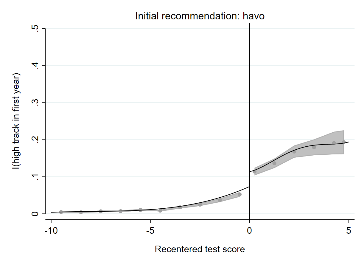
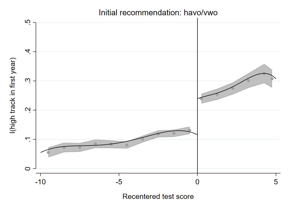
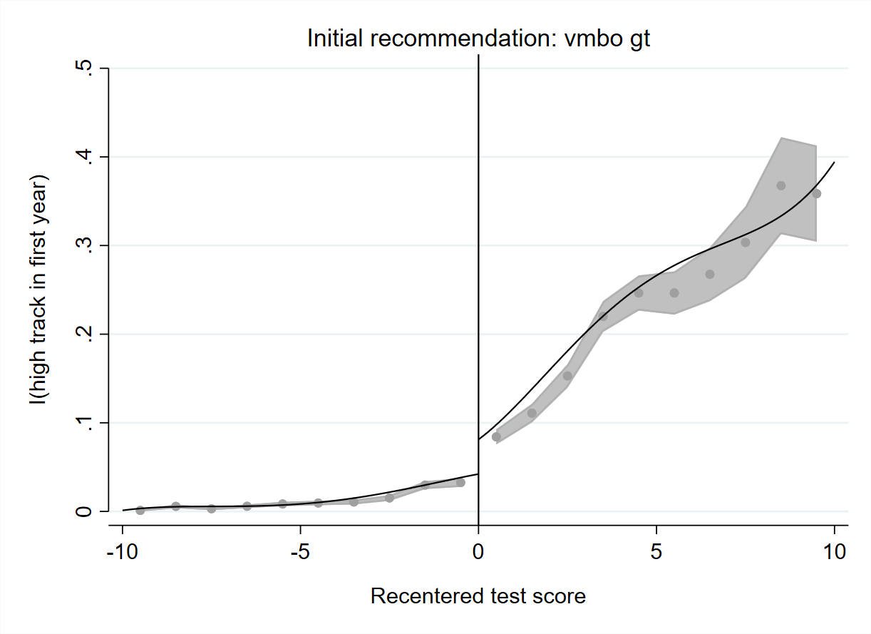
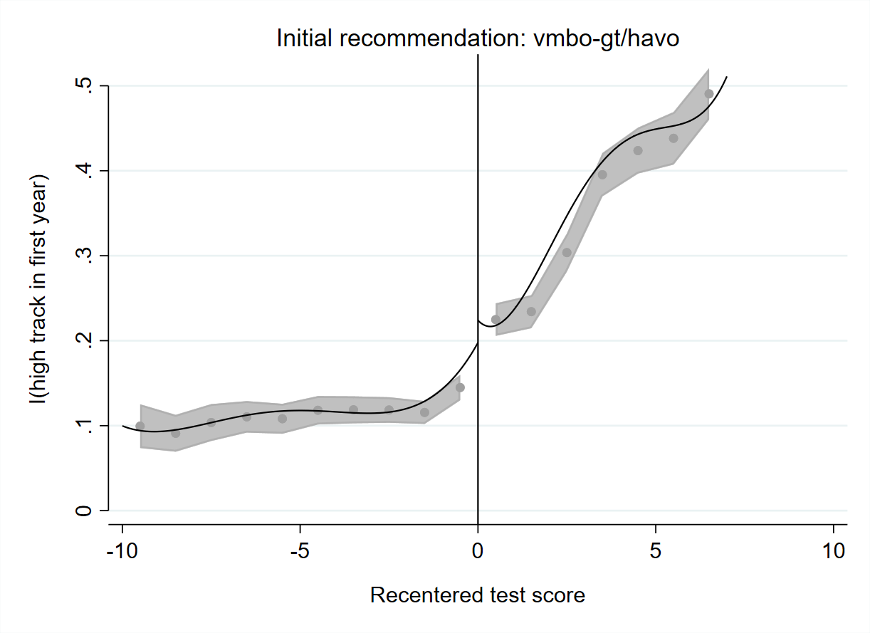
Figure 2: Visual representation of the first stages

Notes: Test scores are centered at the relevant cutoffs. Note that occasionally, students with the same initial recommendation are affected at more than one cutoff. This matters for example for students with a vmbo-gt recommendation, who are affected at the havo cutoff (at which the figure is centered), but also at the havo/vwo cutoff, which is at $+3$ test points on the recentered test score axis.

References

- Abadie (2002) Abadie, A. (2002). Bootstrap tests for distributional treatment effects in instrumental variable models. Journal of the American statistical Association 97(457), 284–292.
- Andresen and Huber (2021) Andresen, M. E. and M. Huber (2021). Instrument-based estimation with binarised treatments: issues and tests for the exclusion restriction. The Econometrics Journal 24(3), 536–558.
- Angrist and Imbens (1995) Angrist, J. D. and G. W. Imbens (1995). Two-stage least squares estimation of average causal effects in models with variable treatment intensity. Journal of the American statistical Association 90(430), 431–442.
- Calonico et al. (2017) Calonico, S., M. D. Cattaneo, M. H. Farrell, and R. Titiunik (2017). rdrobust: Software for regression-discontinuity designs. The Stata Journal 17(2), 372–404.
- Cattaneo et al. (2020) Cattaneo, M. D., N. Idrobo, and R. Titiunik (2020). A Practical Introduction to Regression Discontinuity Designs: Foundations. Elements in Quantitative and Computational Methods for the Social Sciences. Cambridge University Press.
- Duflo et al. (2011) Duflo, E., P. Dupas, and M. Kremer (2011). Peer effects, teacher incentives, and the impact of tracking: Evidence from a randomized evaluation in Kenya. American Economic Review 101(5).
- Dustmann et al. (2017) Dustmann, C., P. A. Puhani, and U. Schönberg (2017). The long-term effects of early track choice. The Economic Journal 127(603).
- Hoxby (2021) Hoxby, C. M. (2021). Advanced cognitive skill deserts in the united states: Their likely causes and implications. Brookings Papers on Economic Activity.
- Imbens and Lemieux (2008) Imbens, G. W. and T. Lemieux (2008). Regression discontinuity designs: A guide to practice. Journal of econometrics 142(2), 615–635.
- Janssen et al. (2021) Janssen, L. A., G. Huitsing, B. ter Beek, and A. C. Timmermans (2021). Gelijke kansen voor leerlingen met lager opgeleide ouders bij de overgang naar het voortgezet onderwijs? onderzoek naar schoolloopbanen en perspectieven van beslissers. Mens & Maatschappij.
- Kitagawa (2015) Kitagawa, T. (2015). A test for instrument validity. Econometrica 83(5), 2043–2063.
- Kwak and Lee (2023) Kwak, D. W. and J. Y. Lee (2023). Attending a school with heterogeneous peers: The effects of school detracking and its attenuation. Economics of Education Review 94.
- Lee and Lemieux (2010) Lee, D. S. and T. Lemieux (2010). Regression discontinuity designs in economics. Journal of economic literature 48(2), 281–355.
- McCrary (2008) McCrary, J. (2008). Manipulation of the running variable in the regression discontinuity design: A density test. Journal of econometrics 142(2), 698–714.
- Oosterbeek et al. (2021) Oosterbeek, H., S. ter Meulen, and B. van der Klaauw (2021). Long-term effects of school-starting-age rules. Economics of Education Review 84.
- Pritchett and Beatty (2015) Pritchett, L. and A. Beatty (2015). Slow down, you’re going too fast: Matching curricula to student skill levels. International Journal of Educational Development 40.
- WPO (2014) WPO (2014). Artikel 42, lid 2, Wet op het primair onderwijs. Datum inwerkingtreding: 01/08/2014. wetten.overheid.nl.
- WVO (2014) WVO (2014). Artikel 3, lid 2, Inrichtingsbesluit Wet op het voortgezet onderwijs. Datum inwerkingtreding: 01/08/2014. wetten.overheid.nl.