An Attention Free Conditional Autoencoder For Anomaly Detection in Cryptocurrencies

Abstract

It is difficult to identify anomalies in time series, especially when there is a lot of noise. Denoising techniques can remove the noise but this technique can cause a significant loss of information. To detect anomalies in the time series we have proposed an attention free conditional autoencoder (AF-CA). We started from the autoencoder conditional model on which we added an Attention Free LSTM layer Inzirillo and De Villelongue (2022) in order to make the anomaly detection capacity more reliable and to increase the power of anomaly detection. We compared the results of our Attention Free Conditional Autoencoder with those of an LSTM Autoencoder and clearly improved the explanatory power of the model and therefore the detection of anomaly in noisy time series.

1 Introduction

To identify anomalies in prices on a basket of cryptocurrencies returns, autoencoders can prove themself useful. An autoencoder is a type of neural network in which outputs try to approximate inputs variables. It is divided in two steps, the first one is the encoding part where the input variable is passed inside a small number of neurons in the hidden layers, creating a compressed representation of the input and the second the decoding step which unpack the input representation and maps it to the output layer. An autoencoder with no other variable than inputs can thus be qualified as a dimension reduction and unsupervised learning device. Self attention mechanisms Zhai et al. (2021) embedded within the Transformer allows to increase the efficiency of learning task in machine translation, language understanding and other paradigms. We introduce an Attention Free LSTM Autoencoder, able to focus on input sequence that will have an impact on prediction. In a latter paper Gu et al. (2021) introduced non linear functions to identify latent factors of random variables, however they use LSTM layers, which turns out to be less effective than models based on attention mechanisms Zeyer et al. (2019). In this paper we look for an architecture to detect anomalies which led us to identify the importance of factors of our time series. Zhai et al. (2021) presented a Attention Free Transformer (AFT) more efficient than Transformer Vaswani et al. (2017) during the learning task, so we started from this point and added and attention free mechanism in the encoder-decoder strucutre to only capture the variables that have a positive impact and minimized the recontruction error. The Attention Free Autoencoder structure we present allows us to better identify anomalies in time series.

2 Factor Models

Gu et al. (2021) proposed a new model to estimates latent factors for stochastic time series. They started from the work of Kozak (2019) however they introduced non-linear functions to estimate nonlinear conditional exposures and latent factors associated.

2.1 Linear Factor Models

When the autoencoder has one hidden layer and a linear activation function, it is equivalent to the PCA estimator for linear factor models The static linear factor model is written:

$$y_{t}=\beta X_{t}+u_{t},$$ (1)

$\left(Y_{t}\right)_{0{\leq k}{\leq T}}$ is a vector of random variables, $y_{t}$ is a random variable, $y_{t}\in\mathbb{R}$ and $X_{t}$ is a $K$ × $1$ vector of factors, $u_{t}$ is a $N$ × $1$ vector of idiosyncratic errors (independant of $X_{t}$), and $\beta$ is the $N$ × $K$ matrix of factor loadings. The matrix form of the factor model is given by:

$$Y=\beta X+U.$$ (2)

2.2 Non Linear Factor Models

A gain in precision can be obtained by incorporating asset-specific covariates in the specification of factor loadingsGu et al. (2021). These covariate also indirectly improve estimates of the latent factors themselves. Their model formulation amounts to a combination of two linear models:

• A linear specification for the latent factors, that models the factor loadings as a nonlinear function of covariates, given by:

  $$y_{i,t}=\beta_{i,t-1}X_{t}+u_{i,t}$$ (3)

• A linear specification for conditional betas, that models factors as portfolios of individual stock returns, obtained from:

  $$\beta(z_{i,t-1})=z_{i,t-1}\Gamma$$ (4)

3 Autoencoders

Autoencoders Hinton and Salakhutdinov (2006) are a type of artificial neural network trained to reconstruct their input, which forces them to learn a compressed representation of the data. Autoencoders is an unsupervised learning task that can be used for dimensionality reduction as well as feature extraction. There is a close connection between autoencoders and PCA Baldi and Hornik (1989) and, by extension, between autoencoders and latent factor asset pricing models Gu et al. (2021).

3.1 Simple Linear Autoencoder

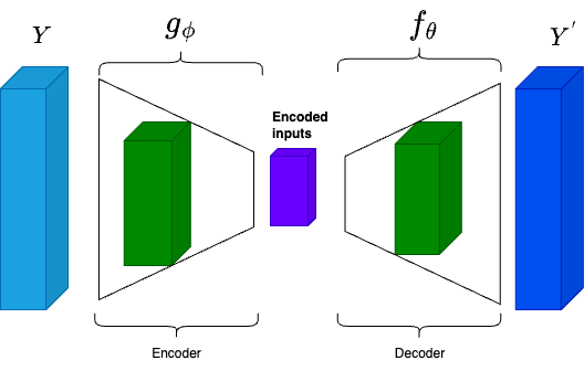
Figure 1: Linear Autoencoder

Let us define $\phi$ and $\theta$ the encoder and decoder set of parameters, respectively. Where $\phi:=\{\phi^{(0)},\phi^{(1)}\}$ and $\theta:=\{\theta^{(0)},\theta^{(1)}\}$ We can write the one-layer, linear autoencoder with K neurons as:

$$\begin{split}y_{t}&=f_{\theta}(g_{\phi}(y_{t}))+u_{t},\\ &=\theta^{(0)}+\theta^{(1)}(\phi^{(0)}+\phi^{(1)}y_{t})+u_{t},\end{split}$$ (5)

where $\phi^{(1)}$ $\theta^{(1)}$, $\theta^{(0)}$ and $\phi^{(0)}$ are $K$ × $N$, $N$ ×$K$, $N$ × $1$, and $K$ × $1$ matrices of parameters, respectively. The objective of the model is to minimize the reconstruction error $u_{t}$ for each time step. $u_{t}$ is defined as :

$$u_{t}=y_{t}-f_{\theta}(g_{\phi}(y_{t})).$$ (6)

The parameters of the encoder and the decoder $\phi$ and $\theta$ can be estimated by solving the following optimization problem:

$$\min_{\phi,\theta}\sum_{t=1}^{T}\left\lVert y_{t}-(\theta^{(0)}+\theta^{(1)}(\phi^{(0)}+\phi^{(1)}y_{t}))\right\rVert^{2}.$$ (7)

3.2 Conditional Linear Autoencoders

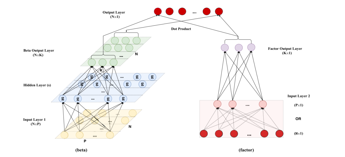
Figure 2: Conditional Autoencoders Structure Gu et al. (2021)

Figure 2 illustrates the structure of the conditional autoencoder introduced by Gu et al. (2021). The left side of the network models factor loadings as a nonlinear function of covariates. This covariates can be characteristics of the time series, such technical indicators. The right side network models factors as portfolios of individual crypto-currency returns.

$$y_{i,t}=\beta_{i,t-1}f_{t}+u_{i,t},$$ (8)

The recursive formulation for the nonlinear beta function is:

$$\begin{split}z_{i,t-1}^{(0)}&=z_{i,t-1},\\ z_{i,t-1}^{(l)}&=g(b^{(l-1)}+W^{(l-1)}z_{i,t-1}^{(l-1)}),\ l=1,...,L_{\beta}\\ \beta_{i,t-1}&=b^{(L_{\beta})}+W^{(L_{\beta})}z_{i,t-1}^{(L_{\beta})}.\\ \end{split}$$ (9)

The recursive mathematical formulation of the factors is:

$$\begin{split}y_{t}^{(0)}&=y_{t}\\ y_{t}^{(l)}&=\tilde{g}(\tilde{b}^{(l-1)}+\tilde{W}^{(l-1)}y_{t}^{(l-1)}),\ l=1,...,L_{f}\\ X_{t}&=\tilde{b}^{(L_{f})}+\tilde{W}^{(L_{f})}y_{t}^{(L_{f})}\end{split}$$ (10)

3.3 Conditional Attention Free Autoencoders

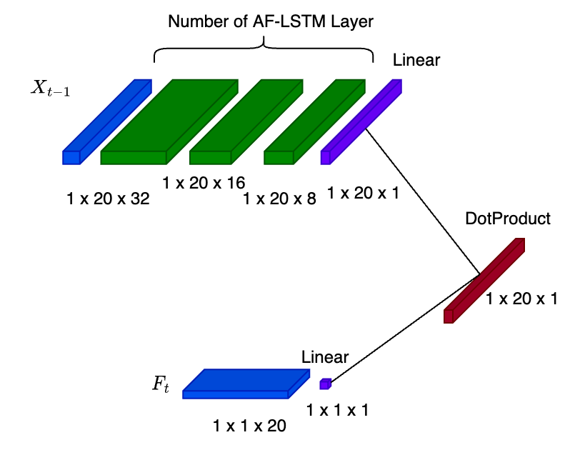
Figure 3: Conditional Attention Free Autoencoder

3.3.1 LSTM

The LSTM framework Hochreiter and Schmidhuber (1997) are RNNs with gated mechanisms designed to avoid vanishing gradient. The blocks of LSTM contain 3 non-linear gates; input gate, forget gate and output gate. This architecture embedded a memory for sequences that increase the power of prediction for time series forecasting.

• Input gate ($i_{t}$): decides which values from the input are used to update the memory,

• Forget gate ($f_{t}$): handles what information to throw away from the block,

• Output gate ($o_{t}$): handles what will be in output based on input and memory gate.

During the training step, each iteration provides an update of the model weights proportional to the partial derivative and in some cases the gradient may be vanishingly small and weights may not be updated. The LSTM networks is defined in Figure 4 as:

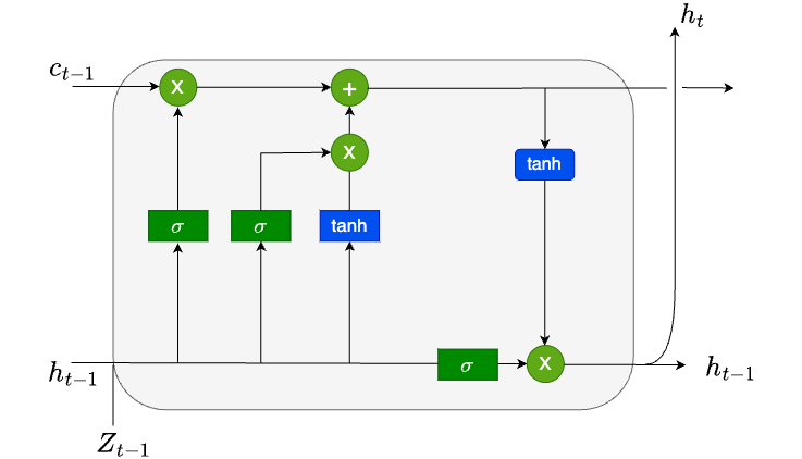
Figure 4: LSTM Cell

$$\begin{split}f_{t}&=\sigma(W_{f}[h_{t-1},z_{t-1}]+b_{f})\\ i_{t}&=\sigma(W_{i}[h_{t-1},z_{t-1}]+b_{i})\\ {\tilde{c}}_{t}&={\tanh(W_{c}[h_{t-1},z_{t-1}]+b_{c})}\\ c_{t}&=f_{t}\odot c_{t-1}+i_{t}\odot{\tilde{c}}_{t}\\ o_{t}&=\sigma(W_{o}[h_{t-1},z_{t-1}]+b_{o})\\ h_{t}&=o_{t}\odot{\tanh(c_{t})}\end{split}$$ (11)

where $\Theta:=\{W_{f},W_{i},W_{c},W_{o}\}$ is the set of model parameters and $z_{t-1}$ is the input vector at time t containing all the past information. The number of parameters of each layer in the model should be carefully selected to handle overfitting or underfitting situations.

3.3.2 Attention Free Mechanism

The transformer architecture has made it possible to develop new models capable of being trained on large dataset while being much better than recurrent neural networks such as LSTM. The Attention Free Transformer Zhai et al. (2021) introduces the attention free block, an alternative to attention block Vaswani et al. (2017), which eliminates the need for dot product self attention. The transformer is an efficient tool to capture the long term dependency. Just like the transformer, the AF Block includes interactions between queries, keys and values. The difference is that the AF block firstly combines key and value together with a set of learned position biases described in Zhai et al. (2021). Then the query is combined with the context vector. Let Q, K, V denote the query, key and value, respectively.

$$\begin{split}Y_{t}&=\sigma_{q}(Q_{t})\odot\frac{\sum_{t^{{}^{\prime}}=1}^{T}exp(K_{t^{{}^{\prime}}}+w_{t,t^{{}^{\prime}}})\odot V_{t^{{}^{\prime}}}}{\sum_{t^{{}^{\prime}}=1}^{T}exp(K_{t^{{}^{\prime}}}+w_{t,t^{{}^{\prime}}}))}\\ &=\sigma_{q}(Q_{t})\odot\sum_{t^{{}^{\prime}}=1}^{T}(\text{Sofmax}(K)\odot V)_{t{{}^{\prime}}}\end{split}$$ (12)

where $Q=ZW_{q}$, $K=ZW_{k}$ and $V=ZW_{v}$. The activation function $\sigma_{q}$ is the sigmoid function and $w_{t}\in\mathbb{R}^{T\times T}$ is a learned matrix of pair-wise position biases.

3.4 Attention Free LSTM

The attention mechanism Vaswani et al. (2017) allows the encoder-decoder models based to be trained only on specific parts of a data sequence that will contribute positively to the prediction of an output, in our case part of the past observations will be kept in order to predict the output of our Conditional Autoencoder. Gu et al. (2021) uses only linear layers to encode and decode the input sequence without necessarily considering temporality and memory. The Attention-Free LSTM Layer Inzirillo and De Villelongue (2022) , brings in addition to the memory effect the possibility to take into account only the necessary input and to filter this input in order to predict the output. The AF-LSTM Layer embeds an attention mechanism as well as an activation function that will allow to eliminate a part of the input sequence that is not useful for the reconstruction of this sequence.

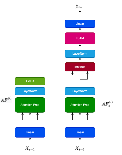
Figure 5: Attention-Free LSTM LayerInzirillo and De Villelongue (2022)

Our $input\_tensor$ for each layer denoted $X$ will be filtered on the left side Figure 5 using an attention mechanism and an activation function (ReLU) to only propagte the revelant information for prediction throught the other hidden layers denoted $l$. Which can be mathematically written such:

$$\tilde{X}_{i,t-1}^{(l)}=AF^{(l)}_{1}(W_{i,1}^{(l)};X_{i,t-1}),\quad i:=\{1,...,N\}.$$ (13)

where $X_{t}\in\mathbb{R}^{N}$ and $AF^{(l)}_{i,1}$ is the Attention Free of the $l-th$ layer for the $i-th$ time series is defined as:

$$\begin{split}x_{i,t-1}^{(l)}&=\text{Concat}(W_{x}^{(l)}X_{i,t-1}+b_{x}^{(l)}),\\ Q_{i,t-1}^{(l)}&=W_{q}^{(l)}x_{i,t-1}^{(l)},\\ K_{i,t-1}^{(l)}&=W_{k}^{(l)}x_{i,t-1}^{(l)},\\ V_{i,t-1}^{(l)}&=W_{v}^{(l)}x_{i,t-1}^{(l)},\\ \eta_{i,t-1}^{(l)}&=\sum_{t=1}^{T}\text{Softmax}(K_{i,t-1}^{(l)})\odot V_{i,t-1}^{(l)},\\ \tilde{X}_{i,t-1}^{(l)}&=\sigma(Q_{i,t-1}^{(l)})\odot\eta_{i,t-1}^{(l)}.\\ \end{split}$$ (14)

we apply the Layer Normalization (LN) function Ba et al. (2016) was developed to compensate the summed input of reccurent neurons.

$$LN(x;\psi;\phi)=\psi\frac{(x-\mu_{x})}{\sigma_{x}}+\phi,$$

and filter our $\tilde{X}_{t-1}$ using the ReLU activation function, $ReLU(x)=max(0,x)$.

Hence we have:

$$\tilde{x}_{t-1}=ReLU(LayerNorm(\tilde{X}_{t-1})),$$ (15)

$$\begin{split}\bar{X}_{i,t-1}&=AF_{i,2}^{(l)}(W_{i,2}^{(l)};X_{t-1}),\\ \bar{x}_{i,t-1}&=LN(\bar{X}_{t-1};\psi^{(l)};\phi^{(l)}).\end{split}$$ (16)

The output from the two channels will be multiplied to apply the filter on our input sequence.

$$\begin{split}\eta_{i,t-1}^{(l)}&=(\tilde{x}_{i,t-1}\odot\bar{x}_{i,t-1}),\\ \zeta_{i,t-1}^{(l)}&=LN(\eta^{(l)};\psi^{(l)};\phi^{(l)}).\end{split}$$ (17)

$\zeta_{t-1}^{(l)}$ will be the input of a parametrized function $g_{w}^{(l)}$ such:

$$h_{i,t-1}^{(l)}=g_{w}^{(l)}(\zeta_{i,t-1}^{(l)}),$$ (18)

in Figure 5 $g_{w}^{(l)}(.)$ is a LSTM Figure 4. Using the output of $g_{w}^{(l)}(.)$ we can estimate the output of the $l-th$ layer $\beta_{i,t-1}^{(l)}$ given by:

$$\beta_{i,t-1}^{(l_{\beta})}=W_{y}^{(l_{\beta})}h_{i,t-1}^{(l_{\beta})}+b_{y}^{(l_{\beta})},\quad l:=\{1,...,l_{\beta}\}.$$ (19)

4 Learning task

4.1 Datasets

We take one year of hourly data to perform our analysis on 20 cryptocurrencies. We retrieve the OHLC and volume from CryptoCompare and calculate five indicators with the Pandas TA : the SMA on 24 hours, the DEMA on 12 hours, the CCI on 24 hours, the AD and the ATR on 24 hours. We then add the time varying hurst exponent by computing log returns, which will be used in the factors part of our models. Finally, we compute the returns on which we will perform training to get predictions. In our models, X1 corresponds to the 5 factors values evolution, X2 to the hurst exponent evolution with 1 lag and Y to the returns evolution with 1 lag. We rank-normalize asset characteristics into the interval (-1,1) for X1 and Y to create tensors scalers.Afterwards, the train set for X1 and Y are fitted and transformed, and the test set for X1 and Y only transformed. The fit method is calculating the mean and variance of each of the features present in the data. The transform method is transforming all the features using the respective mean and variance. The parameters learned by the model using the training data will help to transform the test data.

We finally divide our sample into three time periods to maintain temporal ordering:

• The first sample is used for training the model, subject to a specific set of hyperparameter values. It corresponds to 70 percent of 1 year of hourly data.

• The second sample is used for validation to tune the hyperparameters. It corresponds to 15 percent of 1 year of hourly data, beginning after the training set.

• The third and last sample is the testing sample used to evaluate a model. It corresponds to the last 15 percent of 1 year of hourly data.

4.2 Autoencoders Types

For our study we have compared three types of models. Three autoencoders have been implemented:

• Simple autoencoders using linear layers as encoders and decoders. It takes as parameters the input and hidden size or the hidden size and output size.

• LSTM autoencoders using LSTM layers as encoders and decoders. It takes as parameters the input and hidden size or the hidden size and output size.

• AF LSTM autoencoders using AF LSTM layers as encoders and decoders. It takes as parameters the input size, hidden size, the maximum length of the sequence and the output size.

4.3 Autoencoders Dimensions

The inputs and outputs of the networks are the following:

• Input of the Beta Network : 5 which corresponds to the 5 factors in X1.

• Input of the Factor Network : 20 which corresponds to the 20 cryptocurrencies selected.

• Output of the Beta Network : 1 which is selected as parameter of the models.

• Output of the Factor Network : 1 which is selected as parameter of the models.

Autoencoders with various degrees of complexity are created:

• The simplest, which we denote CA0, uses a single linear layer in both the beta and factor networks.

• CA1 which adds a hidden layer with 32 neurons in the beta network.

• CA2 which adds a second hidden layer with 16 neurons in the beta network.

• CA3 which adds a third hidden layer with 8 neurons in the beta network.

4.4 Regularization

To prevent overfitting, several regularization techniques are implemented:

• Append a penalty to the objective function. In our case the LASSO or ‘l1’ penalization is used. The l1 penalty is set to 0.01 for the simple autoencoders, 0.0016 for the LSTM autoencoders and 0.0000012 for the AF LSTM autoencoders.

• Implement an early stopping tha terminates the optimization when the validation sample errors begin to increase. The tolerance for the early stopping is set to 10.

• Adopt an ensemble approach to train the neural networks. 10 multiple random seeds initialize the neural network estimation and construct model predictions by averaging estimates from all networks. This enhances the stability as different seeds can settle at different optima.

4.5 Optimization

To reduce the computational intensity of neural networks optimization in computing the loss function, the following algorithms can be added inside the autoencoders models:

• A stochastic gradient descent (SGD) with an Adam extension to train a neural network that sacrifices accuracy to accelerate the optimization routine. A critical tuning parameter in SGD is the learning rate, which is set to 0.001 for the three types of autoencoders tested.The number of epochs in our case is set to 200.

• The batch normalization that performs one activation over one batch on 20 batches.

• The layer normalization that normalizes the activations of the previous layer for each given example in a batch independently, rather than across a batch like batch Normalization. It is very effective at stabilizing the hidden state dynamics in recurrent networks. It takes the hidden size of the model as input.

4.6 Anomaly identification

We assume that our model is capable of estimating the factors and that its explanatory power is such that the little information it fails to explain through the determined factors indicates the presence of an anomaly or several anomalies. To identify theses anomalies in log returns, we collect the residuals obtained for the train and test sets. The extreme values at a 1 and 5 percent levels are then saved and compared to the log returns observed at the same time. We then consider the log return as abnormal and subject to a market anomaly.

5 Results

In this section we will analyze the results for Bitcoin and Ethereum only, which are the two largest cryptocurrencies in terms of market capitalization. The results for the other assets are available in the appendix.

5.1 Bitcoin Anomalies Detection

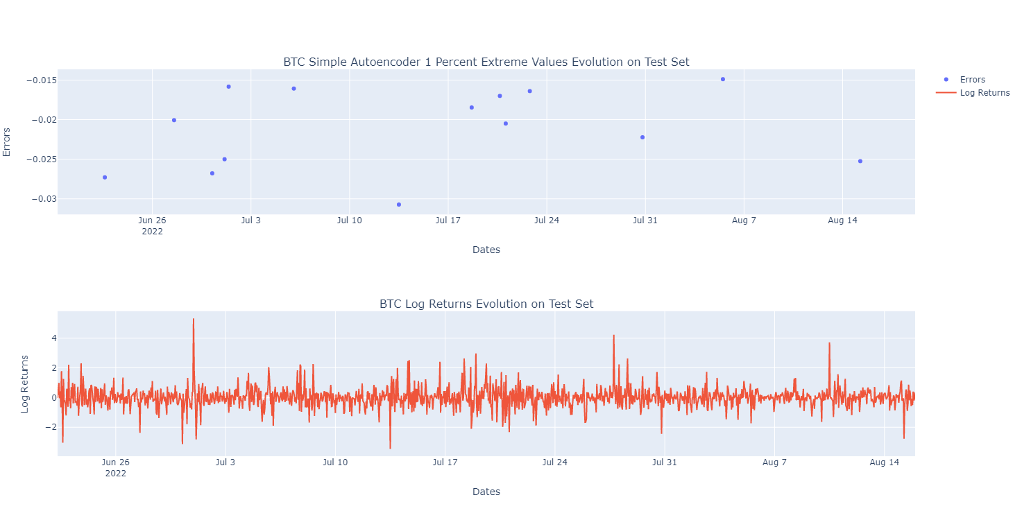
Figure 6: BTC Simple Autoencoder 1 Percent Extreme Values Evolution on Test Set

Figure 7: BTC LSTM Autoencoder 1 Percent Extreme Values Evolution on Test Set

Figure 8: BTC AF LSTM Autoencoder 1 Percent Extreme Values Evolution on Test Set

The Simple Autoencoder model in Fig.6 is able to catch nearly all the plummet phases in log returns. Its squared errors are the smallest of the three models.This model thus focuses more on predictions’ quality at the expense of anomalies detection precision. The LSTM autoencoder model in Fig.7 is catching an additional anomaly on the 30th of June at 1:00pm, which was ommited by the simple autoencoder model. It is not considering the 5th of August at 12:00pm as an anomaly, which could be seen as an incorrect classification by the simple autoencoder model. Its squared errors are the highest of the three models. This model thus focuses more on anomalies detection precision at the expense of predictions’ quality and finally AF LSTM autoencoder model in Fig.8 benefits from both the power of the Simple Autoencoder and the LSTM Autoencoder in returns prediction and anomaly detection.

5.2 Ethereum Anomalies Detection

Figure 9: ETH Simple Autoencoder 1 Percent Extreme Values Evolution on Test Set

Figure 10: ETH LSTM Autoencoder 1 Percent Extreme Values Evolution on Test Set

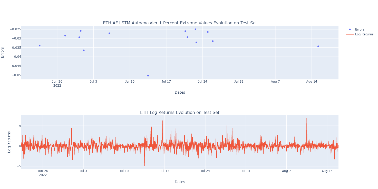
Figure 11: ETH AF LSTM Autoencoder 1 Percent Extreme Values Evolution on Test Set

The Simple Autoencoder model in Fig.9 has a good predictive power. Like the BTC, its squared errors are the smallest of the three models. The LSTM autoencoder model in Fig.10 is enlighting extra anomalies on the 30th of June at 1:00pm as well as on the 16th of July at 5:00pm. However it does not classify the 22nd of July at 3:00pm as well as the 24th of July at 12:00pm as anomalies. Like the BTC, its squared errors are the highest of the three models and finally AF LSTM autoencoder model in Fig.11 is not classifying the 16th of July at 5:00pm as an anomaly like the LSTM model but includes the 22nd of July at 3:00pm.

6 Conclusion

Although unsupervised techniques are powerful in detecting outliers, they are subject to overfitting and results that might be unstable.Training multiple models to aggregate the scores can be useful to detect how a change in the network structure can change the algorithms precision in predictions or their capacity to detect anomalies. Outlier detection is a by-product of dimension reduction, explaining the use of autoencoders in our models. The autoencoder techniques can perform non-linear transformations with their non-linear activation function and multiple layers. Instead of providing labels that classify the input features, we compare the prediction of the Autoencoder with the initial input features. It turns out that the AF-CA has a higher explanatory power than the classical autoencoder and thus allows us to better identify anomalies for very noisy time series. In a future work it would be interesting to look at the detection of anomalies in different market regimes, bullish as well as bearish knowing that cryptocurrencies have for main characteristic to be highly volatile assets.

7 Appendix

Figure 12: XRP Simple Autoencoder 1 Percent Extreme Values Evolution on Test Set

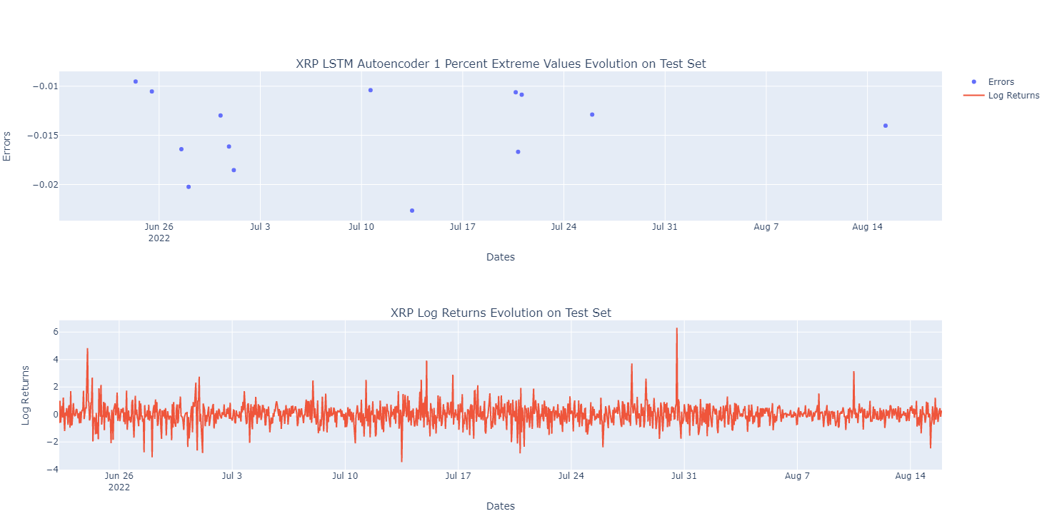
Figure 13: XRP LSTM Autoencoder 1 Percent Extreme Values Evolution on Test Set

Figure 14: XRP AF LSTM Autoencoder 1 Percent Extreme Values Evolution on Test Set

Figure 15: SOL Simple Autoencoder 1 Percent Extreme Values Evolution on Test Set

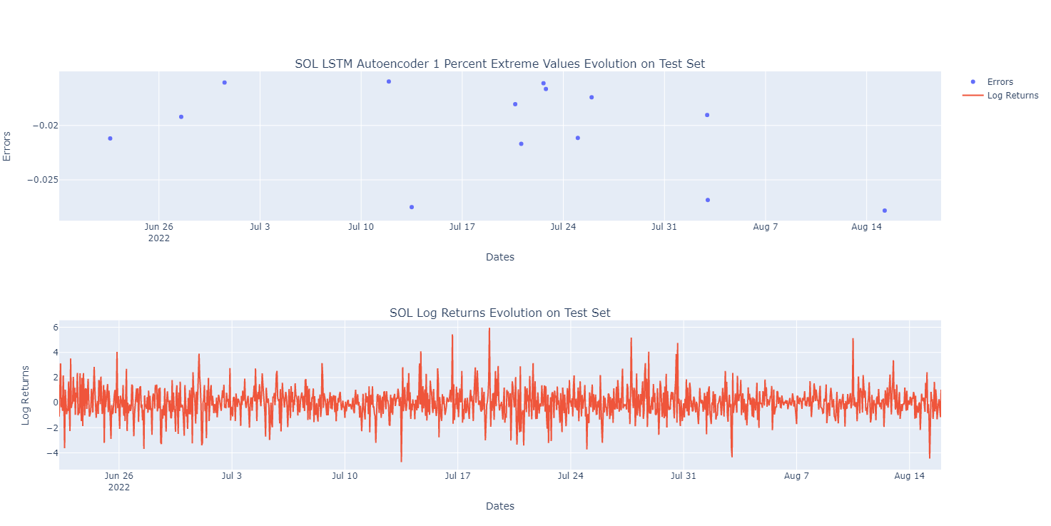
Figure 16: SOL LSTM Autoencoder 1 Percent Extreme Values Evolution on Test Set

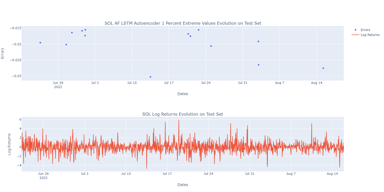
Figure 17: SOL AF LSTM Autoencoder 1 Percent Extreme Values Evolution on Test Set

Figure 18: SHIB Simple Autoencoder 1 Percent Extreme Values Evolution on Test Set

Figure 19: SHIB LSTM Autoencoder 1 Percent Extreme Values Evolution on Test Set

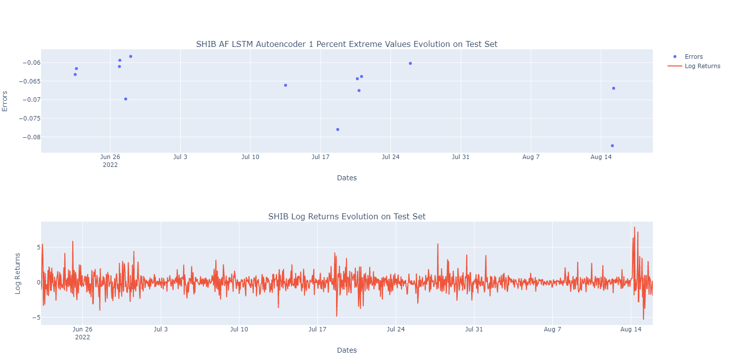
Figure 20: SHIB AF LSTM Autoencoder 1 Percent Extreme Values Evolution on Test Set

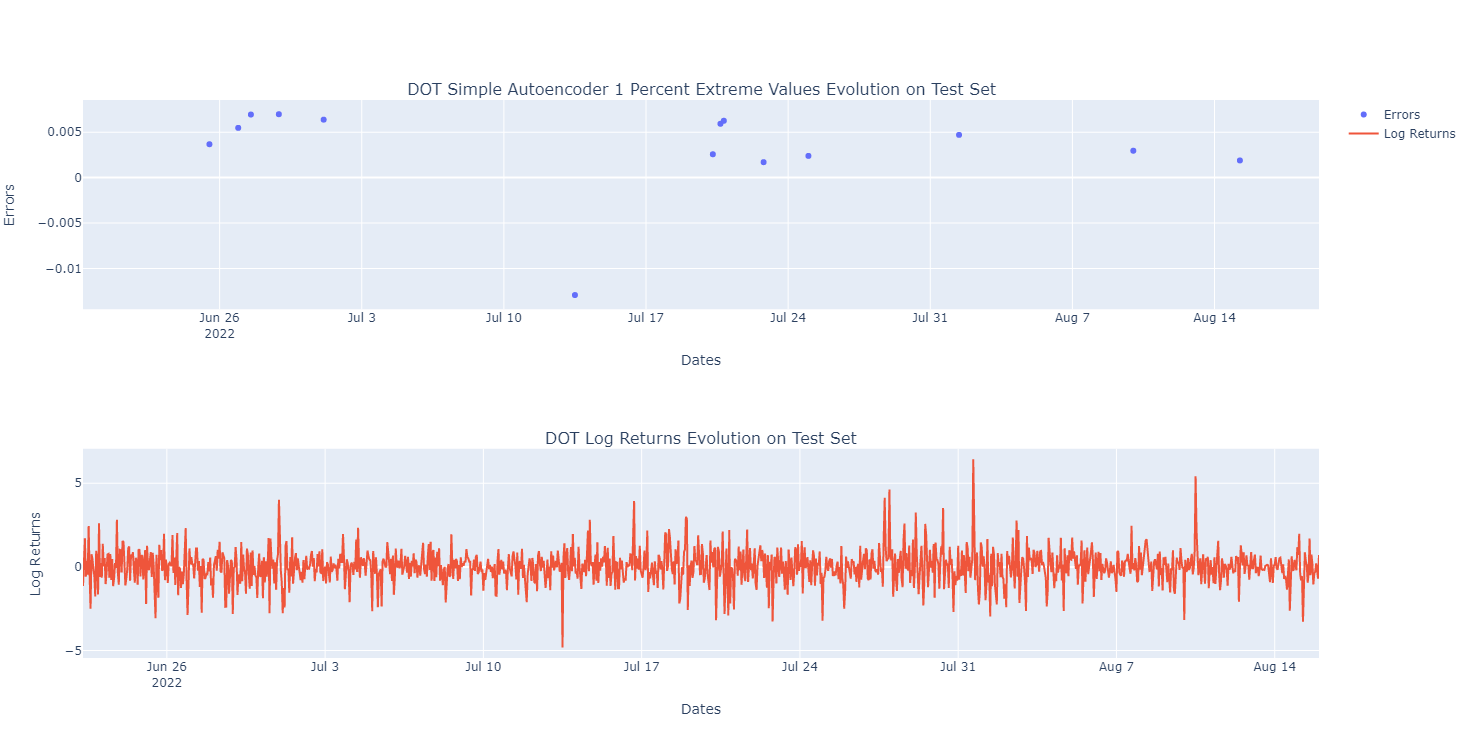
Figure 21: DOT Simple Autoencoder 1 Percent Extreme Values Evolution on Test Set

Figure 22: DOT LSTM Autoencoder 1 Percent Extreme Values Evolution on Test Set

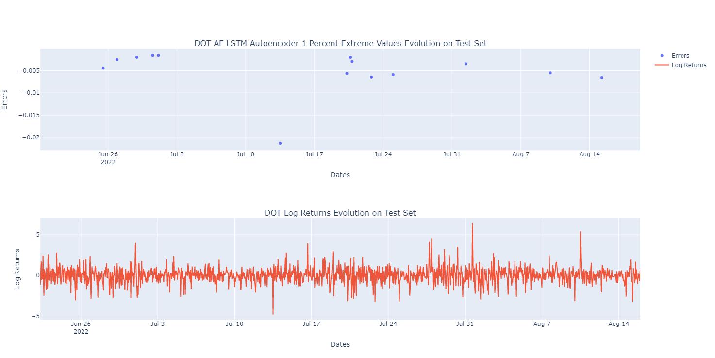
Figure 23: DOT AF LSTM Autoencoder 1 Percent Extreme Values Evolution on Test Set

Figure 24: BNB Simple Autoencoder 1 Percent Extreme Values Evolution on Test Set

Figure 25: BNB LSTM Autoencoder 1 Percent Extreme Values Evolution on Test Set

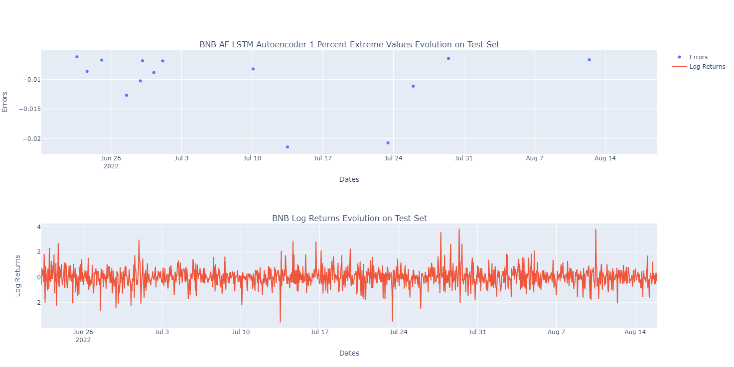
Figure 26: BNB AF LSTM Autoencoder 1 Percent Extreme Values Evolution on Test Set

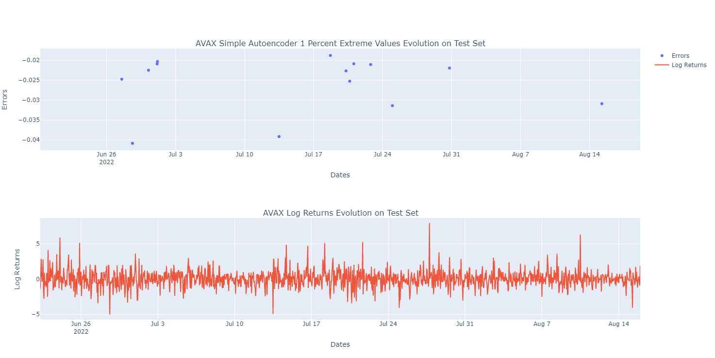
Figure 27: AVAX Simple Autoencoder 1 Percent Extreme Values Evolution on Test Set

Figure 28: AVAX LSTM Autoencoder 1 Percent Extreme Values Evolution on Test Set

Figure 29: AVAX AF LSTM Autoencoder 1 Percent Extreme Values Evolution on Test Set

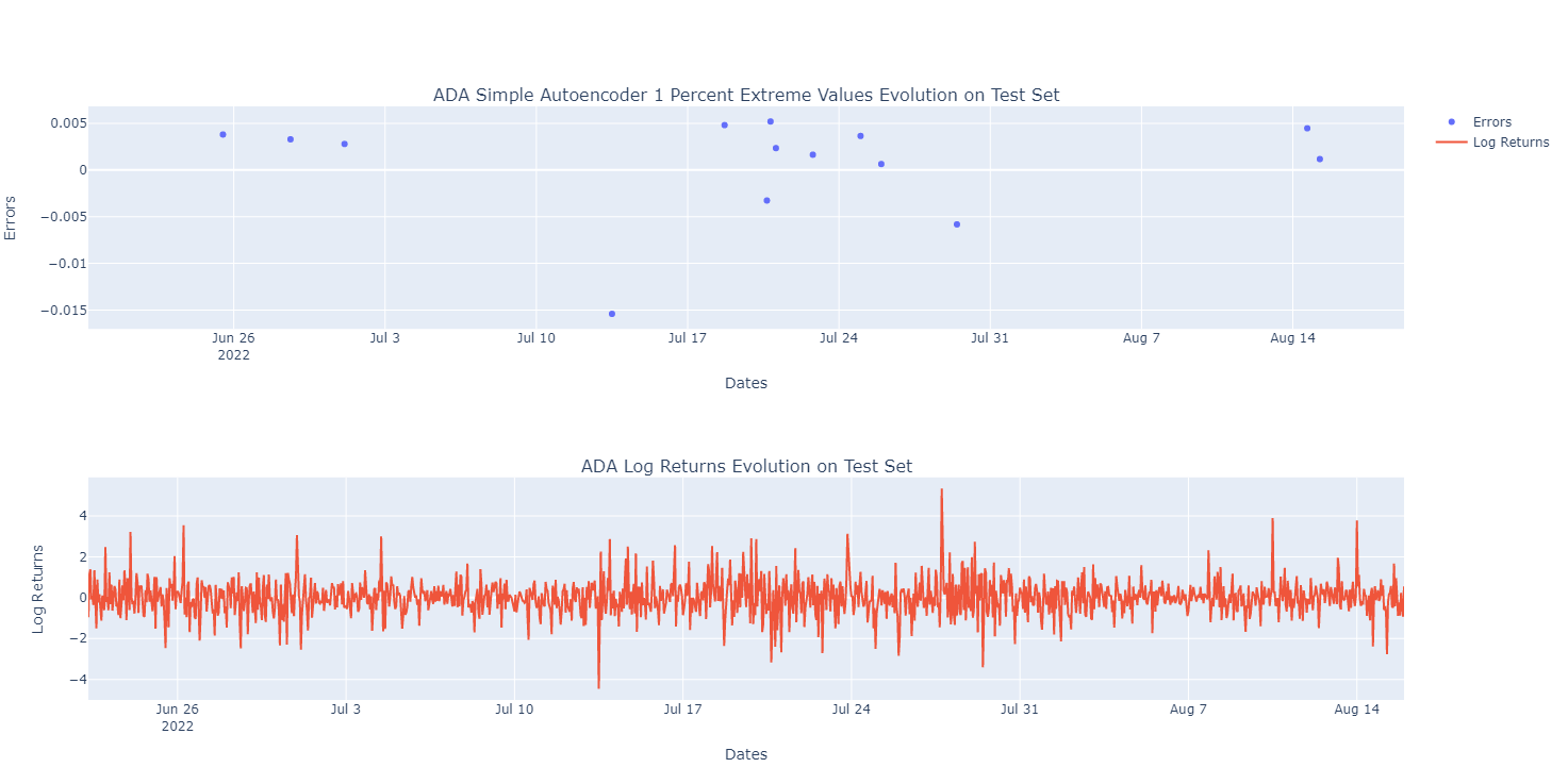
Figure 30: ADA Simple Autoencoder 1 Percent Extreme Values Evolution on Test Set

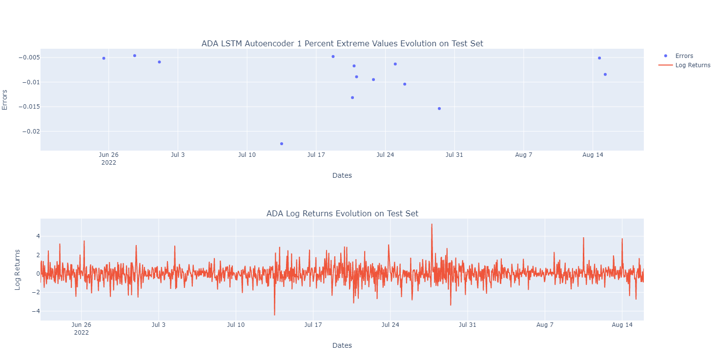
Figure 31: ADA LSTM Autoencoder 1 Percent Extreme Values Evolution on Test Set

Figure 32: ADA AF LSTM Autoencoder 1 Percent Extreme Values Evolution on Test Set

References

- Ba et al. [2016] Jimmy Lei Ba, Jamie Ryan Kiros, and Geoffrey E. Hinton. Layer normalization, 2016.
- Baldi and Hornik [1989] Pierre Baldi and Kurt Hornik. Neural networks and principal component analysis: Learning from examples without local minima. Neural networks, 2(1):53–58, 1989.
- Gu et al. [2021] Shihao Gu, Bryan Kelly, and Dacheng Xiu. Autoencoder asset pricing models. Journal of Econometrics, 222(1):429–450, 2021.
- Hinton and Salakhutdinov [2006] Geoffrey E Hinton and Ruslan R Salakhutdinov. Reducing the dimensionality of data with neural networks. science, 313(5786):504–507, 2006.
- Hochreiter and Schmidhuber [1997] Sepp Hochreiter and Jürgen Schmidhuber. Long short-term memory. Neural computation, 9:1735–80, 12 1997.
- Inzirillo and De Villelongue [2022] Hugo Inzirillo and Ludovic De Villelongue. An attention free long short-term memory for time series forecasting. arXiv preprint arXiv:2209.09548, 2022.
- Kozak [2019] Serhiy Kozak. Kernel trick for the cross section. SSRN Electronic Journal, 01 2019. doi: 10.2139/ssrn.3307895.
- Vaswani et al. [2017] Ashish Vaswani, Noam Shazeer, Niki Parmar, Jakob Uszkoreit, Llion Jones, Aidan N. Gomez, Lukasz Kaiser, and Illia Polosukhin. Attention is all you need. CoRR, abs/1706.03762, 2017.
- Zeyer et al. [2019] Albert Zeyer, Parnia Bahar, Kazuki Irie, Ralf Schluter, and Hermann Ney. A comparison of transformer and lstm encoder decoder models for asr. pages 8–15, 12 2019. doi: 10.1109/ASRU46091.2019.9004025.
- Zhai et al. [2021] Shuangfei Zhai, Walter Talbott, Nitish Srivastava, Chen Huang, Hanlin Goh, Ruixiang Zhang, and Josh M. Susskind. An attention free transformer. CoRR, abs/2105.14103, 2021.