The Host Galaxies of High Velocity Type Ia Supernovae

Abstract

In recent years, there has been ample evidence that Type Ia supernova (SNe Ia) with high Si II velocities near peak brightness are distinguished from SNe Ia of lower velocities and may indeed represent a separate progenitor system. These SNe Ia can contaminate the population of normal events used for cosmological analyses, creating unwanted biases in the final analyses. Given that many current and future surveys using SNe Ia as cosmological probes will not have the resources to take a spectrum of all the events, likely only getting host redshifts long after the SNe Ia have faded, we need to turn to methods that could separate these populations based purely on photometry or host properties. Here, we present a study of a sample of well observed, nearby SNe Ia and their hosts to determine if there are significant enough differences between these populations that can be discerned only from the stellar population properties of their hosts. Our results indicate that the global host properties, including star formation, stellar mass, stellar population age, and dust attenuation, of high velocity SNe Ia do not differ significantly from those of lower velocities. However, we do find that high velocity SNe Ia are more concentrated toward the center of their hosts and have stronger Na I D equivalent widths, suggesting that their local environments may indeed differ. Future work requires strengthening photometric probes of high velocity SNe Ia and their local environments to distinguish these events and determine if they originate from a separate progenitor.

1 Introduction

Type Ia supernovae (SNe Ia) are well-characterized as standardized candles given how their their peak luminosities, colors, and light curves relate to distance, and have thus been powerful tools in determining the expansion rate of the Universe (Riess et al., 1998; Perlmutter et al., 1999). However, the reasoning behind the variations in their light curves and luminosities, which affects our precision on cosmology, remains largely unknown, posing a dilemma in determining how best to and which SNe Ia can be standardized. Currently, all cosmology measurements using SNe Ia are limited by systematic, not statistical, uncertainties (Smith et al., 2020).

One current predicament in SNe Ia cosmology is understanding if SNe with high Si II velocities at $\sim$6150Å ($\gtrsim 12,000$ km s^-1, measured at the time of peak brightness) can be used alongside lower velocity SNe in cosmology measurements. Several key differences between high and lower velocity SNe Ia have been discussed extensively in the literature. Notably, the high velocity SNe Ia sample appears have a much narrower distribution of expected $M_{B}$ versus Si II velocities than the lower velocity SNe sample and redder $B-V$ colors (Wang et al., 2009; Foley & Kasen, 2011; Polin et al., 2019). Recent work has suggested that multiple progenitor systems may account for differences in observed luminosities and light curves (Bulla et al., 2020) of SNe Ia, which would complicate the systematics in their use as a precision tool for cosmology. For example, it has often been proposed that SNe Ia derive from the thermonuclear explosion of a white dwarf that approaches the Chandrasekhar mass limit (see Maoz et al. 2014 for a review). However, there exists both observational and theoretical evidence that many SNe Ia derive from multiple progenitor channels. These include hydrogen-rich SNe Ia-CSM (Dilday et al., 2012; Harris et al., 2018), super-Chandrasekhar (Howell et al., 2006; Hsiao et al., 2020) and sub-Chandrasekhar (sub-$M_{\textrm{ch}}$; Scalzo et al. 2014; Goldstein & Kasen 2018; Shen et al. 2018; Polin et al. 2019; Liu et al. 2023; Ni et al. 2023) mass explosions. Indeed, Polin et al. (2019) found that high velocity SNe Ia likely derive from sub-$M_{\textrm{ch}}$ explosions, which naturally produce intrinsically redder SNe. However, alternate theories on the origins of high velocity SNe Ia suggest that their host galaxies’ global and local environmental properties are the true cause of their observed difference and simply need a different total to selective extinction ratio, $R_{V}$, to be properly standardized. Wang et al. (2009), for example, claims that their redder colors are likely due to local, dustier environments, while Foley & Kasen (2011) proposes that it is an intrinsic color difference. Since several current and many future surveys using SNe Ia for cosmological measurements will be limited to purely photometric data (Vincenzi et al., 2023), it is crucial to consider if the host galaxy properties of these SNe Ia can be used to separate these sub-types and, more conclusively determine if the differences between these normal and high velocity populations are intrinsic to the progenitor or related to the local environment.

Previous host galaxy analysis of SNe Ia have been instrumental in both progenitor channel studies as well as providing corrections to the observed luminosities of these events for cosmology. The association of SNe Ia with a diverse set of host environments, ranging from star forming to quiescent and low to high mass galaxies, has more conclusively secured their older stellar progenitor origins with a breadth of delay times. The “mass-step” predicament, wherein SNe Ia in higher mass galaxies ($\geq 10^{10}$M_⊙) are observed to be more luminous than those in lower mass galaxies, furthermore has lead to debates on whether properties of the host galaxy or the SNe Ia progenitor affect the peak luminosity of such events (Kelly et al., 2010; Sullivan et al., 2010; Gupta et al., 2011; Childress et al., 2013). Several studies, for instance, claim that the dust relations in higher mass galaxies cause the observed difference and thus the extinction corrections to SNe Ia in higher mass galaxies should also be different in order for these SNe to be properly standardized (Salim et al., 2018; Brout & Scolnic, 2021; Meldorf et al., 2023). Relations between the width of the SNe light curve and host galaxy stellar population age, gas-phase metallicity, and local and total star formation rates (SFR), have also been observed, implying that age of the progenitor might be linked to SNe observables (Sullivan et al., 2006; Neill et al., 2009; Sullivan et al., 2010; Lampeitl et al., 2010; D’Andrea et al., 2011; Gupta et al., 2011; Childress et al., 2013; Pan et al., 2014; Rigault et al., 2020). Thus, a uniform host galaxy comparison between high and low velocity SNe Ia is crucial to inform: (i) if the redness observed in high velocity SNe Ia is due to the host environment or the progenitor; (ii) if the high velocity SN Ia progenitor traces different stellar population properties (e.g. age, mass, star formation, etc.) than lower velocity SNe Ia; and (iii) if global host galaxy properties can be used to separate these sub-classes.

Here, we model and determine the host galaxy stellar population properties of 74 Type Ia SNe, 14 of which are high velocity SNe Ia, 56 of which are low velocity SNe Ia, and 4 of which are SN 1991bg-like (Filippenko et al., 1992). By comparing the host samples and providing uniform stellar population modeling of these categories of SNe Ia, we infer if differences observed in the SNe derive from the hosts or distinct progenitor systems. In Section 2, we describe the SNe Ia sample and how they were selected for this study. We detail our archival photometry search for the hosts of the 74 SNe Ia and the stellar population models used for this analysis in Section 3. We discuss our comparisons of host stellar population properties between the several SNe classifications in Section 4. We discuss possible differences in the local environments of these SNe using their offsets from their host center and Na I D equivalent widths in Section 5. We comment on possible separate progenitor systems in Section 6. Finally, our conclusions are in Section 7.

Unless otherwise stated, all observations are reported in the AB magnitude system and have been corrected for Galactic extinction in the direction of the SN (Cardelli et al., 1989; Schlafly & Finkbeiner, 2011). We employ a standard WMAP9 cosmology of $H_{0}$ = 69.6 km s^-1 Mpc^-1, $\Omega_{\textrm{M}}$ = 0.286, $\Omega_{\textrm{vac}}$ = 0.714 (Hinshaw et al., 2013; Bennett et al., 2014).

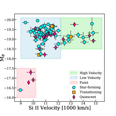
Figure 1: The peak $B$-band apparent magnitudes ($M_{B}$) vs Si II velocities with the uncertainties of 74 SNe from the Zheng et al. (2017) and Polin et al. (2021) samples. The SNe are colored by their hosts’ star formation classification: star-forming (blue circles), transitioning (yellow squares) and quiescent (red diamonds). High velocity SNe Ia ($\geq 12,200$ km/s) are outlined in the green box, low velocity SNe Ia in the blue box, and SN 1991bg-like faint SNe ($M_{B}>-17.5$ mag) are highlighted in the pink box. The entire population is dominated by star-forming galaxies ($\approx 67\%$), and the high and low velocity SNe Ia roughly follow those fractions ($\approx 64\%$ and $\approx 71\%$, respectively), while the faint SNe are almost entirely found in quiescent hosts.

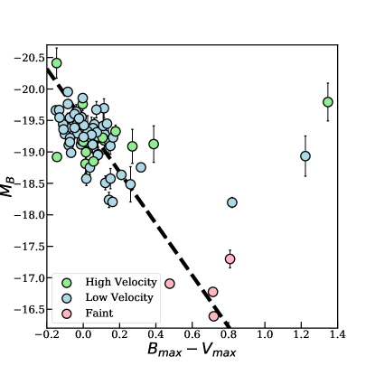
Figure 2: The peak $B$-band luminosities and $B-V$ colors for high velocity (green), low velocity (blue), and faint SNe (pink). The dashed black line shows the standard Milky Way dust extinction law with $R_{B}=4.1$. High velocity SNe Ia trend towards redder colors than low velocity SNe Ia.

2 Supernovae Sample

We conduct our host galaxy analysis based on the SNe Ia sample described in Zheng et al. (2017) and Zheng et al. (2018). This sample includes SNe discovered and observed by the Lick Observatory Supernovae Search (LOSS; Filippenko et al. 2001; Leaman et al. 2011), the Harvard Smithsonian Center for Astrophysics Data Release 3 (Hicken et al., 2009), and the Carnegie Supernova Project (Contreras et al., 2010). We note that these surveys are galaxy-targeted and can be constructed to be volume-limited. Their main advantage over other surveys is that they are able to detect faint SNe Ia several magnitudes below peak brightness, and thus can find SNe Ia that have a much smaller contrast with their hosts and/or suffer from local extinction. As the goal of this work is to better understand if faintness and redness in SNe Ia is correlated with host galaxy properties, this sample is preferred over the Palomar Transient Factory (PTF), Zwicky Transient Facility (ZTF), and other magnitude-limited surveys, which are naturally biased against detecting faint SNe or those with low contrast over their host(Frohmaier et al., 2017). These SNe were selected based on the conditions outlined in Zheng et al. (2017), which required SN discovery at 1 magnitude fainter in $B$-band than peak brightness and good photometric coverage post-discovery to properly model their lightcurves and estimate their peak luminosities. We include 53 out of the 56 total SNe in this sample based on the available SNe and host galaxy data (see Section 3.1). We additionally include 21 more SNe in Polin et al. (2021) and references therein that have public data in the Weizmann Interactive Supernova Data Repository (WISeREP; Yaron & Gal-Yam 2012) and the Open Supernovae Catalog (OSC; Guillochon et al. 2017). These SNe Ia have a peak spectrum and a nebular spectrum taken between $\approx$150–300 days, thus have comparable data to the Zheng et al. (2017) sample. All SNe Ia have spectroscopically confirmed redshifts that range between $0.0008<z<0.04$.

We divide the SNe sample into several categories based on the extinction-corrected peak $B$-band apparent magnitudes ($M_{B}$) and Si II velocities, determined in Zheng et al. (2018): high velocity SNe Ia (Si II velocities $>12,200$ km s^-1), low velocity SNe Ia ($<12,200$ km s^-1), and faint 1991bg-like (Filippenko et al., 1992) SNe ($M_{B}>-17.5$ mag), which we highlight in Figure 1. Given these sample divisions, we find that $\approx 18.9\%$ of the sample are high velocity SNe Ia, $\approx 75.6\%$ are low velocity SNe Ia, and $5.4\%$ are faint SNe. We note that only $\approx 2$ SNe overlap between high and low velocity SNe Ia samples given the uncertainties on the Si II velocities. As is shown in Figures 1 and 2, the high velocity SNe Ia appear to have a much narrower distribution of $M_{B}$ and Si II velocities than low velocity SNe Ia, with lower $M_{B}$, and redder colors. However, we note that choice of these sub-classes is not simply made from random cuts in $M_{B}$ and velocity space, as model-independent, statistical methods for dividing the SNe Ia sample has proven these sub-classes are clearly distinguished. For example, using a hierarchical cluster analysis, Benetti et al. (2005) observed a clear population difference between these three categories of SNe using ratios of the Si II lines. Burrow et al. (2020) further found these groups of SNe are distinguished between multiple photometric and spectroscopic properties of the SNe using Gaussian mixture models. As there is significant evidence that these SN sub-classes are separate and robust, we focus on the SN host environments to determine if we can use these properties to separate the SN classes and if they point to different progenitor or environmental differences that affect the SN observables, as has been suggested previously (Wang et al., 2009; Foley & Kasen, 2011; Wang et al., 2013; Polin et al., 2019; Pan, 2020; Pan et al., 2022).

3 Host Galaxy Observations & SED Modeling

3.1 Archival Data Collection

We determine host galaxies for each SN through querying nearby ($\lesssim 5\arcsec$) galaxies at approximately the same redshift as the SN via the the NASA/IPAC Extragalactic Database (NED). To model the host galaxies’ stellar population properties, we require broadband photometric observations in at least three different photometric filters covering at least two wavelength ranges (UV, optical, IR, and mid-IR), ensuring that the spectral energy distribution (SED) is well sampled. We collect archival photometric observations for all host galaxies via NED. We obtain UV, IR, and mid-IR observations through the GALEX (Bouquin et al., 2018), Two-Micron All Sky Survey (2MASS) (Skrutskie et al., 2006), and Wide-field Infrared Survey Explorer (WISE; Wright et al. 2010) surveys, respectively. Optical data is from the Sloan Digital Sky Survey (SDSS: $ugriz$; Ahumada et al. 2020) survey and and UBVRI data available on NED. We use photometry with similar aperture sizes for consistency in the SED fit, when possible. We correct all photometry for Galactic extinction in the directions of the SNe (Cardelli et al., 1989; Schlafly & Finkbeiner, 2011). Finally, we require impose a 5% error floor, forcing all uncertainties to be $\gtrsim 5\%$ the flux density value, to ensure that no photometric observation is overweighted in the stellar population modeling.

3.2 Stellar Population Modeling

To determine the stellar population properties of the SNe host galaxies, we use the stellar population modeling code Prospector (Leja et al., 2017; Johnson et al., 2021). We fit the observational data with Prospector through a nested sampling fitting routine, dynesty (Speagle, 2020), to return posterior distributions of the stellar population properties of interest. Prospector produces model SEDs with FSPS (Flexible Stellar Population Synthesis; Conroy et al. 2009; Conroy & Gunn 2010) using single stellar models through MIST (Paxton et al., 2018) and the MILES spectral library (Falcón-Barroso et al., 2011). The main fitted parameters are the age of the galaxy at the time of observation (the maximum allowed value is the age of the universe at the SN’s redshift), total mass formed, stellar metallicity ($Z_{*}$), and $V$-band optical depth.

For all Prospector fits, we use the Chabrier (2003) initial mass function (IMF) and a parametric delayed-$\tau$ star formation history (SFH $\propto te^{-t/\tau}$), defined by the $e$-folding time $\tau$, a sampled parameter. We include the effects nebular emission (Byler et al., 2017) and fix the gas phase metallicity ($Z_{\textrm{gas}}$) to solar since we do not use an observed spectrum in the modeling and therefore cannot measure spectral line strengths. We constrain the total mass formed and stellar metallicities through the Gallazzi et al. (2005) mass-metallicity relation to probe realistic masses for a given stellar metallicity. We measure dust attenuation through the Kriek & Conroy (2013) model, which includes a sampled parameter that determines the offset from the Calzetti et al. (2000) attenuation curve. Additionally, we allow the fraction of dust attenuated from young to that from old stellar light to be a sampled parameter to create more flexibility in determining the $V$-band optical depth, which hereafter we report as a $V$-band magnitude ($A_{V}$). As the majority of hosts have available 2MASS and WISE data, we include the Draine & Li (2007) IR dust emission model, a three-component dust emission model. To balance dimensionality in the model with the available photometry and ensure that that the model is not overfitting the data, we only sample one of the three components: the polycyclic aromatic hydrocarbon mass fraction ($q_{\textrm{pah}}$).

Table 1: Stellar Population Properties for SNe Host Samples

Sample	$t_{m}$ [Gyr]	log(M∗/M⊙)	SFR [M⊙/yr]	log(sSFR) [yr-1]	log(Z∗/Z⊙)	AV [mag]
High Velocity SNe	$3.14^{+6.63}_{-2.69}$	$10.09^{+0.66}_{-0.45}$	$0.59^{+6.39}_{-0.57}$	$-10.16^{+1.2}_{-2.3}$	$-0.83^{+1.0}_{-0.29}$	$0.58^{+0.83}_{-0.5}$
Low Velocity SNe	$1.26^{+4.83}_{-0.83}$	$9.99^{+0.65}_{-1.0}$	$0.51^{+4.86}_{-0.49}$	$-10.05^{+1.2}_{-2.34}$	$-0.75^{+0.75}_{-0.41}$	$0.57^{+1.5}_{-0.5}$
Faint SNe	$5.81^{+4.37}_{-4.37}$	$10.07^{+0.67}_{-0.55}$	$0.01^{+0.07}_{-0.01}$	$-11.96^{+1.36}_{-4.11}$	$-0.89^{+1.16}_{-0.27}$	$0.07^{+0.03}_{-0.05}$

Note. — The median and 68% credible interval for the Prospector-derived stellar population properties of the hosts of SNe divided into three categories: high velocity, low velocity, and faint SNe.

Finally, one host in this sample (SN 1998dm), shows significant evidence for an active galactic nuclei (AGN), given that the WISE w1 photometric observation is 1.29 mag greater than the WISE w2 photometric observation, a clear signal of AGN activity (Leja et al., 2018). Thus, we apply two AGN parameters to the fit of this host: the total luminosity of the AGN and the mid-IR optical depth. We follow the methods in Nugent et al. (2020) to calculate the stellar mass ($M_{*}$), present-day star formation rate (SFR), and mass-weighted age ($t_{m}$) for each host.

Finally, to classify each host by the degree of star formation, we use the definitions in Tacchella et al. (2022), which measures the combination of the specific SFR (sSFR = SFR/$M_{*}$; yr^-1) and the Hubble time $t_{\text{H}}(z)$ at the SN’s redshift: $\mathcal{D}(z)=\text{sSFR}\times t_{\text{H}}(z)$. If $\mathcal{D}(z)>1/3$, the host is classified as actively star-forming, if $\mathcal{D}(z)<1/20$ the host is quiescent (no active star formation), and if $1/20>\mathcal{D}(z)>1/3$, the host is transitioning from star forming to quiescent. We describe our main results from stellar population fitting in the following section.

4 Global Stellar Population Properties

Here, we discuss the results from the Prospector fitting of 74 SNe hosts. In Table 1, we list the median and 68% credible interval for the stellar population age, stellar mass, SFR, specific SFR, stellar metallicity, and $A_{V}$ for the different types of Ia SNe explored in this paper. We discuss correlations between the Prospector-derived stellar population properties in the following subsections.

4.1 Star Formation

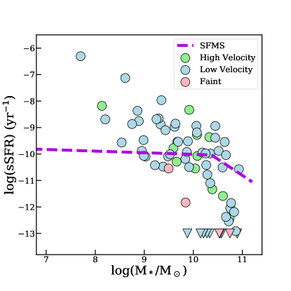
Figure 3: The sSFRs and stellar masses for the hosts of SNe divided into three categories: high velocity (green), low velocity (blue), and faint SNe (pink). Downward arrows represent upper limits. We find that both high and low velocity explosions trace the SFMS (purple line; Leja et al. 2022) and similar galaxies with relation to the amount of star formation and stellar mass, however the faint SNe are exclusively found in larger and lower-sSFR galaxies.

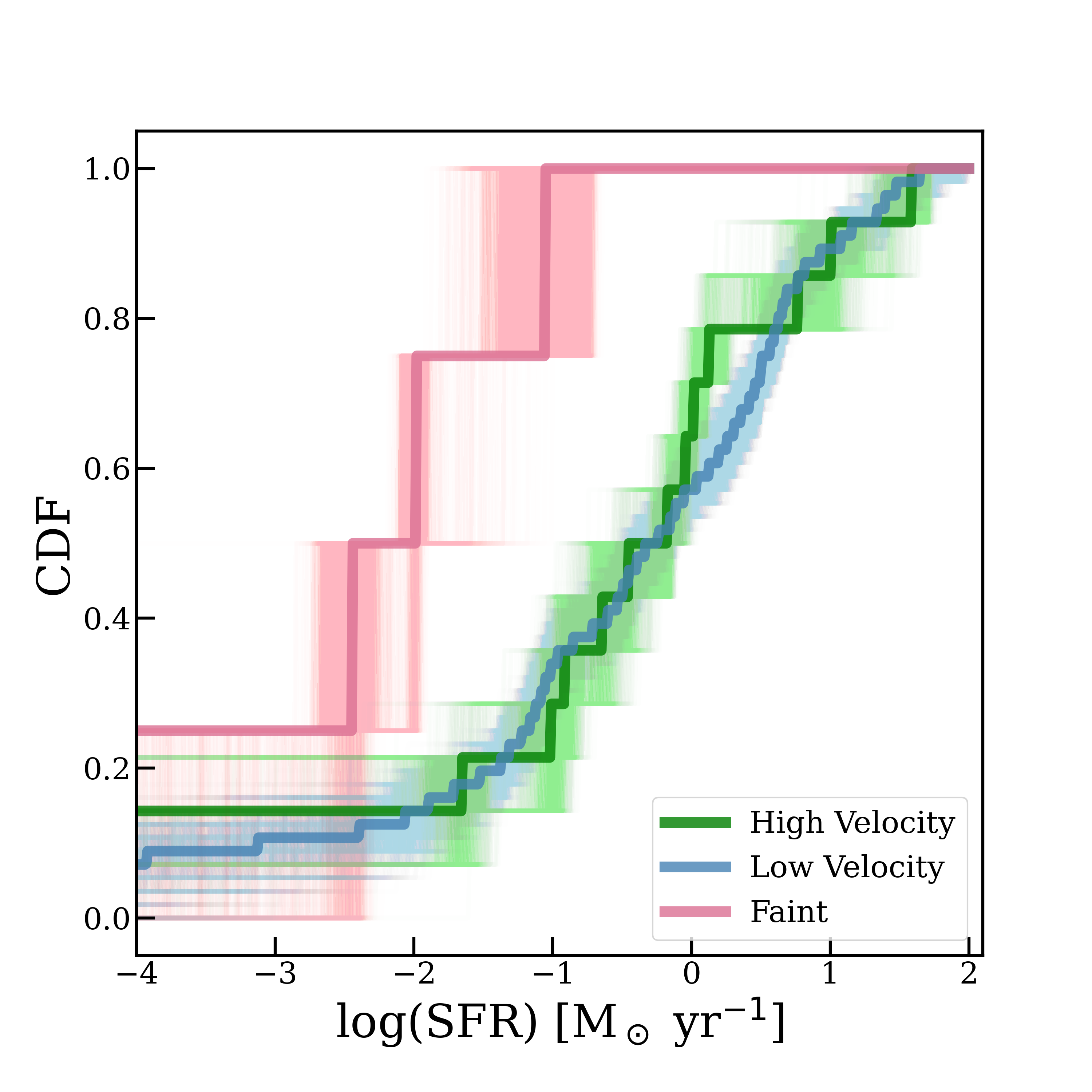
Figure 4: The cumulative distribution (CDF) and 5000 realizations on the CDF for the SFRs of high velocity (green), low velocity (blue), and faint SNe (pink) hosts. The darker color line represents the median of the CDFs. When comparing the CDFs, we find no evidence that high and low velocity SNe Ia derive from different host galaxies with respect to SFR. The faint SNe hosts, on the other hand, have much lower SFRs, suggesting their progenitor is likely less dependent on star formation than those of the other two SNe categories.

We first focus on the global star formation properties of the host galaxies to determine if the SN type is related to star formation activity. We highlight the SNe categories with respect to their peak $M_{B}$ and Si II velocities along with their hosts’ star formation classification in Figure 1. We find that $\approx 67.6\%$ of the entire SNe host population are star-forming galaxies, with $\approx 28.3\%$ quiescent galaxies, and $\approx 4.1\%$ transitioning. This roughly follows the star-forming fraction of the observed Type Ia SNe host population (Mannucci et al., 2008) The high and low velocity SNe Ia hosts roughly follow these fractions: high velocity SNe Ia hosts are 64.2% star-forming, 7.1% transitioning, and 28.6% quiescent, while low velocity SNe Ia hosts are 71.4% star-forming, 3.5% transitioning, and 25.0% quiescent. The faint SNe hosts are almost solely quiescent galaxies (75% quiescent, 25% star-forming). To test whether the host populations of high and low velocity SNe Ia are statistically different, we randomly draw 14 and 56 hosts (the number of high and low velocity SNe Ia hosts, respectively) from the entire population 10,000 times, and determine the median and 1$\sigma$ star-forming fractions. We find that when drawing the number of high velocity SNe Ia hosts, we derive a star-forming fraction of 64$\pm 12\%$ and while drawing the number of low velocity SNe Ia hosts, we find a star-forming fraction of $67\pm 6\%$. Thus, we determine that the respective star-forming fractions of the high and low velocity SNe Ia hosts are consistent to each other with the general population to within $1\sigma$.

We further analyze the hosts by comparing their specific star formation rates (sSFRs) versus stellar mass. We compare how these properties trace the star-forming main sequence (SFMS), a well-studied galaxy relation that tracks the SFRs of star-forming galaxies as they gain stellar mass (Whitaker et al., 2014; Speagle et al., 2014; Leja et al., 2022). How transient hosts track the SFMS has important implications for the environmental conditions their progenitor traces (e.g. dependencies on bursts of star formation or the amount of stellar mass). In Figure 3, we plot the sSFRs and stellar masses of the SNe hosts in each of the three categories, along with the SFMS derived in Leja et al. (2022) for $z<0.5$. This SFMS was derived from a population of galaxies in the COSMOS-2015 and 3D-HST surveys with stellar population modeling fitting from Prospector, thus is comparable to our results (Leja et al., 2022). We choose to use the sSFR as opposed to the SFR, as it normalizes the amount of star formation per stellar mass unit, which is useful when comparing galaxies across large stellar mass ranges. We find that both the high and low velocity SNe Ia hosts trace the SFMS well, and are not clustered into any particular combination of sSFR and stellar mass. The faint SNe, on the other hand, are exclusively found in high stellar mass hosts with low sSFRs. This suggests that while the faint SNe progenitor is more apparently connected to stellar mass rather than star formation (and therefore likely has an older stellar progenitor), the high and low velocity progenitors depend on a wider array of environmental factors, suggesting a breadth of possible environments and progenitor timescales with similar dependencies on star formation and stellar mass.

We next compare cumulative distribution functions (CDFs) of SFR between the three categories of SNe and their hosts. We build the CDFs by randomly drawing 5000 values from each host’s Prospector-derived posterior distribution for each property. We then build 5000 CDFs for each SN category, as shown in Figure 4. We compare all CDFs through an Anderson-Darling (AD) test, with the null hypothesis that the hosts are all derived from the same SFR distribution, and calculate the percentage of tests with a probability $P_{AD}<0.05$, the point at which we can reject the null hypothesis and list these values in Table 2. We find that when comparing the SFRs of high and low velocity SNe Ia hosts, $0\%$ of AD tests result in a rejection of the null hypothesis, with the same result being found when comparing sSFRs. We thus infer that if the high and low velocity SNe Ia Ia represent different progenitors, neither progenitor is more dependent on the amount of recent star formation in their environment and thus, the amount of global star formation in a host cannot be used to distinguish these SN populations. Meanwhile, the null hypothesis can be rejected in $76.5\%$ ($86.5\%$) and $94.7\%$ ($96.6\%$) of the SFR (sSFR) tests for the faint SNe and high velocity SNe Ia hosts and faint SNe and low velocity SNe Ia hosts, respectively. This implies that that the faint SNe progenitor is less dependent on recent star formation than either the high or low velocity SNe Ia.

Table 2: Anderson Darling Testing Results

Sample	$t_{m}$	log(M∗/M⊙)	SFR	sSFR	log(Z∗/Z⊙)	AV	Offset	Na I D
High & Low Velocity SNe	0.0%	0.0%	0.0%	0.0%	0.0%	0.0%	$0.003$	26.9%
High Velocity & Faint SNe	0.0%	0.0%	76.5%	86.5%	0.0%	80.9%	$0.22$	53.3%
Low Velocity & Faint SNe	18.2%	0.0%	94.7%	96.6%	0.0%	98.9%	$>0.25$	13.1%

Note. — The results of Anderson Darling testing of the stellar population properties, offsets, and Na I D equivalent widths for pairs of SNe types in this study (high and low velocity SNe, high velocity and faint SNe, and low velocity and faint SNe). We list the percentage of the 5000 tests run that reject the null hypothesis ($P_{AD}<0.05$) for the stellar population properties and Na I D equivalent widths. We list the $P_{AD}$ values for the offsets as there are no uncertainties.

Overall, these results point to the fact that we cannot separate high and low velocity SNe Ia from the amount of global star formation in their hosts, although we note that locally they may indeed trace different star formations.

4.2 Stellar Mass, Age, Metallicity, and Dust

We next compare the main stellar population properties (stellar mass, stellar metallicity, stellar age, total dust) of each SN group’s hosts. We show the $M_{B}$ vs. Si II velocity relation of the SNe colored by the median stellar mass, stellar population age, stellar metallicity, and dust from the Prospector posterior distributions of their hosts in Figure 5. We list the derived median and 68% credible interval for each SN category in Table 1. We find that there is very little difference in stellar population property compared to SN type. However, as the faint SNe are almost exclusively in non-star forming hosts, they reside in older galaxies with lower dust and higher stellar mass than the hosts of the other SN types. Furthermore, we see little evidence that the peak $B$-band luminosity and Si II velocities are correlated at all with host galaxy stellar population properties.

In Figure 6, we compare the CDFs of each stellar population property for the three SN categories (see Section 2) and compare the distributions through AD tests, results of which are listed in Table 2. We cannot reject the null hypothesis for any of our comparisons in stellar mass and stellar metallicity. This implies that all SNe originate from galaxies with the same underlying stellar mass and stellar metallicity distributions. The similarities in the stellar mass distributions between high and low velocity SNe Ia hosts contradicts the conclusion found in Pan (2020), in which all high velocity SNe Ia (defined as having Si II velocities $>12,000$ km s^-1, at $z<0.19$ were found in galaxies with $>10^{9.6}M_{\odot}$ and preferentially occurred in more massive galaxies than low velocity SNe Ia. In this work, we find one high velocity SN Ia host lower than this stellar mass minimum, at $\approx 10^{8.1}M_{\odot}$ (the host of SN 2007qe, which was not included in the Pan 2020 sample), thus this is likely driving the stellar mass distributions to be more similar. We also note that the stellar mass estimates determined in this work are all $\approx 0.3$ dex smaller than the masses determined in Pan (2020) between the 10 shared hosts, which is a known effect when switching from a Salpeter IMF (used in Pan 2020) to a Chabrier IMF (this work). However, most importantly, the difference will only affect individual stellar mass measurements and not how the distributions of stellar masses compare. Thus, the similarity of the stellar mass distributions between high and low velocity SNe Ia found in this work is real, and not simply caused by a different stellar population modeling technique or SED fitting tool. Moreover, this implies that high velocity SNe Ia can occur in a more diverse array of environments than previously known.

For mass-weighted age, we can reject $0\%$ of tests between high and low velocity SNe Ia hosts and $18.2\%$ of tests between low velocity and faint SNe hosts. The null hypothesis cannot be rejected in any of the trials between high velocity and faint SNe hosts. This indicates the age distributions are fairly similar across all three SNe host categories. However faint SNe hosts lack $\lesssim 1$ Gyr hosts, given their more substantial presence in older, quiescent galaxies. As shown in Figure 6, we find that the stellar population ages of high velocity SNe Ia hosts veer toward older ages than low velocity SNe Ia hosts, likely causing their age distributions to be more similar to those of faint SNe hosts than low velocity SNe Ia are to faint SNe hosts, and may be suggestive of a slightly older progenitor with a longer delay time. This conclusion is in agreement with the analysis conducted in Pan (2020) and Pan et al. (2022), wherein high velocity SNe Ia trended toward lower redshift and more metal-rich (from gas-phase metallicities not the stellar metallicities studied here) environments than low velocity SNe Ia, suggesting that the high velocity SNe Ia progenitor prefers longer delay times. Furthermore, we find that $0\%$ of tests can be rejected between $A_{V}$ distributions between the high and low velocity SNe Ia hosts. However, as the faint SNe hosts tend to have very little dust, we find that $80.9\%$ of AD tests can be rejected between faint SNe and high velocity SNe Ia host $A_{V}$ distributions, and $98.9\%$ of tests can be rejected between faint SNe and low velocity SNe Ia host $A_{V}$ distributions.

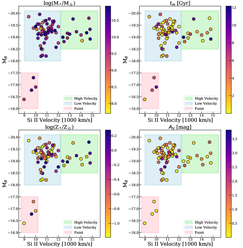
Figure 5: The same plot as in Figure 1, with SNe colored by their hosts’ amount of stellar mass (log($M/M_{\odot}$), top left), mass-weighted age ($t_{m}$, top right), stellar metallicity (log($Z_{*}/Z_{\odot}$), bottom left), and total $A_{V}$ (bottom right). We find that there appears very little correlation between host stellar population property and SN property.

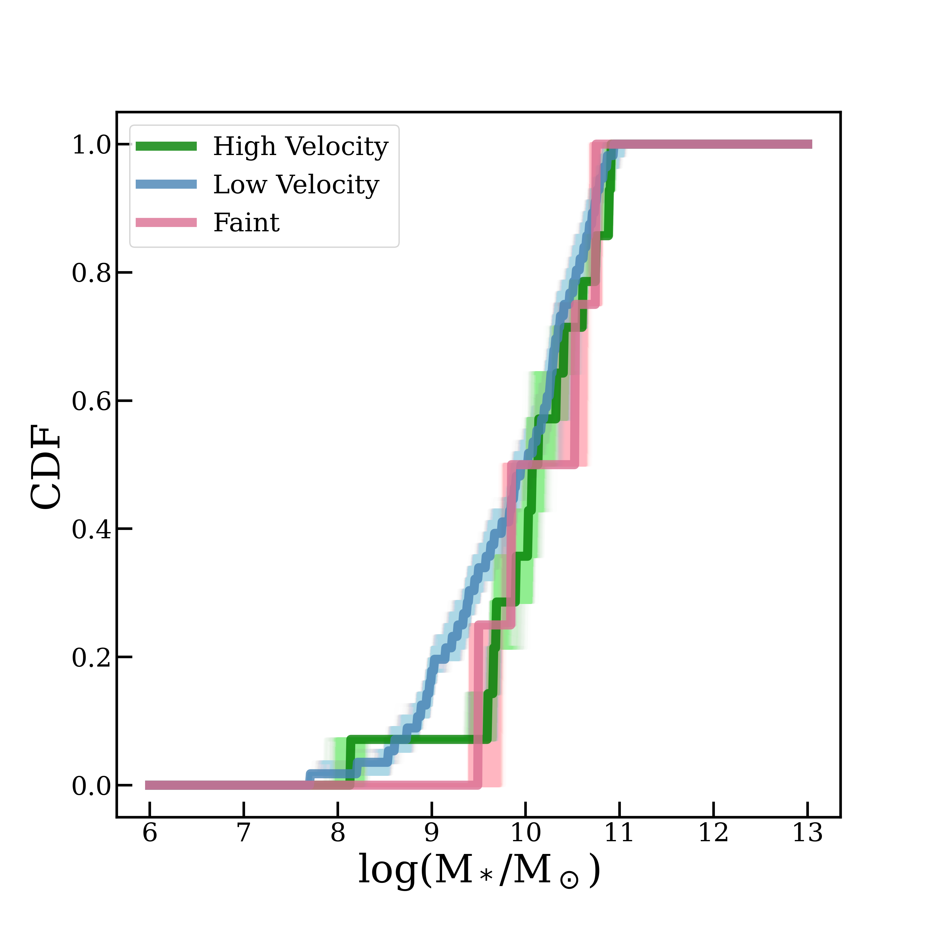
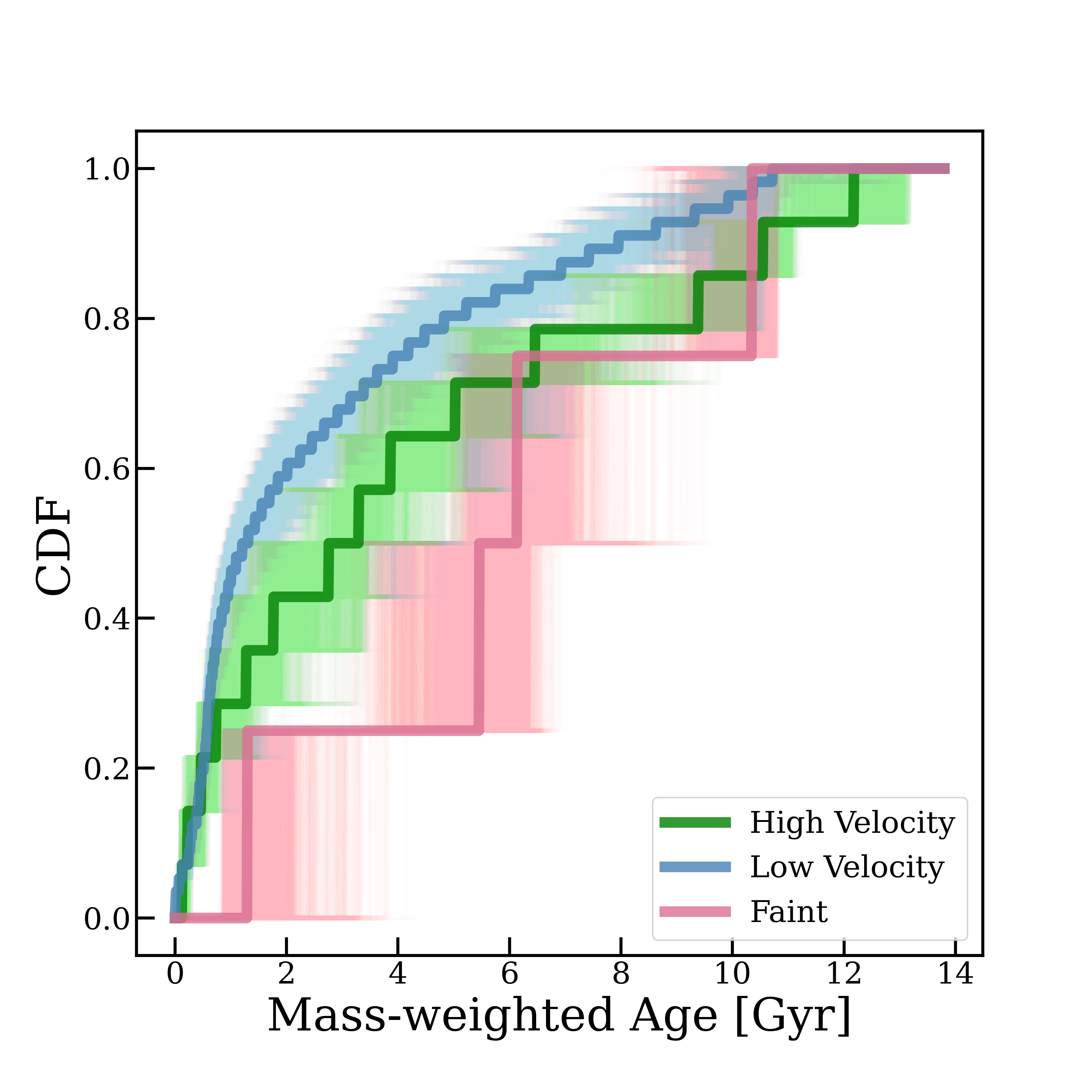
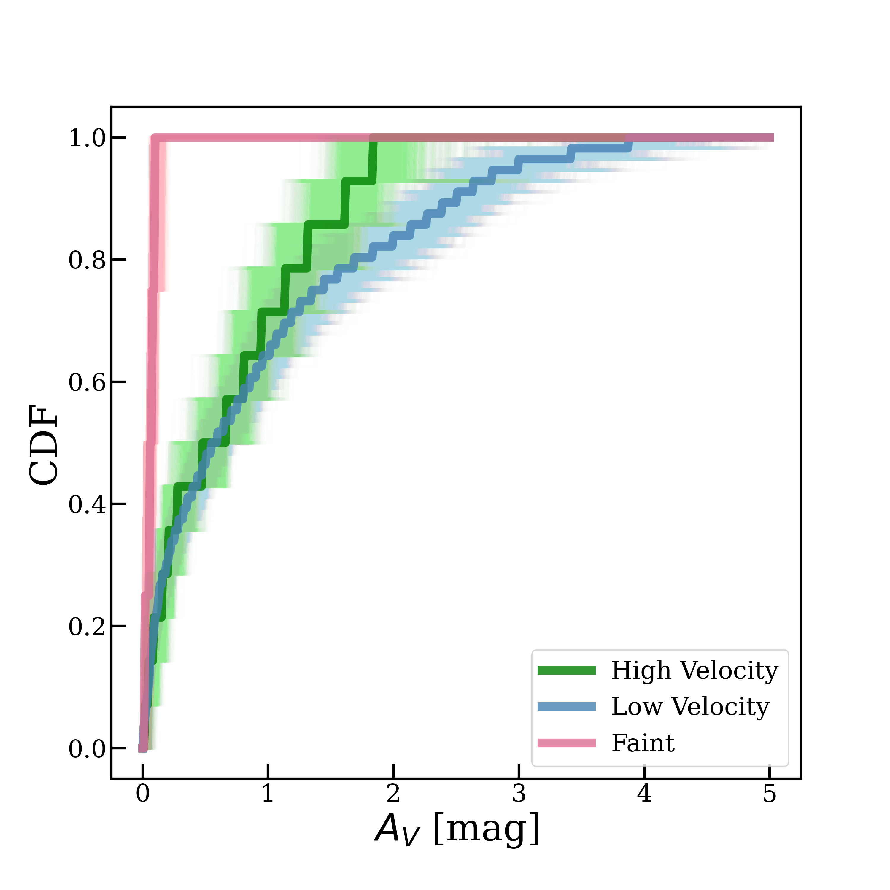
Figure 6: From left to right, top to bottom: CDFs of stellar mass (log($M/M_{\odot}$)), mass-weighted age, stellar metallicity (log($Z_{*}/Z_{\odot}$)), and total $A_{V}$ for the three categories of SNe: high velocity (green), low velocity (blue), and faint SNe (pink), with darker colors representing the median CDF. We find that there is very little difference in stellar population properties between the high and low velocity SNe Ia hosts, suggesting that global host properties alone cannot be used to separate these SN classes or distinguish different progenitor types. The faint SNe host galaxies are much older and less dusty, suggesting they may derive from an older stellar progenitor.

Overall, we find very little evidence for significant stellar population property difference between high and low velocity SNe Ia populations, suggesting the global environment alone cannot distinguish the two SNe and that their progenitors’ environments have similar stellar population properties. Furthermore, this suggests that the differences in SN properties of either group cannot be explained by differences in their global host environments. We find more substantial evidence that the environments of faint SNe are quite different, however note that the population of faint SNe we have explored in this paper is quite small thus might not be fully representative of the host properties of all faint SNe.

5 Evidence for Difference in Local Environments

As discussed in the previous section, we find little evidence that the global environmental properties of possible high and low velocity SNe are different. In this section, we discuss if their progenitors are tracing different local environments through analyzing their observed physical offset distributions and Na I D equivalent widths.

5.1 Offsets

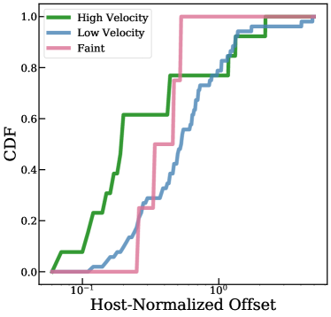
Figure 7: CDFs of the host-normalized offsets for the high velocity (green), low velocity (blue), and faint SNe (pink) classifications. High velocity SNe Ia have smaller host-normalized offsets than either low velocity of faint SNe, implying they lie more towards the center of their hosts than the other SN sub-classes. As more star formation lies towards the center of galaxies, this may suggest that high velocity SNe Ia have a progenitor more connected to or observables that are more affected by recent star formation in their local environments than low velocity or faint SNe.

The offsets of transients from the center of their host galaxies has been used to connect their progenitors to recent star formation and their migration from their birthplace, as it is assumed that the majority of star formation activity lies, and therefore more stars are born, towards the center of galaxies (e.g. Kasliwal et al. 2012; Blanchard et al. 2016; Fong et al. 2022). Thus, the relative offset distributions between transients can be used to distinguish progenitor systems. We obtain angular separations of our SNe sample to the center of their hosts and the 2MASS K-band “total” radii of the host galaxies, which is available for 69 out of the 74 host studied in this work (13/14 high velocity SNe Ia and 52/56 of the low velocity SNe Ia hosts) from NED. We determine host-normalized offsets, or the relative location of the SN within its host, by dividing the angular separation of each SNe to their hosts’ centers by the host galaxies’ size. We find that high velocity SNe Ia have host-normalized offsets $0.19^{+0.99}_{-0.08}$ $r/r_{e}$, low velocity SNe Ia hosts have offsets $0.53^{+0.61}_{-0.29}$ $r/r_{e}$, and faint SNe have offsets $0.4^{+0.1}_{-0.11}$ $r/r_{e}$, and we show the respective CDFs in Figure 7. When conducting an AD test between pairs of the three SNe offset distributions, we find that we cannot reject the null hypothesis for any pair ($P_{AD}\geq 0.20$) except the high and low velocity SNe Ia ($P_{AD}=0.003$), as high velocity SNe Ia appear to be more concentrated towards the center of their hosts than low velocity SNe Ia. These results are in agreement with those in Wang et al. (2013), which studied the relative locations of high and low velocity SNe Ia within their hosts, finding high velocity SNe Ia occur at lower radial distances. Assuming that more star formation lies towards the center of galaxies, this could imply that the high velocity SNe Ia progenitor is more connected to recent star formation than the low velocity SNe Ia progenitor and thus may trend towards younger delay times, which interestingly does not correlate with the implications in Pan (2020) and Pan et al. (2022), where it was proposed that the high velocity SN Ia progenitor may have a longer delay time than that of low velocity SNe Ia. Furthermore, this could indicate that high velocity SNe Ia appear redder from extinction in their local environments, as more gas and dust lies towards the center of the galaxies. Overall, these results highlight that while global properties of high and low velocity SNe Ia may not be distinguished, the local environments may play a larger role in separating these sub-classes.

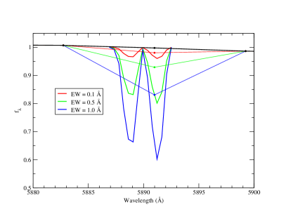
Figure 8: An example measurement of the equivalent width on the day $+$4 spectrum of SN 1990N (Leibundgut et al., 1991) seen in black. An upper limit of 0.1 Å can be placed on this individual spectrum. We present example strengths of the lines at 0.1, 0.5 and 1.0 Å in both high-resolution and at the resolution these Na I D lines would have in the lower resolution of the observed spectrum (in red, green, and blue respectively)

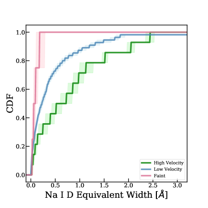
Figure 9: CDFs on the Na I D line equivalent widths for high velocity (green), low velocity (blue), and faint (pink) SNe. Darker lines represent the median of the distribution and lighter lines represent uncertainty on the CDF. We find that high velocity SNe Ia tend to have stronger Na I D equivalent widths than low velocity SNe Ia, implying either their interstellar or circumstellar environments contain more Na gas.

5.2 Na I D Equivalent Widths

Finally, we analyze the equivalent widths of the Na I D lines in each SN spectrum to infer if high and low velocity SNe Ia probe different circumstellar or interstellar environments. The Na I D line strength probes the host dust and circumstellar gas, dust, and metals (Blondin et al., 2009; Folatelli et al., 2010; Poznanski et al., 2012; Phillips et al., 2013), thus is a good indicator of the local environment surrounding the SN (Sternberg et al., 2011a, 2014). We collect published Na I D equivalent widths for 61 SNe in Wang et al. (2019) and references therein. For the 13 remaining SNe: 1990N (Jeffery et al., 1992; Gómez & López, 1998), 1991bg (Filippenko et al., 1992), 2005hk (Phillips et al., 2007), 2000E, 2006ax, 2006lf, 2008Q (Blondin et al., 2012), 2000dr, 2002cs, 2003Y, 2003gn, 2003gt, 2007on (Silverman et al., 2012), we collect spectra from WISeREP (Yaron & Gal-Yam, 2012). To determine the Na I D equivalent widths for these SNe Ia, we performed a standard equivalent width measurement on these mostly lower resolution spectra as seen in Figure 8. In the case where a SN has multiple high signal-to-noise spectra, we measured the equivalent width on each spectrum and added them statistically. We note that in all but two cases (SNe 2006lf and 2007on), they are upper limits. We find that high velocity SNe Ia have Na I D equivalent widths $0.62^{+0.95}_{-0.55}$ Å, low velocity SNe Ia have equivalent widths $0.22^{+0.61}_{-0.19}$ Å, and faint SNe have equivalent widths $0.07^{+0.09}_{-0.05}$ Å.

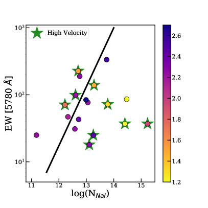
Figure 10: A plot of the equivalent width of the 5780 Å DIB vs. column depth of Na I for those SNe Ia from Phillips et al. (2013) that we can separate between low and high velocity. While all but one of the low velocity SNe Ia tightly follow the correlation found in the Milky Way galaxy (black line), nearly half the high velocity SNe Ia fall outside this correlation. We have color coded the data points by their assumed $R_{V}$.

To make CDFs of the Na I D equivalent widths, we build Gaussian distributions using their median and $1\sigma$ uncertainties, with a minimum possible value of 0 Å, and sample from this distribution 5000 times. We show the median and 68% credible interval for these CDFs in Figure 9. We compare pairs of the 5000 CDFs and list the percentage of tests that reject the null hypothesis in Table 2. We find that we can reject the null hypothesis in 26.9% of the tests between high and low velocity SNe Ia, 53.3% of tests between high velocity and faint SNe, and 13.1% of tests between low velocity and faint SNe. We see in Figure 9, that high velocity SNe Ia have larger Na I D equivalent widths than low velocity SNe Ia, implying that their circumstellar environments likely have higher amounts of Na I gas caused either by properties intrinsic to the progenitor and SN or, as was observed with the offsets in Section 5.1, by larger amounts of Na I gas along the line of sight through the host galaxy.

6 Discussion

In this work, we have focused on the global host galaxy and local environmental properties of high and low velocity SNe Ia to see if we can find evidence for a separate progenitor system or environmental condition that could explain why high velocity SNe Ia appear redder. While we find no evidence that the global host properties can account for these differences in SN observables, we have shown that more locally, using the host normalized offsets and Na I D equivalent widths, high and low velocity SNe Ia may indeed differ. However, understanding the contribution of the local environmental properties versus the progenitor properties to the redness of high velocity SNe Ia requires discerning whether the excess Na I D gas observed in high velocity SNe comes from the circumstellar or interstellar medium. Indeed, Phillips et al. (2013), which explored the properties of SNe Ia as a function of both the diffuse interstellar bands (DIBs) and Na I D lines through high-resolution spectroscopy, found that (i) the low $R_{V}$ values derived for very reddened SNe Ia are likely caused by dust in the interstellar medium, and not the circumstellar medium, and (ii) that nearly a quarter of SNe Ia have large host Na I column densities in comparison with the amount of dust observed to redden their spectra. Phillips et al. (2013) further noted that all of the SNe Ia with unusually strong Na I D lines have “blueshifted” profiles in the classification scheme following (Sternberg et al., 2011b) and that the majority of the high velocity SNe Ia (seven out of ten) have this “blueshifted” feature. This paper, however, relies on one major assumption: that the intrinsic colors of both the high and low velocity SNe Ia are similar as defined by the SNooPy algorithm (Burns et al., 2011). Here, we revisit these conclusions given more recent work on the potential origins of these two sub-groups of SNe Ia.

One theory for the origins of high velocity SNe Ia are that they derive from a separate progenitor than low velocity SNe Ia. For example, Polin et al. (2019) suggests that the high velocities and redder colors of high velocity SNe Ia are a natural consequence of a sub-$M_{\textrm{ch}}$ mass explosion. Current sub-$M_{\textrm{ch}}$ explosion models predict greater ⁵⁶Ni production than in classical $M_{\textrm{ch}}$ explosions and, combined with the excess nucleosynthesis occurring in the outer layers, will result in these SNe Ia being redder as well (Shen et al., 2018; Polin et al., 2019). Due to this excess in ⁵⁶Ni production, Polin et al. (2019) predicts that there exists a tight relationship between the mass of the white dwarf and the kinetic energy of the explosion, which can be translated to a tight relation between the observed peak SN luminosities and Si II velocities (Figure 11, Polin et al. 2019), which will not be followed by $M_{\textrm{ch}}$ explosions. As high velocity SNe Ia trace the Polin et al. (2019) sub-$M_{\textrm{ch}}$ model peak luminosity — Si II velocity relation well, and furthermore have just as red if not redder peak $B-V$ colors than the models (Figure 12, Polin et al. 2019), this suggests that high velocity are likely sub-$M_{\textrm{ch}}$ mass explosions. Many of the low velocity SNe Ia, on the other hand, are much bluer than the Polin et al. (2019) sub-$M_{\textrm{ch}}$ models and have peak luminosities that are too high for their Si II velocities. Thus, these suggest that they are likely a different explosion mechanism, perhaps being $M_{\textrm{ch}}$ explosions. We note that while others claim that the bulk of the low velocity SNe Ia can also derive from sub-$M_{\textrm{ch}}$ explosions (Shen et al., 2021), we use the Polin et al. (2019) model to guide our discussion and simply note that this relationship implies that we are seeing at least two separate progenitor systems and/or explosion mechanisms.

If high and low velocity SNe Ia do indeed derive from these separate progenitor systems, it implies that the colors of these two groups are intrinsically different, which affects the interpretation of the Phillips et al. (2013) conclusions. While it is unknown what the true colors of high velocity SNe Ia are, assuming they are derived from the Polin et al. (2019) sub-$M_{\textrm{Ch}}$ explosion model, it does imply that they are redder than the assumption made by Phillips et al. (2013) in their interpretation of the extinction. Nonetheless, this only strengthens the findings in Phillips et al. (2013) as the anomalously low values of $R_{V}$ they found for reddened SNe Ia would become even lower and the lack of correlation between the strength of the Na I D lines and the DIBs, or assumed dust from the underlying colors, would become even smaller. An example of this can be seen in Figure 10. Here, we have plotted the equivalent width of the 5780 Å DIB versus column depth of Na I for those SNe Ia from Phillips et al. (2013) that we can separate between low and high velocity. While all but one of the low velocity SNe Ia tightly follow the correlation found in the Milky Way galaxy, nearly half the high velocity SNe Ia lie outside this correlation. Such a result strongly implies that, as Phillips et al. (2013) noted, the dust is a property of the ISM and furthermore that the CSM of these events is almost certainly contributing a clear excess to the Na I D profiles as first noted by Maguire et al. (2013). Here they saw that those SNe Ia with blueshifted Na I D profiles had both an excess absorption compared to those with non-blueshifted profiles and redder $B-V$ colors at peak brightness.

While we have only considered three sub-groups of SNe Ia with simple velocity and peak brightness cuts, we note that the sub-$M_{\textrm{ch}}$ models of Polin et al. (2019) extend down to more normal velocities (v $\sim 10,750$ km/s) and slightly fainter peak absolute magnitudes (B $\sim-18.5$). It would be interesting to see in a future, larger, volume limited, sample if the blueshifted SNe Ia noted by Maguire et al. (2013) and Phillips et al. (2013) shared the characteristics of this sub-population of SNe Ia. Additional future work is also needed to understand how the more local environments of these sub-$M_{\textrm{Ch}}$ explosion candidates may further affect their colors and SN observables, as we have noted how high velocity SNe Ia trend towards smaller offsets from their hosts’ centers and are thus likely more observationally affected by extinction from star formation in these regions.

7 Conclusions

In this study, we have determined the host galaxy stellar population properties for 74 SNe Ia at $z<0.04$, divided into the sub-categories of high velocity, low velocity, and faint SNe Ia based on their peak $B$-band luminosities and Si II velocities. All SNe Ia have good photometric coverage for determination of their properties and their host galaxies have at least three bands of archival photometry, the minimum requirement for a stellar population fit. We summarize our main conclusions below:

• We find that there is no statistical evidence for differences between the high velocity (Si II velocities $\gtrsim 12,200$ km s^-1) and low velocity SNe Ia host galaxy populations in SFR, sSFR, stellar mass, stellar population age, dust attenuation, and stellar metallicity. The fainter ($M_{B}>-17.5$ mag) SNe occur almost exclusively in older, more massive, and more quiescent galaxies than the rest SNe population, and thus their overall host properties are quite distinguished from the high and low velocity SNe Ia hosts.

• In our comparison between the host-normalized offsets for the SNe (from SN position to center of the host), we find high velocity SNe Ia are more concentrated towards the center of their hosts than low velocity SNe Ia. This suggests that the high velocity SN Ia progenitor may be more connected to recent star formation and that their redder colors may in part be caused by extinction in their local environments.

• Finally, we find that high velocity SNe Ia have higher Na I D equivalent widths than low velocity SNe Ia. Given the results of Phillips et al. (2013), and assuming a sub-$M_{\textrm{ch}}$ origin for the high-velocity SNe Ia, this implies that origin of the excess absorption is in the CSM and is related to the progenitor system for the high velocity events.

Our results on the stellar population properties of SNe Ia hosts strongly suggest that the global environments of high and low velocity SNe Ia are not intrinsically different, however, we do find evidence that there may be more circumstellar or local environmental differences. Furthermore, the smaller host-normalized offsets of high velocity SNe Ia might imply that their progenitor is younger and more connected to recent star formation than that of low velocity SNe Ia. As it has already been proposed that sub-$M_{\textrm{ch}}$ progenitors are likely more connected to star formation and occur in younger stellar population than classical SNe Ia (de los Reyes et al., 2020), this further backs the sub-$M_{\textrm{ch}}$ progenitor system interpretation for the high velocity SNe Ia given the observational differences seen in Phillips et al. (2013) and theoretical properties for these events seen in Polin et al. (2019).

Future work necessitates the use of high-resolution photomotery and/or Integral Field Unit (IFU) spectroscopy to resolve the local environments of nearby high velocity SNe Ia to more conclusively determine if they trace separate environmental properties than more normal velocity SNe Ia and more conclusively inform if the excess Na I D gas in high velocity SNe Ia is interstellar or circumstellar. Indeed, Rigault et al. (2020) has already shown that the local star formation activity surrounding SNe Ia does affect the corrections to their peak magnitudes used in the standardization process for cosmology.

Our conclusions notably highlight that the global stellar population properties cannot be used to separate classes of SNe Ia for future cosmology measurements. This is especially problematic for the upcoming era of the Vera Rubin Observatory (VRO), in which hundreds of thousands of SNe Ia will be discovered, the majority of which will not be followed up with spectroscopy of the supernova to determine their Si II velocities. Furthermore, if the local environments of high-velocity SNe are indeed tracing younger, more star forming environments, then these environmental differences may only be probed for more local universe events where resolving stellar populations within a galaxy is possible. At higher redshift, where the majority of SNe will be discovered, such observations are not feasible. This, in effect, would lead to more contamination from these events in the population used for cosmology.

As separating SNe Ia by their global and/or local stellar population properties is extremely difficult, if not impossible, and obtaining a spectrum for the majority of SNe discovered by the VRO is too ambitious, a more concerted effort needs to be placed on distinguishing SNe Ia based on their photometric properties. Indeed, most current methods using SNe Ia as probes for cosmology impose a color cut using SALT2 of $|c|\lesssim 0.3$ (similar to a cut in $B-V$; Smith et al. 2020; Popovic et al. 2021). As strong Na I D lines imply redder SN, either due to actual extinction or association with the intrinsically redder sub-group of high-velocity SNe Ia, we can use this knowledge to make more informed color cuts such that high velocity SNe Ia are not included in the cosmology sample. Furthermore, if future analyses find that the ”blueshifted” Na I D subset of SNe Ia include both the high and lower velocity SNe Ia that follow the Polin et al. (2019) Si II velocity versus peak brightness relationship, then slightly more complicated cuts will be required.

References

- Ahumada et al. (2020) Ahumada, R., Prieto, C. A., Almeida, A., et al. 2020, ApJS, 249, 3, doi: 10.3847/1538-4365/ab929e
- Benetti et al. (2005) Benetti, S., Cappellaro, E., Mazzali, P. A., et al. 2005, ApJ, 623, 1011, doi: 10.1086/428608
- Bennett et al. (2014) Bennett, C. L., Larson, D., Weiland, J. L., & Hinshaw, G. 2014, ApJ, 794, 135, doi: 10.1088/0004-637X/794/2/135
- Blanchard et al. (2016) Blanchard, P. K., Berger, E., & Fong, W.-f. 2016, ApJ, 817, 144, doi: 10.3847/0004-637X/817/2/144
- Blondin et al. (2009) Blondin, S., Prieto, J. L., Patat, F., et al. 2009, ApJ, 693, 207, doi: 10.1088/0004-637X/693/1/207
- Blondin et al. (2012) Blondin, S., Matheson, T., Kirshner, R. P., et al. 2012, AJ, 143, 126, doi: 10.1088/0004-6256/143/5/126
- Bouquin et al. (2018) Bouquin, A. Y. K., Gil de Paz, A., Muñoz-Mateos, J. C., et al. 2018, ApJS, 234, 18, doi: 10.3847/1538-4365/aaa384
- Brout & Scolnic (2021) Brout, D., & Scolnic, D. 2021, ApJ, 909, 26, doi: 10.3847/1538-4357/abd69b
- Bulla et al. (2020) Bulla, M., Miller, A. A., Yao, Y., et al. 2020, ApJ, 902, 48, doi: 10.3847/1538-4357/abb13c
- Burns et al. (2011) Burns, C. R., Stritzinger, M., Phillips, M. M., et al. 2011, AJ, 141, 19, doi: 10.1088/0004-6256/141/1/19
- Burrow et al. (2020) Burrow, A., Baron, E., Ashall, C., et al. 2020, ApJ, 901, 154, doi: 10.3847/1538-4357/abafa2
- Byler et al. (2017) Byler, N., Dalcanton, J. J., Conroy, C., & Johnson, B. D. 2017, ApJ, 840, 44, doi: 10.3847/1538-4357/aa6c66
- Calzetti et al. (2000) Calzetti, D., Armus, L., Bohlin, R. C., et al. 2000, ApJ, 533, 682, doi: 10.1086/308692
- Cardelli et al. (1989) Cardelli, J. A., Clayton, G. C., & Mathis, J. S. 1989, ApJ, 345, 245, doi: 10.1086/167900
- Chabrier (2003) Chabrier, G. 2003, PASP, 115, 763, doi: 10.1086/376392
- Childress et al. (2013) Childress, M., Aldering, G., Antilogus, P., et al. 2013, ApJ, 770, 108, doi: 10.1088/0004-637X/770/2/108
- Conroy & Gunn (2010) Conroy, C., & Gunn, J. E. 2010, ApJ, 712, 833, doi: 10.1088/0004-637X/712/2/833
- Conroy et al. (2009) Conroy, C., Gunn, J. E., & White, M. 2009, ApJ, 699, 486, doi: 10.1088/0004-637X/699/1/486
- Contreras et al. (2010) Contreras, C., Hamuy, M., Phillips, M. M., et al. 2010, AJ, 139, 519, doi: 10.1088/0004-6256/139/2/519
- D’Andrea et al. (2011) D’Andrea, C. B., Gupta, R. R., Sako, M., et al. 2011, ApJ, 743, 172, doi: 10.1088/0004-637X/743/2/172
- de los Reyes et al. (2020) de los Reyes, M. A. C., Kirby, E. N., Seitenzahl, I. R., & Shen, K. J. 2020, ApJ, 891, 85, doi: 10.3847/1538-4357/ab736f
- Dilday et al. (2012) Dilday, B., Howell, D. A., Cenko, S. B., et al. 2012, Science, 337, 942, doi: 10.1126/science.1219164
- Draine & Li (2007) Draine, B. T., & Li, A. 2007, ApJ, 657, 810, doi: 10.1086/511055
- Falcón-Barroso et al. (2011) Falcón-Barroso, J., Sánchez-Blázquez, P., Vazdekis, A., et al. 2011, A&A, 532, A95, doi: 10.1051/0004-6361/201116842
- Filippenko et al. (2001) Filippenko, A. V., Li, W. D., Treffers, R. R., & Modjaz, M. 2001, in Astronomical Society of the Pacific Conference Series, Vol. 246, IAU Colloq. 183: Small Telescope Astronomy on Global Scales, ed. B. Paczynski, W.-P. Chen, & C. Lemme, 121
- Filippenko et al. (1992) Filippenko, A. V., Richmond, M. W., Branch, D., et al. 1992, AJ, 104, 1543, doi: 10.1086/116339
- Folatelli et al. (2010) Folatelli, G., Phillips, M. M., Burns, C. R., et al. 2010, AJ, 139, 120, doi: 10.1088/0004-6256/139/1/120
- Foley & Kasen (2011) Foley, R. J., & Kasen, D. 2011, ApJ, 729, 55, doi: 10.1088/0004-637X/729/1/55
- Fong et al. (2022) Fong, W.-f., Nugent, A. E., Dong, Y., et al. 2022, ApJ, 940, 56, doi: 10.3847/1538-4357/ac91d0
- Frohmaier et al. (2017) Frohmaier, C., Sullivan, M., Nugent, P. E., Goldstein, D. A., & DeRose, J. 2017, ApJS, 230, 4, doi: 10.3847/1538-4365/aa6d70
- Gallazzi et al. (2005) Gallazzi, A., Charlot, S., Brinchmann, J., White, S. D. M., & Tremonti, C. A. 2005, MNRAS, 362, 41, doi: 10.1111/j.1365-2966.2005.09321.x
- Goldstein & Kasen (2018) Goldstein, D. A., & Kasen, D. 2018, ApJ, 852, L33, doi: 10.3847/2041-8213/aaa409
- Gómez & López (1998) Gómez, G., & López, R. 1998, AJ, 115, 1096, doi: 10.1086/300248
- Guillochon et al. (2017) Guillochon, J., Parrent, J., Kelley, L. Z., & Margutti, R. 2017, ApJ, 835, 64, doi: 10.3847/1538-4357/835/1/64
- Gupta et al. (2011) Gupta, R. R., D’Andrea, C. B., Sako, M., et al. 2011, ApJ, 740, 92, doi: 10.1088/0004-637X/740/2/92
- Harris et al. (2018) Harris, C. E., Nugent, P. E., Horesh, A., et al. 2018, ApJ, 868, 21, doi: 10.3847/1538-4357/aae521
- Hicken et al. (2009) Hicken, M., Challis, P., Jha, S., et al. 2009, ApJ, 700, 331, doi: 10.1088/0004-637X/700/1/331
- Hinshaw et al. (2013) Hinshaw, G., Larson, D., Komatsu, E., et al. 2013, ApJS, 208, 19, doi: 10.1088/0067-0049/208/2/19
- Howell et al. (2006) Howell, D. A., Sullivan, M., Nugent, P. E., et al. 2006, Nature, 443, 308, doi: 10.1038/nature05103
- Hsiao et al. (2020) Hsiao, E. Y., Hoeflich, P., Ashall, C., et al. 2020, ApJ, 900, 140, doi: 10.3847/1538-4357/abaf4c
- Jeffery et al. (1992) Jeffery, D. J., Leibundgut, B., Kirshner, R. P., et al. 1992, ApJ, 397, 304, doi: 10.1086/171787
- Johnson et al. (2021) Johnson, B. D., Leja, J., Conroy, C., & Speagle, J. S. 2021, ApJS, 254, 22, doi: 10.3847/1538-4365/abef67
- Kasliwal et al. (2012) Kasliwal, M. M., Kulkarni, S. R., Gal-Yam, A., et al. 2012, ApJ, 755, 161, doi: 10.1088/0004-637X/755/2/161
- Kelly et al. (2010) Kelly, P. L., Hicken, M., Burke, D. L., Mandel, K. S., & Kirshner, R. P. 2010, ApJ, 715, 743, doi: 10.1088/0004-637X/715/2/743
- Kriek & Conroy (2013) Kriek, M., & Conroy, C. 2013, ApJ, 775, L16, doi: 10.1088/2041-8205/775/1/L16
- Lampeitl et al. (2010) Lampeitl, H., Smith, M., Nichol, R. C., et al. 2010, ApJ, 722, 566, doi: 10.1088/0004-637X/722/1/566
- Leaman et al. (2011) Leaman, J., Li, W., Chornock, R., & Filippenko, A. V. 2011, MNRAS, 412, 1419, doi: 10.1111/j.1365-2966.2011.18158.x
- Leibundgut et al. (1991) Leibundgut, B., Kirshner, R. P., Filippenko, A. V., et al. 1991, ApJ, 371, L23, doi: 10.1086/185993
- Leja et al. (2017) Leja, J., Johnson, B. D., Conroy, C., Dokkum, P. G. v., & Byler, N. 2017, The Astrophysical Journal, 837, 170, doi: 10.3847/1538-4357/aa5ffe
- Leja et al. (2018) Leja, J., Johnson, B. D., Conroy, C., & van Dokkum, P. 2018, ApJ, 854, 62, doi: 10.3847/1538-4357/aaa8db
- Leja et al. (2022) Leja, J., Speagle, J. S., Ting, Y.-S., et al. 2022, ApJ, 936, 165, doi: 10.3847/1538-4357/ac887d
- Liu et al. (2023) Liu, C., Miller, A. A., Polin, A., et al. 2023, ApJ, 946, 83, doi: 10.3847/1538-4357/acbb5e
- Maguire et al. (2013) Maguire, K., Sullivan, M., Patat, F., et al. 2013, MNRAS, 436, 222, doi: 10.1093/mnras/stt1586
- Mannucci et al. (2008) Mannucci, F., Maoz, D., Sharon, K., et al. 2008, MNRAS, 383, 1121, doi: 10.1111/j.1365-2966.2007.12603.x
- Maoz et al. (2014) Maoz, D., Mannucci, F., & Nelemans, G. 2014, ARA&A, 52, 107, doi: 10.1146/annurev-astro-082812-141031
- Meldorf et al. (2023) Meldorf, C., Palmese, A., Brout, D., et al. 2023, MNRAS, 518, 1985, doi: 10.1093/mnras/stac3056
- Neill et al. (2009) Neill, J. D., Sullivan, M., Howell, D. A., et al. 2009, ApJ, 707, 1449, doi: 10.1088/0004-637X/707/2/1449
- Ni et al. (2023) Ni, Y. Q., Moon, D.-S., Drout, M. R., et al. 2023, ApJ, 946, 7, doi: 10.3847/1538-4357/aca9be
- Nugent et al. (2020) Nugent, A. E., Fong, W., Dong, Y., et al. 2020, ApJ, 904, 52, doi: 10.3847/1538-4357/abc24a
- Pan (2020) Pan, Y.-C. 2020, ApJ, 895, L5, doi: 10.3847/2041-8213/ab8e47
- Pan et al. (2014) Pan, Y. C., Sullivan, M., Maguire, K., et al. 2014, MNRAS, 438, 1391, doi: 10.1093/mnras/stt2287
- Pan et al. (2022) Pan, Y. C., Jheng, Y. S., Jones, D. O., et al. 2022, arXiv e-prints, arXiv:2211.06895, doi: 10.48550/arXiv.2211.06895
- Paxton et al. (2018) Paxton, B., Schwab, J., Bauer, E. B., et al. 2018, ApJS, 234, 34, doi: 10.3847/1538-4365/aaa5a8
- Perlmutter et al. (1999) Perlmutter, S., Aldering, G., Goldhaber, G., et al. 1999, ApJ, 517, 565, doi: 10.1086/307221
- Phillips et al. (2007) Phillips, M. M., Li, W., Frieman, J. A., et al. 2007, PASP, 119, 360, doi: 10.1086/518372
- Phillips et al. (2013) Phillips, M. M., Simon, J. D., Morrell, N., et al. 2013, ApJ, 779, 38, doi: 10.1088/0004-637X/779/1/38
- Polin et al. (2019) Polin, A., Nugent, P., & Kasen, D. 2019, ApJ, 873, 84, doi: 10.3847/1538-4357/aafb6a
- Polin et al. (2021) —. 2021, ApJ, 906, 65, doi: 10.3847/1538-4357/abcccc
- Popovic et al. (2021) Popovic, B., Brout, D., Kessler, R., Scolnic, D., & Lu, L. 2021, ApJ, 913, 49, doi: 10.3847/1538-4357/abf14f
- Poznanski et al. (2012) Poznanski, D., Prochaska, J. X., & Bloom, J. S. 2012, MNRAS, 426, 1465, doi: 10.1111/j.1365-2966.2012.21796.x
- Riess et al. (1998) Riess, A. G., Filippenko, A. V., Challis, P., et al. 1998, AJ, 116, 1009, doi: 10.1086/300499
- Rigault et al. (2020) Rigault, M., Brinnel, V., Aldering, G., et al. 2020, A&A, 644, A176, doi: 10.1051/0004-6361/201730404
- Salim et al. (2018) Salim, S., Boquien, M., & Lee, J. C. 2018, ApJ, 859, 11, doi: 10.3847/1538-4357/aabf3c
- Scalzo et al. (2014) Scalzo, R. A., Ruiter, A. J., & Sim, S. A. 2014, MNRAS, 445, 2535, doi: 10.1093/mnras/stu1808
- Schlafly & Finkbeiner (2011) Schlafly, E. F., & Finkbeiner, D. P. 2011, ApJ, 737, 103, doi: 10.1088/0004-637X/737/2/103
- Shen et al. (2021) Shen, K. J., Boos, S. J., Townsley, D. M., & Kasen, D. 2021, ApJ, 922, 68, doi: 10.3847/1538-4357/ac2304
- Shen et al. (2018) Shen, K. J., Kasen, D., Miles, B. J., & Townsley, D. M. 2018, ApJ, 854, 52, doi: 10.3847/1538-4357/aaa8de
- Silverman et al. (2012) Silverman, J. M., Foley, R. J., Filippenko, A. V., et al. 2012, MNRAS, 425, 1789, doi: 10.1111/j.1365-2966.2012.21270.x
- Skrutskie et al. (2006) Skrutskie, M. F., Cutri, R. M., Stiening, R., et al. 2006, AJ, 131, 1163, doi: 10.1086/498708
- Smith et al. (2020) Smith, M., D’Andrea, C. B., Sullivan, M., et al. 2020, AJ, 160, 267, doi: 10.3847/1538-3881/abc01b
- Speagle (2020) Speagle, J. S. 2020, MNRAS, doi: 10.1093/mnras/staa278
- Speagle et al. (2014) Speagle, J. S., Steinhardt, C. L., Capak, P. L., & Silverman, J. D. 2014, ApJS, 214, 15, doi: 10.1088/0067-0049/214/2/15
- Sternberg et al. (2011a) Sternberg, A., Gal-Yam, A., Simon, J. D., et al. 2011a, Science, 333, 856, doi: 10.1126/science.1203836
- Sternberg et al. (2011b) —. 2011b, Science, 333, 856, doi: 10.1126/science.1203836
- Sternberg et al. (2014) —. 2014, MNRAS, 443, 1849, doi: 10.1093/mnras/stu1202
- Sullivan et al. (2006) Sullivan, M., Le Borgne, D., Pritchet, C. J., et al. 2006, ApJ, 648, 868, doi: 10.1086/506137
- Sullivan et al. (2010) Sullivan, M., Conley, A., Howell, D. A., et al. 2010, MNRAS, 406, 782, doi: 10.1111/j.1365-2966.2010.16731.x
- Tacchella et al. (2022) Tacchella, S., Conroy, C., Faber, S. M., et al. 2022, ApJ, 926, 134, doi: 10.3847/1538-4357/ac449b
- Vincenzi et al. (2023) Vincenzi, M., Sullivan, M., Möller, A., et al. 2023, MNRAS, 518, 1106, doi: 10.1093/mnras/stac1404
- Wang et al. (2019) Wang, X., Chen, J., Wang, L., et al. 2019, ApJ, 882, 120, doi: 10.3847/1538-4357/ab26b5
- Wang et al. (2013) Wang, X., Wang, L., Filippenko, A. V., Zhang, T., & Zhao, X. 2013, Science, 340, 170, doi: 10.1126/science.1231502
- Wang et al. (2009) Wang, X., Filippenko, A. V., Ganeshalingam, M., et al. 2009, ApJ, 699, L139, doi: 10.1088/0004-637X/699/2/L139
- Whitaker et al. (2014) Whitaker, K. E., Franx, M., Leja, J., et al. 2014, ApJ, 795, 104, doi: 10.1088/0004-637X/795/2/104
- Wright et al. (2010) Wright, E. L., Eisenhardt, P. R. M., Mainzer, A. K., et al. 2010, AJ, 140, 1868, doi: 10.1088/0004-6256/140/6/1868
- Yaron & Gal-Yam (2012) Yaron, O., & Gal-Yam, A. 2012, PASP, 124, 668, doi: 10.1086/666656
- Zheng et al. (2017) Zheng, W., Kelly, P. L., & Filippenko, A. V. 2017, ApJ, 848, 66, doi: 10.3847/1538-4357/aa8b19
- Zheng et al. (2018) —. 2018, ApJ, 858, 104, doi: 10.3847/1538-4357/aabaeb