DeepReShape: Redesigning Neural Networks for Efficient Private Inference

Abstract

Prior work on Private Inference (PI)–inferences performed directly on encrypted input–has focused on minimizing a network’s ReLUs, which have been assumed to dominate PI latency rather than FLOPs. Recent work has shown that FLOPs for PI can no longer be ignored and have high latency penalties. In this paper, we develop DeepReShape, a network redesign technique that tailors architectures to PI constraints, optimizing for both ReLUs and FLOPs for the first time. The key insight is that a strategic allocation of channels such that the network’s ReLUs are aligned in their criticality order simultaneously optimizes ReLU and FLOPs efficiency. DeepReShape automates network development with an efficient process, and we call generated networks HybReNets. We evaluate DeepReShape using standard PI benchmarks and demonstrate a 2.1% accuracy gain with a 5.2$\times$ runtime improvement at iso-ReLU on CIFAR-100 and an 8.7$\times$ runtime improvement at iso-accuracy on TinyImageNet. Furthermore, we demystify the input network selection in prior ReLU optimizations and shed light on the key network attributes enabling PI efficiency.

1 Introduction

Motivation. As machine learning inferences are increasingly performed in the cloud, privacy concerns have emerged. This has led to the development of private inference (PI), where a client sends encrypted input to the cloud service provider, enabling inferences without exposing their data. While effective, the complex cryptographic primitives Demmler et al. (2015); Mohassel & Rindal (2018); Patra et al. (2021) in PI results into substantially higher computational and storage overheads Mishra et al. (2020); Garimella et al. (2023).

Prior work on PI-specific network optimization Lou et al. (2021); Garimella et al. (2021); Ghodsi et al. (2021) has primarily focused on mitigating overheads of non-linear computation (e.g., ReLU), often underestimating the impact of FLOPs. CryptoNAS Ghodsi et al. (2020) and Sphynx Cho et al. (2022a) employ neural architecture search to design ReLU-efficient baseline networks and disregard FLOP implications. Likewise, ReLU-pruning methods Jha et al. (2021); Cho et al. (2022b); Kundu et al. (2023a) made overly-optimistic assumption that FLOPs can be entirely processed offline without affecting real-time efficacy. Specifically, current SOTA Kundu et al. (2023a) downplays the significance of FLOPs penalties, arguing they are 343$\times$ less significant than ReLUs. However, a recent work Garimella et al. (2023) has challenged this assumption and demonstrated that FLOPs do carry significant latency penalties in end-to-end system-level PI performance.

This necessitates the development of network design principles and optimization techniques that optimize both ReLUs and FLOPs counts simultaneously. Consequently, two immediate questions arise: (1) Can we leverage off-the-shelf FLOP reduction techniques in conjunction with ReLU pruning methods devised for PI? (2) Can we integrate existing ReLU-pruning techniques on networks already optimized for FLOPs efficiency?

Challenges. In PI, achieving FLOPs efficiency often comes at the cost of reduced ReLU efficiency when FLOPs pruning is combined with ReLU pruning. For instance, SENet++ networks Kundu et al. (2023a) achieve a 4$\times$ FLOP reduction at the expense of ReLU-efficiency, and they are not utilized for Latency-Accuracy Pareto. Moreover, prior FLOPs pruning methods have not adequately demonstrated their impact on ReLU-efficiency, and Jha et al. (2021) found that the FLOPs-pruning method yields inferior ReLU efficiency.

Furthermore, our study suggests that integrating ReLU-pruning with the existing FLOPs-optimized networks is inadequate for efficient PI, as they exhibit inferior ReLU efficiency. For instance, when applying ReLU-pruning with MobileNets Howard et al. (2017); Sandler et al. (2018), they significantly lag in ReLU efficiency compared to standard PI networks such as ResNet18. This trend persists even in SOTA FLOPs-efficient networks like RegNet Radosavovic et al. (2020) and ConvNeXt-V2 Woo et al. (2023), which demonstrate suboptimal ReLU efficiency compared to PI-specific networks (Figure 11(c) and Table 6).

These findings indicate that seamlessly integrating existing FLOP reduction techniques with the ReLU pruning methods is ill-suited for efficient PI. Consequently, a unique set of challenges emerges when optimizing FLOPs without compromising ReLU efficiency (refer to §3.1).

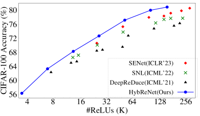
(a) ReLUs-Accuracy Pareto

(b) FLOPs saving

Figure 1: HybReNet outperforms state-of-the-art (SOTA) ReLU-optimization methods SENetsKundu et al. (2023a), SNLCho et al. (2022b), and DeepReDuceJha et al. (2021), achieving higher accuracy (CIFAR-100) and significant reduction in FLOPs while using fewer ReLUs.

Another major challenge that persists in this domain is identifying network attributes that enhance PI performance, as the effectiveness of PI-specific ReLU optimization techniques largely depends on the choice of input networks. This leads to significant performance disparities that cannot be solely ascribed to the FLOP count or accuracy of the input networks (refer to §3.2). Prior work Jha et al. (2021); Cho et al. (2022b); Kundu et al. (2023a) offer limited insight into their network selection. For instance, SENets Kundu et al. (2023a) and SNL Cho et al. (2022b) used WideResNet-22x8 for higher ReLU counts and ResNet18 for low ReLU counts. Thus, whether a network with specific features can consistently outperform across various ReLU counts or if targeted ReLU counts dictate the desired network attributes remains to be discovered.

The advancement in PI efficiency is further hindered by the limitations of the existing ReLU-optimization techniques. Coarse-grained ReLU optimizations Jha et al. (2021) encounter scalability issues, as their computational complexity varies linearly with the number of stages in a network. While fine-grained ReLU optimization Cho et al. (2022b); Kundu et al. (2023a) shows potential, its effectiveness is confined to specific ReLU distributions and tends to underperform in networks with higher ReLU counts or altered ReLU distribution (refer to §3.3).

Our techniques and insights. To this end, we thoroughly assess the design principles for ReLU and FLOPs efficiency and pose a fundamental question: Which essential insight needs to be integrated into the design framework for achieving FLOPs efficiency without compromising ReLU efficiency? Addressing this, we introduce a novel design principle, “ReLU-equalization,” which incorporates our key insight that by strategically expanding the network’s width and positioning ReLUs based on their criticality, we can regulate FLOPs in the deeper layers without sacrificing ReLU efficiency; thereby striking a dual balance.

Our in-depth investigation into key network attributes for PI efficiency yields a counterintuitive finding: wider networks enhance PI performance at higher ReLU counts, while the percentage of least-critical ReLUs in the network is crucial for PI efficacy at lower ReLU counts when ReLU pruning is employed. Prior work, unfortunately, does not leverage this insight, incurring substantial yet avoidable computational overheads. By leveraging this, we achieved a significant, up to 45$\times$, FLOP reduction when targeting lower ReLU counts.

Building on the above insights, we develop “DeepReShape,” a design framework to redesign the classical networks, with an efficient process of computational complexity $\mathcal{O}(1)$, and synthesize PI-efficient networks “HybReNet”. Our approach results in a substantial FLOP reduction with fewer ReLUs, outperforming the state-of-the-art in PI. Specifically, compared to SENet Kundu et al. (2023a), we achieve a 2.3$\times$ ReLU and 3.4$\times$ FLOP reduction at iso-accuracy, and a 2.1% accuracy gain with a 12.5$\times$ FLOP reduction at iso-ReLU on CIFAR-100. On TinyImageNet, our approach saves 12.4$\times$ FLOPs at iso-accuracy.

Contributions. Our key contributions are summarized as follows.

1. Perform an exhaustive characterization to identify the key network attributes for PI efficiency and demonstrate their applicability across a wide range of ReLU counts.

2. Propose a novel design principle ReLU-equalization, and designed a family of networks, HybReNet, tailored to PI constraints. Also, we devise ReLU-reuse, a channel-wise ReLU dropping technique to systematically reduce the ReLUs count by 16$\times$, allowing efficient ReLU optimization even at very low ReLU counts.

3. Rigorously evaluate our proposed techniques against SOTA in PI, SENets Kundu et al. (2023a), and SNLCho et al. (2022b); as well as SOTA FLOPs efficient models, ConvNeXt-V2 Woo et al. (2023) and RegNet Radosavovic et al. (2020), on CIFAR-100 and TinyImageNet datasets.

Scope of the paper. This paper delves into the challenges of strategically dropping ReLUs from the convolutional neural networks (CNNs) without resorting to any approximated computations for nonlinearity. Thus, we do not consider models that employ complex nonlinearities, such as transformer-based models and FLOPs efficient models like EfficientNet and MobileNetV3 , often relying on approximated nonlinear computations in PI. Also, we exclude the CrypTen-based PI in CNNs Tan et al. (2021); Peng et al. (2023), as it operates under different security assumptions and cost dynamics for linear and nonlinear computations .

2 Preliminary

Private inference protocols and threat model: We use Delphi Mishra et al. (2020) two-party protocols, as used in Jha et al. (2021); Cho et al. (2022b), for private inference. In particular, for linear layers, Delphi performs compute-heavy homomorphic operations Gentry et al. (2009); Fan & Vercauteren (2012); Brakerski et al. (2014); Cheon et al. (2017) in the offline phase (preprocessing) and additive secret sharing Shamir (1979) in the online phase, once the client’s input is available. Whereas, for nonlinear (ReLU) layers, it uses garbled circuits Yao (1986); Ball et al. (2019). Further, similar to Liu et al. (2017); Juvekar et al. (2018); Mishra et al. (2020); Rathee et al. (2020), we assume an honest-but-curious adversary where parties follow the protocols and learn nothing beyond their output shares.

Architectural building blocks: Figure 2 illustrates a schematic view of a standard four-stage network with design hyperparameters. Similar to ResNet He et al. (2016), it has a stem cell (to increase the channel count from 3 to $m$), followed by the network’s main body (composed of linear and nonlinear layers, performing most of the computation), followed by a head (a fully connected layer) yielding the scores for the output classes. The network’s main body is composed of a sequence of four stages, and the spatial dimensions of feature maps ($d_{k}\times d_{k}$) are progressively reduced by $2\times$ in each stage (except Stage1), and feature dimensions remain constant within a stage. We keep the structure of the stem cell and head fixed and change the structure of the network’s body using design hyperparameters.

Notations and definitions: Each stage is composed of identical blocks repeated $\phi_{1}$, $\phi_{2}$, $\phi_{3}$, and $\phi_{4}$ times in Stage1, Stage2, Stage3, and Stage4 (respectively), and known as stage compute ratios. The output channels in stem cell ($m$) are known as base channels, and the number of channels progressively increases by a factor of $\alpha$, $\beta$, and $\gamma$ in Stage2, Stage3, and Stage4 (respectively), and we termed it as stagewise channel multiplication factors. The spatial size of the kernel is denoted as $f\times f$ (e.g., $3\times 3$). These width and depth hyperparameters primarily determine the distribution of ReLUs, FLOPs, and (learnable) parameters in the network.

Channel scaling methods: When the network’s width is increased by uniformly scaling channels across all stages by the same factor, we refer to these networks as BaseCh, often used in networks optimized for FLOPs efficiency, where ($\alpha$, $\beta$, $\gamma$) values set to (2, 2, 2). For instance, WideResNets Zagoruyko & Komodakis (2016), or scaling the base channel from $m$=64 to $m$=128 in ResNets. Alternatively, networks widen by homogeneously augmenting the $\alpha$, $\beta$, and $\gamma$, are termed as StageCh. Such scaling is used for designing ReLU efficient baseline networks, for instance, CryptoNAS Ghodsi et al. (2020) and Sphynx Cho et al. (2022a). Lastly, when at least one of the values in ($\alpha$, $\beta$, $\gamma$) is different, we termed it as heterogeneous channel scaling, for instance, in semi-automated designed RegNets Radosavovic et al. (2020). Refer to Table 15 for details.

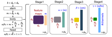
Figure 2: Depiction of architectural hyperparameters and feature dimensions in a four stage network. For ResNet18 $m$ = 64, $\phi_{1}$=$\phi_{2}$=$\phi_{3}$ =$\phi_{4}$=2, and $\alpha$=$\beta$=$\gamma$=2.

	Stage1	Stage2	Stage3	Stage4
$\frac{\#Params}{\#ReLU}$	$m(\frac{f^{2}}{d_{k}^{2}})$	$\alpha m(\frac{4f^{2}}{d_{k}^{2}})$	$\alpha\beta m(\frac{16f^{2}}{d_{k}^{2}})$	$\alpha\beta\gamma m(\frac{64f^{2}}{d_{k}^{2}})$
$\frac{\#FLOPs}{\#ReLU}$	$mf^{2}$	$\alpha mf^{2}$	$\alpha\beta mf^{2}$	$\alpha\beta\gamma mf^{2}$

Table 1: Network’s complexity (FLOPs and Params) per unit of nonlinearity varies with network’s width, and independent of the network’s depth. Consequently, Wider network need fewer ReLUs for a given complexity, compared to their deeper counterparts.

Criticality of ReLUs in a network: We employ the criticality metric $C_{k}$ from Jha et al. (2021) to quantify the significance of ReLUs’ within a network stage for overall accuracy. Higher $C_{k}$ values indicate more critical ReLUs, while the least significant ReLUs are assigned a value of zero (see Table 8 and 9).

Coarse-grained vs fine-grained ReLU optimization: The coarse-grained ReLU optimization method Jha et al. (2021) drops ReLUs at the level of an entire stage or a layer in the network. Whereas fine-grained ReLU optimizations (Cho et al., 2022b; Kundu et al., 2023a) target individual channels or activation. These approaches differ in performance, scalability, and configurability for achieving a specific ReLU count. The latter allows achieving any desired independent ReLU count automatically, while the former requires manual adjustments based on the network’s overall ReLU count and distribution. Nonetheless, the coarse-grained method demonstrates flexibility and adapting to various network configurations. In contrast, the fine-grained method exhibits less efficient adaptation and can lead to suboptimal performance.

3 Network Design and Optimization for Efficient Private Inference

We present our key observations highlighting the significance of network architecture and ReLUs’ distribution for end-to-end PI performance and motivate the need for redesigning the classical networks for efficient PI.

3.1 Addressing Pitfalls of Baseline Network Design for Efficient Private Inference

The conventional uniform channel scaling leads to suboptimal ReLU efficiency. Table 1 shows that the (stagewise) complexity of the network, quantified as #FLOPs and #Params Radosavovic et al. (2019), per units of ReLU nonlinearity scales linearly with base channel count $m$, while $\alpha$, $\beta$, and $\gamma$ introduce multiplicative effect. This implies that for a given network complexity, a network widened by augmenting $\alpha$, $\beta$, and $\gamma$ requires fewer ReLUs than the one widened by augmenting $m$. The uniform channel scaling in BaseCh networks, including WideResNet, often resorts to conservative ($\alpha$, $\beta$, $\gamma$) = (2, 2, 2), which limits the potential ReLU efficiency benefit from wider networks.

Homogeneous channel scaling offers superior ReLU efficiency until accuracy plateaus. In contrast to BaseCh networks, homogeneous channel scaling in StageCh networks significantly improves ReLU efficiency by removing the constraint on ($\alpha$, $\beta$, $\gamma$) (Figure 3(a)). Nonetheless, the superiority of StageCh networks remains evident until reaching accuracy saturation, which varies with network configuration. In particular, as shown in Figure 3(b), accuracy saturation for StageCh networks of ResNet18, ResNet20, ResNet32, and ResNet56 models begins at ($\alpha$, $\beta$, $\gamma$) = (4, 4, 4), (5, 5, 5), (5, 5, 5), and (6, 6, 6), respectively, suggesting deeper StageCh network plateau at higher ($\alpha$, $\beta$, $\gamma$) values. This observations challenge the assertion made in Ghodsi et al. (2020), that model capacity per ReLU peaks at ($\alpha$, $\beta$, $\gamma$) = (4, 4, 4). Thus, determining the accuracy saturation point a priori is challenging, raising an open question: To what extent can a network benefit from increased width for superior ReLU efficiency? Moreover, can employing ReLU optimization on StageCh networks effectively address accuracy saturation?

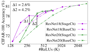
(a) ReLU efficiency: StageCh vs BaseCh

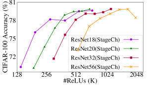
(b) Accuracy saturation in StageCh

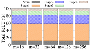
(c) ReLUs’ distribution: BaseCh networks

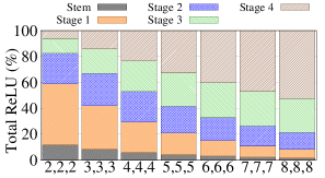
(d) ReLUs’ distribution: StageCh networks

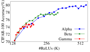
(e) Sensitivity analysis: ReLU efficiency

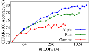
(f) Sensitivity analysis: FLOPs efficiency

Figure 3: (a) Homogeneous channel scaling in StageCh networks enables superior ReLU efficiency compared to uniform channel scaling in BaseCh networks; however, (b) the accuracy in StageCh networks tends to plateau unpredictably. (c,d) Unlike uniform channel scaling, homogeneous scaling reduces the proportion of least-critical ReLUs in StageCh networks. (e,f) Each network stage affects ReLU and FLOPs efficiency differently, requiring heterogeneous channel scaling for optimizing both ReLUs and FLOPs for efficient PI.

Homogeneous channel scaling alters the ReLUs’ distribution distinctively than uniform scaling. We investigate the effect of uniform and homogeneous channel scaling on the ReLU distribution of networks. Unlike uniform scaling, which scales all layer ReLUs uniformly, homogeneous scaling leads to a distinct ReLU distribution, with deeper layers exhibiting more significant changes. As depicted in Figure 3 (c,d), there is a noticeable decrease in the proportion of Stage1 ReLUs, while Stage4 witnesses a significant increase. Given the ReLUs’ criticality analysis in Table 8, this implies that the proportion of least-critical ReLUs is decreasing while the distribution of ReLUs among the other stages does not strictly adhere to their criticality order. This leads us to the following observation:

Observation 1: Homogeneous channel scaling reduces the percentage of least-critical ReLUs in the network.

Heterogeneous channel scaling is required for optimizing ReLU and FLOPs efficiency simultaneously. To answer the question of potential benefits from wider networks, we perform a sensitivity analysis and evaluate the influence of each stagewise channel multiplication factor on the network’s ReLU and FLOPs efficiency. We systematically vary one factor at a time, starting from 2, while other factors are held constant at 2, in ResNet18 with $m$=16. We observe that augmenting $\alpha$ and $\beta$ values improves ReLU efficiency; notably, the latter optimizes the performance marginally better than the former until a saturation point is reached (see 3(c)). Whereas, FLOPs efficiency is most effectively improved by augmenting $\alpha$, outperforming $\beta$ enhancements while augmenting $\gamma$ values yields the worst FLOP efficiency (see 3(d)). This suggests that FLOPs in the deeper layers of StageCh networks can be regulated without impacting ReLU efficiency.

We note that the semi-automated designed networks RegNets Radosavovic et al. (2020) employ heterogeneous channel scaling. However, they confine $1.5\leq$($\alpha$, $\beta$, $\gamma$) $\leq 3$ to optimize FLOPs efficiency, which in turn limits their ReLU efficiency (see Figure 11(c)). Thus, despite a line of seminal work on the network’s width expansion Zagoruyko & Komodakis (2016); Radosavovic et al. (2019); Lee et al. (2019); Dollár et al. (2021), the approaches to leverage the potential benefits of increased width for simultaneously optimizing ReLUs and FLOPs efficiency remains an open challenge. The above analyses lead us to the following observation:

Observation 2: Each network stage heterogeneously impacts both ReLU and FLOPs efficiency, a nuanced aspect largely overlooked by prior channel scaling methods, rendering them inadequate for the simultaneous optimizing ReLUs and FLOPs counts for efficient private inference.

Strategically scaling channels by arranging ReLUs in their criticality order can regulate the FLOPs in deeper layers without compromising ReLU efficiency. Following from the observations 1 and 2, we propose to scale the channels until all ReLUs are aligned in the criticality order. Thus, Stage3 dominates the distribution as it has the most critical ReLUs, followed by Stage2, Stage4, and Stage1 (Table 8). Unlike StageCh networks, widening beyond the point where the ReLUs are aligned in their criticality order does not alter their relative distribution (Figure 4(a)). This leads to higher $\alpha$ and $\beta$ values, which boost ReLU efficiency, with restrictive $\gamma$ ($\gamma<$4) regulating FLOPs in deeper layers, promoting FLOP efficiency.

Consequently, our approach of heterogeneous channel scaling achieves ReLU efficiency on par with StageCh networks with fewer FLOPs. Figure 4(b,c) demonstrates that the ReLUs’ criticality-aware ResNet18 network 5x5x3x maintains similar ReLU efficiency with a 2$\times$ reduction in FLOPs compared to the StageCh network 5x5x5x. This FLOP reduction is consistently attained across the entire spectrum of ReLU counts, employing both fine-grained and coarse-grained ReLU optimization. These results lead to the following observation:

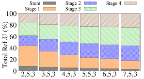
(a) HRN-5x5x3x (Proposed)

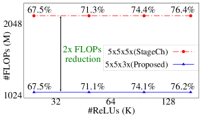
(b) FLOPs saving w/ SNL

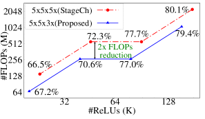
(c) FLOPs saving w/ DeepReDuce

Figure 4: (a) Unlike StageCh networks, once the network’s ReLUs are aligned in their criticality order, here at point ($\alpha$, $\beta$, $\gamma$)=(5, 5, 3), increasing $\alpha$ does not alter their relative distribution. (b,c) ReLUs’ criticality-aware network widening method saves 2$\times$ FLOPs by regulating the FLOPs in deeper layers while maintaining ReLU efficiency over a wide range of ReLU counts.

Observation 3: ReLUs’ criticality-aware network widening method optimizes FLOPs efficiency without sacrificing the ReLU efficiency, which meets the demands of efficient PI.

3.2 Addressing Fallacies in Network Selection for ReLU Optimization

Selecting the appropriate input network for ReLU optimization methods is far from intuitive. Table 2 lists input networks used in previous ReLU optimization methods with their relevant characteristics, while Figure 5 demonstrates how different input networks affect the performance of coarse (DeepReDuce) and fine-grained (SNL) ReLU optimization methods. For the former, accuracy differences of 12.9% and 11.6% are observed at higher and lower iso-ReLU counts. These differences cannot be ascribed to the FLOPs or accuracy of the baseline network alone. For instance, ResNet18 outperforms WideResNet22x8 despite having 4.4$\times$ fewer FLOPs and a lower baseline accuracy, and ResNet32 outperforms VGG16 even though the latter has 4.76$\times$ more FLOPs and a higher baseline accuracy.

Likewise, fine-grained ReLU optimization (SNL) exhibits significant accuracy differences when employed on ResNets and WideResNets, especially at lower ReLU counts, as shown in Figure 5(b). While WideResNet models outperform beyond 200K ReLUs, there are 3.2% and 4.6% accuracy gaps at 25K and 15K ReLUs between ResNet18 and WideResNet16x8. The above empirical observation led to the following observation:

Observation 4: Performance of ReLU optimization methods, whether coarse or fine-grained, strongly correlates with the choice of input networks, leading to substantial performance disparities.

ReLU optimization method	Input networks
Delphi (Mishra et al., 2020)	ResNet32
SAFENets (Lou et al., 2021)	ResNet32, VGG16
DeepReDuce (Jha et al., 2021)	ResNet18
SNL (Cho et al., 2022b)	ResNet18, WRN22x8
SENet (Kundu et al., 2023a)	ResNet18, WRN22x8

	ResNet32	ResNet18	WRN22x8	VGG16
FLOPs	70M	559M	2461M	333M
ReLUs	303K	557K	1393K	285K
Acc	71.67%	79.06%	81.27%	75.08%

Table 2: Baseline networks used for advancing ReLU-Accuracy Pareto (CIFAR-100) in prior PI-specific ReLU optimization methods.

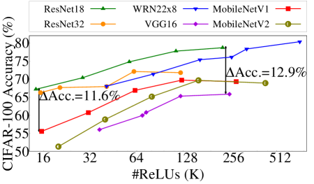
(a) DeepReDuce at iso-ReLU

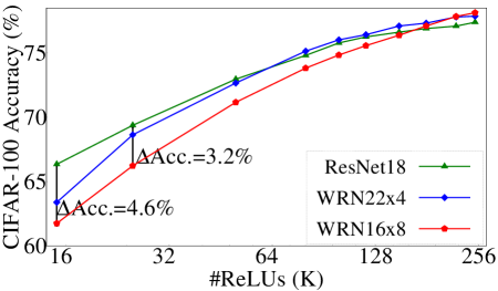
(b) SNL at iso-ReLU

Figure 5: ReLU optimization, whether coarse or fine-grained, performance exhibits significant disparities based on the input networks.

Key network attributes for PI efficiency vary across targeted ReLU counts. To identify the key network attributes for PI efficiency across a wide range of ReLU counts, we examine three ResNet18 variants with identical ReLU counts but different ReLUs’ distribution and FLOPs counts (Table 3). These are realized by channel reallocation, and the configurations 2x2x2x($m$=32), 4x4x4x($m$=16), and 3x7x2x($m$=16) correspond to stagewise channel counts as [32,64,128,256], [16, 64, 256, 1024], and [16, 48, 336, 672] respectively. We analyze their performance using the DeepReDuce and SNL ReLU optimization, as shown in Figure 6.

A consistent trend emerges from both ReLU optimization methods: Wider models 4x4x4x($m$=16) and 3x7x2x($m$=16) outperform 2x2x2x($m$=32) at higher ReLU counts; however, even with $\approx 4\times$ fewer FLOPs, 2x2x2x($m$=32) excel at lower ReLU counts. This superior performance stems from the higher percentage (58.82%) of least-critical (Stage1) ReLUs in 2x2x2x($m$=32). When targeting low ReLU counts, ReLU optimization methods primarily drop ReLUs from Stage1 Jha et al. (2021); Cho et al. (2022b); Kundu et al. (2023a). Thus, networks with a higher percentage of Stage1 ReLUs preserve more ReLUs from critical stages, mitigating accuracy degradation. Furthermore, this emphasizes the importance of strategically allocating channels, even when aiming for higher ReLU counts: 3x7x2x($m$=16) matches the ReLU efficiency of 4x4x4x($m$=16) with 30% fewer FLOPs by allocating more channels to Stage3 and fewer to Stage4.

Model	Acc(%)	FLOPs	ReLUs	Stagewise ReLUs’ distribution
				Stage1	Stage2	Stage3	Stage4
2x2x2x(m=32)	75.60	141M	279K	58.82%	23.53%	11.76%	5.88%
4x4x4x(m=16)	78.16	661M	279K	29.41%	23.53%	23.53%	23.53%
3x7x2x(m=16)	78.02	466M	260K	31.50%	18.90%	33.07%	16.54%

Table 3: A case study to investigate the Capacity-Criticality-Tradeoff: Three Iso-ReLU ResNet18 networks with different ReLUs’ distribution and FLOPs count, achieved by reallocating channels per stage. The baseline accuracy is for CIFAR-100 dataset.

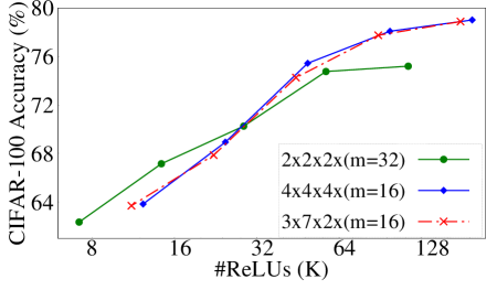
(a) DeepReDuce at iso-ReLU

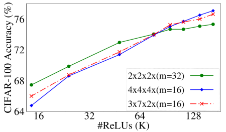
(b) SNL at iso-ReLU

Figure 6: Capacity-Criticality-Tradeoff results: Figures (a) and (b) show the ReLU-Accuracy tradeoff for networks in Table 3 using DeepReDuce and SNL.

The above findings offer insight into the network selection for prior ReLU optimization methods. Specifically, the choice of WRN22x8 (with 48.2% Stage1 ReLUs) for higher ReLU counts while ResNet18 for lower ReLU counts in fine-grained ReLU optimization Cho et al. (2022b); Kundu et al. (2023a). Moreover, it also explains the accuracy trends depicted in Figure 5(b), the higher the Stage1 ReLU proportion (58.8% for ResNet18, 47.7% for WRN22x4, and 43.9% for WRN16x8), the higher the accuracy at lower ReLU counts.

Interestingly, we note that the above networks with a higher percentage of least-critical (Stage1) ReLUs inherently have fewer overall ReLUs (e.g., 1392.6K for WRN22x8 and 557K ResNet18). This might suggest that these networks utilize their ReLUs more effectively, especially when there are fewer ReLUs, leading them to excel at lower ReLU counts. However, a counter-example in Appendix C.3 reaffirms our conclusion for the key factor driving PI performance at lower ReLU counts. These analyses lead to the following observation:

Observation 5: Wider networks are superior only at higher ReLU counts, while networks with higher percentage of least-critical ReLUs outperform at lower ReLU counts (Capacity-Criticality-Tradeoff).

3.3 Mitigating the Limitations of Fine-grained ReLU Optimization

Fine-grained ReLU optimization is not always the best choice. While fine-grained ReLU optimization has demonstrated its effectiveness in classical networks such as ResNet18 and WideResNet — especially when Stage1 dominates the network’s ReLU distribution Cho et al. (2022b); Kundu et al. (2023a) — its advantages are not universal. To better understand its range of efficacy, we compared it against DeepReDuce on PI-amenable wider models: 4x4x4x($m$=16) and 3x7x2x($m$=16) (Table 3).

As shown in Figure 7(a) and 7(b), DeepReDuce outperforms SNL by a significant margin (up to 3%-4%). This suggests that the benefits of fine-grained ReLU optimization are highly dependent on specific ReLU distributions, and it reduces when Stage1 does not dominate the network’s ReLU distribution. This trend is also observed in ReLU criticality-aware networks, where Stage3 dominates the distribution of ReLUs (see Figure 19). This empirical evidence collectively suggests that fine-grained ReLU optimization might limit the benefits of increased network complexity introduced through stagewise channel multiplication enhancements. Nonetheless, the performance gap is less pronounced when the network’s overall ReLU count is reduced by half by using ReLU-Thinning Jha et al. (2021), which drops the ReLUs from alternate layers.

	C100	Baseline	220K	180K	150K	120K	100K	80K	50K
ResNet18 (557.06K)	Vanilla	78.68	77.09	76.9	76.62	76.25	75.78	74.81	72.96
	w/ Th.	76.95	77.03	76.92	76.54	76.59	75.85	75.72	74.44
	$\Delta$	-1.73	-0.06	0.02	-0.08	0.34	0.07	0.91	1.48
ResNet34 (966.66K)	Vanilla	79.67	76.55	76.35	76.26	75.47	74.55	74.17	72.07
	w/ Th.	79.03	77.94	77.65	77.67	77.32	76.69	76.32	74.50
	$\Delta$	-0.64	1.39	1.30	1.41	1.85	2.14	2.15	2.43
WRN22x8 (1392.64K)	Vanilla	80.58	77.58	76.83	76.15	74.98	74.38	73.16	71.13
	w/ Th.	79.59	78.91	78.6	78.41	78.05	77.22	75.94	72.74
	$\Delta$	-0.99	1.33	1.77	2.26	3.07	2.84	2.78	1.61

Table 4: A significant accuracy boost (on CIFAR-100) is achieved when ReLU-Thinning is employed prior to SNL, despite the less accurate ReLU-Thinned models. $\Delta$ = Acc(w/ Th.)-Acc(Vanilla).

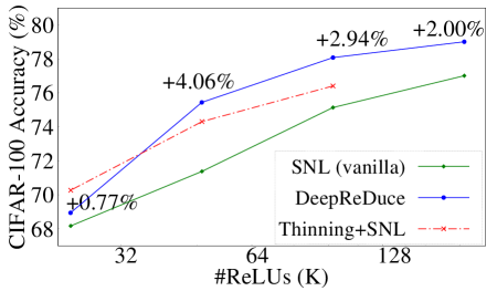
(a) 4x4x4x($m$=16)

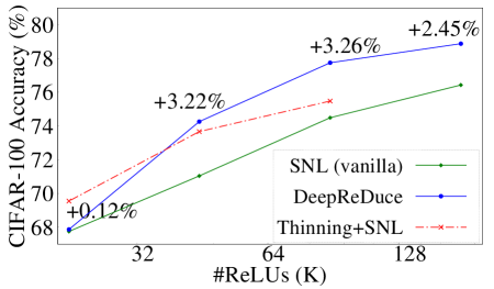
(b) 3x7x2x($m$=16)

Figure 7: DeepReDuce outperforms SNL by a significant margin (up to 4%) when altering network’s ReLUs distribution; however, using SNL on ReLU-Thinned networks reduces the accuracy gap.

Narrowing the search space improves the performance of fine-grained ReLU optimization. To further examine the efficacy of ReLU-Thinning for classical networks, we adopt a hybrid ReLU optimization approach, and ReLU-Thinning is employed before SNL optimization. Surprisingly, even when baseline Thinned models are less accurate, a significant accuracy boost (up to 3% at iso-ReLUs) is observed, which is more pronounced for networks with higher #ReLUs (ResNet34 and WRN22x8, in Table 4). Since ReLU-Thinning drops the ReLUs from the alternate layers, irrespective of their criticality, its integration into existing ReLU optimization methodologies would not impact their overall computational complexity and remains effective for reducing the search space to identify critical ReLUs. This leads us to the following observation:

Observation 6: While altering the network’s ReLU distribution can lead to suboptimal performance in fine-grained ReLU optimization, ReLU-Thinning emerges as an effective solution to bridge the performance gap, also beneficial for classical networks with higher overall ReLU counts.

4 DeepReShape

Drawing inspiration from the above observations and insights, we propose a novel design principle termed ReLU equalization (Figure 8) and re-design classical networks. This led to the development of a family of models HybReNet, tailored to the needs of efficient PI (Table 16). Additionally, we propose ReLU-reuse, a (structured) channel-wise ReLU dropping method, enabling efficient PI at very low ReLU counts.

4.1 ReLU Equalization and Formation of HybReNet

Given a baseline input network, where ReLUs are not necessarily aligned in their criticality order, ReLU equalization redistributes the network’s ReLUs in their criticality order, meaning the (most) least critical stage has a (highest) lowest fraction of the network’s total ReLU count (Figure 8). Equalization is achieved by an iterative process, as outlined in Algorithm 1. In each iteration, the relative distribution of ReLUs in two stages is aligned in their criticality order by adjusting either their depth or width or both hyperparameters.

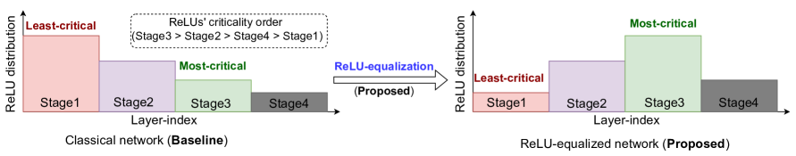
Figure 8: Illustration of ReLU-equalization: Unlike classical networks (e.g., ResNet), where ReLUs’ are not positioned is their criticality order, ReLU-equalization aligns network’s ReLUs in their criticality order.

Algorithm 1 ReLU equalization

Input: Network $Net$ with stages $S_{1}$,…,$S_{D}$; $C$ a sorted list of most to least critical stage; stage-compute ratio $\phi_{1}$,…,$\phi_{D}$; and stagewise channel multiplication factors $\lambda_{1}$,…, $\lambda_{(D-1)}$.
Output: ReLU-equalized versions of network $Net$.

1:for $i$ = 1 to $D$-1 do

2:     $S_{k}$ = $C[i]$ $\triangleright$ $C[1]$ is most critical stage

3:     $S_{t}$ = $C[i+1]$ $\triangleright$ $C[2]$ is second-most critical stage

4:     while #ReLUs($S_{k}$) $>$ #ReLUs($S_{t}$) do $\triangleright$ ReLUs in two stages are aligned in their criticality order

5:         $\frac{\phi_{k}\times\big{(}\prod_{j=1}^{k-1}\lambda_{j}\big{)}}{2^{k-1}}$ $>$ $\frac{\phi_{t}\times\big{(}\prod_{j=1}^{t-1}\lambda_{j}\big{)}}{2^{t-1}}$ $\triangleright$ Rearranging ReLUs by adjusting width and depth parameters

6:     end while

7:end for

8:return A set of $\phi_{1}$,…,$\phi_{D}$ and $\lambda_{1}$,…,$\lambda_{(D-1)}$ that satisfies the compound inequality: #ReLUs($C[1]$) $>$ #ReLUs($C[2]$) $>$ … $>$ #ReLUs($C[D-1]$) $>$ #ReLUs($C[D]$)

Specifically, for a network of $D$ stages and a predetermined criticality order, given compute ratios $\phi_{1}$, $\phi_{2}$, …, $\phi_{D}$ and stagewise channel multiplication factors $\lambda_{1}$, $\lambda_{2}$, …, $\lambda_{(D-1)}$, the ReLU equalization algorithm outputs a compound inequality after $D$-1 iterations. We now employ Algorithm 1 on a standard four-stage ResNet18 model with the given criticality order as (from highest to lowest): Stage3 $>$ Stage2 $>$ Stage4 $>$ Stage1 (refer to Table 8). During the equalization process, only the model’s width hyper-parameters are adjusted, as wider models tend to be more ReLU efficient. Consequently, the algorithm yields the following expression:

$$\#ReLUs(S_{3})>\#ReLUs(S_{2})>\#ReLUs(S_{4})>\#ReLUs(S_{1})$$

$$\implies\phi_{3}\Big{(}\frac{\alpha\beta}{16}\Big{)}>\phi_{2}\Big{(}\frac{\alpha}{4}\Big{)}>\phi_{4}\Big{(}\frac{\alpha\beta\gamma}{64}\Big{)}>\phi_{1}$$

$$\text{ReLU equalization through width}\;(\phi_{1}=\phi_{2}=\phi_{3}=\phi_{4}=2,\;\text{and}\;\alpha\geq 2,\beta\geq 2,\gamma\geq 2):$$

$$\implies\frac{\alpha\beta}{16}>\frac{\alpha}{4}>\frac{\alpha\beta\gamma}{64}>1\implies\alpha\beta>16,\;\alpha>4,\;\alpha\beta\gamma>64,\;\beta>4,\;\beta\gamma<16,\;\text{and}\;\gamma<4$$

$$\text{Solving the above compound inequalities provides the following}\;(\beta,\gamma)\;\text{pairs and the range of}\;\alpha:$$

$$\text{The}\;(\beta,\gamma)\;\text{pairs are:}\;(5,2)\;\&\;\alpha\geq 7;\;(5,3)\;\&\;\alpha\geq 5;\;(6,2)\;\&\;\alpha\geq 6;\;(7,2)\;\&\;\alpha\geq 5$$

We obtain four pairs of ($\beta$, $\gamma$), each having a range of $\alpha$ value. We choose the smallest $\alpha$ needed for ReLU equalization, as increasing $\alpha$ beyond this point does not improve the performance when ReLU optimization is used; also, the relative distribution of ReLUs remains stable (see Appendix A). Thus, we achieve four baseline HybReNets: HRN-5x5x3x, HRN-5x7x2x, HRN-6x6x2x, and HRN-7x5x2x. The architectural details of these four HRNs are presented in Table 16.

4.2 ReLU-reuse

We further refine the baseline network’s architecture to increase ReLU nonlinearity utilization by introducing ReLU-reuse, which selectively applies ReLUs to a contiguous subset of channels while the remaining channels reuse them. This approach differs from previous channel-wise ReLU optimizations, where channels are either uniformly scaled down throughout the network Jha et al. (2021) or only a subset of channels utilize ReLUs without reusing them Cho et al. (2022b). Our ReLU-reuse mechanism allows for efficient PI at extremely low ReLU counts (e.g., 3.2K ReLUs on CIFAR-100 dataset).

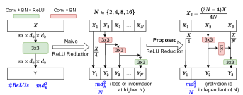
Figure 9: Proposed ReLU-reuse where ReLUs are selectively reused across channels, reducing #ReLUs up to 16$\times$.

Specifically, feature maps of the layer are divided into $N$ groups, and ReLUs are employed only in the last group (Figure 9). However, increasing the value of $N$ results in a significant accuracy loss despite $1\times 1$ convolution being employed for cross-channel interaction. This is likely due to the loss of cross-channel information arising from more divisions in the feature maps (see our ablation study in Table 14). To address this issue, we devise a mechanism that decouples the number of divisions in feature maps from the ReLU reduction factor $N$. Precisely, one-fourth of channels are utilized for feature reuse, while a $Nth$ fraction of feature maps are activated using ReLUs, and the remaining feature maps are processed solely with convolution operations, resulting in only three groups. It is important to note that using the ReLUs in the last group of feature maps increases the effective receptive field as these neurons can consider a larger subset of feature maps using the skip connections Gao et al. (2019).

4.3 Putting it All Together

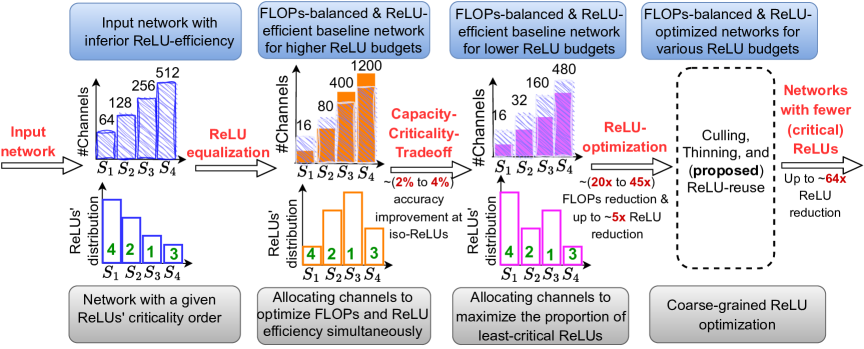
Figure 10: The DeepReShape network redesigning pipeline. ReLU’s criticality-aware strategic allocation of channels (gray boxes) outputs FLOPs-balanced ReLU-efficient baseline networks for various ReLU counts (blue boxes). Numbers in green denote criticality order (Stage3 is most critical).

We developed the DeepReShape framework to re-design the classical networks for efficiency PI across a wide range of ReLU counts. Figure 10. Given an input network with a specific ReLUs’ criticality order, the ReLU-equalization step aligns the network’s ReLU in their criticality order by adjusting width hyper-parameters. This step allows for maximizing ReLU efficiency without incurring superfluous FLOPs by allocating fewer channels in the initial stages and increasing them in the deeper stages. In the second step, following the Criticality-Capacity-Tradeoff, the width is adjusted such that Stage1 dominates the ReLUs’ distribution. This is achieved by a straightforward step: setting $\alpha$=2 in the ReLU-equalized networks since decreasing $\alpha$ results in an increased percentage of Stage1 ReLUs, and distribution of ReLUs in all but Stage1 follow their criticality order (see Table 9). This step allows for a substantial FLOP reduction, up to 45$\times$, by allocating fewer channels in all the stages. We call the networks resulting from step1 and step2 as HybReNets (HRNs). The baseline HRNs from step2 are: HRN-2x5x3x, HRN-2x7x2x, HRN-2x6x2x, and HRN-2x5x2x (Table 17).

ReLU-optimization steps for HybReNets: We choose to employ coarse-grained ReLU optimization steps in HRNs, as they outperform fine-grained ReLU optimization when the ReLU distribution undergoes changes in traditional networks, as shown in Figure 7 and Appendix C.4. In particular, we eliminate all the ReLUs from Stage1 (ReLU Culling) if it dominates the network’s overall ReLU distribution, e.g., HRNs with $\alpha$=2. For subsequent stages, we utilize ReLU-Thinning, which removes ReLUs from alternate layers without considering their criticality. We further reduce the ReLU count by implementing ReLU-reuse with an appropriate reduction factor (see Algorithm 2).

Complexity analysis of HybReNet design: For a $D$ stage network with a predefined criticality order for stagewise ReLUs, the process of ReLU equalization typically involves considering 2$D$-1 hyperparameters, including $D$ stage compute ratios and $D$-1 stagewise channel multiplication factors. However, for HRNs, this hyperparameter count is reduced to $D$-1 since ReLU equalization is achieved solely by modifying the network’s width. Contrasting with SOTA network designing methods Radosavovic et al. (2020); Liu et al. (2022), which build networks from scratch, the hyperparameters involved in ReLU equalization are determined by solving a compound inequality and do not require additional network training. Consequently, the complexity of designing HRNs can be characterized as $\mathcal{O}(1)$. A detailed discussion is included in Appendix E.5.

Note that employing coarse-grained ReLU optimization does not exacerbate the complexity of HRNs. This is attributed to the alignment of ReLUs within HRNs based on their criticality order, which necessitates only a single iteration (see Algorithm 2). In contrast, when ReLUs in the input network are organized without regard to their criticality order (e.g., classical networks such as ResNets and WideResNets), a single iteration produces suboptimal results, requiring $D$-1 iterations Jha et al. (2021). Thus, the complexity of ReLU optimization for HRNs is reduced to $\mathcal{O}(1)$ from $\mathcal{O}(D)$.

5 Experimental Results

Analysis of HybReNets Pareto points: Figure 1 shows that HybReNet advances the ReLU-accuracy Pareto with a substantial reduction in FLOPs – a factor overlooked in prior PI-specific network optimization. We present a detailed analysis of network configurations and ReLU optimization steps and quantify their benefits for ReLUs and FLOP reduction. We use ResNet18-based HRN-5x5x3x for ReLU-accuracy comparison with SOTA PI methods in Figure 1, as its FLOPs efficiency is superior to other HRNs (Table 16).

Table 5: Network configurations and ReLU optimization steps used for the Pareto points in Figure 1. Accuracies (CIFAR-100) are separately shown for vanilla KD Hinton et al. (2015) and DKD Zhao et al. (2022), highlighting the benefits of improved architectural design and distillation method.(Re2 denotes ReLU-reuse)

HybReNet	$m$	ReLU optimization steps			#ReLU	#FLOPs	Accuracy(%)		Acc./ReLU
		Culled	Thinned	Re2			KD	DKD
5x5x3x	16	NA	S1+S2+S3+S4	NA	163.3K	1055.4M	79.34	80.86	0.50
2x5x3x	32	S1	S2+S3+S4	NA	104.4K	714.1M	77.63	79.96	0.77
2x5x3x	16	S1	S2+S3+S4	NA	52.2K	178.5M	74.98	77.14	1.48
2x5x3x	8	S1	S2+S3+S4	NA	26.1K	44.6M	70.36	72.65	2.78
2x5x3x	16	S1	S2+S3+S4	4	13.1K	121.6M	67.30	68.25	5.23
2x5x3x	16	S1	S2+S3+S4	8	6.5K	130.5M	62.68	63.29	9.70
2x5x3x	16	S1	S2+S3+S4	16	3.2K	137.2M	56.24	56.33	17.26

The key takeaway from Table 5 is that tailoring the network features for PI constraint significantly reduces FLOPs and ReLUs. Specifically, lowering $\alpha$ value and base channel count led to 23.6$\times$ fewer FLOPs in HRN-2x5x3x($m$=8), compared to HRN-5x5x3x($m$=16). Furthermore, we notice a significant accuracy boost by employing a simple yet efficient logit-based distillation method DKD Zhao et al. (2022), as the ReLU-reduced models greatly benefit from decoupling the target and non-target class distillation.

HybReNets outperform state-of-the-art in private inference: Table 6 presents competing design points for SENet Kundu et al. (2023a) and SNL Cho et al. (2022b), and we select HybReNet points (see Table 5 and Table 11 for configuration and optimization details) offering both accuracy and latency benefits for a fair comparison. The runtime breakdown is presented as homomorphic (HE) latency Brakerski et al. (2014), arises from linear operations (convolution and fully-connected layers), and Garbled-circuit (GC) latency Ball et al. (2019), resulting from nonlinear (ReLU) operations. See the experiential setup details in Appendix H.

Table 6: Comparison of HybReNet with state-of-the-art in private inference: SENet Kundu et al. (2023a) and SNL Cho et al. (2022b). HybReNet exhibits superior ReLU and FLOPs efficiency and achieve a substantial reduction in latency. #Re and #FL denote ReLU and FLOPs counts; Acc. is top-1 accuracy; Lat. is the runtime for one private inference, including Homomorphic (HE) and Garbled-circuit(GC) latencies.

		SOTA in Private Inference						HybReNet(Ours)						Improvements
		#Re	#FL	Acc.	HE	GC	Lat.	#Re	#FL	Acc.	HE	GC	Lat.	#Re	#FL	Acc.	HE	GC	Lat.
CIFAR-100	SENets	300	2461	80.54	1004	33.7	1037	163	1055	80.86	770	18.4	788	1.8$\times$	2.3$\times$	0.3	1.3$\times$	1.8$\times$	1.3$\times$
		240	2461	79.81	1004	27.0	1031	163	1055	80.86	770	18.4	788	1.5$\times$	2.3$\times$	1.1	1.3$\times$	1.5$\times$	1.3$\times$
		180	2461	79.12	1004	20.2	1024	163	1055	80.86	770	18.4	788	1.1$\times$	2.3$\times$	1.7	1.3$\times$	1.1$\times$	1.3 $\times$
		50	559	75.28	268	5.6	274	52	179	77.14	123	5.9	129	1.0$\times$	3.1$\times$	1.9	2.2$\times$	0.9$\times$	2.1$\times$
		25	559	70.59	268	2.8	271	26	45	72.65	49	2.9	52	0.9$\times$	12.5$\times$	2.1	5.5$\times$	1.0$\times$	5.2$\times$
	SNL	15	559	67.17	268	1.7	270	13	179	68.25	123	1.5	124	1.1$\times$	3.1$\times$	1.1	2.2$\times$	1.1$\times$	2.2$\times$
		13	559	66.53	268	1.5	270	13	179	68.25	123	1.5	124	1.0$\times$	3.1$\times$	1.7	2.2$\times$	1.0$\times$	2.2$\times$
TinyImageNet	SENets	300	2227	64.96	927	33.7	961	327	1055	64.92	526	36.7	563	0.9$\times$	2.1$\times$	0.0	1.8$\times$	0.9$\times$	1.7$\times$
		142	2227	58.90	927	16.0	943	104	179	58.90	97	11.7	108	1.4$\times$	12.4$\times$	0.0	9.6$\times$	1.4$\times$	8.7$\times$
	SNL	489	9830	64.42	3690	55.0	3745	653	4216	67.58	2029	73.4	2102	0.7$\times$	2.3$\times$	3.2	1.8$\times$	0.7$\times$	1.8$\times$
		489	9830	64.42	3690	55.0	3745	418	2842	66.10	1307	45.0	1352	1.2$\times$	3.5$\times$	1.7	2.8$\times$	1.2$\times$	2.8$\times$
		298	2227	64.04	927	33.5	961	327	1055	64.92	526	36.7	563	0.9$\times$	2.1$\times$	0.9	1.8 $\times$	0.9$\times$	1.7$\times$
		100	2227	58.94	927	11.2	939	104	179	58.90	97	11.7	108	1.0$\times$	12.4$\times$	0.0	9.6$\times$	1.0$\times$	8.7$\times$
		59	2227	54.40	927	6.6	934	52	712	54.46	329	5.9	335	1.1$\times$	3.1$\times$	0.1	2.8$\times$	1.1$\times$	2.8$\times$

On CIFAR-100, SENet requires 300K ReLUs and 2461M FLOPs to reach 80.54% accuracy, whereas HRN-5x5x3x achieves 80.86% accuracy with only 163K ReLUs and 1055M FLOPs, providing 1.8$\times$ ReLU and 2.3$\times$ FLOPs saving. Similarly, at 25K ReLUs, our approach achieves a 2.1% accuracy gain with 12.5$\times$ FLOP reduction, thereby saving 5.2$\times$ runtime. Even at an extremely low ReLU count of 13K, HRN is 1.7% more accurate and achieves 2.2$\times$ runtime saving, compared to the SNL.

On TinyImageNet, HybReNets outperform SENet at both 300K and 142K ReLUs, improving runtime by 1.7$\times$ and 8.7$\times$, respectively. Compared to SNL at 489K ReLUs, HybReNets are 3.2% (1.7%) more accurate with a 1.8$\times$ (2.8$\times$) reduction in runtime. At lower ReLU counts of 100K and 59K, HybReNets match the accuracy with SNL and achieve a 12.4$\times$ and 3.1$\times$ FLOP reduction, which results in 8.7$\times$ and 2.8$\times$ runtime improvement, respectively.

Our primary insight from Table 6 is that FLOP reduction does not inherently guarantee a proportional reduction in HE latency, whereas a direct correlation exists between ReLU reduction and GC latency savings. In particular, a $\sim$12.5$\times$ FLOP reduction translates to 5.2$\times$ and 8.7$\times$ latency reduction on CIFAR-100 and TinyImageNet, respectively. This is due to the fact HE latency has an intricate dependency on the input/output packing Aharoni et al. (2023), rotational complexity Lou et al. (2020b; a); Huang et al. (2022) and slot utilization Lee et al. (2022). We refer the readers to Juvekar et al. (2018) for details.

Generality case study on ResNet34: We select ResNet34 for the DeepReShape generality study for two key reasons: (1) its consistent use for the case study in prior PI-specific network optimization studies Jha et al. (2021); Cho et al. (2022b); Kundu et al. (2023a), and (2) its stage compute ratio ($\phi_{1}$=3, $\phi_{2}$=4, $\phi_{3}$=6, and $\phi_{4}$=3) distinguishes it from ResNet18, results in different sets of HRN networks, HRN-4x6x3x and HRN-4x9x2x, upon applying Algorithm 1. We use HRN-4x6x3x for comparison with SOTA in Table 7. Network configuration and ReLU optimization details are presented in Table 12.

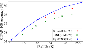
(a) ResNet34 on CIFAR-100

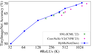
(b) ResNet34 on TinyImageNet

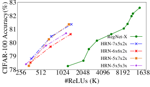
(c) HRN vs RegNet on CIFAR-100

Figure 11: HybReNets outperform SOTA ReLU-optimization methods applied to ResNet34 and also surpass SOTA FLOPs efficient models: RegNetsRadosavovic et al. (2020) and ConvNeXt-V2 Woo et al. (2023).

HybReNet advances the ReLU-accuracy Pareto on both CIFAR-100 and TinyImageNet, shown in Figures 11 (a, b). Table 7 quantifies the FLOPs-ReLU-Accuracy benefits and runtime savings. On CIFAR-100, compared to SOTA, HybReNet improves runtime by 3.1$\times$ with a significant gain in accuracy — 9.8%, 7.2%, 5.9%, and 2.1% at 15K, 25K, 30K and 50K ReLUs (respectively). Further on TinyImageNet, SNL requires 300K ReLUs and 4646M FLOPs to reach 64% accuracy, whereas HybReNet matches this accuracy with 8.8$\times$ fewer FLOPs, leading to a runtime improvement of 6.3$\times$. Conclusively, it highlights the effectiveness of DeepReShape and validates its generality for different network configurations and datasets.

Table 7: ResNet34-based HybReNets outperform SOTA PI methods Kundu et al. (2023a); Cho et al. (2022b) employed on ResNet34, and also surpass the SOTA FLOPs efficient models ConvNeXt-V2Woo et al. (2023) . #Re and #FL denote ReLU and FLOPs counts; Acc. is top-1 accuracy; Lat. is the runtime for one PI.

		SOTA in Private Inference (on ResNet34)						HybReNet(Ours)						Improvements
		#Re	#FL	Acc.	HE	GC	Lat.	#Re	#FL	Acc.	HE	GC	Lat.	#Re	#FL	Acc.	HE	GC	Lat.
CIFAR-100	SENet	200	1162	78.80	459	22.5	482	134	527	79.56	404	15.1	419	1.5$\times$	2.2 $\times$	0.8	1.1$\times$	1.5$\times$	1.1$\times$
		80	1162	76.66	459	9.0	468	67	132	76.91	140	7.5	148	1.2$\times$	8.8$\times$	0.3	3.3$\times$	1.2$\times$	3.2$\times$
		50	1162	74.84	459	5.6	465	67	132	76.91	140	7.5	148	0.7$\times$	8.8$\times$	2.1	3.3$\times$	0.7$\times$	3.1$\times$
	SNL	30	1162	71.00	459	3.4	462	67	132	76.91	140	7.5	148	0.4$\times$	8.8$\times$	5.9	3.3$\times$	0.4$\times$	3.1$\times$
		25	1162	69.68	459	2.8	462	67	132	76.91	140	7.5	148	0.4$\times$	8.8$\times$	7.2	3.3$\times$	0.4$\times$	3.1$\times$
		15	1162	67.08	459	1.7	461	67	132	76.91	140	7.5	148	0.2$\times$	8.8$\times$	9.8	3.3$\times$	0.2$\times$	3.1$\times$
TinyImageNet	SNL	500	4646	65.34	1710	56.2	1766	537	2109	67.48	880	60.3	940	0.9$\times$	2.2$\times$	2.1	1.9$\times$	0.9$\times$	2.3$\times$
		400	4646	65.32	1710	45.0	1755	537	2109	67.48	880	60.3	940	0.7$\times$	2.2$\times$	2.2	1.9$\times$	0.7$\times$	2.3$\times$
		300	4646	63.99	1710	33.7	1744	268	529	64.02	245	30.2	275	1.1$\times$	8.8$\times$	0.0	7.0$\times$	1.1$\times$	6.3$\times$
		200	4646	62.49	1710	22.5	1733	268	529	64.02	245	30.2	275	0.7$\times$	8.8$\times$	1.5	7.0$\times$	0.7$\times$	6.3$\times$
	ConvNeXt	1622	11801	69.85	4067	182.4	4249	1270	8244	70.29	3091	142.8	3233	1.3$\times$	1.4$\times$	0.4	1.3$\times$	1.3$\times$	1.3$\times$
		1278	9080	68.75	2368	143.7	2512	952	4638	69.15	1837	107.1	1944	1.3$\times$	2.0$\times$	0.4	1.3$\times$	1.3$\times$	1.3$\times$
		721	3436	67.08	1307	81.0	1388	537	2109	67.48	880	60.3	940	1.3$\times$	1.6$\times$	0.4	1.5$\times$	1.3$\times$	1.5$\times$
		541	1935	65.72	738	60.8	799	402	1187	65.77	592	45.2	637	1.3$\times$	1.6$\times$	0.0	1.3$\times$	1.3$\times$	1.3$\times$
		451	1345	64.07	546	50.7	597	268	529	64.02	245	30.2	275	1.7$\times$	2.5$\times$	0.0	2.2$\times$	1.7$\times$	2.2$\times$

HybReNet outperform SOTA FLOPs efficient vision models: We perform a comparative analysis of HybReNets with SOTA FLOPs efficient vision models: ConvNeXt-V2 Woo et al. (2023) and RegNet Radosavovic et al. (2020). These models possess distinct depth and width hyperparameters, providing an interesting case study, particularly when contrasted with conventional ReNets. See Appendix E.4 for details.

For a fair comparison with baseline RegNet-X models, we do not employ any ReLU-optimization steps on (ResNet18-based) HybReNets. Results are shown in Figure 11(c) where HRNs are evaluated with $m\in$ {16, 32, 64 }. HRNs achieve comparable accuracy with substantially fewer ReLUs compared to RegNets. For instance, to achieve 78.26% (80.63%) accuracy on CIFAR-100, RegNets require 1460K (6544K) ReLUs, while HRN-5x5x3x needs only 343K (1372K) ReLUs, leading to a 4.3$\times$ (4.7$\times$) ReLU reduction.

Further, we compare the ConvNeXt-V2 models with HybReNets on TinyImageNet while employing ReLU optimization on them (see Table 12 for optimization details). The ReLU-accuracy Pareto is shown in Figure 11(b), with a detailed comparison outlined in Table 7. The competing HRNs achieve 1.3$\times$ to 1.7$\times$ ReLU savings; 1.4$\times$ to 2.5$\times$ FLOP reduction, which results in 1.3$\times$ to 2.3$\times$ runtime improvements.

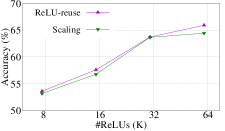
(a) ResNet18($m$=16)

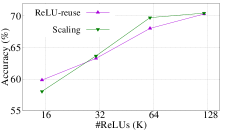
(b) ResNet18($m$=32)

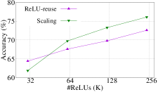
(c) ResNet18($m$=64)

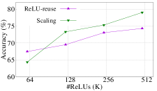
(d) ResNet18($m$=128)

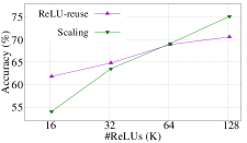
(e) 4x4x4x

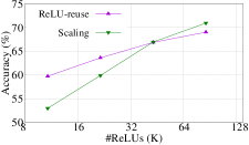
(f) HRN-2x6x2x

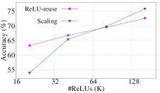
(g) HRN-5x5x3x

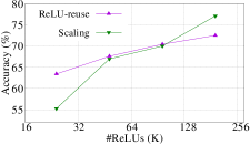
(h) HRN-6x6x2x

Figure 22: Performance comparison (CIFAR-100) of ReLU-reuse vs conventional scaling (used as reshaping steps in DeepReDuce Jha et al. (2021)) when ReLU-reuse is employed after every convolution layer.

ReLU-reuse is more effective for HybReNets and outperforms the SOTA channel-wise ReLU optimization: We examine the efficacy of ReLU-reuse on networks with various ReLUs’ distributions and compare their performance with conventional (channel/feature-map)scaling used in DeepReDuce for achieving very low ReLU counts. Results are shown in Figure 22 and Figure 23 (AppendixG). Interestingly, we observed that the efficacy of ReLU-reuse is most pronounced in networks where ReLUs are aligned in their criticality order, whether partially or entirely. In fact, networks with an even distribution of stagewise ReLUs exhibit more significant accuracy improvements from ReLU-reuse compared to traditional networks like ResNets.

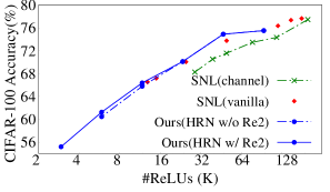
(a) HRN-2x5x2x

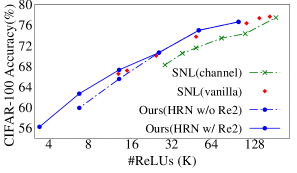
(b) HRN-2x5x3x

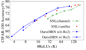
(c) HRN-2x6x2x

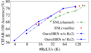
(d) HRN-2x7x2x

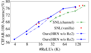
(e) HRN-2x6x3x

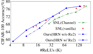
(f) HRN-2x9x2x

Figure 12: ReLU-reuse (Re2) consistently outperforms SOTA channel-wise ReLU dropping technique (SNL) by a significant margin across various ReLU counts. Accuracy gain of 1% - 3% is achieved when Re2 is substituted with the conventional scaling, as used in DeepReDuce (denoted as “w/o Re2”). This gain brings Re2 to a performance level comparable to pixel-wise SNL, denoted as “SNL(vanilla)”.

Further, we employ ReLU-reuse on HRNs with $\alpha$=2, as per Algorithm 2, and compare their performance with SOTA channel-wise ReLU optimization method used in SNL. For a fair comparison, we use standard knowledge distillation Hinton et al. (2015), as used in SNL, rather than DKD Zhao et al. (2022). Figure 12 demonstrates that Re2 results in a significant accuracy improvement of up to 3%. This gain in accuracy enables HRNs to achieve performance on par with pixel-wise SNL.

The baseline HybReNets exhibits superior ReLU efficiency compared to the standard networks used in private inference:

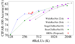
Figure 13: ReLU efficiency comparison with baseline HybReNets. For WideResNets $k\in$ {2, 4, 6, 8, 10, 12}.

We evaluated the ReLU efficiency of baseline HRNs without leveraging any coarse or fine-grained ReLU optimization methods, as well as knowledge distillation. We compared them with two widely used network architectures in PI: ResNet and WideResNets. Results are shown in Figure 13. The homogeneous channel scaling in ResNet18 StageCh networks led to superior ReLU efficiency than WideResNets variants until accuracy in the former is saturated. Nonetheless, all the four HRNs — HRN-5x5x3x, HRN-5x7x2x, HRN-6x6x2x, and HRN-7x5x2x — exceeds the ReLU efficiency of ResNet18 StageCh variants, demonstrating the benefits of strategically allocating channels in the subsequent stages of the classical networks for PI.

6 Related Work

PI-specific network optimization: Delphi Mishra et al. (2020) and SAFENet Lou et al. (2021) substitute the ReLUs with low-degree polynomials, while DeepReDuce Jha et al. (2021) is a coarse-grained ReLU optimization and drops ReLUs layerwise. SNL Cho et al. (2022b) and SENet Kundu et al. (2023a) are fine-grained ReLU optimization and drop the pixel-wise ReLUs. CryptoNAS Ghodsi et al. (2020) and Sphynx Cho et al. (2022a) use neural architecture search and employ a constant number of ReLUs per layer for designing ReLU-efficient networks, disregarding FLOPs implications. In contrast, our approach achieves ReLU and FLOP efficiency simultaneously. We refer the reader to Ng & Chow (2023) for detailed HE and GC-specific optimizations for private inference.

Benefits of width: The impact of network width on reducing catastrophic forgetting was highlighted by Mirzadeh et al. (2022). The influence of network width on the smoothness of the loss surface was analyzed by Li et al. (2018), and it was found that an increase in width could mitigate erratic behavior in the loss landscape. A study by Golubeva et al. (2021) decoupled the effects of increased width from over-parameterization and found that the width of a network primarily determines its predictive performance, with the number of parameters being a secondary factor under mild assumptions. Nguyen et al. (2021) established that wider networks, when delivering similar levels of accuracy on the ImageNet dataset, show superior performance on inputs that reflect the scene rather than the objects.

Challenges and implications of nonlinear layers in diverse neural network applications: Nonlinear layers not only present challenges in private inference; they introduce significant hurdles across various neural network applications. For instance, in the realm of optical neural networks, ReLUs exacerbate energy consumption and increase latency due to the costs associated with optical-to-electrical signal conversions, which in turn diminishes the overall system efficiency Chang et al. (2018); Li et al. (2022). When it comes to verifying adversarial robustness, the prevalence of ReLUs can make the process notably more time-intensive. This increase in complexity arises from the higher proportion of unstable neurons Xiao et al. (2019); Balunović & Vechev (2020); Chen et al. (2022a).

Additionally, ReLUs considerably hinder the progress of verifiable machine learning because its non-arithmetic operations are incompatible with zero-knowledge proof systems Sun & Zhang (2023), and prior work have resorted to employing polynomial approximations Ali et al. (2020); Zhao et al. (2021); Eisenhofer et al. (2022) or have implemented methods based on lookup tables Liu et al. (2021); Kang et al. (2022). Furthermore, the non-distributive nature of ReLU over rotation operations can break the equivariance property of Steerable CNNs Franzen & Wand (2021), known for their parameter and computation efficiency Cohen & Welling (2017); Weiler et al. (2018); Weiler & Cesa (2019); thus, limiting their architectural choices and applicability.

Thus, the ReLU optimization techniques of DeepReShape not only address the challenges in private inference but also hold promise for broader applications, suggesting its versatility and potential for widespread impact.

7 Discussion and Conclusion

Privacy-preserving computations demand substantial resources, particularly in terms of storage, communication bandwidth, and compute power. Using the garbled-circuit technique alone can consume hundreds of gigabytes of storage, while homomorphic computations might need hours to complete a single private inference in real-world scenarios Garimella et al. (2023). Earlier research has proposed specialized hardware accelerators Samardzic et al. (2021; 2022); Mo et al. (2023) and (cryptographic) protocol improvements to tackle these challenges. Yet, these solutions present challenges of their own: hardware solutions may not always be sustainable in the long run Gupta et al. (2022), and protocol tweaks could potentially open doors to security vulnerabilities or raise compatibility concerns.

In this context, our research shifts the focus towards algorithmic innovations and aims to address the unique challenge of reducing FLOPs without compromising ReLU efficiency. We proposed DeepReShape to optimize FLOP count while maintaining ReLU efficiency effectively. We achieve this by identifying superfluous FLOPs in conventional ReLU efficient networks and understanding that wide networks are mainly beneficial for higher ReLU counts, providing additional opportunities for FLOP reduction when targeting lower ReLU counts. By leveraging these insights, we achieve FLOP reduction up to 45$\times$ without any bells and whistles.

One significant advantage of algorithmic improvement lies in their adaptability across diverse hardware configurations and cryptographic protocols, thus broadening the potential impact of our algorithmic innovations. We have demonstrated that a substantial reduction in runtime, $\sim$(5$\times$ to 10$\times$), can be achieved simply by strategically allocating channels in the existing networks and employing straightforward ReLU optimization steps. It is important to note that further reductions in FLOP can be achieved by employing off-the-shelf FLOP reduction techniques. For example, techniques such as layer merging, as demonstrated in Jha et al. (2021); Dror et al. (2021); Kundu et al. (2023b) or channel pruning, as employed in SENet++ Kundu et al. (2023a). However, these approaches often sacrifice ReLU efficiency, a critical aspect of private inference.

Appendix A Rationale Behind Choosing Specific $\alpha$, $\beta$, and $\gamma$ Values in HybReNet Networks

(a) HRN-5x7x2x (Proposed)

(b) HRN-6x6x2x(Proposed)

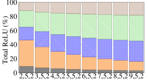
(c) HRN-7x5x2x(Proposed)

Figure 14: ReLU distribution analysis in HRN networks by progressively increasing the $\alpha$ values from $\alpha$=2, enabling a comprehensive characterization of ReLU distribution. Once the network achieves ReLU equalization – (5, 7, 2) for HRN-5x7x2x, (6, 6, 2) for HRN-6x6x2x, and (7, 5, 2) for HRN-7x5x2x – the (relative) ReLU distribution remains stable with increasing $\alpha$ value.

We chose the smallest $\alpha$ values within a specified range for the given four pairs of ($\beta$, $\gamma$) based on two primary considerations. Firstly, when the network attains ReLU equalization, the ReLU distribution becomes stable and stays constant as $\alpha$ grows. This stability stems from the fact that altering $\alpha$ has the least impact on the relative distribution of stage-wise ReLUs compared to increasing $\beta$ and $\gamma$. Specifically, increasing $\alpha$ results in a slight decrease in the proportion of Stage1 and a slight increase in the remaining stages. Secondly, when ReLU optimization (DeepReDuce) is employed, increasing alpha in HRNs does not improve the ReLU efficiency. Instead, it results in an inferior ReLU-accuracy tradeoff at lower ReLU counts (see Figure 15).

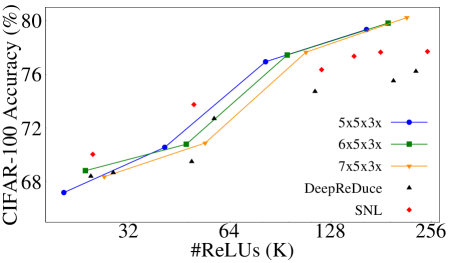
(a) HRN-5x5x3x

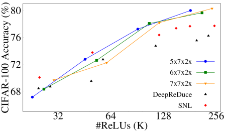
(b) HRN-5x7x2x

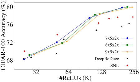
(c) HRN-7x5x2x

(d) HRN-6x6x2x

Figure 15: Effect of increasing $\alpha$ in HybeReNets: The ReLU-efficiency of networks with higher $\alpha$ does not improve, in fact it significantly reduces at lower ReLU counts.

Appendix B Impact of Network Width and Distribution of ReLUs on Their Criticality Order

Table 8: Evaluating Stagewise ReLU Criticality in ResNet18 (R18) $BaseCh$ and $StageCh$ Networks, on CIFAR-100. The criticality metric values ($C_{k}$) for each stage are determined using the Jha et al. (2021) method. Notably, the criticality order for both $BaseCh$ and $StageCh$ networks remains identical to the original ResNet18 sequence: $S_{3}>S_{2}>S_{4}>S_{1}$(Higher $C_{k}$ implies more critical ReLUs)

Networks	Stage1				Stage2				Stage3				Stage4
	#ReLUs	Acc(%)	+KD(%)	$C_{k}$	#ReLUs	Acc(%)	+KD(%)	$C_{k}$	#ReLUs	Acc(%)	+KD(%)	$C_{k}$	#ReLUs	Acc(%)	+KD(%)	$C_{k}$
R18(m=16)-2x2x2x	81.92K	52.08	52.67	0.00	32.77K	61.24	62.10	7.39	16.38K	63.00	64.64	9.84	8.19K	58.09	59.70	6.07
R18(m=32)-2x2x2x	163.84K	59.19	60.19	0.00	65.54K	65.91	66.47	4.69	32.77K	65.7	67.28	5.55	16.38K	60.48	62.22	1.67
R18(m=64)-2x2x2x	327.68K	62.65	63.13	0.00	131.07K	67.18	68.32	3.69	65.54K	68.75	70.29	5.34	32.77K	62.63	63.47	0.27
R18(m=128)-2x2x2x	655.36K	62.34	64.15	0.00	262.14K	69.28	70.56	4.34	131.07K	71.25	72.04	5.61	65.54K	63.59	64.58	0.32
R18(m=256)-2x2x2x	1310.72K	64.81	65.22	0.00	524.29K	71.95	72.43	4.65	262.14K	72.69	73.77	5.79	131.07K	64.79	65.77	0.39
R18(m=16)-3x3x3x	81.92K	52.77	53.07	0.00	49.15K	64.93	65.67	9.59	36.86K	66.23	67.96	11.57	27.65K	61.74	63.43	8.21
R18(m=16)-4x4x4x	81.92K	52.19	52.20	0.00	65.54K	65.62	66.22	10.46	65.54K	67.82	69.16	12.66	65.54K	63.52	65.46	9.89
R18(m=16)-5x5x5x	81.92K	50.38	50.65	0.00	81.92K	66.10	66.63	11.74	102.40K	70.17	70.64	14.46	128.00K	64.86	65.43	10.52
R18(m=16)-6x6x6x	81.92K	50.60	51.53	0.00	98.30K	66.74	67.11	11.30	147.46K	70.67	72.09	14.49	221.18K	65.22	66.43	10.21
R18(m=16)-7x7x7x	81.92K	50.93	49.07	0.00	114.69K	66.59	67.89	13.50	200.70K	72.08	73.33	16.74	351.23K	65.95	67.88	12.48

It remains intriguing to examine if the ReLUs’ criticality order in baseline networks, such as ResNet18, remains consistent when the network width is modified, specifically in the $BaseCh$, StageCh, and HRN variations. To this end, we compute the stagewise criticality metric for ResNet18 $BaseCh$ and StageCh networks (Table 8), and HRN networks with $\alpha$ values between 2 and 7 (Table 9. Interestingly, the criticality order of the standard ResNet18 is preserved in $BaseCh$ and StageCh models, and all HRNs, except for those with $\alpha$=2 (HRN-2x5x3x, HRN-2x5x2x, HRN-2x6x2x, and HRN-2x7x2x). Specifically, the criticality order of Stage2 and Stage3 is shuffled in HRNs with $\alpha$=2, while the most and least critical stages remain unchanged (i.e., $S_{3}>S_{2}>S_{4}>S_{1}$). To account for this altered criticality order, we recompute $\alpha$, $\beta$, and $\gamma$ using Algorithm 1, and obtain two HRNs, HRN-2x6x3x and HRN-2x9x2x; however, the criticality order in these two HRNs does not adapt to the altered criticality order (highlighted as green in Table 9).

Table 9: Evaluating Stagewise ReLU criticality in (ResNet18-based) HRN networks with $\alpha$ values spanning 2 to 7, on the CIFAR-100 dataset. Criticality metrics ($C_{k}$) for each stage are determined using the method in Jha et al. (2021). Notably, the criticality order of all HRN networks, except the smallest one with $\alpha$=2, aligns with the original ResNet18 order ($S_{3}>S_{2}>S_{4}>S_{1}$). HRNs with the minimum $\alpha$, $\beta$, and $\gamma$ required for (full) ReLU equalization are emphasized in gray.

Networks	Stage1				Stage2				Stage3				Stage4
	#ReLUs	Acc(%)	+KD(%)	$C_{k}$	#ReLUs	Acc(%)	+KD(%)	$C_{k}$	#ReLUs	Acc(%)	+KD(%)	$C_{k}$	#ReLUs	Acc(%)	+KD(%)	$C_{k}$
HRN-2x7x2x	81.92K	52.14	53.39	0.00	32.77K	61.63	61.59	6.42	57.34K	68.44	69.82	12.37	28.67K	62.15	63.40	7.91
HRN-3x7x2x	81.92K	51.61	53.29	0.00	49.15K	64.46	65.26	9.11	86.02K	69.88	70.77	12.80	43.01K	63.10	64.17	8.36
HRN-4x7x2x	81.92K	51.28	49.42	0.00	65.54k	65.93	66.47	12.72	114.69K	70.94	72.16	16.32	57.34K	63.70	64.77	11.56
HRN-5x7x2x	81.92K	49.82	48.36	0.00	81.92K	66.17	67.59	14.13	143.36K	71.40	72.18	16.83	71.68K	64.10	65.35	12.60
HRN-6x7x2x	81.92K	51.23	48.48	0.00	98.30K	66.88	68.06	14.20	172.03K	71.86	72.73	16.91	86.02K	64.15	65.75	12.64
HRN-7x7x2x	81.92K	50.11	52.40	0.00	114.69K	66.92	68.29	11.40	200.70K	71.69	73.16	14.32	100.35K	63.82	65.53	9.51
HRN-2x6x2x	81.92K	52.29	53.19	0.00	32.77K	61.62	62.00	6.90	49.15K	67.36	69.51	12.43	24.58K	61.64	63.25	8.04
HRN-3x6x2x	81.92K	52.50	52.80	0.00	49.15K	64.50	65.64	9.78	73.73K	68.61	70.96	13.44	36.86K	62.77	64.09	8.77
HRN-4x6x2x	81.92K	53.23	53.32	0.00	65.54K	65.74	66.03	9.48	98.30K	70.47	71.54	13.22	49.15K	63.59	64.82	8.76
HRN-5x6x2x	81.92K	50.79	51.64	0.00	81.92K	66.89	67.27	11.48	122.88K	70.33	71.50	14.18	61.44K	63.97	64.94	9.97
HRN-6x6x2x	81.92K	50.01	50.59	0.00	98.30K	66.57	67.94	12.58	147.46K	71.18	72.59	15.51	73.73K	64.13	65.39	10.95
HRN-7x6x2x	81.92K	51.01	49.64	0.00	114.69K	66.74	68.57	13.58	172.03K	71.84	72.84	16.18	86.02K	64.54	65.16	11.36
HRN-2x5x2x	81.92K	52.03	53.05	0.00	32.77K	61.60	61.76	6.82	40.96K	66.64	68.29	11.75	20.48K	61.02	62.58	7.71
HRN-3x5x2x	81.92K	53.43	52.61	0.00	49.15K	64.57	65.71	9.97	61.44K	68.40	69.93	12.98	30.72K	62.32	63.42	8.51
HRN-4x5x2x	81.92K	52.65	52.33	0.00	65.54K	65.60	66.89	10.86	81.92K	69.81	70.85	13.61	40.96K	63.14	63.94	8.95
HRN-5x5x2x	81.92K	49.15	51.16	0.00	81.92K	66.26	67.47	11.98	102.40K	70.15	71.69	14.85	51.20K	63.55	64.67	10.26
HRN-6x5x2x	81.92K	49.06	52.10	0.00	98.30K	66.56	68.08	11.59	122.88K	71.33	71.85	14.10	61.44K	63.59	64.89	9.59
HRN-7x5x2x	81.92K	51.58	51.93	0.00	114.69K	66.94	67.89	11.45	143.36K	70.79	72.87	14.79	71.68K	64.02	65.23	9.86
HRN-2x5x3x	81.92K	52.36	53.68	0.00	32.77K	61.39	61.30	5.97	40.96K	66.78	68.17	11.17	30.72K	62.01	63.83	7.99
HRN-3x5x3x	81.92K	51.05	52.89	0.00	49.15K	64.64	65.10	9.30	61.44K	68.87	70.14	12.93	46.08K	63.66	64.32	8.74
HRN-4x5x3x	81.92K	51.57	50.62	0.00	65.54K	65.66	66.06	11.52	81.92K	69.12	70.13	14.33	61.44K	63.64	65.58	11.21
HRN-5x5x3x	81.92K	50.22	52.41	0.00	81.92K	66.42	67.55	11.12	102.40K	70.15	70.97	13.42	76.80K	64.21	65.59	9.73
HRN-6x5x3x	81.92K	50.28	50.45	0.00	98.30K	65.95	67.61	12.45	122.88K	70.68	71.29	14.88	92.16K	64.37	65.87	11.23
HRN-7x5x3x	81.92K	50.12	50.31	0.00	114.69K	66.85	67.95	12.66	143.36K	71.20	71.87	15.23	107.52K	64.72	65.58	11.01
HRN-2x9x2x	81.92K	51.86	53.22	0.00	32.77K	61.13	61.65	6.60	73.73K	69.46	70.28	12.63	36.86K	62.53	64.25	8.57
HRN-2x6x3x	81.92K	52.75	52.85	0.00	32.77K	61.33	61.44	6.73	49.15K	67.36	68.76	12.11	36.86K	62.69	64.59	9.12

Appendix C Additional Experimental Results

C.1 ReLU Equalization through Network’s Depth in BaseCh Networks

ReLU equalization through width in HybReNets results in two simultaneous effects. Firstly, it increases the network’s complexity per unit of nonlinearity, measured as parameters and FLOPs per unit of ReLU. Secondly, it aligns the distribution of ReLUs in their criticality order. However, to analyze the significance of these effects independently, we apply ReLU equalization through depth and augment the base channel counts to increase the parameters and FLOPs per unit of ReLU.

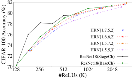
(a) ReLU-efficiency comparison

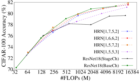
(b) FLOPs-efficiency comparison

Figure 16: ReLU and FLOPs efficiency when network’s ReLU is equalized, in their criticality order, through depth, by altering the stage compute ratios (their modified values are shown in bracket []). The network’s complexity per units of nonlinearity (ReLUs) is increased by augmenting $m\in\{16,32,64,128,256\}$. ReLU and FLOPs efficiency of these HRNs are either similar or worse compared to $BaseCh$ networks, suggesting the effectiveness of ReLU equalization through width (by altering $\alpha$, $\beta$, and $\gamma$)

In this study, we use the classical ResNet18 with $m$=16 and fixed $\alpha$=$\beta$=$\gamma$=2; however, set the stage compute ratios ($\phi_{1}$, $\phi_{2}$, $\phi_{3}$, and $\phi_{4}$) as design hyperparameters. Now, we employ Algorithm 1 for ReLU equalization and solve compound inequalities to obtain the depth hyperparameters. Specifically, we determine the depth hyperparameters ($\phi_{1}$, $\phi_{2}$, $\phi_{3}$, $\phi_{4}$) $\in$ {(1,5,5,3); (1,5,7,2); (1,6,6,2); and (1,7,5,2)} that correspond to the minimum values enabling ReLU equalization. It is worth noting that the sum of all the stage compute ratios results in a network’s global depth of 14. Next, we increase the parameters and FLOPs per unit of ReLU by varying $m$ $\in$ {16, 32, 64, 128, and 256}. The experimental results are shown in Figure 16, where we compare the ReLU and FLOPs efficiency with $BaseCh$ and StageCh networks. Interestingly, we observe that the ReLU and FLOPs efficiency of the networks derived above are either similar or worse compared to BaseCh networks. For instance, HRN[1,5,5,3] exhibits inferior ReLU/FLOPs efficiency at higher ReLU/FLOPs count compared with BaseCh networks. Consequently, this underscores the significance of ReLU equalization through width adjustment by altering $\alpha$, $\beta$, and $\gamma$, and demonstrates that ReLU equalization alone does not yield the desired benefits in HybReNets.

C.2 Additional Results for Capacity-Criticality-Tradeoff

We conducted additional experiments on different HybReNets to investigate further the “Capacity-Criticality Tradeoff” phenomenon shown in Figure 6. In particular, for each set of experiments, we chose three HRN networks with reduced values of $\alpha$ and a fixed ($\beta$,$\gamma$) and employed DeepReDuce and SNL ReLU optimization techniques. The results are presented in Figure 17. Notably, lowering $\alpha$ results in a higher fraction of the network’s ReLUs in Stage1, as shown in Table 9. For instance, HRN-6x6x2x, HRN-4x6x2x, and HRN-2x6x2x have the Stage1 fraction of the network’s total ReLU count as 20.4%, 27.8%, and 43.5%, respectively. Our observations on DeepReDuce and SNL are consistent with those in Figure 6. Precisely, HRN-6x6x2x and HRN-4x6x2x outperform HRN-2x6x2x at higher ReLU counts, whereas HRN-2x6x2x is superior at lower ReLU counts (Figure 17(b,e)).

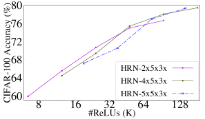
(a) DeepReDuce on HRN-5x5x3x

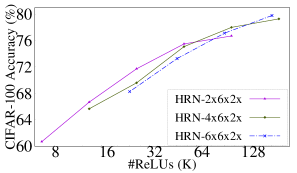
(b) DeepReDuce on HRN-6x6x2x

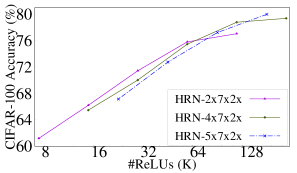
(c) DeepReDuce on HRN-5x7x2x

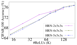
(d) SNL on HRN-5x5x3x

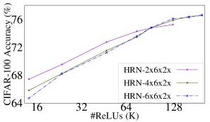
(e) SNL on HRN-6x6x2x

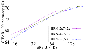
(f) SNL on HRN-5x7x2x

Figure 17: Capacity-Criticality Tradeoff in HRN networks for coarse/fine-grained ReLU optimization DeepReDuce/SNL. HRN networks with decreasing value of $\alpha$ has higher proportion of Stage1 (least-critical) ReLUs, and exhibit superior performance at lower ReLU counts.

C.3 Explanation and Intuition for Capacity-Criticality Tradeoff

We have observed that networks with a higher percentage of least-critical (Stage1) ReLUs tend to have lower overall ReLU counts. This pattern is consistent across traditional networks like ResNet18 and WRN22x8, as well as HRN networks. For example, WRN22x8 and ResNet18, used in SNL Cho et al. (2022b) and SENet Kundu et al. (2023a) for advancing the ReLU-accuracy Pareto frontier at different ReLU counts, contain 1392.6K and 557K ReLUs, respectively. Also, in HybReNet, when we decrease the value of $\alpha$ while keeping $\beta$ and $\gamma$, the total ReLU count in the network decreases, and the percentage of Stage1 ReLUs increases. For instance, HRN-6x6x2x, HRN-4x6x2x, and HRN-2x6x2x have ReLU counts of 401.4K, 294.9K, and 188.4K, respectively. This raises the fundamental question of what drives the better performance at lower ReLU counts — the proportion of ReLUs in Stage1 or the total number of ReLUs in the network? Further investigation is required to shed light on this issue.

To pinpoint the primary factor influencing PI performance at lower ReLU counts, we conducted an experiment with ResNet34 and a ResNet18 variant (ResNet18($m=16$)-4x4x4x), having a uniform ReLU distribution, as employed in Ghodsi et al. (2020) and Sphynx Cho et al. (2022a). Results are shown in Table 10. Despite having 3.5$\times$ fewer ReLUs, the performance of ResNet18($m$=16)-4x4x4x is inferior to that of ResNet34 when ReLU counts are below 50K. This is due to a lower percentage (29.41%) of Stage1 ReLUs in comparison to ResNet34 (47.46%). Likewise, the improved performance of ResNet18 over WRN22x8 at lower ReLU counts, as seen in previous studies Kundu et al. (2023a); Cho et al. (2022b), cannot be ascribed to the total ReLU count. Instead, it is attributed to the proportion of Stage1 ReLUs, with ResNet18 having 58.8% and WRN22x8 having 48.2%.

Network	#ReLUs	Stage1(%)	180K	100K	50K	15K
ResNet34	966.7K	47.46	76.35%	74.55%	72.07%	66.46%
4x4x4x	278.5K	29.41	77.08%	75.03%	71.38%	64.77%

Table 10: Performance comparison (using SNL ReLU optimization) of ResNet34 and ResNet18 variant (ResNet18($m$=16)-4x4x4x), having a uniform distribution of ReLUs. Stage1(%) is the fraction of network’s ReLU in Stage1. Despite having 3.5$\times$ fewer ReLUs, the performance of 4x4x4x remains inferior to ResNet34 when the ReLU count falls below 50K. Thus, the key determinant for the superior performance at very low ReLU count is the fraction of least-critical ReLUs, rather than the network’s total ReLU count.

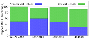
Figure 18: Networks with higher fraction of least-critical (Stage1) ReLUs, ResNet18 (ResNet34) drops lesser fraction of their (remaining stages) critical ReLUs, compared to WRN22x8 (4x4x4x), to achieve a ReLU count of 25K, regardless of the their absolute ReLU counts.

To better understand why having a higher fraction of Stage1 ReLUs is preferable for achieving superior performance at lower ReLU counts, we examined the ReLU dropping strategies employed in the prevalent ReLU optimization techniques. Specifically, we discussed the strategies used by DeepReDuce Jha et al. (2021), SNL Cho et al. (2022b), and SENet Kundu et al. (2023a), and found that they consistently demonstrate that Stage1 ReLUs are the least critical, and as such, all Stage1 ReLUs are dropped first to achieve very low ReLU counts. Consequently, networks with a greater proportion of least-critical ReLUs will drop a lower fraction of their critical ReLUs when aiming for very low ReLU counts, as opposed to networks with a lower proportion of least-critical ReLUs. This can be observed in Figure 18. In particular, regardless of the total ReLU count of the network, WRN22x8 (ResNet18($m$=16)-4x4x4x) drops a higher fraction of their critical ReLUs compared to ResNet18 (ResNet34) to attain a ReLU count of 25K. Thus, dropping a higher fraction of critical ReLUs leads to a significant loss in accuracy and results in inferior performance.

Further, we note that the observation as mentioned above resonates with the findings made in Yosinski et al. (2014) — neurons in the middle layers of a network (i.e., Stage2 and Stage3) exhibit fragile co-adaption, which is challenging to re-learn. Consequently, dropping more ReLUs from these stages in a network with a lower fraction of least-critical (Stage1) ReLUs would disrupt the fragile co-adaption and significantly reduce performance.

C.4 SNL ReLU Optimization on HybReNet Networks

We employ SNL ReLU optimization Cho et al. (2022b) on the four distinct HRN configurations – HRN-5x5x3x, HRN-5x7x2x, HRN-6x6x2x, and HRN-7x5x2x – to assess the efficacy of fine-grained ReLU optimization in the context of HRNs. Results are presented in Figure 19. Evidently, the HRNs with SNL ReLU optimization are inferior to the vanilla SNL, employed on WRN22x8 (for #ReLUs $>$ 100K) and ResNet18 (for #ReLUs $\leq$ 100K). However, employing SNL on ReLU-Thinned HRNs results in an accuracy boost, up to 3%, across all the ReLU counts. This leads to at-par performance with vanilla SNL, thereby emphasizing the significance of ReLU Thinning even for the fine-grained ReLU optimization.

Notice that the aforementioned findings are consistent with the observations made in Figure 7 and Table 4, demonstrating the limitations of SNL when the distribution of ReLU altered. Specifically, when the proportion of the network’s ReLU belonging to Stage1 decreases and those in the other stages increase. This implies that the benefits of fine-grained ReLU optimization may be contingent on a higher proportion of least-critical (Stage1) ReLUs. Further, to assess the efficacy of ReLU Thinning in the context of fine-grained ReLU optimization, we compare the total number of ReLUs within a network before and after the implementation of the technique. For instance, in the case of a 50K ReLU budget allocated to the HRN-5x7x2x model, the SNL algorithm identifies 50K essential ReLUs from an initial pool of 363.5K ReLUs, subsequently eliminating 312.5K ReLUs. Conversely, when employing the Thinned HRN network, the SNL algorithm detects the 50K critical ReLUs from a diminished pool of 181.25K ReLUs and drops 131.25K ReLUs, given that Thinning eliminates half of the network’s ReLUs from alternating layers, irrespective of their criticality. This results into an accuracy boost of 2.44% (on CIFAR-100). Thus, ReLU Thinning effectively reduces the search space required to identify critical ReLUs.

(a) HRN-5x5x3x

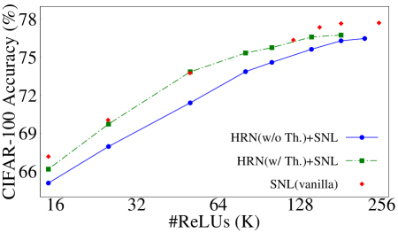
(b) HRN-5x7x2x

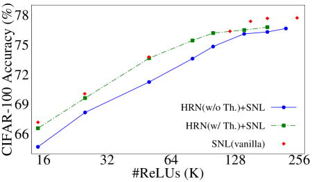
(c) HRN-6x6x2x

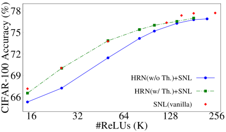
(d) HRN-7x5x2x

Figure 19: HybReNets with fine-grained ReLU optimization: HRNs with SNL (fine-grained) ReLU optimization exhibit a suboptimal ReLU-Accuracy tradeoff compared to the vanilla SNL approach used in traditional networks such as ResNet18 and WRN22x8. However, employing ReLU-Thinning (a coarse-grained ReLU optimization step used in DeepReDuce), prior to SNL optimization yields performance on par with the vanilla SNL method, thus highlighting the significance of ReLU Thinning in ReLU optimization, even in the context of fine-grained ReLU optimization.

Appendix D Detailed Analysis of ReLU-Accuracy Pareto Points

In this section, we detailed the ReLU optimization steps used in the ReLU-Accuracy Pareto frontier, transitioning from higher to lower accuracy points, as shown in Figure 11 (a,b) and the Table 6. When employing ReLU-reuse, we fixed $m$=16; however, the network’s FLOPs count reduces due to the group-wise convolution. For instance, the HRN-2x6x3x model with a ReLU-reuse factor of four has 370.1M FLOPs, compared to the original HRN-2x6x3x model ($m$=16) with 527.4M FLOPs, when used on CIFAR-100 (see Table 12). Nonetheless, because of specific implementation constraints of group convolution in Microsoft SEAL SEAL , we calculated the HE latency without considering the FLOP reduction resulting from group convolution in ReLU-reuse.

Table 11: Network configurations and ReLU optimization steps employed for the HybReNet points in Table 6. Accuracies (TinyImageNet) are separately shown for vanilla KD Hinton et al. (2015) and DKD Zhao et al. (2022), highlighting the benefits of improved architectural design and distillation method.Re2 denotes ReLU-reuse, and used for efficient PI at very low ReLU counts.

HybReNet	$m$	ReLU optimization steps			#ReLU	#FLOPs	Accuracy(%)		Acc./ReLU
		Culled	Thinned	Re2			KD	DKD
5x5x3x	16	NA	S1+S2+S3+S4	NA	653.3K	4216.4M	65.76	67.58	0.10
2x5x3x	32	S1	S2+S3+S4	NA	417.8K	2841.7M	64.11	66.10	0.16
5x5x3x	8	NA	S1+S2+S3+S4	NA	326.6K	1055.4M	61.92	64.92	0.20
2x5x3x	8	S1	S2+S3+S4	NA	104.4K	178.9M	56.37	58.90	0.56
2x5x3x	16	S1	S2+S3+S4	4	52.2K	486.3M	53.13	54.46	1.04

Table 12: Network configurations and ReLU optimization steps employed for the Pareto points in Figure 11 (a,b), along with and the HybReNet points used for the comparison with SOTA PI methods and ConvNeXt-V2 Woo et al. (2023) as illustrated in Table 12. Re2 denotes ReLU-reuse, a key method in achieving significantly reduced ReLU-counts.

		Nets	m	ReLU optimization steps			#ReLU	#FLOPs	Accuracy(%)		Acc./ReLU
				Culled	Thinned	Re2			KD	DKD
CIFAR-100	HybReNet	4x6x3x	16	NA	S1+S2+S3+S4	NA	317.4K	2061.1M	80.14	81.36	0.26
		2x6x3x	16	S1	S2+S3+S4	NA	134.1K	527.4M	78.80	79.56	0.59
		2x6x3x	8	S1	S2+S3+S4	NA	67.1K	132.2M	74.84	76.91	1.15
		2x6x3x	16	S1	S2+S3+S4	4	33.5K	370.1M	70.93	73.89	2.21
		2x6x3x	16	S1	S2+S3+S4	8	16.6K	394.8M	68.17	69.70	4.19
		2x6x3x	16	S1	S2+S3+S4	16	8.3K	413.4M	62.44	64.65	7.78
TinyImageNet	HybReNet	4x6x3x	16	NA	S1+S2+S3+S4	NA	1269.8K	8244.2M	68.90	70.29	0.06
		4x6x3x	12	NA	S1+S2+S3+S4	NA	952K	4638.8M	68.16	69.15	0.07
		2x6x3x	16	S1	S2+S3+S4	NA	536.6K	2109.4M	66.29	67.48	0.13
		2x6x3x	12	S1	S2+S3+S4	NA	402K	1187.5M	64.51	65.77	0.16
		2x6x3x	8	S1	S2+S3+S4	NA	268.3K	528.6M	60.97	64.02	0.24
		2x6x3x	16	S1	S2+S3+S4	4	134.1K	1480.1M	57.84	61.52	0.46
		2x6x3x	16	S1	S2+S3+S4	8	67.1K	1579.2M	54.47	56.24	0.84
		2x6x3x	16	S1	S2+S3+S4	16	33.5K	1653.5M	49.13	49.96	1.49
	ConvNeXt	T	96	S1	S2+S3+S4	NA	1622K	11801M	68.32	69.85	0.04
		N	80	S1	S2+S3+S4	NA	1278K	9080.2M	66.73	68.75	0.05
		P	64	S1	S2+S3+S4	NA	720.9K	3435.7M	65.42	67.08	0.09
		F	48	S1	S2+S3+S4	NA	540.7K	1935M	64.23	65.72	0.12
		A	40	S1	S2+S3+S4	NA	450.6K	1345.1M	63.23	64.08	0.14

Appendix E Discussion

E.1 FLOP efficiency Restricts the Flexibility for Widening Classical Neural Networks

Classical networks follow a convention of doubling the filter count when downsampling feature maps by a factor of two to avoid representational bottlenecks Szegedy et al. (2016). This results in a fixed stagewise channel multiplication factor (shown in Figure 2) of $\alpha=\beta=\gamma=2$ for most classical networks. Even for designing sate-of-the-art FLOPs-efficient vision models, RegNet Radosavovic et al. (2020), stagewise channel multiplication factor are restricted as $1.5\leq$($\alpha$, $\beta$, $\gamma$) $\leq 3$. Conventional network design paradigms prioritize FLOP efficiency, so the stagewise multiplication factor is typically conservative. The quadratic dependency of FLOPs on the channel counts (see Figure 2), along with the multiplicative effect of stagewise multiplication factors, means that even a small increase in these factors can lead to a significant increase in FLOPs count, thus hampering FLOPs efficiency.

In contrast, we observed that networks having a higher value of $\beta$, along with lower values of $\alpha$ and $\gamma$, provide a better ReLU-FLOP-Accuracy tradeoff compared to the classical networks with $\alpha=\beta=\gamma=2$. Notably, HRN-2x5x2x, HRN-2x5x2x, HRN-2x6x2x, and HRN-2x7x2x outperform ResNet18 baseline networks, with both $m$=64 and $m$=32, and exhibit a better ReLU-FLOP-Accuracy balance.

E.2 Regulating FLOPs in Deeper Layers of HybReNets

The derivation steps for ReLU equalization on a four-stage network show that $\beta$ and $\gamma$ values are bounded by $\beta\gamma<16$ and $\gamma<4$. These constraints effectively limit the growth of FLOPs in deeper layers, making HRN networks more efficient in terms of computation than their StageCh counterparts, which exhibit homogeneous sets of $\alpha$, $\beta$, and $\gamma$, leading to an undesirably rapid growth of FLOPs in deeper layers. To visualize this, we compute the normalized FLOPs in ResNet18-based StageCh networks, contrasting with HRNs. We observed that the normalized FLOPs in Stage3 and Stage4 of ResNet18 are expressed as $\frac{\alpha^{2}\beta^{2}}{16}$ and $\frac{\alpha^{2}\beta^{2}\gamma^{2}}{64}$ (respectively); thus, network with $\gamma$=2 would have equal FLOPs in Stage3 and Stage4. This is evident from the (normalized) stagewise FLOPs ratio for HRN-5x7x2x, HRN-7x5x2x, and HRN-6x6x2x networks in Table 13.

Table 13: Depiction of stagewise FLOPs and ReLU trend variation, with $\alpha$,$\beta$, and $\gamma$, in StageCh and HRN networks. The least and most critical ReLUs are colored in red and blue, respectively. Evidently, in constrast with StageCh network, ReLU-equalization in HRNs restrict the growth of FLOPs in deeper layers and networks achieve ReLU efficiency at par with StageCh network; however, with fewer FLOPs. This way HRN networks achieve ReLU-FLOP-Accuracy balance.

	Stage1	Stage2	Stage3	Stage4		($\alpha,\beta,\gamma$)=2	2$<$($\alpha,\beta,\gamma$)$<$4	($\alpha,\beta,\gamma$)=$4$	($\alpha,\beta,\gamma$)$>$4
FLOPs	1	$\frac{\alpha^{2}}{4}$	$\frac{\alpha^{2}\beta^{2}}{16}$	$\frac{\alpha^{2}\beta^{2}\gamma^{2}}{64}$	Layerwise FLOPs	constant	increasing ($\uparrow$)	increasing ($\uparrow\uparrow$)	increasing ($\uparrow\uparrow\uparrow$)
ReLUs	1	$\frac{\alpha}{4}$	$\frac{\alpha\beta}{16}$	$\frac{\alpha\beta\gamma}{64}$	Layerwise ReLUs	decreasing ($\downarrow\downarrow$)	decreasing ($\downarrow$)	constant	increasing ($\uparrow$)

	($\alpha,\beta,\gamma$) = (2, 2, 2)				($\alpha,\beta,\gamma$) = (3, 3, 3)				($\alpha,\beta,\gamma$) = (4, 4, 4)				($\alpha,\beta,\gamma$) = (6, 6, 6)
	Stage1	Stage2	Stage3	Stage4	Stage1	Stage2	Stage3	Stage4	Stage1	Stage2	Stage3	Stage4	Stage1	Stage2	Stage3	Stage4
FLOPs	64	64	64	64	64	144	324	729	64	256	1024	4096	64	576	5184	46656
ReLUs	64	32	16	8	64	48	36	27	64	64	64	64	64	96	144	216
	HRN-5x7x2x				HRN-7x5x2x				HRN-6x6x2x				HRN-5x5x3x
	Stage1	Stage2	Stage3	Stage4	Stage1	Stage2	Stage3	Stage4	Stage1	Stage2	Stage3	Stage4	Stage1	Stage2	Stage3	Stage4
FLOPs	64	400	4900	4900	64	784	4900	4900	64	576	5184	5184	64	400	2500	5625
ReLUs	64	80	140	70	64	112	140	70	64	96	144	72	64	80	100	75

In conclusion, constraints on $\gamma$, which must be less than 4, keep the ReLU count of Stage4 lower than that of Stage3 (most critical stage), which in turn restricts the FLOPs count of Stage4. While further limiting $\alpha$ and $\beta$ values can reduce the network’s FLOPs, this would also reduce the proportion of the most significant (Stage3) ReLUs. As a result, a criticality-aware network design streamlines both the ReLU and FLOPs in networks, prevents superfluous FLOPs (in contrast with StageCh networks), and maximizes the utilization of the network’s FLOPs for a given ReLU count.

E.3 Understanding Accuracy Plateau in Homogeneous Channel Scaling through the Deep Double Descent Phenomenon

A distinct trend in the ReLU-Accuracy tradeoff has been observed (see Figure 3(a,b))as the width of models is increased by augmenting $\alpha$, $\beta$, and $\gamma$. Specifically, accuracy initially increases with increasing values of $\alpha$, $\beta$, and $\gamma$, reaches a saturation point, then increases again at higher ReLU counts. This trend is more prominent in models with smaller depth, such as ResNet18, and disappears in deeper models, like ResNet56, where performance does not improve after saturation. The observed saturation trend in ReLU-accuracy tradeoff can be explained by the “model-wise deep double descent” phenomenon, which becomes more pronounced with higher label noise Belkin et al. (2019); Nakkiran et al. (2021); Somepalli et al. (2022). In the presence of label noise, a U-shaped curve appears in the classical (under-parameterized) regime due to a bias-variance tradeoff. In the over-parameterized regime, accuracy improves due to the regularization enabled by the strong inductive bias of the network. However, with zero label noise, the test error plateaus around the interpolation threshold, resulting in a flat trend similar to the one shown in Figure 3(a,b) instead of a U-shaped curve.

E.4 Why RegNet and ConvNeXt Models are Selected for Our Case Study?

RegNets are models that have been designed using a semi-automated network design method, which is parameterized by the stage compute ratio ($\phi_{1}$, $\phi_{2}$, $\phi_{3}$, $\phi_{4}$), base channel count ($m$), and stagewise channel multiplication factors as $1.5\leq$($\alpha$, $\beta$, $\gamma$)$\leq 3$. On the other hand, ConvNeXts are redesigned ResNets with modified values of $m$ and $\phi_{1}$, $\phi_{2}$, $\phi_{3}$, $\phi_{4}$. For example, the ConvNeXt-T model has a stage compute ratio of [3, 3, 9, 3], which is different from the [3, 4, 6, 3] ratio used in ResNet34, and a base channel count of $m$=96, which is higher than the $m$=64 used in ResNet34. As a result, the unconstrained design choices in RegNets and the modified depth and width in ConvNeXt models make them suitable for our case study, where we investigate their impact on ReLUs’ distribution and the ReLU-FLOP-Accuracy balance.

Note that the original ConvNeXt model utilizes PI-unfriendly GeLU activation function and LayerNorm normalization, which often require approximation in ciphertext Fan et al. (2022). Therefore, we adapted the ResNets models to incorporate ConvNeXt features, specifically the stagewise channel distribution and the stage compute ratio from ConvNeXt models. Likewise, for experiments with RegNets, we opted for the RegNet-x variant instead of RegNet-y because the latter employs a sigmoid activation function in its squeeze-and-excitation blocks.

E.5 Potential of ReLU Equalization as a Unified Network Design Principle

The field of deep learning has witnessed remarkable progress in recent years, primarily due to the development of increasingly sophisticated neural network architectures. Traditionally, researchers have relied on manual network design techniques such as ResNet He et al. (2016), ResNeXt Xie et al. (2017), ConvNeXt Liu et al. (2022), etc., or neural architecture search methods Liu et al. (2018); Tan & Le (2019); Howard et al. (2019); Tan et al. (2019). However, these approaches have their limitations. Manual techniques often lead to suboptimal models as design choices increase, while neural architecture search needs to be more interpretable and may not generalize beyond restricted settings. Additionally, both methods require significant computational resources to find optimal design hyper-parameters when networks are designed from scratch.

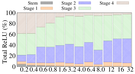
(a) RegNet-X

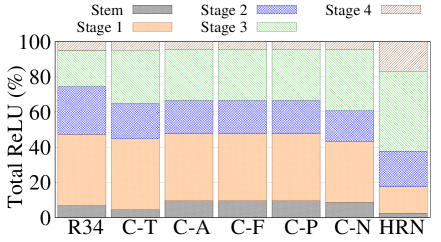
(b) ResNet34 and ConvNeXt-V2

Figure 20: Analyzing the distribution of ReLU in RegNet-X Radosavovic et al. (2020) and ConvNeXt-V2 Woo et al. (2023) architectures reveals interesting patterns. In all RegNet-X models, ReLUs are arranged precisely according to their criticality order. In contrast, the ConvNeXt models, including their T, A, F, P, and N variations, have a higher proportion of network’s ReLU in the most-critical stage (Stage3), while that of the less crucial ReLUs (Stage1) is reduced due to the modification of depth and width design parameters. In contrast, the distribution of ReLUs in the HRN-4x6x3x model strictly adheres to their criticality order.

A semi-automated design technique like RegNets Radosavovic et al. (2020) offers interpretable network design and automates the process of finding the optimal population of networks that can generalize across a wide range of settings. However, it requires training thousands of models in each iteration to narrow down the search space and assess the quality of the design space, making it expensive when models are designed from scratch. Here, we emphasize that RegNet networks’ width and depth are explained by a sophisticated quantized linear function that equalizes the networks’ ReLU in their order of criticality (see Figure 20(a)).

Likewise, ReLUs’ distribution in all but Stage1 of ConvNeXt models follows their criticality order. Precisely, the ConvNeXt-T (ConvNext-N) model increases the proportion of most-critical (Stage3) ReLUs from 20.3% to 30.2%(34.8%) in ResNet34 while reducing the proportion of less critical ReLUs (see Figure 20(b)). Furthermore, as evident from the comparative summary of stagewise channel allocation in ConvNeXt models and HRNs (with $\alpha$=2), the channel counts in the deeper stages of both models (ConvNeXt and HRNs) are an exact match, where HRNs tend to allocate fewer channels during the initial stages. This demonstrates the generality of ReLU equalization as a design principle, even for designing FLOPs-efficient models.

• ConvNext V2-T $m$=96 [96, 192, 384, 768]

• ConvNext V2-N $m$=80 [80, 160, 320, 640]

• ConvNext V2-P $m$=64 [64, 128, 256, 512]

• ConvNext V2-F $m$=48 [48, 96, 192, 384]

• ConvNext V2-A $m$=40 [40, 80, 160, 320]

• HRN-2x6x2x $m$=32 [32, 64, 384, 768]

• HRN-2x5x2x $m$=32 [32, 64, 320, 640]

• HRN-2x5x3x $m$=16 [16, 32, 160, 480]

• HRN-2x6x2x $m$=16 [16, 32, 192, 384]

• HRN-2x5x2x $m$=16 [16, 32, 160, 320]

Conclusively, ReLU-equalization only needs prior knowledge of the stagewise criticality of the baseline network, which is often the same for a specific model family and, therefore, requires training very few models. Furthermore, ReLU-equalization can be used to design both FLOPs and ReLU efficient neural networks. Thus, going forward, ReLU equalization may offer a new perspective to simplify network design for both FLOPs and ReLU efficient networks and improve interpretability.

Appendix F HybReNet with Different Criticality Order

In this paper, we perform an exhaustive characterization of HRN networks designed for the prevalent criticality order: Stage3 $>$ Stage2 $>$ Stage4 $>$ Stage1. However, we have observed that the criticality order of Stage2 and Stage4 can change in some instances, such as when using HRNs with $\alpha$=2 designed for Stage3 $>$ Stage2 $>$ Stage4 $>$ Stage1 criticality order, or when using ResNet18/ResNet34 on TinyImageNet Jha et al. (2021). In these cases, the criticality order changes to Stage3 $>$ Stage4 $>$ Stage2 $>$ Stage1. This leads to the question of whether it is necessary to run the criticality test for every baseline network on different datasets. To answer this, we need to compare the ReLU-accuracy performance of HRN networks designed with the two different criticality orders. To accomplish this, we use the DeepReShape algorithm 1 to design HybReNets for the given criticality order of Stage3 $>$ Stage4 $>$ Stage2 $>$ Stage1.

$$\#ReLUs(S_{3})>\#ReLUs(S_{4})>\#ReLUs(S_{2})>\#ReLUs(S_{1})$$

$$\implies\phi_{3}\Big{(}\frac{\alpha\beta}{16}\Big{)}>\phi_{4}\Big{(}\frac{\alpha\beta\gamma}{64}\Big{)}>\phi_{2}\Big{(}\frac{\alpha}{4}\Big{)}>\phi_{1}$$

$$\text{ReLU equalization through width}\;(\phi_{1}=\phi_{2}=\phi_{3}=\phi_{4}=2,\;\text{and}\;\alpha\geq 2,\beta\geq 2,\gamma\geq 2):$$

$$\implies\frac{\alpha\beta}{16}>\frac{\alpha\beta\gamma}{64}>\frac{\alpha}{4}>1\implies\alpha\beta>16,\alpha>4,\alpha\beta\gamma>64,\beta>4,\beta\gamma>16,\;\text{and}\;\gamma<4$$

$$\text{Solving the above compound inequalities provides the following range of }\;\beta\;\text{and}\;\gamma\;\text{at two different}\;\gamma$$

$$\text{At}\;\gamma=2,\;\beta>8\;\&\;\alpha>4;\;\text{and}\;\;\text{at}\;\gamma=3,\;\beta>5\;\&\;\alpha>4$$

HRNs with minimum values of $\alpha$, $\beta$, and $\gamma$ satisfying the above ReLU equalization for the altered criticality order: Stage3 $>$ Stage4 $>$ Stage2 $>$ Stage1 are HRN-5x6x3x and HRN-5x9x2x. Further, for lower ReLU counts, HRN networks with $\alpha$=2, specifically HRN-2x6x3x and HRN-2x9x2x, are chosen. Now, we compare the ReLU-accuracy tradeoffs of these HRNs with those of HRNs designed for the prevalent criticality order, and we used both coarse-grained ReLU optimization (DeepReDuce) and fine-grained ReLU optimization (SNL). The results, depicted in Figure 21, demonstrate that the performance of HRNs for both criticality orders is similar to the coarse-grained optimization on CIFAR-100. However, with fine-grained optimization, we observed a noticeable accuracy gap. Specifically, HRN-2x5x3x and HRN-2x7x2x outperform HRN-2x6x3x and HRN-2x9x2x by a small but discernible margin. Additionally, we compared the performance of HRN-5x6x3x and HRN-5x9x2x on TinyImageNet and found that they performed similarly, except that HRN-5x5x3x outperformed them by a noticeable margin at some intermediate ReLU counts.

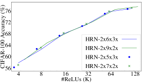
(a) DeepReDuce on CIFAR-100

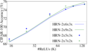
(b) SNL on CIFAR-100

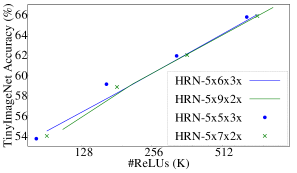
(c) DeepReDuce on TinyImageNet

Figure 21: Performance comparison of HRN networks designed for altered criticality order (Stage3 $>$ Stage4 $>$ Stage2 $>$ Stage1), HRNs with $\beta$=6 and 9, with the HRNs designed for prevalent criticality order (Stage3 $>$ Stage2 $>$ Stage4 $>$ Stage1), HRNs with $\beta$=5 and 7. Overall, the latter exhibit a slightly better performance than the former.

Appendix G Experimental Results and Discussion for ReLU-reuse

G.1 Ablation Study on ResNet18

We conducted an ablation study on ResNet18 (CIFAR-100) to investigate the benefits of two techniques: (1) using a shortcut connection between the output of one feature-subspace and the input of the next feature-subspace (shown in Figure 9), and (2) utilizing a fixed number of divisions, independent of the ReLU reduction factor. To evaluate the impact of these techniques, we applied ReLU-reuse on alternate convolution layers of ResNet18 and measured the resulting accuracy, which is reported in Table 14. Our findings suggest shortcut connections (i.e., with Reuse) improve accuracy, particularly at lower ReLU reduction factors. However, as the ReLU reduction factor increases, the accuracy gain diminishes. For instance, both with and without shortcut connections, we observed a drop of $\approx$1.5% in accuracy when moving from 2$\times$ to 4$\times$ reduction.

Table 14: We conduct an ablation analysis for ReLU-reuse by integrating it into alternating convolutional layers in ResNet18(CIFAR-100 dataset). For $N$ partitions, “reuse" signifies a shortcut connection between the output of one feature-subspace and the input of the subsequent one. In our proposed ReLU-reuse, the number of divisions remains constant regardless of the ReLU reduction factor, offering scalability for greater ReLU reduction factors.

ReLU reduction factor	ReLU count	$N$ divisions		Proposed
		w/o Reuse	w/ Reuse	($3$ divisions)
2x reduction (Scale=2)	434.18K	77.61%	78.19%	77.83%
4x reduction (Scale=4)	372.74K	75.84%	76.87%	77.60%
8x reduction (Scale=8)	342.02K	75.43%	75.66%	76.93%
16x reduction (Scale=16)	326.66K	75.33%	75.47%	76.38%

On the other hand, when using a fixed number of divisions in the proposed ReLU-reuse, accuracy drops remain (relatively) stable at higher reduction factors, underscoring the significance of a fixed number of divisions and also highlight their scalability for achieving higher ReLU reduction. Nonetheless, the proposed ReLU-reuse technique has lower accuracy at scale=2 than the $N$ division with shortcut connections. This is because the latter consists of only two groups of feature maps, while the former has three, which resulted in more information loss.

G.2 Performance Comparison of HRN vs. Classical Networks for ReLU-reuse

We compare ReLU-reuse against the conventional scaling method (channel/feature-map scaling) used in DeepReduce Jha et al. (2021) on both classical networks and HRNs. To begin with, we employ ReLU-reuse to all the convolutional layers of the networks and reduce the ReLUs by a factor of $N$ $\in$ {2, 4, 8, 16}. For $N=2$, we use the naive ReLU reduction method, as it outperforms the proposed ReLU-reuse (see Figure 9). Our findings reveal that for ResNet18 BaseCh networks, the performance of ReLU-reuse is suboptimal compared to conventional scaling methods, and this performance gap increases for the networks with higher $m$. In contrast, on the HRN networks, ReLU-reuse surpasses conventional scaling at higher ReLU reduction factors (at very low ReLU counts). However, at higher ReLUs, particularly for the ReLU reduction factor of two, the information loss resulting from the division of feature maps outweighs the ReLU-reuse benefits, leading to inferior ReLU-reuse performance. We emphasize that this observation holds even for networks with partial ReLU-equalization, such as ResNet18($m$=16)-4x4x4x.

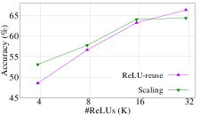
(a) ResNet18($m$=16)

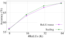
(b) ResNet18($m$=32)

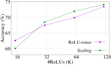
(c) ResNet18($m$=64)

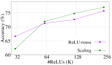
(d) ResNet18($m$=128)

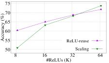
(e) 4x4x4x

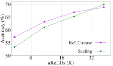
(f) HRN-2x6x2x

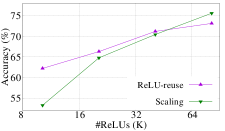
(g) HRN-5x5x3x

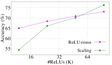
(h) HRN-6x6x2x

Figure 23: Performance comparison (CIFAR-100) of ReLU-reuse vs conventional scaling (used as reshaping steps in DeepReDuce Jha et al. (2021)) when ReLU-reuse is employed in Thinned networks. That is, first ReLU is dropped from every-alternate layers, and then ReLU-reuse is applied in remaining layers.

Furthermore, we conduct the same experiments on Thinned networks, as (channel/feature-map) scaling is performed on Thinned networks in DeepReDuce Jha et al. (2021). We dropped ReLUs from alternate convolutional layers and applied ReLU-reuse in the remaining layers. The results are shown in Figure 23. Since ReLU-reuse is now only employed in half of the total number of layers, the cumulative information loss caused by the loss of cross-channel information in feature-map divisions is reduced. As a result, the performance of ReLU-reuse is further enhanced. This improvement is evident from the change in the performance gap between ReLU-reuse and conventional scaling for all the networks, as shown in Figure 23.

To summarize, the effectiveness of ReLU-reuse depends on the network architecture and the ReLU reduction factor used. Specifically, ReLU-reuse is effective for the networks with (partial/full) ReLU equalization, in contrast with the classical networks, and scales well with higher ReLU reduction factors. Conclusively, ReLU-Thinned HRN networks combined with ReLU-reuse significantly improve the performance at very low ReLU counts, and should be further explored in future research.

Algorithm 2 ReLU optimization steps employed in HybReNets(HRNs)

Input: A network $Net$ with $D$ stages $S_{1}$, $S_{2}$, …, $S_{D}$ and $C$, a sorted list of stages from least to most critical
Output: ReLU optimized versions of $Net$

1:if the least critical stage C[1] dominates the distribution of ReLUs then

2:     $S_{k}$ = $C[1]$ $\triangleright$ Get the least critical stage

3:     $Net$ = $Net$ - $S_{k}$ $\triangleright$ Cull the least critical Stage $S_{k}$

4:end if

5:$Net_{i}^{T}$ = Thin($Net$) $\triangleright$ Thin the remaining stages

6:$Net_{i}^{C}$ = ScaleCh($Net_{i}^{T}$, $\alpha$=0.5) $\triangleright$ Channel scaled by 0.5x

7:$Net_{i}^{R4}$ = ReuseReLU ($Net_{i}^{T}$, Sc=4) $\triangleright$ ReLU-reuse with scaling factor 4

8:$Net_{i}^{R8}$ = ReuseReLU ($Net_{i}^{T}$, Sc=8) $\triangleright$ ReLU-reuse with scaling factor 8

9:$Net_{i}^{R16}$ = ReuseReLU ($Net_{i}^{T}$, Sc=16) $\triangleright$ ReLU-reuse with scaling factor 16

10:$Nets$ += $Net$, $Net_{i}^{T}$, $Net_{i}^{C}$, $Net_{i}^{R4}$, $Net_{i}^{R8}$, $Net_{i}^{R16}$ $\triangleright$ Apply KD to each Net

11:return $Nets$

Appendix H Design of Experiments and Training Procedure

Sweeping the width hyperparameters for ReLU efficiency experiments: For the network width-based experiments conducted on ResNet models, as illustrated in Figure 3 (a,b), we reduced the base channel count in ResNet18 to $m$=16 (from $m$=64). This adjustment is required to enable a fair comparison for ResNet models, as the vanilla ResNet20, ResNet32, and ResNet56 have {16, 32, 64} #channels in their successive stages while that in (original) ResNet18 is {64, 128, 256, 512}. For BaseCh networks, we sweep $m\in${16,32,64,128,256} and for StageCh networks, we sweep ($\alpha$, $\beta$, $\gamma$) = (2, 2, 2) to (8, 8, 8), homogeneously.

Training methodology and datasets: We perform our experiments on CIFAR-100 Krizhevsky et al. (2010) and TinyImageNet Le & Yang (2015); Yao & Miller (2015) as the prior PI-specific network optimization Jha et al. (2021); Cho et al. (2022b); Kundu et al. (2023a) used these datasets to evaluate their techniques. CIFAR-100 has 100 output classes, each having 500 training and 100 test images of resolution 32$\times$32. TinyImageNet, on the other hand, has 200 output classes, each containing 500 training and 50 validation images, each of resolution 64$\times$64.

In training, on both the CIFAR-100 and TinyImageNet datasets, we use cosine annealing learning rate scheduler Loshchilov & Hutter (2016) with an initial learning rate of $0.1$, mini-batch size of 128, momentum of $0.9$, and $0.0004$ weight decay factor. We train networks for 200 epochs on CIFAR-100 and TinyImageNet; however, we perform 20 additional epochs for warmup using Decoupled KD (Zhao et al., 2022). For DeepReDuce experiments and KD experiments in Tables 5, 11, and 12, we employ Hinton’s knowledge distillation Hinton et al. (2015) and set the temperature, and relative weight to cross-entropy loss on challenging targets as $4$ and $0.9$, respectively. For SNL, we train the baseline networks using the aforementioned methodology; however, we used their default implementation for mask generation, fine-tuning, and knowledge distillation. When employing Decoupled knowledge distillation (Tables 5, 11, and 12), we set the relative weight of target class KD as one and vary the weight of non-target class KD as {0.8, 1, 2, 6}. For every experiment involving knowledge distillation, we consistently employed ResNet18 as the teacher model for a fair comparison across the studies.

Runtime measurement: We adopt the methodology described in Garimella et al. (2023) for computing the runtime of a single (private) inference. In particular, we use Microsoft-SEAL for computing the homomorphic encryption (HE) latency, stemming from convolution and fully-connected operations, and DELPHI Mishra et al. (2020) implementation of Garbled-circuit for computing the garbled-circuit (GC) latency, stemming from ReLU operators. Our experimental setup involves an AMD EPYC 7502 server with specifications of 2.5 GHz, 32 cores, and 256 GB RAM. The client and server are simulated for these experiments as two separate processes operating on the same machine. We set the number of threads to four to compute the GC latency. Note that, for HRNs with ReLU-reuse, we calculated the HE latency without accounting for the FLOP reduction, stemming from the group convolution in ReLU-reuse due to specific implementation constraints of group convolution in Microsoft SEAL.

Appendix I Network Architecture of HybReNets

Table 15 provides a side-by-side comparison of design hyper-parameters between conventional models like WideResNet and ResNet and the ReLU efficient baseline network, CryptoNAS. This is contrasted against our newly proposed HybReNets. Table 16 contrasts ResNet18 and WRN22x8 with four specific HRNs: HRN-5x5x3x, HRN-5x7x2x, HRN-6x6x2x, and HRN-7x5x2x. Notably, in comparison to ResNet18, the HRNs allocate fewer channels during the initial phases and increase them in the deeper phases. This results in a more balanced ReLU-FLOP-Accuracy tradeoffs. We observed that HRN-5x5x3x offers a slightly better ReLU-FLOP-Accuracy benefits than other HRNs.

Table 17 details the architectural specifics of HRNs when $\alpha$=2, which are crucial for performing PI at lower ReLU counts. It is important to point out that these HRNs build upon the ResNet18 architecture, leading to their stages computing ratios of [2, 2, 2, 2]. In a similar vein, HRNs based on other baseline networks like ResNet34 will have stage-compute ratios aligning with ResNet34, which are [3, 4, 6, 3].

Table 15: Comparison of channel scaling techniques in different network architectures. WideResNets use uniform scaling with every layer scaled by a factor of $k$. CryptoNAS Ghodsi et al. (2020), a family of ReLU efficient baseline networks, scale homogeneously, increasing channels in subsequent stages by a factor of 4. HybReNet (proposed), on the other hand, applies heterogeneous scaling: Stage2 by $\alpha$, Stage3 by $\beta$, and Stage4 by $\gamma$, aiming to optimize both ReLU and FLOP efficiency.

Stages	output size	ResNet	WideResNet	CryptoNAS	HybReNet(Proposed)
Stem	$d_{in}\times d_{in}$	[3$\times$3, $m$]	[3$\times$3, $m$]	[3$\times$3, $m$]	[3$\times$3, $m$]
Stage1	$d_{in}$$\times$$d_{in}$	$\left[\begin{array}[]{c}\text{3$\times$3, $m$}\\[-1.00006pt] \text{3$\times$3, $m$}\end{array}\right]$$\times$$\phi_{1}$	$\left[\begin{array}[]{c}\text{3$\times$3, $m$$\times$k}\\[-1.00006pt] \text{3$\times$3, $m$$\times$k}\end{array}\right]$$\times$$\phi_{1}$	$\left[\begin{array}[]{c}\text{3$\times$3, $m$}\\[-1.00006pt] \text{3$\times$3, $m$}\end{array}\right]$$\times$$\phi_{1}$	$\left[\begin{array}[]{c}\text{3$\times$3, $m$}\\[-1.00006pt] \text{3$\times$3, $m$}\end{array}\right]$$\times$$\phi_{1}$
Stage2	$\frac{d_{in}}{2}$$\times$$\frac{d_{in}}{2}$	$\left[\begin{array}[]{c}\text{3$\times$3, $2m$}\\[-1.00006pt] \text{3$\times$3, $2m$}\end{array}\right]$$\times$$\phi_{2}$	$\left[\begin{array}[]{c}\text{3$\times$3, $2m$$\times$k}\\[-1.00006pt] \text{3$\times$3, $2m$$\times$k}\end{array}\right]$$\times$$\phi_{2}$	$\left[\begin{array}[]{c}\text{3$\times$3, $4m$}\\[-1.00006pt] \text{3$\times$3, $4m$}\end{array}\right]$$\times$$\phi_{2}$	$\left[\begin{array}[]{c}\text{3$\times$3, $\alpha m$}\\[-1.00006pt] \text{3$\times$3, $\alpha m$}\end{array}\right]$$\times$$\phi_{2}$
Stage3	$\frac{d_{in}}{4}$$\times$$\frac{d_{in}}{4}$	$\left[\begin{array}[]{c}\text{3$\times$3, $4m$}\\[-1.00006pt] \text{3$\times$3, $4m$}\end{array}\right]$$\times$$\phi_{3}$	$\left[\begin{array}[]{c}\text{3$\times$3, $4m$$\times$k}\\[-1.00006pt] \text{3$\times$3, $4m$$\times$k}\end{array}\right]$$\times$$\phi_{3}$	$\left[\begin{array}[]{c}\text{3$\times$3, $16m$}\\[-1.00006pt] \text{3$\times$3, $16m$}\end{array}\right]$$\times$$\phi_{3}$	$\left[\begin{array}[]{c}\text{3$\times$3, $\beta(\alpha m)$}\\[-1.00006pt] \text{3$\times$3, $\beta(\alpha m)$}\end{array}\right]$$\times$$\phi_{3}$
Stage4	$\frac{d_{in}}{8}$$\times$$\frac{d_{in}}{8}$	$\left[\begin{array}[]{c}\text{3$\times$3, $8m$}\\[-1.00006pt] \text{3$\times$3, $8m$}\end{array}\right]$$\times$$\phi_{4}$			$\left[\begin{array}[]{c}\text{3$\times$3, $\gamma(\alpha\beta m)$}\\[-1.00006pt] \text{3$\times$3, $\gamma(\alpha\beta m)$}\end{array}\right]$$\times$$\phi_{4}$
FC	$1\times 1$	[$\frac{d_{in}}{8}\times\frac{d_{in}}{8}$, $8m$]	[$\frac{d_{in}}{4}\times\frac{d_{in}}{4}$, $4m\times k$]	[$\frac{d_{in}}{4}\times\frac{d_{in}}{4}$, $16m$]	[$\frac{d_{in}}{8}\times\frac{d_{in}}{8}$, $\gamma(\alpha\beta m)$]

• WideResNet and CryptoNAS differ from ResNet in their skip-connection styles, the positioning of ReLU layers (pre-activation or post-activation).

Table 16: Comparison of WideResNet22x8 and ResNet18 architecture — predominantly used as input baseline networks in PI-specific ReLU optimization techniques Kundu et al. (2023a); Cho et al. (2022b); Jha et al. (2021) — with our proposed HybReNets (highlighted in bold). Unlike the conventional WideResNets and ResNets, the strategic channel allocation in subsequent stages of HybReNets streamline the network’s ReLUs and FLOPs, and simultaneously optimized both the ReLU and FLOPs efficiency. Last rows compare their FLOPs and ReLU counts, along with baseline accuracy (on CIFAR-100).

Stages	output size	WRN22x8	ResNet18	HRN-5x5x3x	HRN-5x7x2x	HRN-6x6x2x	HRN-7x5x2x
Stem	$32\times 32$	[3$\times$3, $16$]	[3$\times$3, $64$]	[3$\times$3, $16$]	[3$\times$3, $16$]	[3$\times$3, $16$]	[3$\times$3, $16$]
Stage1	$32$$\times$$32$	$\left[\begin{array}[]{c}\text{3$\times$3, $128$}\\[-1.00006pt] \text{3$\times$3, $128$}\end{array}\right]$$\times$$3$	$\left[\begin{array}[]{c}\text{3$\times$3, $64$}\\[-1.00006pt] \text{3$\times$3, $64$}\end{array}\right]$$\times$$2$	$\left[\begin{array}[]{c}\text{3$\times$3, $16$}\\[-1.00006pt] \text{3$\times$3, $16$}\end{array}\right]$$\times$$2$	$\left[\begin{array}[]{c}\text{3$\times$3, $16$}\\[-1.00006pt] \text{3$\times$3, $16$}\end{array}\right]$$\times$$2$	$\left[\begin{array}[]{c}\text{3$\times$3, $16$}\\[-1.00006pt] \text{3$\times$3, $16$}\end{array}\right]$$\times$$2$	$\left[\begin{array}[]{c}\text{3$\times$3, $16$}\\[-1.00006pt] \text{3$\times$3, $16$}\end{array}\right]$$\times$$2$
Stage2	$16$$\times$$16$	$\left[\begin{array}[]{c}\text{3$\times$3, $256$}\\[-1.00006pt] \text{3$\times$3, $256$}\end{array}\right]$$\times$$3$	$\left[\begin{array}[]{c}\text{3$\times$3, $128$}\\[-1.00006pt] \text{3$\times$3, $128$}\end{array}\right]$$\times$$2$	$\left[\begin{array}[]{c}\text{3$\times$3, $80$}\\[-1.00006pt] \text{3$\times$3, $80$}\end{array}\right]$$\times$$2$	$\left[\begin{array}[]{c}\text{3$\times$3, $80$}\\[-1.00006pt] \text{3$\times$3, $80$}\end{array}\right]$$\times$$2$	$\left[\begin{array}[]{c}\text{3$\times$3, $96$}\\[-1.00006pt] \text{3$\times$3, $96$}\end{array}\right]$$\times$$2$	$\left[\begin{array}[]{c}\text{3$\times$3, $112$}\\[-1.00006pt] \text{3$\times$3, $112$}\end{array}\right]$$\times$$2$
Stage3	$8$$\times$$8$	$\left[\begin{array}[]{c}\text{3$\times$3, $512$}\\[-1.00006pt] \text{3$\times$3, $512$}\end{array}\right]$$\times$$3$	$\left[\begin{array}[]{c}\text{3$\times$3, $256$}\\[-1.00006pt] \text{3$\times$3, $256$}\end{array}\right]$$\times$$2$	$\left[\begin{array}[]{c}\text{3$\times$3, $400$}\\[-1.00006pt] \text{3$\times$3, $400$}\end{array}\right]$$\times$$2$	$\left[\begin{array}[]{c}\text{3$\times$3, $560$}\\[-1.00006pt] \text{3$\times$3, $560$}\end{array}\right]$$\times$$2$	$\left[\begin{array}[]{c}\text{3$\times$3, $576$}\\[-1.00006pt] \text{3$\times$3, $576$}\end{array}\right]$$\times$$2$	$\left[\begin{array}[]{c}\text{3$\times$3, $560$}\\[-1.00006pt] \text{3$\times$3, $560$}\end{array}\right]$$\times$$2$
Stage4	$4$$\times$$4$		$\left[\begin{array}[]{c}\text{3$\times$3, $512$}\\[-1.00006pt] \text{3$\times$3, $512$}\end{array}\right]$$\times$$2$	$\left[\begin{array}[]{c}\text{3$\times$3, $1200$}\\[-1.00006pt] \text{3$\times$3, $1200$}\end{array}\right]$$\times$$2$	$\left[\begin{array}[]{c}\text{3$\times$3, $1120$}\\[-1.00006pt] \text{3$\times$3, $1120$}\end{array}\right]$$\times$$2$	$\left[\begin{array}[]{c}\text{3$\times$3, $1152$}\\[-1.00006pt] \text{3$\times$3, $1152$}\end{array}\right]$$\times$$2$	$\left[\begin{array}[]{c}\text{3$\times$3, $1120$}\\[-1.00006pt] \text{3$\times$3, $1120$}\end{array}\right]$$\times$$2$
FC	$1\times 1$	[$8\times 8$, $512$]	[$4\times 4$, $512$]	[$4\times 4$, $1200$]	[$4\times 4$, $1120$]	[$4\times 4$, $1152$]	[$4\times 4$, $1120$]
#FLOPs		2461M	559M	1055M	1273M	1368M	1328M
#ReLUs		1393K	557K	343K	379K	401K	412K
Accuracy		81.27%	79.01%	78.40%	78.28%	78.52%	78.81%

Table 17: Baseline HybReNets (built on ResNet18 architecture) aim for efficient PI with lower ReLU counts. The final rows show a comparison of their FLOPs, ReLU counts, and baseline accuracy on CIFAR-100 dataset.

Stages	output size	HRN-2x5x3x	HRN-2x7x2x	HRN-2x6x2x	HRN-2x5x2x
Stem	$32\times 32$	[3$\times$3, $16$]	[3$\times$3, $16$]	[3$\times$3, $16$]	[3$\times$3, $16$]
Stage1	$32$$\times$$32$	$\left[\begin{array}[]{c}\text{3$\times$3, $16$}\\[-1.00006pt] \text{3$\times$3, $16$}\end{array}\right]$$\times$$2$	$\left[\begin{array}[]{c}\text{3$\times$3, $16$}\\[-1.00006pt] \text{3$\times$3, $16$}\end{array}\right]$$\times$$2$	$\left[\begin{array}[]{c}\text{3$\times$3, $16$}\\[-1.00006pt] \text{3$\times$3, $16$}\end{array}\right]$$\times$$2$	$\left[\begin{array}[]{c}\text{3$\times$3, $16$}\\[-1.00006pt] \text{3$\times$3, $16$}\end{array}\right]$$\times$$2$
Stage2	$16$$\times$$16$	$\left[\begin{array}[]{c}\text{3$\times$3, $32$}\\[-1.00006pt] \text{3$\times$3, $32$}\end{array}\right]$$\times$$2$	$\left[\begin{array}[]{c}\text{3$\times$3, $32$}\\[-1.00006pt] \text{3$\times$3, $32$}\end{array}\right]$$\times$$2$	$\left[\begin{array}[]{c}\text{3$\times$3, $32$}\\[-1.00006pt] \text{3$\times$3, $32$}\end{array}\right]$$\times$$2$	$\left[\begin{array}[]{c}\text{3$\times$3, $32$}\\[-1.00006pt] \text{3$\times$3, $32$}\end{array}\right]$$\times$$2$
Stage3	$8$$\times$$8$	$\left[\begin{array}[]{c}\text{3$\times$3, $160$}\\[-1.00006pt] \text{3$\times$3, $160$}\end{array}\right]$$\times$$2$	$\left[\begin{array}[]{c}\text{3$\times$3, $224$}\\[-1.00006pt] \text{3$\times$3, $224$}\end{array}\right]$$\times$$2$	$\left[\begin{array}[]{c}\text{3$\times$3, $192$}\\[-1.00006pt] \text{3$\times$3, $192$}\end{array}\right]$$\times$$2$	$\left[\begin{array}[]{c}\text{3$\times$3, $160$}\\[-1.00006pt] \text{3$\times$3, $160$}\end{array}\right]$$\times$$2$
Stage4	$4$$\times$$4$	$\left[\begin{array}[]{c}\text{3$\times$3, $480$}\\[-1.00006pt] \text{3$\times$3, $480$}\end{array}\right]$$\times$$2$	$\left[\begin{array}[]{c}\text{3$\times$3, $448$}\\[-1.00006pt] \text{3$\times$3, $448$}\end{array}\right]$$\times$$2$	$\left[\begin{array}[]{c}\text{3$\times$3, $384$}\\[-1.00006pt] \text{3$\times$3, $384$}\end{array}\right]$$\times$$2$	$\left[\begin{array}[]{c}\text{3$\times$3, $320$}\\[-1.00006pt] \text{3$\times$3, $320$}\end{array}\right]$$\times$$2$
FC	$1\times 1$	[$8\times 8$, $480$]	[$4\times 4$, $448$]	[$4\times 4$, $384$]	[$4\times 4$, $320$]
#FLOPs		179M	213M	163M	119M
#ReLUs		186K	201K	188K	176K
Accuracy		75.34%	75.73%	75.70%	75.03%

References

- Aharoni et al. (2023) Ehud Aharoni, Allon Adir, Moran Baruch, Nir Drucker, Gilad Ezov, Ariel Farkash, Lev Greenberg, Ramy Masalha, Guy Moshkowich, Dov Murik, et al. Helayers: A tile tensors framework for large neural networks on encrypted data. Proceedings on privacy enhancing technologies, 2023.
- Akimoto et al. (2023) Yoshimasa Akimoto, Kazuto Fukuchi, Youhei Akimoto, and Jun Sakuma. Privformer: Privacy-preserving transformer with mpc. In IEEE 8th European Symposium on Security and Privacy (EuroS&P), 2023.
- Ali et al. (2020) Ramy E Ali, Jinhyun So, and A Salman Avestimehr. On polynomial approximations for privacy-preserving and verifiable relu networks. arXiv preprint arXiv:2011.05530, 2020.
- Ball et al. (2019) Marshall Ball, Brent Carmer, Tal Malkin, Mike Rosulek, and Nichole Schimanski. Garbled neural networks are practical. Cryptology ePrint Archive, 2019.
- Balunović & Vechev (2020) Mislav Balunović and Martin Vechev. Adversarial training and provable defenses: Bridging the gap. In International Conference on Learning Representations, 2020.
- Belkin et al. (2019) Mikhail Belkin, Daniel Hsu, Siyuan Ma, and Soumik Mandal. Reconciling modern machine-learning practice and the classical bias–variance trade-off. Proceedings of the National Academy of Sciences, 2019.
- Brakerski et al. (2014) Zvika Brakerski, Craig Gentry, and Vinod Vaikuntanathan. (leveled) fully homomorphic encryption without bootstrapping. ACM Transactions on Computation Theory, 2014.
- Chang et al. (2018) Julie Chang, Vincent Sitzmann, Xiong Dun, Wolfgang Heidrich, and Gordon Wetzstein. Hybrid optical-electronic convolutional neural networks with optimized diffractive optics for image classification. Scientific reports, 2018.
- Chen et al. (2022a) Tianlong Chen, Huan Zhang, Zhenyu Zhang, Shiyu Chang, Sijia Liu, Pin-Yu Chen, and Zhangyang Wang. Linearity grafting: Relaxed neuron pruning helps certifiable robustness. In International Conference on Machine Learning, 2022a.
- Chen et al. (2022b) Tianyu Chen, Hangbo Bao, Shaohan Huang, Li Dong, Binxing Jiao, Daxin Jiang, Haoyi Zhou, Jianxin Li, and Furu Wei. THE-X: Privacy-preserving transformer inference with homomorphic encryption. In Findings of the Association for Computational Linguistics(ACL), 2022b.
- Cheon et al. (2017) Jung Hee Cheon, Andrey Kim, Miran Kim, and Yongsoo Song. Homomorphic encryption for arithmetic of approximate numbers. In International conference on the theory and application of cryptology and information security, 2017.
- Cho et al. (2022a) Minsu Cho, Zahra Ghodsi, Brandon Reagen, Siddharth Garg, and Chinmay Hegde. Sphynx: Relu-efficient network design for private inference. IEEE Security & Privacy, 2022a.
- Cho et al. (2022b) Minsu Cho, Ameya Joshi, Siddharth Garg, Brandon Reagen, and Chinmay Hegde. Selective network linearization for efficient private inference. In International Conference on Machine Learning, 2022b.
- Cohen & Welling (2017) Taco S. Cohen and Max Welling. Steerable CNNs. In International Conference on Learning Representations, 2017.
- Demmler et al. (2015) Daniel Demmler, Thomas Schneider, and Michael Zohner. Aby-a framework for efficient mixed-protocol secure two-party computation. In The Network and Distributed System Security Symposium, 2015.
- Dollár et al. (2021) Piotr Dollár, Mannat Singh, and Ross Girshick. Fast and accurate model scaling. In Proceedings of the IEEE/CVF Conference on Computer Vision and Pattern Recognition, 2021.
- Dror et al. (2021) Amir Ben Dror, Niv Zehngut, Avraham Raviv, Evgeny Artyomov, Ran Vitek, and Roy Josef Jevnisek. Layer folding: Neural network depth reduction using activation linearization. In British Machine Vision Conference, 2021.
- Eisenhofer et al. (2022) Thorsten Eisenhofer, Doreen Riepel, Varun Chandrasekaran, Esha Ghosh, Olga Ohrimenko, and Nicolas Papernot. Verifiable and provably secure machine unlearning. arXiv preprint arXiv:2210.09126, 2022.
- Fan & Vercauteren (2012) Junfeng Fan and Frederik Vercauteren. Somewhat practical fully homomorphic encryption. Cryptology ePrint Archive, 2012.
- Fan et al. (2022) Xiaoyu Fan, Kun Chen, Guosai Wang, Mingchun Zhuang, Yi Li, and Wei Xu. Nfgen: Automatic non-linear function evaluation code generator for general-purpose mpc platforms. In Proceedings of the 2022 ACM SIGSAC Conference on Computer and Communications Security, 2022.
- Franzen & Wand (2021) Daniel Franzen and Michael Wand. General nonlinearities in so(2)-equivariant cnns. In Advances in Neural Information Processing Systems, 2021.
- Gao et al. (2019) Shanghua Gao, Ming-Ming Cheng, Kai Zhao, Xin-Yu Zhang, Ming-Hsuan Yang, and Philip HS Torr. Res2net: A new multi-scale backbone architecture. In IEEE transactions on pattern analysis and machine intelligence, 2019.
- Garimella et al. (2021) Karthik Garimella, Nandan Kumar Jha, and Brandon Reagen. Sisyphus: A cautionary tale of using low-degree polynomial activations in privacy-preserving deep learning. In ACM CCS Workshop on Private-preserving Machine Learning, 2021.
- Garimella et al. (2023) Karthik Garimella, Zahra Ghodsi, Nandan Kumar Jha, Siddharth Garg, and Brandon Reagen. Characterizing and optimizing end-to-end systems for private inference. In Proceedings of the 28th ACM International Conference on Architectural Support for Programming Languages and Operating Systems, 2023.
- Gentry et al. (2009) Craig Gentry et al. A fully homomorphic encryption scheme. 2009.
- Ghodsi et al. (2020) Zahra Ghodsi, Akshaj Kumar Veldanda, Brandon Reagen, and Siddharth Garg. CryptoNAS: Private inference on a relu budget. In Advances in Neural Information Processing Systems, 2020.
- Ghodsi et al. (2021) Zahra Ghodsi, Nandan Kumar Jha, Brandon Reagen, and Siddharth Garg. Circa: Stochastic relus for private deep learning. In Advances in Neural Information Processing Systems, 2021.
- Golubeva et al. (2021) Anna Golubeva, Guy Gur-Ari, and Behnam Neyshabur. Are wider nets better given the same number of parameters? In International Conference on Learning Representations, 2021.
- Gupta et al. (2023) Kanav Gupta, Neha Jawalkar, Ananta Mukherjee, Nishanth Chandran, Divya Gupta, Ashish Panwar, and Rahul Sharma. Sigma: Secure gpt inference with function secret sharing. Cryptology ePrint Archive, 2023.
- Gupta et al. (2022) Udit Gupta, Mariam Elgamal, Gage Hills, Gu-Yeon Wei, Hsien-Hsin S Lee, David Brooks, and Carole-Jean Wu. Act: Designing sustainable computer systems with an architectural carbon modeling tool. In Proceedings of the 49th Annual International Symposium on Computer Architecture, pp. 784–799, 2022.
- Hao et al. (2022) Meng Hao, Hongwei Li, Hanxiao Chen, Pengzhi Xing, Guowen Xu, and Tianwei Zhang. Iron: Private inference on transformers. In Advances in Neural Information Processing Systems, 2022.
- He et al. (2016) Kaiming He, Xiangyu Zhang, Shaoqing Ren, and Jian Sun. Deep residual learning for image recognition. In Proceedings of the IEEE conference on computer vision and pattern recognition, 2016.
- Hinton et al. (2015) Geoffrey Hinton, Oriol Vinyals, and Jeff Dean. Distilling the knowledge in a neural network. arXiv preprint arXiv:1503.02531, 2015.
- Hou et al. (2023) Xiaoyang Hou, Jian Liu, Jingyu Li, Yuhan Li, Wen-jie Lu, Cheng Hong, and Kui Ren. Ciphergpt: Secure two-party gpt inference. Cryptology ePrint Archive, 2023.
- Howard et al. (2019) Andrew Howard, Mark Sandler, Grace Chu, Liang-Chieh Chen, Bo Chen, Mingxing Tan, Weijun Wang, Yukun Zhu, Ruoming Pang, Vijay Vasudevan, et al. Searching for mobilenetv3. In Proceedings of the IEEE/CVF International Conference on Computer Vision, 2019.
- Howard et al. (2017) Andrew G Howard, Menglong Zhu, Bo Chen, Dmitry Kalenichenko, Weijun Wang, Tobias Weyand, Marco Andreetto, and Hartwig Adam. Mobilenets: Efficient convolutional neural networks for mobile vision applications. arXiv preprint, 2017.
- Huang et al. (2022) Zhicong Huang, Wen jie Lu, Cheng Hong, and Jiansheng Ding. Cheetah: Lean and fast secure Two-Party deep neural network inference. In 31st USENIX Security Symposium, 2022.
- Jha et al. (2021) Nandan Kumar Jha, Zahra Ghodsi, Siddharth Garg, and Brandon Reagen. DeepReDuce: Relu reduction for fast private inference. In International Conference on Machine Learning, 2021.
- Juvekar et al. (2018) Chiraag Juvekar, Vinod Vaikuntanathan, and Anantha Chandrakasan. Gazelle: A low latency framework for secure neural network inference. In 27th USENIX Security Symposium, 2018.
- Kang et al. (2022) Daniel Kang, Tatsunori Hashimoto, Ion Stoica, and Yi Sun. Scaling up trustless dnn inference with zero-knowledge proofs. arXiv preprint arXiv:2210.08674, 2022.
- Knott et al. (2021) Brian Knott, Shobha Venkataraman, Awni Hannun, Shubho Sengupta, Mark Ibrahim, and Laurens van der Maaten. Crypten: Secure multi-party computation meets machine learning. Advances in Neural Information Processing Systems, 2021.
- Krizhevsky et al. (2010) Alex Krizhevsky, Vinod Nair, and Geoffrey Hinton. Cifar-10 (canadian institute for advanced research). URL http://www. cs. toronto. edu/kriz/cifar. html, 2010.
- Kundu et al. (2023a) Souvik Kundu, Shunlin Lu, Yuke Zhang, Jacqueline Liu, and Peter A Beerel. Learning to linearize deep neural networks for secure and efficient private inference. In The Eleventh International Conference on Learning Representations, 2023a.
- Kundu et al. (2023b) Souvik Kundu, Yuke Zhang, Dake Chen, and Peter A. Beerel. Making models shallow again: Jointly learning to reduce non-linearity and depth for latency-efficient private inference. In Proceedings of the IEEE/CVF Conference on Computer Vision and Pattern Recognition (CVPR) Workshops, 2023b.
- Le & Yang (2015) Ya Le and Xuan Yang. Tiny imagenet visual recognition challenge. CS 231N, 7, 2015.
- Lee et al. (2022) Eunsang Lee, Joon-Woo Lee, Junghyun Lee, Young-Sik Kim, Yongjune Kim, Jong-Seon No, and Woosuk Choi. Low-complexity deep convolutional neural networks on fully homomorphic encryption using multiplexed parallel convolutions. In International Conference on Machine Learning, 2022.
- Lee et al. (2019) Jaehoon Lee, Lechao Xiao, Samuel Schoenholz, Yasaman Bahri, Roman Novak, Jascha Sohl-Dickstein, and Jeffrey Pennington. Wide neural networks of any depth evolve as linear models under gradient descent. Advances in neural information processing systems, 32, 2019.
- Li et al. (2023) Dacheng Li, Hongyi Wang, Rulin Shao, Han Guo, Eric Xing, and Hao Zhang. MPCFORMER: FAST, PERFORMANT AND PRIVATE TRANSFORMER INFERENCE WITH MPC. In The Eleventh International Conference on Learning Representations, 2023.
- Li et al. (2022) Gordon HY Li, Ryoto Sekine, Rajveer Nehra, Robert M Gray, Luis Ledezma, Qiushi Guo, and Alireza Marandi. All-optical ultrafast relu function for energy-efficient nanophotonic deep learning. Nanophotonics, 2022.
- Li et al. (2018) Hao Li, Zheng Xu, Gavin Taylor, Christoph Studer, and Tom Goldstein. Visualizing the loss landscape of neural nets. Advances in neural information processing systems, 2018.
- Liu et al. (2018) Hanxiao Liu, Karen Simonyan, and Yiming Yang. Darts: Differentiable architecture search. arXiv preprint, 2018.
- Liu et al. (2017) Jian Liu, Mika Juuti, Yao Lu, and N Asokan. Oblivious neural network predictions via minionn transformations. In Proceedings of the ACM SIGSAC Conference on Computer and Communications Security, 2017.
- Liu et al. (2021) Tianyi Liu, Xiang Xie, and Yupeng Zhang. Zkcnn: Zero knowledge proofs for convolutional neural network predictions and accuracy. In Proceedings of the 2021 ACM SIGSAC Conference on Computer and Communications Security, pp. 2968–2985, 2021.
- Liu et al. (2022) Zhuang Liu, Hanzi Mao, Chao-Yuan Wu, Christoph Feichtenhofer, Trevor Darrell, and Saining Xie. A convnet for the 2020s. In Proceedings of the IEEE/CVF Conference on Computer Vision and Pattern Recognition, 2022.
- Loshchilov & Hutter (2016) Ilya Loshchilov and Frank Hutter. Sgdr: Stochastic gradient descent with warm restarts. arXiv preprint arXiv:1608.03983, 2016.
- Lou et al. (2020a) Qian Lou, Song Bian, and Lei Jiang. Autoprivacy: Automated layer-wise parameter selection for secure neural network inference. In Advances in Neural Information Processing Systems, pp. 8638–8647, 2020a.
- Lou et al. (2020b) Qian Lou, Wen-jie Lu, Cheng Hong, and Lei Jiang. Falcon: fast spectral inference on encrypted data. Advances in Neural Information Processing Systems, 2020b.
- Lou et al. (2021) Qian Lou, Yilin Shen, Hongxia Jin, and Lei Jiang. SAFENet: Asecure, accurate and fast neu-ral network inference. International Conference on Learning Representations, 2021.
- Mirzadeh et al. (2022) Seyed Iman Mirzadeh, Arslan Chaudhry, Dong Yin, Huiyi Hu, Razvan Pascanu, Dilan Gorur, and Mehrdad Farajtabar. Wide neural networks forget less catastrophically. In International Conference on Machine Learning, 2022.
- Mishra et al. (2020) Pratyush Mishra, Ryan Lehmkuhl, Akshayaram Srinivasan, Wenting Zheng, and Raluca Ada Popa. Delphi: A cryptographic inference service for neural networks. In 29th USENIX Security Symposium, 2020.
- Mo et al. (2023) Jianqiao Mo, Jayanth Gopinath, and Brandon Reagen. Haac: A hardware-software co-design to accelerate garbled circuits. In Proceedings of the 50th Annual International Symposium on Computer Architecture, 2023.
- Mohassel & Rindal (2018) Payman Mohassel and Peter Rindal. Aby3: A mixed protocol framework for machine learning. In Proceedings of the ACM SIGSAC Conference on Computer and Communications Security, 2018.
- Nakkiran et al. (2021) Preetum Nakkiran, Gal Kaplun, Yamini Bansal, Tristan Yang, Boaz Barak, and Ilya Sutskever. Deep double descent: Where bigger models and more data hurt. Journal of Statistical Mechanics: Theory and Experiment, 2021.
- Ng & Chow (2023) Lucien KL Ng and Sherman SM Chow. Sok: Cryptographic neural-network computation. In 2023 IEEE Symposium on Security and Privacy (SP), 2023.
- Nguyen et al. (2021) Thao Nguyen, Maithra Raghu, and Simon Kornblith. Do wide and deep networks learn the same things? uncovering how neural network representations vary with width and depth. In International Conference on Learning Representations, 2021.
- Patra et al. (2021) Arpita Patra, Thomas Schneider, Ajith Suresh, and Hossein Yalame. Aby2.0: Improved mixed-protocol secure two-party computation. In 30th USENIX Security Symposium, 2021.
- Peng et al. (2023) Hongwu Peng, Shaoyi Huang, Tong Zhou, Yukui Luo, Chenghong Wang, Zigeng Wang, Jiahui Zhao, Xi Xie, Ang Li, Tony Geng, et al. Autorep: Automatic relu replacement for fast private network inference. In Proceedings of the IEEE/CVF International Conference on Computer Vision (ICCV), 2023.
- Radosavovic et al. (2019) Ilija Radosavovic, Justin Johnson, Saining Xie, Wan-Yen Lo, and Piotr Dollár. On network design spaces for visual recognition. In Proceedings of the IEEE/CVF international conference on computer vision, 2019.
- Radosavovic et al. (2020) Ilija Radosavovic, Raj Prateek Kosaraju, Ross Girshick, Kaiming He, and Piotr Dollár. Designing network design spaces. In Proceedings of the IEEE/CVF Conference on Computer Vision and Pattern Recognition, 2020.
- Rathee et al. (2020) Deevashwer Rathee, Mayank Rathee, Nishant Kumar, Nishanth Chandran, Divya Gupta, Aseem Rastogi, and Rahul Sharma. Cryptflow2: Practical 2-party secure inference. In Proceedings of the ACM SIGSAC Conference on Computer and Communications Security, 2020.
- Samardzic et al. (2021) Nikola Samardzic, Axel Feldmann, Aleksandar Krastev, Srinivas Devadas, Ronald Dreslinski, Christopher Peikert, and Daniel Sanchez. F1: A fast and programmable accelerator for fully homomorphic encryption. In 54th Annual IEEE/ACM International Symposium on Microarchitecture, 2021.
- Samardzic et al. (2022) Nikola Samardzic, Axel Feldmann, Aleksandar Krastev, Nathan Manohar, Nicholas Genise, Srinivas Devadas, Karim Eldefrawy, Chris Peikert, and Daniel Sanchez. Craterlake: a hardware accelerator for efficient unbounded computation on encrypted data. In ISCA, 2022.
- Sandler et al. (2018) Mark Sandler, Andrew Howard, Menglong Zhu, Andrey Zhmoginov, and Liang-Chieh Chen. Mobilenetv2: Inverted residuals and linear bottlenecks. In The IEEE Conference on Computer Vision and Pattern Recognition (CVPR), 2018.
- (74) SEAL. Microsoft SEAL (release 4.0). https://github.com/Microsoft/SEAL, March 2022. Microsoft Research, Redmond, WA.
- Shamir (1979) Adi Shamir. How to share a secret. Communications of the ACM, 1979.
- Somepalli et al. (2022) Gowthami Somepalli, Liam Fowl, Arpit Bansal, Ping Yeh-Chiang, Yehuda Dar, Richard Baraniuk, Micah Goldblum, and Tom Goldstein. Can neural nets learn the same model twice? investigating reproducibility and double descent from the decision boundary perspective. In Proceedings of the IEEE/CVF Conference on Computer Vision and Pattern Recognition, 2022.
- Sun & Zhang (2023) Haochen Sun and Hongyang Zhang. zkdl: Efficient zero-knowledge proofs of deep learning training. arXiv preprint arXiv:2307.16273, 2023.
- Szegedy et al. (2016) Christian Szegedy, Vincent Vanhoucke, Sergey Ioffe, Jon Shlens, and Zbigniew Wojna. Rethinking the inception architecture for computer vision. In Proceedings of the IEEE conference on computer vision and pattern recognition, 2016.
- Tan & Le (2019) Mingxing Tan and Quoc Le. Efficientnet: Rethinking model scaling for convolutional neural networks. In International Conference on Machine Learning, 2019.
- Tan & Le (2021) Mingxing Tan and Quoc Le. Efficientnetv2: Smaller models and faster training. In International conference on machine learning, 2021.
- Tan et al. (2019) Mingxing Tan, Bo Chen, Ruoming Pang, Vijay Vasudevan, Mark Sandler, Andrew Howard, and Quoc V Le. Mnasnet: Platform-aware neural architecture search for mobile. In Proceedings of the IEEE Conference on Computer Vision and Pattern Recognition, 2019.
- Tan et al. (2021) Sijun Tan, Brian Knott, Yuan Tian, and David J Wu. Cryptgpu: Fast privacy-preserving machine learning on the gpu. In IEEE Symposium on Security and Privacy, 2021.
- Wang et al. (2022) Yongqin Wang, G Edward Suh, Wenjie Xiong, Benjamin Lefaudeux, Brian Knott, Murali Annavaram, and Hsien-Hsin S Lee. Characterization of mpc-based private inference for transformer-based models. In IEEE International Symposium on Performance Analysis of Systems and Software (ISPASS), 2022.
- Weiler & Cesa (2019) Maurice Weiler and Gabriele Cesa. General e(2)-equivariant steerable cnns. Advances in Neural Information Processing Systems, 2019.
- Weiler et al. (2018) Maurice Weiler, Mario Geiger, Max Welling, Wouter Boomsma, and Taco S Cohen. 3d steerable cnns: Learning rotationally equivariant features in volumetric data. Advances in Neural Information Processing Systems, 2018.
- Woo et al. (2023) Sanghyun Woo, Shoubhik Debnath, Ronghang Hu, Xinlei Chen, Zhuang Liu, In So Kweon, and Saining Xie. Convnext v2: Co-designing and scaling convnets with masked autoencoders. In Proceedings of the IEEE/CVF Conference on Computer Vision and Pattern Recognition, 2023.
- Xiao et al. (2019) Kai Y. Xiao, Vincent Tjeng, Nur Muhammad (Mahi) Shafiullah, and Aleksander Madry. Training for faster adversarial robustness verification via inducing reLU stability. In International Conference on Learning Representations, 2019.
- Xie et al. (2017) Saining Xie, Ross Girshick, Piotr Dollár, Zhuowen Tu, and Kaiming He. Aggregated residual transformations for deep neural networks. In Proceedings of the IEEE conference on computer vision and pattern recognition, 2017.
- Yao (1986) Andrew Chi-Chih Yao. How to generate and exchange secrets. In 27th Annual Symposium on Foundations of Computer Science, 1986.
- Yao & Miller (2015) Leon Yao and John Miller. Tiny imagenet classification with convolutional neural networks. CS 231N, 2015.
- Yosinski et al. (2014) Jason Yosinski, Jeff Clune, Yoshua Bengio, and Hod Lipson. How transferable are features in deep neural networks? Advances in neural information processing systems, 27, 2014.
- Zagoruyko & Komodakis (2016) Sergey Zagoruyko and Nikos Komodakis. Wide residual networks. arXiv preprint, 2016.
- Zeng et al. (2023) Wenxuan Zeng, Meng Li, Wenjie Xiong, Wenjie Lu, Jin Tan, Runsheng Wang, and Ru Huang. Mpcvit: Searching for mpc-friendly vision transformer with heterogeneous attention. In Proceedings of the IEEE/CVF International Conference on Computer Vision (ICCV), 2023.
- Zhang et al. (2023) Yuke Zhang, Dake Chen, Souvik Kundu, Chenghao Li, and Peter A. Beerel. Sal-vit: Towards latency efficient private inference on vit using selective attention search with a learnable softmax approximation. In Proceedings of the IEEE/CVF International Conference on Computer Vision (ICCV), 2023.
- Zhao et al. (2022) Borui Zhao, Quan Cui, Renjie Song, Yiyu Qiu, and Jiajun Liang. Decoupled knowledge distillation. In Proceedings of the IEEE/CVF Conference on computer vision and pattern recognition, 2022.
- Zhao et al. (2021) Lingchen Zhao, Qian Wang, Cong Wang, Qi Li, Chao Shen, and Bo Feng. Veriml: Enabling integrity assurances and fair payments for machine learning as a service. IEEE Transactions on Parallel and Distributed Systems, 2021.
- Zheng et al. (2023) Mengxin Zheng, Qian Lou, and Lei Jiang. Primer: Fast private transformer inference on encrypted data. arXiv preprint arXiv:2303.13679, 2023.