Koios: Top-$k$ Semantic Overlap Set Search

Abstract

We study the top-$k$ set similarity search problem using semantic overlap. While vanilla overlap requires exact matches between set elements, semantic overlap allows elements that are syntactically different but semantically related to increase the overlap. The semantic overlap is the maximum matching score of a bipartite graph, where an edge weight between two set elements is defined by a user-defined similarity function, e.g., cosine similarity between embeddings. Common techniques like token indexes fail for semantic search since similar elements may be unrelated at the character level. Further, verifying candidates is expensive (cubic versus linear for syntactic overlap), calling for highly selective filters. We propose Koios, the first exact and efficient algorithm for semantic overlap search. Koios leverages sophisticated filters to minimize the number of required graph-matching calculations. Our experiments show that for medium to large sets less than 5% of the candidate sets need verification, and more than half of those sets are further pruned without requiring the expensive graph matching. We show the efficiency of our algorithm on four real datasets and demonstrate the improved result quality of semantic over vanilla set similarity search.

I Introduction

Set similarity search is a central task in a variety of applications, such as data cleaning [1, 2, 3], data integration [4, 5], document search [6], and dataset discovery [7, 8]. The similarity of two sets is typically assessed using vanilla overlap (the number of identical elements of two sets) [9, 8] or some normalization of the overlap [7, 10]. In the presence of open-world vocabulary and transient quality of data, the vanilla overlap turns out to be ineffective for sets of strings since it only considers exact matches between set elements. To address this problem, fuzzy set similarity search techniques like Fast-Join [11, 12] and SilkMoth [13] combine set similarity and character-based similarity functions on the string set elements, e.g., edit-distance or Jaccard on element tokens. The fuzzy overlap of two sets is the maximum matching score of a bipartite graph with set elements as nodes and their pairwise character similarity as edge weights. Unfortunately, fuzzy search can only handle typos and small dissimilarities in set elements and fails for elements that are semantically equivalent or similar but are unrelated at the character level. Since fuzzy set search techniques heavily rely on exact matches between tokens of elements, they cannot be extended to semantic similarity measures.

Example 1: Consider query set $Q$ and the collection $\mathcal{L}=\{C_{1},C_{2}\}$ of candidate sets in Fig. 1. The goal is to find the top-$1$ similar set to $Q$ in $\mathcal{L}$. (1) Vanilla overlap considers only the exact match on the set element LA to assess pairwise set similarities. Typos (Blaine vs. Blain), synonyms (BigApple and NewYorkCity), or other relations between  elements (e.g., the fact that Charleston and Columbia are two cities in South Carolina, SC) are ignored. (2) Fuzzy similarity search allows for matches between syntactically similar set elements. With Jaccard similarity on 3-grams, the relationship between Blaine to Blain is detected (3-grams and similarities shown in the figure). However, BigApple and NewYorkCity do not contribute to the set similarity; instead, BigApple is matched to Appleton, a city in Wisconsin, due to the resemblance of these terms at the character level. Other relationships between set elements are not detected. Therefore, $C_{1}$ is ranked top-$1$, although $C_{2}$ is more similar to the query: $C_{2}$ matches on LA and Blaine like $C_{1}$, but in addition has synonyms and semantically related elements. $\Box$

In this paper, we present semantic overlap and the Koios algorithm that solves the top-$k$ set similarity search problem using this novel measure. Semantic overlap generalizes vanilla and fuzzy overlap and allows semantically related set elements that are unrelated at the character level to contribute to the overall set similarity. Given a query set $Q$ and a candidate set $C$, we construct a weighted bipartite graph, where a node is an element in $Q$ or $C$, and an edge between an element of $Q$ and an element of $C$ is weighted by their semantic similarity. The maximum bipartite matching selects a subgraph, such that no two edges share a node and the sum of the subgraph edge similarities is maximized. Following fuzzy set search literature [13, 11], the mapping between set elements is an optional one-to-one mapping. The semantic similarity is quantified by a user-specified function, e.g., cosine similarity of embeddings of elements.

Figure 1: Top-$1$ search using vanilla, fuzzy, and semantic overlap. Element similarity in fuzzy overlap is the Jaccard of $3$-grams.

Example 2: Continuing Ex. I, we perform a top-$1$ search for $Q$ in $\mathcal{L}=\{C_{1},C_{2}\}$ using semantic overlap. Fig. 1 (on the right) shows the semantic similarities of set elements with a minimum of 0.7 (dashed lines) and the subgraph that maximizes the one-to-one matching (solid lines) and defines the semantic overlap; the matching is optional since not all elements are matched. In addition to elements that are identical or similar at the character level (Blain, Blaine), semantically related elements (e.g., Charleston and SC) contribute to the semantic overlap; Appleton, despite its character-level resemblance to BigApple, does not contribute since it is semantically unrelated. $C_{2}$ is ranked top-$1$ as expected. Note that a greedy matching approach that matches edges in descending weight order is not optimal and will fail to rank $C_{2}$ above $C_{1}$. $\Box$

Semantic overlap lends itself to a wide variety of tasks. For example, in the presence of dirty data and data generated by different standards, formattings, and organizations, semantic overlap search can assist with joinable dataset search. Vanilla overlap has been extensively studied for table join search [8, 10, 7]. The notion of semantic join has been explored in SEMA-JOIN [14], were given two joinable columns the goal is to find an optimal way of mapping values in two columns by leveraging the statistical correlation, obtained from a large table corpus, between cell values at both row-level and column-level. In addition to discovering joinable columns, which is not the focus of SEMA-JOIN, Koios enables finding an optimal way of mapping cell values based on their semantic similarity, when a large corpus of data on cell value mapping is not available.

Several challenges must be addressed to solve the semantic set overlap search problem. First, computing the semantic overlap requires a bipartite graph matching between two sets, which is expensive and runs in $\mathcal{O}(n^{3})$ time for sets with cardinality $n$ [15]. Note that greedy matching, which has lower complexity, does not consistently achieve optimal top-$k$ results. Second, the sheer number of sets in repositories calls for aggressive filters to eliminate sets with no potential. Koios addresses this issue with a novel filter-verification framework. The refinement phase of Koios avoids the expensive graph matching of sets whenever possible and postpones exact matching to the post-processing phase. Koios defines bounds for the semantic overlap of sets that are used for filtering, and these bounds are incrementally and iteratively refined. Third, due to the sheer number of sets and large vocabulary in real repositories, the filters are frequently updated. To alleviate this overhead, Koios supports efficient-to-update filters that operate based on a dynamic partitioning of candidate sets. Finally, depending on the distribution of data, many sets may require post-processing. Koios considers post-processing sets ordered by their potential of being in the top-$k$ results. Moreover, it applies a specialized filter for the early termination of the graph-matching algorithm, based on the history of post-processed sets, which further improves the pruning power. To summarize, we make the following contributions.

• We propose a new set similarity measure called semantic overlap that generalizes the vanilla overlap measure by considering the semantic similarity of set elements quantified by a user-defined similarity function.

• We formulate the top-$k$ set similarity search problem using semantic overlap and propose a novel filter-verification framework, called Koios, to address this problem.

• We present powerful and cheap-to-update filters that aggressively prune sets during both the refinement and post-processing phases.

• We perform an extensive analysis of the pruning power of filters, response time, and memory footprint on real datasets. Our experiments show that Koios has a small memory footprint and is at least $5.5$x and up to $740$x faster than a baseline that does not use the proposed filters. Koios performs particularly well for medium to large query sets by pruning more than 95% of candidate sets.

II Problem Definition

We assume sets with pairwise comparable elements, i.e., the user can define a similarity function for comparing elements.

Definition 1 (Semantic Overlap).

Given two sets of elements $Q$ and $C$ and a similarity threshold $\alpha>0$, suppose $M:Q\rightarrow C$ is an optional one-to-one matching that determines for each $q_{i}\in Q$ to be matched to $M(q_{i})\in C$ or none. Let $\mathrm{sim}(.,.)$ be a symmetric similarity function that returns $1$ for identical elements and a value in $[0,1]$ for non-identical elements. We define $\mathrm{sim}_{\alpha}(x,y)=\mathrm{sim}(x,y)$, if $\mathrm{sim}(x,y)\geq\alpha$, otherwise, $0$. The semantic set overlap of $Q$ and $C$ is:

$$\mathcal{SO}(Q,C)=\max_{M}\sum_{q_{i}\in Q}\mathrm{sim}_{\alpha}(q_{i},M(q_{i}))$$

When set elements are strings, we refer to set elements as tokens. When clear from the context, we use $\mathrm{sim}$ for $\mathrm{sim}_{\alpha}$ and $\mathcal{SO}(C)$ for $\mathcal{SO}(Q,C)$. The semantic overlap is defined by the matching $M:Q\rightarrow C$ that maximizes the aggregate pairwise semantic similarity of pairs in $M$. The semantic overlap is a symmetric measure. The choice of $\mathrm{sim}$ depends on the context, e.g., if the set tokens are strings, the cosine similarity of their embedding vectors is a common way of comparing elements. Other purely character-based functions include the Jaccard similarity of words in tokens [13] and the edit distance of tokens [16, 13]. Vanilla overlap is a special case of semantic overlap with $\mathrm{sim}$ evaluating the equality of elements: $\mathrm{sim}(q_{i},c_{j})=1$ if $q_{i}=c_{j}$ and $\mathrm{sim}(q_{i},c_{j})=0$, otherwise.

Lemma 1.

The vanilla overlap is a lower bound for the semantic overlap: $|Q\cap C|\leq\mathcal{SO}(Q,C)$.

Proof.

$\lvert Q\cap C\rvert>\mathcal{SO}(Q,C)$ is not possible since we can always construct a matching $M:Q\rightarrow C$ that maps all elements in $Q\cap C$ to their identical counterparts. The similarity sum of this mapping is $\lvert Q\cap C\rvert$. ∎

The semantic overlap of two sets can be formulated as a maximum bipartite graph matching problem. For sets $C$ and $Q$, we define a weighted bipartite graph $G=(V,E)$, $V=\{Q,C\}$, where $C$ and $Q$ form disjoint and independent sets of nodes in $G$, and an edge $(q_{i},c_{j})\in E\subseteq Q\times C$ indicates that $\mathrm{sim}(q_{i},c_{j})\neq 0$. The sum of edge weights of a maximum bipartite graph matching is called the score of the matching. Finding the maximum weighted bipartite graph matching is known as the assignment problem and has time complexity $\mathcal{O}(n^{3})$, where $n$ is the cardinality of sets [15].

Definition 2 (Top-k Semantic Overlap Search).

Given a query set $Q$ and a collection of sets $\mathcal{L}$, $k\leq|\{C\in\mathcal{L}\mid\mathcal{SO}(Q,C)>0\}|$, find a sub-collection $\omega\subseteq\mathcal{L}$ of $k$ distinct sets such that:

1. $\mathcal{SO}(Q,C)>0~{}\forall C\in\omega$, and

2. $\min\{\mathcal{SO}(Q,C),~{}C\in\omega\}{\color[rgb]{0,0,0}\geq}\mathcal{SO}(Q,X)~{}\forall X\in\mathcal{L}\setminus\omega$

Ties are broken arbitrarily so that the result is of size $k$ [17].

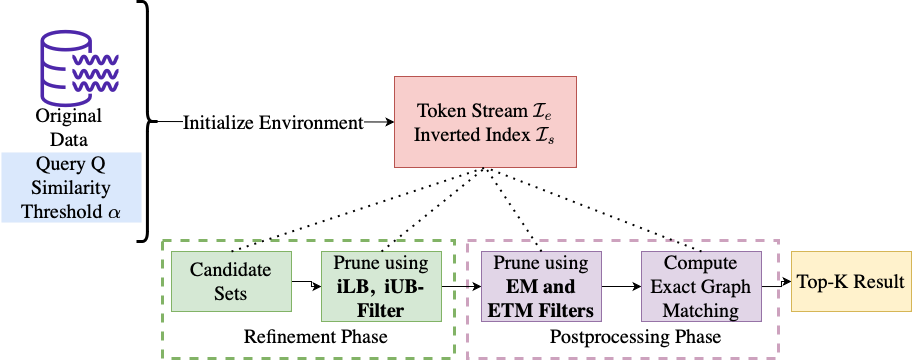
Our solution is a filter-verification algorithm, called Koios. In the refinement phase, Koios identifies candidate sets and aggressively prunes sets with no potential using cheap-to-apply filters. During post-processing, Koios takes pruning to the next level by only partially computing exact matches. Fig. 2 shows the basic framework of Koios.

Figure 2: Koios framework.

III Basic Filtering

We refer to the list of result sets partially ordered by semantic overlap descendingly as top-$k$ result and denote $\theta^{*}_{k}$ as the semantic overlap of the set with the $k$-th smallest semantic overlap in the top-$k$ result. Of course, the value of $\theta^{*}_{k}$ is not known until the top-$k$ result is computed. Assume an algorithm that iterates over sets in $\mathcal{L}$ and maintains a running top-$k$ list containing the best sets found so far: The running top-$k$ may contain any $k$-subset of $\mathcal{L}$ with non-zero semantic overlap. We denote the smallest semantic overlap of sets in the running top-$k$ list by $\theta_{k}$; by definition, $\theta_{k}\leq\theta^{*}_{k}$.

Based on Def. 1, any set $C\in\mathcal{L}$ that contains at least one element with similarity higher than $\alpha$ to some element of $Q$ has a non-zero semantic overlap and is a candidate set. Clearly, if $\mathcal{SO}(C)<\theta_{k}$, set $C$ can be pruned, as there exist at least $k$ sets with better $\mathcal{SO}$ scores. However, since computing $\mathcal{SO}(Q,C)$ is expensive (cubic in set cardinality), our goal during the refinement is to prune without computing the exact matching. To this end, we compute lower and upper bounds of the semantic overlap for candidate sets. The bounds help prune sets by comparing against the current $\theta_{k}$, hence, reducing the number of exact graph matching calculations.

UB-Filter: We define an upper bound for semantic overlap.

Lemma 2.

Given query set $Q$ and candidate set $C$, then $\mathcal{SO}(C)\leq|Q|\cdot\max_{q_{i}\in Q,c_{j}\in C}\{\mathrm{sim}(q_{i},c_{j})\}=UB(C)$.

Proof.

The weight of an edge, $(q_{i},c_{j})\in Q\times C$, in the semantic overlap bipartite graph of sets $Q$ and $C$ is bounded by the maximum similarity between any two elements of the sets. The size of any matching $M$ between $Q$ and $C$ is bound by $|M|\leq min(|Q|,|C|)\leq|Q|$. With Def. 1, $\mathcal{SO}(C)\leq UB(C)$. ∎

Since $UB(C)\leq\mathcal{SO}({\color[rgb]{0,0,0}C})$, any set $C$ that satisfies $UB(C)<\theta_{k}$ can be safely pruned with Lemma 2.

LB-Filter: Given a bipartite graph, the greedy matching algorithm at each iteration includes the edge with the highest weight between unmatched nodes until no edge with unmatched nodes can be found. The greedy algorithm for maximum matching has complexity $\mathcal{O}(n^{2}\cdot\log n)$, where $n$ is the cardinality of sets. As shown in Ex. 1, the greedy algorithm does not find the optimal solution. However, the score of the greedy matching has been shown to be at least half of the optimal score [18].

Lemma 3.

Let $Q$ and $C$ be two sets with semantic overlap $\mathcal{SO}(C)$. In the corresponding bipartite graph, let $LB(C)$ be the maximum of (a) the maximum edge weight, and (b) the greedy matching score. Then, $LB(C)\leq\mathcal{SO}(C)$.

Proof.

(a) We can always construct a one-to-one matching $M=\{(q_{i},c_{j})\}$ that consists of the edge $(q_{i},c_{j})$ with maximum weight. (b) Since the greedy matching of a bipartite graph is a lower bound of the optimal matching, $\mathcal{SO}(C)$ is lower-bounded by the greedy matching score. ∎

If we knew the value of $\theta^{*}_{k}$, we could do the maximum pruning during the refinement step. Initializing $\theta_{k}$ with a value close to $\theta_{k}^{*}$ will improve the prunig power of the UB-Filter. One way is to initialize the top-$k$ list by computing the $\mathcal{SO}$ of a sample of sets and picking the top-$k$ ones. In this case, the gained pruning power of the UB-Filter comes at the cost of graph matching calculations. To avoid this cost, we leverage a lower bound of $\theta_{k}$ for pruning.

Lemma 4.

Let $\mathcal{R}$ be the running top-$k$ list and $\theta_{lb}$ the smallest lower bound $LB(C)$ for $C\in\mathcal{R}$. Then, $\theta_{lb}\leq\theta^{*}_{k}$.

Proof.

By definition, $\theta_{lb}$ is the minimum $LB$ of sets in $\mathcal{R}$, and $\theta_{k}$ is the minimum exact $\mathcal{SO}$ of sets in $\mathcal{R}$. Since $LB(C)\leq\mathcal{SO}(C)$ for any set $C\in\mathcal{L}$, $\theta_{lb}=min_{C\in\mathcal{R}}\{LB(C)\}\leq min_{C\in\mathcal{R}}\{\mathcal{SO}(C)\}=\theta_{k}$ such that $\theta_{lb}\leq\theta_{k}\leq\theta^{*}_{k}$. ∎

With Lemma 4, we can safely prune a candidate set if $UB(C)<\theta_{lb}$.

IV Refinement: Candidate Selection

In the refinement phase, we use two index structures: the token stream $\mathcal{I}_{e}$ and the inverted index $\mathcal{I}_{s}$. Let $\mathbb{D}=\cup_{C_{j}\in\mathcal{L},c_{i}\in C_{j}}~{}c_{i}$, be the vocabulary of $\mathcal{L}$. The token stream $\mathcal{I}_{e}$ is a stream of all elements in $\mathbb{D}$ ordered in descending order by the maximum similarity to any query element $q_{i}\in Q$. The token stream $\mathcal{I}_{e}$ is a sequence of tuples $(q_{i},c_{j},\mathrm{sim}(q_{i},c_{j}))$, where $q_{i}\in Q$ and $c_{j}\in\mathbb{D}$. If $\mathrm{sim}(q_{i},c_{j})<\mathrm{sim}(q_{l},c_{m})$, tuple $(q_{i},c_{j},\mathrm{sim}(q_{i},c_{j}))$ will follow $(q_{l},c_{m},\mathrm{sim}(q_{l},c_{m}))$ in $\mathcal{I}_{e}$. The stream stops when there is no token $c_{j}\in\mathbb{D}$ left with $\mathrm{sim}(q_{i},c_{j})\geq\alpha,q_{i}\in Q$. The inverted index $\mathcal{I}_{s}$ maps $c_{j}\in\mathbb{D}$ to $\{C_{1},\ldots,C_{m}\}\subseteq\mathcal{L}$, such that $\forall~{}C_{i},1\leq i\leq m:c_{j}\in C_{i}$. Upon reading a tuple $(q_{i},c_{j},\mathrm{sim}(q_{i},c_{j}))$ from $\mathcal{I}_{e}$, the index $\mathcal{I}_{s}$ is probed to obtain all sets containing $c_{j}$. This creates a stream of sets in $\mathcal{L}$, in descending order of the maximum similarity set elements to some query element. Clearly, if a set appears in this stream it has a non-zero semantic overlap and is a candidate set. The first time we observe $C$ in this stream, $(q_{i},c_{j},\mathrm{sim}(q_{i},c_{j}))$ is in fact $\max\{\mathrm{sim}(q_{i},c_{j})\},c_{j}\in C,q_{i}\in Q$. Therefore, based on Lemma 2 and 3, we can initialize $UB(C)=min(|Q|,|C|)\cdot\mathrm{sim}(q_{i},c_{j})$ and $LB(C)=\mathrm{sim}(q_{i},c_{j})$. Koios uses the first $k$ sets obtained from $\mathcal{I}_{e}$ to initialize the running top-$k$ list and $\theta_{lb}$. As more sets are obtained, sets with lower $LB(C)$ may be found which results in updating the running top-$k$ list and $\theta_{lb}$.

Algorithm 1 presents the pseudo-code of the refinement phase of Koios. The power of the algorithm is in postponing exact match calculation to the post-processing phase, while pruning sets aggressively in this phase. In each iteration, Koios reads tuples from $\mathcal{I}_{e}$ and updates the bounds of candidate sets. Any set $C$ with $UB(C)<\theta_{lb}$ is safely pruned. A set $C$ with $LB(C)\leq\theta_{lb}\leq UB(C)$ is in limbo until more elements are read and more evidence about the bounds of the set is collected. The changes could be: $UB(C)$ decreases, $LB(C)$ increases, or $\theta_{lb}$ increases. The indexes $\mathcal{I}_{e}$ and $\mathcal{I}_{s}$ allow us to obtain candidate sets in the descending order of their initial upper- and lower-bounds. By processing candidate sets in this order, the search algorithm identifies promising sets early, can update the top-$k$ list, and improve $\theta_{lb}$ to achieve a high pruning ratio.

Due to Lemma 2, $UB(C)$ is tied to its largest element similarity to some query element. To order sets based on initial $UB$ and $LB$, we need to retrieve elements in the vocabulary $\mathbb{D}$ in descending order of their similarity to some query element. To avoid computing all pairwise similarities between vocabulary and query elements, for a given $\mathrm{sim}$, any index that enables efficient threshold-based similarity search is suitable. For example, when $\mathrm{sim}$ is the cosine similarity of word embeddings of tokens or the Jaccard of the token set of elements, the Faiss Index [19] or minhash LSH [20] can be plugged into the algorithm, respectively. This allows Koios to perform semantic overlap search independent of the choice of $\mathrm{sim}$. This sets Koios apart from existing fuzzy set similarity search techniques [13, 21, 22, 23], which rely on filters designed for specific similarity functions.

To retrieve candidate sets in the descending order of their upper-bounds, a naive solution is to extend the idea of the inverted index with a map that associates each query element to a list of all elements in the vocabulary. The elements in a list are ordered descendingly according to the similarity of an element to the query element. The size of this index grows linearly with the cardinality of $Q$. Now, let $r:Q\to\mathbb{A}$ be given by $r_{j}(q)=t^{j}$ for $j\in{1,\ldots,|\mathbb{D}|}$ that is to say that $r_{j}(q)$ returns the $j$-th most similar element of $\mathbb{D}$ to $q\in Q$. Note that the $j$-th most similar element to elements of $Q$ is not necessarily the one with $j$-th highest similarity to any element in $Q$, $\operatorname*{arg\,max}_{t^{j}}(\mathrm{sim}(t^{j},q_{i}),\forall i\in[Q])$. For example, $r_{i-1}(q)$ and $r_{i}(q)$ can both have higher similarities than $r_{1}(q^{\prime})$. The function $r$ can be realized by one shared index $\mathcal{I}$ over $\mathbb{D}$ and a priority queue $\mathcal{P}$ of size $|Q|$ that keeps track of the most similar elements to elements of $Q$. We refer to $\mathcal{I}$ and $\mathcal{P}$ as token stream $\mathcal{I}_{e}$.

Given an element $q$, the index $\mathcal{I}$ returns the next most similar unseen element of $\mathbb{D}$ to $q$. In the initial step, we probe $\mathcal{I}$ with all elements in $Q$ and add results to the priority queue. At this point, $\mathcal{P}$ contains $|Q|$ elements, each being the most similar element to a query element. The queue keeps track of the query element corresponding to each element in $\mathcal{P}$. The top of the queue always gives us the mapping of the query element to the unseen element with the highest similarity. The second most similar element to $Q$ is already buffered in $\mathcal{P}$. To maintain the queue size, when we pop the top element, we only require to probe $\mathcal{I}$ with the query element corresponding to the popped element because the most similar elements to the rest of the query elements still exist in $\mathcal{P}$. Note that when a non-zero $\alpha$ threshold is provided, we stop probing $\mathcal{I}$ when the first element with a similarity smaller than $\alpha$ is retrieved.

In addition, we build an inverted index that maps each element in $\mathbb{D}$ to the corresponding sets in $\mathcal{L}$. Since $\mathcal{I}_{e}$ returns elements in the descending order of similarity to $Q$, the new sets that are retrieved from $\mathcal{I}_{s}$ arrive at the descending order of UB-Filter.

Algorithm 1 Koios (Refinement)

1:$\mathcal{L}$: a repository, $\mathcal{I}_{e}$: token stream, $\mathcal{I}_{s}$: an inverted index on sets in $\mathcal{L}$, $Q$: a query set, $k$: search parameter, $\alpha$: token similarity threshold

2:$\mathcal{U}$: candidate sets

3:$\mathcal{U}\leftarrow\emptyset$, $\mathcal{P}\leftarrow\emptyset$ // candidate sets, pruned sets

4:$sim\leftarrow 1$ , $\mathcal{L}_{lb}\leftarrow\emptyset$ // initial similarity, top-$k$ LB list

5:while $sim\geq\alpha$ do

6:    $t,sim\leftarrow{\tt get\_next\_similar\_token(Q,\mathcal{I}_{e})}$

7:    if $sim\geq\mathcal{L}_{lb}.{\tt bottom}()$ then $Cs\leftarrow{\tt get\_sets(t,\mathcal{I}_{s})}$

8:        for $C\in Cs$ and $C\notin\mathcal{U}$ and $C\notin\mathcal{P}$ do $\mathcal{U}.{\tt add}$(C)             

9:    for $C\in\mathcal{U}$ do

10:        ${\tt UB}(C).{\tt update}(t,sim)$

11:        if ${\tt UB}(C)<\mathcal{L}_{lb}.{\tt bottom}()$ then

12:           $\mathcal{U}.{\tt remove}(C)$, $\mathcal{P}.{\tt add}(C)$         

13:        $LB(C).{\tt update}(t,~{}sim)$

14:        if $LB(C)>\mathcal{L}_{lb}.{\tt bottom}()$ then $\mathcal{L}_{lb}.{\tt update}(C)$             return $\mathcal{U}$

V Refinement: Advanced Filters

If a set obtained from the index is not pruned using the UB-Filter, it is added to the candidate collection. We introduce two advanced bounds, $iUB(C_{i})$ and $iLB(C_{i})$, and describe how we incrementally update these bounds. $iUB$ and $iLB$ are based on the partial bipartite greedy matching of sets. For an element in a candidate set, $\mathcal{I}_{e}$ may provide multiple matching elements (all edges in a bipartite graph). However, we only consider valid edges, i.e., those matching unmatched elements.

iLB: In $iLB$, we assume all edges that are not a part of a partial greedy matching have similarity zero.

Lemma 5.

Given candidate set $C$ and query $Q$, the sum of weights of any subset of edges in a bipartite greedy matching of $Q$ and $C$ is a lower-bound for $\mathcal{SO}(C)$.

Proof.

Let $G^{\prime}=(V,E^{\prime})$ be the bipartite graph of the greedy matching $M^{\prime}:Q\rightarrow C$ with score $s^{\prime}$. Suppose $M^{\prime\prime}:Q\rightarrow C$ is a matching with $G^{\prime\prime}=(V,E^{\prime\prime})$, where $E^{\prime\prime}\subseteq E^{\prime}$; let $s^{\prime\prime}$ be the score of $M^{\prime\prime}$. Because $E^{\prime\prime}\subseteq E^{\prime}$, we have $s^{\prime\prime}\leq s^{\prime}$. Based on Lemma 3, $s^{\prime}$ is a lower bound on $\mathcal{SO}(C)$, therefore, $s^{\prime\prime}\leq s^{\prime}\leq\mathcal{SO}(C)$. ∎

Suppose $iLB_{l}(C)$ is the current score of the partial greedy matching of $C$. Upon reading an unmatched element of $C$ with similarity $s_{l+1}$ to an unmatched query element, using Lemma 5, the lower-bound is updated to $iLB_{l+1}(C)=iLB_{l}(C)+s_{l+1}$. Since we obtain the edges of partial greedy matching from $\mathcal{I}_{s}$, we always consider the partial matching with the highest score, thus, computing the largest $iLB$. It is straightforward to verify if an $s_{l}$ must be included in the matching by keeping track of the set of elements that have been matched so far between $Q$ and each $C$. Updating the lower bound of a candidate set may result in updating the top-$k$ list and $\theta_{lb}$. Since $\theta_{lb}$ is always increasing (otherwise, we would not update), updating $\theta_{lb}$ results in pruning more sets based on their upper-bounds.

Since set $C$ may contain identical elements to query elements, i.e., $C\cap Q\neq\emptyset$ and the index returns elements in decreasing order, the lower-bound of $C$ is reduced to the number of its overlapping elements with the query, $|Q\cap C|$, plus the greedy matching score of the remaining elements of $Q$ and $C$. Because lower-bounds update $\theta_{lb}$, and a tighter $\theta_{lb}$ improves the pruning power of our technique, we choose to initialize the lower-bound of a set to its vanilla overlap (number of identical elements). To do so, the algorithm always includes a query element itself in the result of probing $\mathcal{I}_{e}$ for the first time. With this strategy, we deal with out-of-vocabulary elements. For example, if $\mathrm{sim}$ is the cosine similarity of the embedding vectors of tokens and some tokens are not covered in the embedding corpus, we still consider them in the semantic overlap calculation if the query contains the same tokens.

iUB-Filter: $iUB$ assumes the largest possible similarity for any edge that is not a part of a partial greedy matching, i.e., the smallest similarity seen so far from $\mathcal{I}_{e}$.

Lemma 6.

Given a partial greedy matching of cardinality $l$ of query $Q$ and set $C_{i}$ with score $S_{i}$. Upon obtaining $(q_{m},t,s)$ from $\mathcal{I}_{e}$, where $q_{m}\in Q$, element $t$ belongs to any set in $\mathcal{L}$, and $s$ is the next largest element pair similarity, we have the upper bound $iUB(C_{i})=S_{i}+min(|Q|-l,|C_{i}|-l)\cdot s\geq\mathcal{SO}(C_{i})$.

Proof.

Since $l$ elements of $C_{i}$ have already been matched to elements of $Q$, set $C_{i}$ has maximum $m_{i}=min(|Q|-l,|C_{i}|-l)$ remaining elements to be matched. Upon reading an element $t$, with the next largest similarity, namely $s$, regardless of which set $t$ belongs to, by definition, any unseen element of $C_{i}$ has similarity smaller than or equal to $s$. There are two scenarios: either element $t\in C_{i}$ or $t\notin C_{i}$. If $t\in C_{i}$ is already matched with some element in the query, we discard the element and know that any unmatched element has a similarity no larger than $s$ to a query element. Otherwise, the upper-bound of any unmatched element in $C_{i}$ after observing element $t$ can be tightened to $s$ and we have $iUB(C_{i})=S_{i}+m_{i}\cdot s$. ∎

Updating $iUB(C_{i})$ can result in pruning the set if $S_{i}+m_{i}~{}.~{}s\leq\theta_{lb}$. A naive way is to update the upper-bound of all sets, whenever a new element is retrieved from $\mathcal{I}_{e}$. However, this results in an excessive number of small updates many of which will not sufficiently decrease the upper-bound to prune the updated set. To solve this issue, we propose a technique that groups sets into buckets by their number of unseen elements ($m$). Only sets that contain a newly retrieved element require an update and are moved to bucket $m-1$. All other sets need not be updated, but still are pruned as soon as their upper-bound falls below $\theta_{lb}$.

Koios bucketizes sets into $m$ buckets $B_{m}=\{(C_{i},S_{i})|m_{i}=m\}$. Upon the arrival of a new element with similarity $s$, any set $C_{i}$ in $B_{m}$ and a sum of matched elements $S_{i}$ should be pruned if its updated upper-bound is smaller than $\theta_{lb}$, i.e. $S_{i}+m\cdot s\leq\theta_{lb}$. We conclude that if $S_{i}\leq\theta_{lb}-(m\cdot s)$, we can safely prune $C_{i}$. Since all sets in a bucket have the same number of remaining elements and $s$ is fixed for all sets, the right-hand side of this pruning inequality is the same for all sets in a bucket.

We maintain the pairs $(C_{i},S_{i})$ in a bucket ordered by ascending $S_{i}$ values. Upon the arrival of an element with similarity $s$, we scan the ordered list of sets in each bucket. If a pair satisfies the condition $S_{i}\leq\theta_{lb}-(m\cdot s)$, we prune the set. As soon as we find a set $S^{\prime}$ that does not satisfy the condition, we can conclude that the remaining sets do not satisfy the condition and cannot be pruned, because the remaining sets must have $S_{i}$ values larger than $S^{\prime}$. Now, suppose a set $C_{i}$ in bucket $B_{m}$ contains the newly arrived element: We first remove the pair $(C_{i},S_{i})$ from its bucket, update $S_{i}$, and insert the pair into $B_{m-1}$. Restricting updates to the sets that contain an element and using the element similarity to prune some sets saves us many updates at each iteration. Our experiments confirm that maintaining buckets does not incur a large overhead.

Since the similarity of identical elements is one even for identical out-of-vocabulary elements, like $iLB$, Koios initializes the upper-bound of a newly obtained set $C_{i}$ and its $S_{i}$ to its vanilla overlap.

Figure 3: Pruning sets with upper and lower bounds for $k=2$. Each set is represented with its LB and UB. The red circles indicate the pruned sets and the green lines indicate the recent updates to LB and UB.

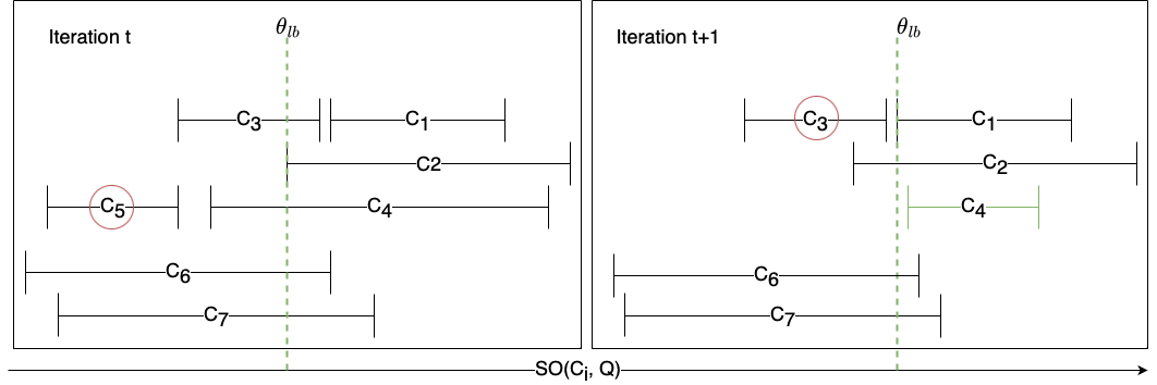
Example 3: Consider sets $C_{1},\ldots,C_{7}$ in Fig. 3. Suppose we are searching for the top-$2$ sets with the highest semantic overlap with a query. Each set is represented with an interval of its lower-bound and upper-bound with respect to the query. The value of $\theta_{lb}$ is initially calculated based on the lower-bounds of $C_{1}$ and $C_{2}$, since they have the top-$2$ lower bounds among all sets. This means at the beginning of iteration $t$, set $C_{5}$ is pruned because $UB(C_{5})<\theta_{lb}$. The remaining sets stay in the candidate collection because they all have lower-bounds smaller than $\theta_{lb}$ and upper-bounds that are greater than $\theta_{lb}$. Suppose, at iteration $t+1$, by reading an element of $C_{4}$ from the token stream, $LB(C_{4})$ and $UB(C_{4})$ are updated (the right side of Fig. 3). Now, $C_{4}$ is the set with the highest lower bound and as a result, the value of $\theta_{lb}$ is updated to $LB(C_{1})$. This allows us to safely prune $C_{3}$ because $UB(C_{3})<\theta_{lb}$. At the end of the refinement phase, the algorithm passes remaining sets ($C_{1}$, $C_{2}$, $C_{4}$, $C_{6}$, and $C_{7}$) to the post-processing phase. $\Box$

VI Post–Processing Phase

All candidate sets that have not been pruned during the refinement need to be verified. Some sets may end up in this phase due to their large cardinality even though the similarity of their elements is relatively low. Koios applies filters during post-processing to minimize the number of exact match calculations as well as the time to complete the calculation.

No-EM: Let $\mathcal{U}$ be the candidate sets that have not been pruned, and $\theta_{ub}$ be the $k$-th largest $UB(C)$ for $C\in\mathcal{U}$.

Lemma 7.

A set $C\in\mathcal{U}$ with $\theta_{ub}\leq LB(C)$ is guaranteed to be in a top-$k$ result $\omega$.

Proof.

Computing the maximum graph matching for a $C\in\mathcal{U}$ never increases $\theta_{ub}$, because $\mathcal{SO}(C)\leq UB(C)$. If a set $C\in\mathcal{U}$ satisfies $\theta_{ub}\leq LB(C)$, by $LB(C)\leq UB(C)$ and $\theta^{*}_{k}\leq\theta_{ub}$, it is guaranteed that $\theta^{*}_{k}\leq\mathcal{SO}(C)$ and $C$ is in the top-$k$ result. ∎

This Lemma allows us to skip the exact semantic overlap calculation of some sets. Due to ties at distance $\theta_{k}^{*}$ from the query there can be multiple solutions for the top-$k$ search problem. All solutions share the same value for $\theta_{k}^{*}$.

Algorithm 2 Koios (PostProcessing)

1:$Q$: a query set, $k$: search parameter, $\mathcal{U}$: unpruned sets, $k$: search parameter, $\mathcal{L}_{lb}$: top-$k$ LB list

2:$\mathcal{L}_{ub}$: top-$k$ results

3:$\mathcal{Q}_{ub}\leftarrow{\tt init\_pq\_UB(\mathcal{U})}$ // priority queue on unpruned sets

4:$\mathcal{L}_{ub}\leftarrow{\tt init\_topk\_UB(\mathcal{U})}$ // top-$k$ UB list on unpruned sets

5:while $\neg\mathcal{L}_{ub}.{\tt all\_checked()}$ do

6:    $C\leftarrow\mathcal{L}_{ub}.{\tt select\_next\_unchecked}()$

7:    if $LB(C)\geq UB(\mathcal{L}_{ub}.{\tt top}())$ then

8:        C.${\tt checked}\leftarrow$True

9:        continue     

10:    SO(C)$\leftarrow$compute_SO_early_termination(C,Q)

11:    LB(C),UB(C)$\leftarrow$SO(C), C.${\tt checked}\leftarrow$True

12:    if $SO(C)<\mathcal{L}_{ub}.{\tt bottom}()$ then $\mathcal{L}_{ub}.{\tt remove}(C)$

13:        if $SO(C)\geq\mathcal{L}_{lb}.{\tt bottom}()$ then $\mathcal{Q}_{ub}.{\tt add}(C)$             

14:    if $SO(C)\geq\mathcal{L}_{lb}.{\tt bottom}()$ then $\mathcal{L}_{lb}.{\tt update}(C)$     

15:    while $\mathcal{L}_{ub}.{\tt len}()<k$ and $\neg\mathcal{Q}_{ub}.{\tt empty()}$ do

16:        $C\leftarrow\mathcal{Q}_{ub}.{\tt pop}()$

17:        if $\mathcal{L}_{lb}.{\tt bottom}()<UB(C)$ then $\mathcal{L}_{ub}.{\tt add}(C)$             return $\mathcal{L}_{ub}$

In this phase, Koios maintains three data structures: 1) an ordered list of sets with top-$k$ lower-bounds ($\mathcal{L}_{lb}$), 2) an ordered list of sets with top-$k$ upper-bounds ($\mathcal{L}_{ub}$), and 3) a priority queue of sets ordered by upper-bounds ($\mathcal{Q}_{ub}$). Maintaining $\mathcal{L}_{lb}$ and $\mathcal{L}_{ub}$ allows us to have fast access to $\theta_{lb}$ and $\theta_{ub}$, respectively. Based on Lemma 7, the algorithm should only compute the bipartite matching of sets with $UB(C)\geq\theta_{ub}$. As such, Koios prioritizes the exact graph-matching calculation of sets with high upper-bounds. Intuitively, sets with high upper-bounds have the potential for high semantic overlaps. To speed up, all sets in $\mathcal{L}_{ub}$ are queued and evaluated in parallel in the background. Upon the completion of the exact match of a set $C$, we update $LB(C)=UB(C)=\mathcal{SO}(C)$. This has two effects. First, the update of $UB(C)=\mathcal{SO}(C)$ may cause the $\theta_{ub}$ to be decreased. As a result, if $\mathcal{SO}(C)\geq\theta_{ub}$, the set remains in $\mathcal{L}_{ub}$. If $\mathcal{SO}(C)<\theta_{ub}$, we add the set to $\mathcal{Q}_{ub}$, because the algorithm may realize later that $\mathcal{SO}(C)$ was higher than the sets that are currently in $\mathcal{L}_{ub}$, whose semantic overlaps are not calculated yet. Inserting a set into $\mathcal{Q}_{ub}$ results in $\mathcal{L}_{ub}$ having $k-1$ sets. Probing $\mathcal{Q}_{ub}$ provides the next set with the $k$-th largest upper-bound to be added to $\mathcal{L}_{ub}$.

Second, the update of $LB(C)$ may cause the $\theta_{lb}$ to increase and potentially prune some sets. The algorithm takes a lazy approach and considers the sets in $\mathcal{L}_{ub}$ for such pruning until a set $C$ with $UB(C)\leq\theta_{lb}$ is obtained. The post-processing phase terminates when all sets in the $\mathcal{L}_{ub}$ satisfy the condition $\theta_{ub}\leq LB(C)$ and the list is returned as the final search result.

EM-Early-Terminated-Filter: Despite pruning sets extensively, the exact matching calculation remains expensive. Consider bipartite graph $G(V,E)$ built on $C$ and $Q$, where $V={Q}\uplus{C}$ and the weight of an edge between elements $q_{i}\in Q$ and $c_{j}\in C$ is $w(q_{i},c_{j})=\mathrm{sim}(q_{i},c_{j})$. The weight of an optional one-to-one matching $M\subseteq E$ is $w(M)=\sum_{(q_{i},c_{j})\in M}w(q_{i},c_{j})$. A matching $M$ is called perfect if for every $v\in V$, there is some $e\in M$ which is incident on $v$. The Hungarian algorithm [24] considers a node labeling to be a function $l:V\rightarrow\mathbb{R}$. A feasible labeling satisfies $l(q_{i})+l(c_{j})\geq w(q_{i},c_{j}),\forall q_{i}\in Q,c_{j}\in C$. An equality subgraph is a subgraph $G_{l}=(V,E_{l})\subset G=(V,E)$, fixed on a labeling $l$, such that $E_{l}=\{(q_{i},c_{j})\in E:l(q_{i})+l(c_{j})=w(q_{i},c_{j})\}$. The Hungarian algorithm considers a valid labeling function $l$ and maintains a matching $M$ and a graph $G_{l}$. It starts with $M=\emptyset$. At each iteration, the algorithm either augments $M$ or improves the labeling $l\rightarrow l^{\prime}$ until $M$ becomes a perfect matching on $G_{l}$. Let $M^{\prime}$ be a perfect matching in $G$ (not necessarily in $G_{l}$). It is a well-known result that if $l$ is feasible and $M$ is a perfect matching in $G_{l}$, then $M$ is a maximum weight matching [24]. From the proof of the Kuhn-Munkres theorem, we have that $w(M^{\prime})\leq w(M)$. This theorem also shows that for any feasible labeling $l$ and any matching $M$ we have $w(M)\leq\sum_{v\in V}l(v)$ [24].

Lemma 8.

A set $C$ can be safely pruned during bipartite graph matching with $Q$ if the sum of labels assigned by the Hungarian algorithm [24] is smaller than $\theta_{lb}$.

Proof.

Suppose a valid node labeling function $l$ and an equality subgraph $G_{l}$. The perfect matching $M$ on $G_{l}$ created by the Hungarian algorithm is indeed the maximum matching and its weight $w(M)$ is the semantic overlap of $Q$ and $C$. Now, let $M^{\prime}$ be some perfect matching in $G$. Since from the Kuhn-Munkres theorem we know that $w(M^{\prime})\leq w(M)$ and for the labeling $l$ and matching $M$, $w(M)\leq\sum_{v\in V}l(v)$, we have $w(M^{\prime})\leq\sum_{v\in V}l(v)$. Therefore, the sum of node labels is an upper bound for $\mathcal{SO}(Q,C)\leq\sum_{v\in V}l(v)$. This upper bound can be computed on the fly during graph matching. A set $C$ can be pruned as soon as $\sum_{v\in V}l(v)$ exceeds $\theta_{lb}$. ∎

By computing this upper-bound during the process of graph matching for a set $C$, as soon as $UB(C)<\theta_{lb}$, the process can be terminated and $C$ can be safely removed. The early termination is particularly important for large sets when the matching of a large set is executed in parallel and a global $\theta_{lb}$ is updated as the processing of other sets is completed.

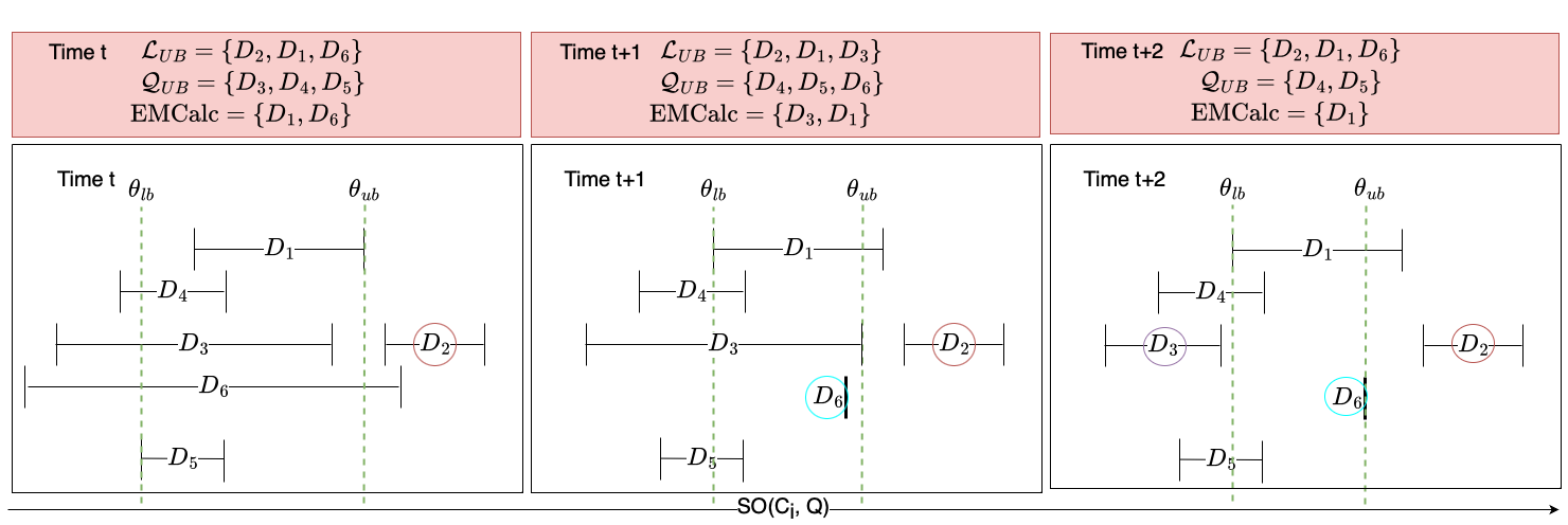
Example 4: Suppose sets $D_{1}$, $\ldots$, $D_{6}$ of Fig. 4 are in the post-processing phase. Suppose we are searching for the top-$3$ sets. Each set is represented with an interval of its lower-bound and upper-bound with respect to the query. The post-processing starts by $\mathcal{L}_{ub}=[D_{2},D_{1},D_{6}]$. From $LB(D_{2})>\theta_{ub}$, we know we do not need to compute the exact match of $D_{2}$, because we know the true value of $\theta_{k}$ ($\theta^{*}_{k}$) is never greater than $\theta_{ub}$. Thus, any set with semantic overlap higher than $\theta^{*}_{k}$ must be in the final result. The exact matching of $D_{1}$ and $D_{6}$ are calculated in parallel. Suppose $D_{6}$ finishes and its bounds are updated. This results in increasing $\theta_{lb}$ and decreasing $\theta_{ub}$. Thus, $D_{6}$ is removed from $\mathcal{L}_{ub}$ and added to $\mathcal{Q}_{ub}$. After probing $\mathcal{Q}_{ub}$ considering $\theta_{lb}$, $D_{3}$ is added to $\mathcal{L}_{ub}$. Suppose using the early termination rule, $UB(D_{3})$ is updated to a value lower than $\theta_{lb}$. The algorithm immediately stops the matching of $D_{3}$, and eliminates it from $\mathcal{L}_{ub}$. At this point, $D_{6}$ is added back to $\mathcal{L}_{ub}$ and $\theta_{ub}=SO(D_{6})$. The algorithm continues to compute the next set in $\mathcal{L}_{ub}$ ($D_{1}$). $\Box$

Figure 4: Post-processing: pruning sets with upper and lower-bounds and exact semantic overlap, for $k=3$. Each set is represented with its LB and UB. Here the red circle indicates NoEM Filter, the blue circle indicates EM, and the purple circle indicates the EM-ETM Filter.

To scale out search, we randomly partition the repository and run Koios on partitions in parallel. To improve the pruning power, all partitions share a global $\theta_{lb}$ that is the maximum of the $\theta_{lb}$.

VII Analysis of Koios

VII-A Correctness

Based on Def. 1, a set $C$ with at least one element with similarity greater than $\alpha$ has a non-zero semantic overlap with $Q$. The token stream retrieves all set elements with similarity greater than $\alpha$, and for each element, the inverted index returns all sets containing that element. As a result, all sets with non-zero semantic overlap are considered. Koios can prune a set $C$ under three circumstances: (1) When $C$ appears for the first time due to the similarity $s$ of one of its elements $c_{j}\in C$ to some query element $q_{i}\in Q$. Because of the non-increasing similarity order in $\mathcal{I}_{e}$, $s=\max\{\mathrm{sim}(q_{i},c_{j})\},c_{j}\in C,q_{i}\in Q$. Therefore, based on Lemma 2 , the upper bound $UB(C)$ can be computed, and $C$ is pruned if $UB(C)\leq\theta_{lb}$. Note that considering $\theta_{lb}$ for pruning does not create false negatives because, as shown in Lemma 4, $\theta_{lb}\leq\theta_{k}\leq\theta^{*}_{k}$. (2) During refinement by iUB filter: Lemma 6 proves an upper bound based on the similarity of elements of arbitrary sets, thus any set pruned by $\theta_{lb}$ cannot be a false negative. (3) During post-processing: Lemma 8 proves that whenever the sum of node labels of the Hungarian algorithm becomes smaller than $\theta_{lb}$, the set can be safely pruned. The algorithm continues to prune based on the UB-Filter in this phase as $\theta_{lb}$ is being improved by the exact match calculation. If a set is not pruned under the above conditions until the algorithm terminates, it remains in $\mathcal{L}_{ub}$ and is in fact in the top-$k$ result.

VII-B Time and Space Complexity

The exact bipartite graph matching can be computed in $\mathcal{O}(n^{3})$ time [25, 26]. Although the worst-case time complexity of Koios is $\mathcal{O}(m\cdot n^{3})$, where $n$ is the maximum set cardinality and $m$ is the number of sets in $\mathcal{L}$, thanks to our filters we require far fewer than $m$ comparisons, thereby reducing the overall runtime by orders of magnitude in practice. Moreover, the EM-early-terminated filter can reduce the number of iterations of the Hungarian algorithm.

Recall that $\mathbb{D}$ is the vocabulary of all distinct tokens in $\mathcal{L}$. Each token in $Q$ can have a similarity greater than $\alpha$ with at most $\lvert\mathbb{D}\rvert$ tokens, thus the space complexity for the token stream $\mathcal{I}_{e}$ is $\mathcal{O}\left(\lvert\mathbb{D}\rvert\cdot\lvert Q\rvert\right)$. The inverted index $\mathcal{I}_{s}$ is linear in the input size: it stores $\lvert\mathbb{D}\rvert$ keys and the aggregate size of all lists is at most $D^{+}=\sum_{C\in\mathcal{L}}\lvert C\rvert$. With $\lvert\mathbb{D}\rvert\leq D^{+}$ and an average set size of $\bar{C}$, the space complexity of $\mathcal{I}_{s}$ is $\mathcal{O}\left(\mathcal{L}\cdot\bar{C}\right)$. Both the top-$k$ lists, $\mathcal{L}_{lb}$ and $\mathcal{L}_{ub}$, store at most $k$ sets at any given time during the iteration and have a space complexity of $\mathcal{O}\left(k\right)$. The size of the priority queue $\mathcal{Q}_{ub}$ is $\mathcal{O}\left(\mathcal{L}\right)$. This gives us the overall space complexity of $\mathcal{O}\left(\lvert\mathbb{D}\rvert\cdot\lvert Q\rvert+\mathcal{L}\cdot\bar{C}\right)$.

TABLE I: Characteristics of datasets.

	#Sets	MaxSize	AvgSize	#UniqElems
DBLP	4,246	514	178.7	25,159
OpenData	15,636	31,901	86.4	179,830
Twitter	27,204	151	22.6	72,910
WDC	1,014,369	10,240	30.6	328,357

VIII Experiments

We evaluate the response time, memory footprint, and pruning power of filters of Koios on four real-world datasets and test various parameter settings and query cardinalities. We compare Koios with a baseline and a state-of-the-art fuzzy set similarity search technique. The usefulness of semantic overlap measure for search is evaluated by comparing to the results of vanilla set overlap search. In our experiments, we use the cosine similarity of the embedding vectors of tokens using pre-trained vectors of FastText [28] as the function $\mathrm{sim}$.

VIII-A Experimental Setup

VIII-A1 Datasets

We use four datasets: DBLP [29], OpenData [30], Twitter [31], and the public corpus of WebTables (WDC) [32]. For DBLP, we consider papers from 2018 and 2019, and for each publication, we generate a set of white-spaced words from the paper title and abstract. For each English tweet in the Twitter dataset, we generate a set consisting of the distinct words in the tweet except the emojis and URLs. The sets for OpenData and WDC are formed by the distinct values in every column of every table. For all datasets, we remove numerical values to avoid casual matches. We further filter OpenData and WDC by discarding all sets that have less than 70% coverage of pre-trained vectors. The characteristics of the extracted sets are shown in Table I. The majority of sets in WDC and Twitter are small but they contain more sets compared to OpenData and DBLP. Unlike in OpenData, there are some very frequent elements in WDC, which results in excessively large posting lists in the inverted index. As a result, the number of candidate sets in WDC during the refinement is large, and updating the bounds of the sets is often more expensive in WDC than OpenData.

VIII-A2 Benchmarks

We generated one query benchmark, i.e., a collection of query sets, from each data set. The set cardinalities in WDC and OpenData are highly skewed [8]. In order to evaluate the performance depending on the query cardinality, the benchmarks of WDC and OpenData are collections of query sets selected from different cardinality ranges. The ranges for OpenData are: 10 to 750, 750 to 1000, 1000 to 1500, 1500 to 2500, 2500 to 5k, and 5k to 32k; the intervals for WDC are: 10 to 250, 250 to 500, 500 to 750, 750 to 1k, and 1k to 11k. For each interval, we sample $50$ and $100$ sets using uniform random sampling for OpenData and WDC respectively. Sampling by interval prevents the benchmarks from being biased towards small sets. Large intervals are used for high cardinality sets due to the power-law distribution of the set cardinalities [7]. Since DBLP and Twitter contain fewer skewed sets, we do not create intervals and draw 100 random sets using uniform sampling. We report the average of results over the queries for each benchmark and interval.

VIII-A3 Implementation

The inverted index ($\mathcal{I}_{s}$) is computed on the fly and stored in an in-memory hash map. To generate the token stream we use the GPU implementation of the top-$k$ Faiss index [19] over high-dimensional vectors. We query the Faiss index in batches of 100 elements. The construction time of the inverted index is $1.5$, $3.0$, $1.3$, and $80$ seconds, and the construction time of Faiss index is $3.6$, $9.5$, $3.8$, $12.5$ seconds for DBLP, OpenData, Twitter, and WDC respectively. We cache the similarity of returned vectors during the refinement phase for reuse during the initialization of the similarity matrix used in graph matching. For graph matching, we use an implementation of the Hungarian algorithm [33]. To compute the graph matching of sets in parallel during the post-processing phase, we use a C++17-compatible thread pool implementation [34]. Unless otherwise specified, the following parameters are used in all experiments: similarity threshold $\alpha=0.8$, k = $10$, and partitions = $10$.

VIII-A4 Baselines

The baseline approach for top-$k$ semantic overlap search iterates over all candidate sets and computes their bipartite graph matchings. Candidate sets are those that have at least one element with similarity to any query elements greater than the threshold $\alpha$. We use the token stream to get a list of candidate sets (baseline’s refinement phase) and use a thread pool [34] to parallelize the computation of the graph matching of all candidate sets (baseline’s post-processing). Given the sheer number of sets and high frequency of elements in WDC, computing exact graph matchings for all candidate sets is infeasible. For example, we have $190,679$ candidate sets for a query set with cardinality $53$. To reduce the number of candidate sets, we activate the iUB-Filter to assist with set pruning. This is referred to as Baseline+.

VIII-A5 System Specifications

All experiments are conducted on a machine with 2 Intel^® Xeon Gold 5218 @ 2.30GHz (64 cores), 512 GB DDR4 memory, a Samsung^® SSD 983 DCT M.2 (2 TB), 4 GPUs - TU102 (GeForce RTX 2080 Ti).

(a)

(b)

(c)

(d)

Figure 5: OpenData results: (a) response time, (b), (c) phase breakdown, (d) memory footprint.

(a)

(b)

(c)

(d)

Figure 6: WDC results: (a) response time, (b), (c) phase breakdown, (d) memory footprint.

TABLE II: Average percentage of sets pruned using filters.

Datasets	Refinement	Postprocessing
	iUB-Filter	EM-Early-Terminated	No-EM
DBLP	$91\%$	$5\%$	$9.2\%$
OpenData	$85.5\%$	$2.1\%$	$54.8\%$
Twitter	$53.5\%$	$0\%$	$1.4\%$
WDC	$89.2\%$	$0.9\%$	$9.8\%$

TABLE III: Average response time and memory footprint.

	Koios				Baseline
Datasets	Refinement	Postproc	Response	Mem	Response	Mem
	(sec)	(sec)	(sec)	(MB)	(sec)	(MB)
DBLP	$0.3$	$0.44$	$0.83$	$16$	$211$	$11$
OpenData	$7.19$	$6.9$	$18.6$	$69.6$	$101$	$102.5$
Twitter	$0.2$	$0.45$	$0.7$	$10$	$518$	$10$
WDC	$109$	$34.3$	$147$	$1,775$	$1,062$	$885$

VIII-B Response Time

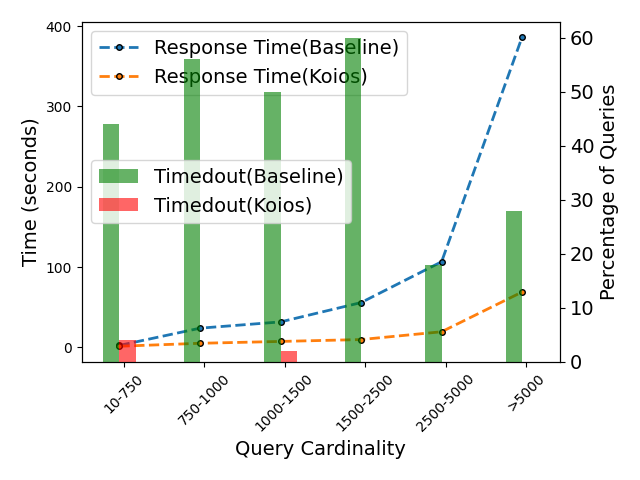
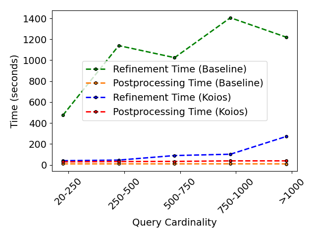
We report the average response time, in seconds, across benchmarks for all datasets in Table III (inverted index and token index construction time are excluded from § VIII-A3). We do not report the time for the timed-out queries ($2500$ seconds), therefore, we do not have enough data for some intervals of WDC and OpenData. According to Table III, Koios achieves at least 5x speedup over the baseline across all datasets and at least 200x for DBLP and Twitter. We present additional analyses of WDC and OpenData based on query cardinality, since these datasets demonstrate a large set cardinality skew.

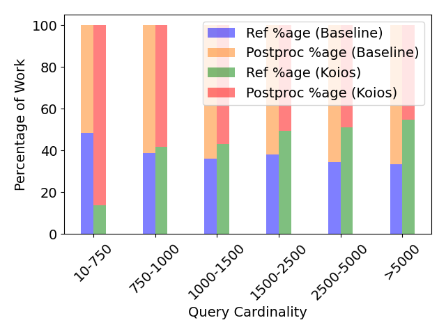
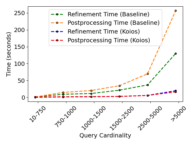
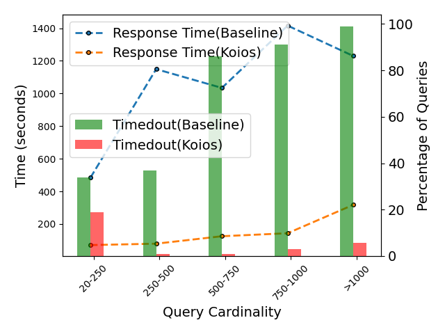
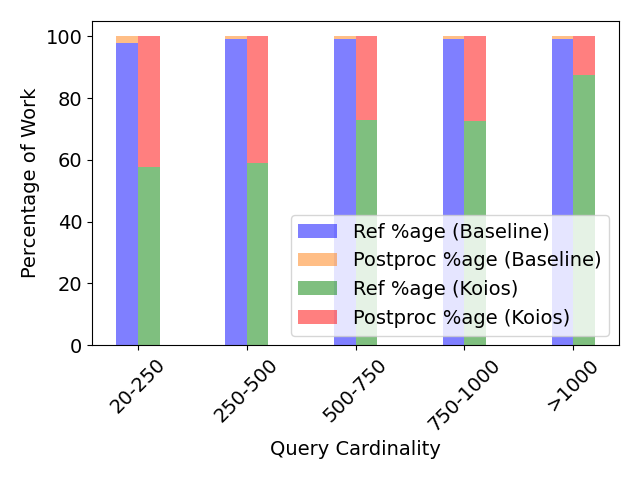
Effect of Query Cardinality: Fig. 5(a), 5(b), 6(a), and 6(b) show the response time and the relative time spent in each phase for OpenData and WDC, respectively. The time reported is averaged over all queries in each interval. Because Koios processes all partitions in parallel, we report the average ratio of time spent by a partition over all queries in an interval. We observe that the response time increases with query cardinality, which entails a larger number of similar elements and candidate sets returned by $\mathcal{I}_{s}$. The share of work of WDC in the refinement is higher than OpenData, because of its sheer number of sets and the high frequency of elements.

Comparing to Baseline: Fig. 5(a) and 6(a) show that Koios particularly outperforms the baseline for medium to large queries in OpenData and WDC. This emphasizes the pruning power of the filters. Fig. 5(a) and 6(a) also report the number of timed-out queries which are much higher for the baseline than for Koios, since the baseline does not prune the large low potential sets in the refinement phase. Koios times out for only approximately $5\%$ of OpenData queries and approximately $20\%$ of WDC queries for small queries. This is due to the large posting lists, which result in a significant number of sets during post-processing as visible from Tables IV and V. We also note that Koios times out for certain medium-large queries, which is due to expensive graph matching. In summary, the filter overhead of Koios during refinement clearly pays off and significantly improves the runtime over the baseline. We remark that Koios finds $k\times\left(\text{number of partitions}\right)$ sets significantly faster than the time-out limit, whereas the majority of large queries for WDC time out for the baseline. Although the difference in response time of Koios and baseline is not prominent for smaller queries of OpenData, Koios discovers $k\times\left(\text{number of partitions}\right)$ sets as opposed to the baseline.

Comparing to Fuzzy Search: Fuzzy search techniques including Fast-Join[11, 12] and SILKMOTH [13] cannot solve the top-$k$ overlap similarity search problem that we solve in this paper: (1) Only specific character-level similarities (Jaccard on white-space separated tokens of an element and edit distance) between set elements are supported; semantic similarity like cosine on word embeddings (as we use in our experiments) cannot be applied. (2) Existing fuzzy search algorithms are threshold-based: In order to retrieve the top-$k$ most similar sets to a given query, the threshold $\theta^{*}_{k}$ is required, but this threshold is not known upfront; in fact, it is one of the challenges of top-$k$ search and part of our solution to converge to this threshold quickly.

While fuzzy search algorithms do not support semantic element similarity, our KOIOS algorithm does support all syntactic element similarity functions. We extend the threshold-based fuzzy search to support top-$k$ search as follows: (1) Pick the threshold $\theta$ as the minimum $\theta^{*}_{k}$ amongst all the queries. Note this gives SILKMOTH an advantage as we pass the true value of $\theta^{*}_{k}$ (2) Compute the fuzzy search with threshold $\theta$ and select the top-$k$ most similar sets from the query result (by maintaining a top-$k$ priority queue).

We focus our study on SILKMOTH, which was shown to widely outperform Fast-Join [13] and consider OpenData and WDC datasets. Since sets in these datasets are extracted from tables, the majority of elements consist of very few words, which results in a zero edge weight for non-identical elements in SILKMOTH. Therefore, in our experiments, we consider Jaccard on $3$-grams representation of each element as an element similarity for both Koios and SILKMOTH. To generate the token stream, we precompute elements in the vocabulary that are similar to each query element with the Jaccard similarity threshold of $\alpha=0.8$, using the set similarity join techniques [9]. It takes $8$ seconds to compute the token stream for the benchmark.

We compare two versions of SILKMOTH: The first version, SILKMOTH-semantic, adapts the SILKMOTH algorithm to cover most of the functionality of Koios ; this adaption was suggested by the original authors as a generic search framework and excludes similarity function specific filters [13]. The second version, SILKMOTH-syntactic, uses all indexes and filters, including those that are applicable only to particular similarity functions. We run the algorithms on 54 queries randomly sampled from the benchmark queries of OpenData to make sure we evaluate on small, medium, and large sets and measure response time. The average response time of Koios, SILKMOTH-syntactic, and SILKMOTH-semantic are $72$, $141$, and $400$ seconds, respectively. Koios outperforms both SILKMOTH-semantic, and SILKMOTH-syntactic by an order of magnitude $6$x(timed-out), and $2$x respectively on all query size ranges. SILKMOTH produces signatures from the set elements and utilizes them to help decrease the candidate space. The number of signatures increases when the number of set elements increases (here by splitting into $q$-grams) and SILKMOTH-syntactic times out due to the sheer number of viable candidates. Koios outperforms SILKMOTH-syntactic because it operates on an ordered stream of set element pairings based on similarity and is thus unaffected by the number of elements. Koios outperforms SILKMOTH-semantic because the pruning power of SILKMOTH is highly dependent on filters that are specialized for certain similarity functions.

VIII-C Pruning Power of Filters

Table II reports the mean pruning power of different filters used in both phases for all datasets and Tables IV and V zooms into the pruning power for OpenData and WDC across query cardinality intervals.

Refinement Phase: In OpenData and WDC, the number of candidate sets increases with query cardinality because more posting lists from $\mathcal{I}_{s}$ must be read. The pruning power of the iUB-filter increases with the increase of query cardinality. This is because of two reasons, first, there are a significant amount of small cardinality sets in OpenData and WDC (Table I), that are returned by the posting lists. Second, the iUB of each set is calculated based on the number of remaining elements, thus candidate sets with smaller cardinality relative to the query set have a much smaller iUB as compared to the $\theta_{lb}$ and are hence pruned. As shown in the Tables IV and V, although the number of candidate sets increases with query cardinality, the fraction that requires post-processing by Koios decreases with query cardinality. For example, Koios requires the post-processing of less than 5% of candidate sets for large queries for WDC.

(a)

(b)

(c)

(d)

Figure 7: Parameter analysis of Koios on OpenData: Time vs. (a) number of partitions, (b) element similarity ($\alpha$), and (c) result size, (d) memory footprint vs. alpha.

Post-processing Phase: Table II shows that the No-EM filter demonstrates a higher pruning power than EM-Early-Terminated, e.g., pruning more than half of sets for OpenData. Note that the reported percentages refer to the sets that are not filtered in the refinement phase. From Tables IV and V we observe that the combination of No-EM and EM-Early-Terminated have the highest pruning power for large queries. For OpenData, the combination of these two filters prunes more sets than in WDC. This is because an exact calculation of semantic overlap during the post-processing increases $\theta_{k}$ and results in pruning many sets.

TABLE IV: OpenData: #sets pruned by filters.

	Refinement Phase		Postprocessing Phase
Query Card.	Candidate	iUB-Filtered	No-EM	EM-Early	EM
	Sets			Terminated
$10-750$	$1132$	$345$	$88$	$0$	$699$
$750-1000$	$2557$	$2422$	$85$	$2$	$48$
$1000-1500$	$2699$	$2571$	$83$	$4$	$41$
$1500-2500$	$3440$	$3328$	$84$	$2$	$26$
$2500-5000$	$3560$	$3451$	$82$	$4$	$23$
$>5000$	$5706$	$5502$	$79$	$5$	$120$

TABLE V: WDC: #sets pruned by filters.

	Refinement Phase		Postprocessing Phase
Query Card.	Candidate	iUB-Filtered	No-EM	EM-Early	EM
	Sets			Terminated
$20-250$	$124,217$	$60,196$	$74$	$80$	$63,867$
$250-500$	$189,665$	$186,512$	$90$	$3$	$3,060$
$500-750$	$262,947$	$261,901$	$85$	$6$	$953$
$750-1000$	$274,695$	$273,743$	$83$	$26$	$843$
$>1000$	$402,622$	$402,332$	$84$	$3$	$203$

VIII-D Memory Footprint

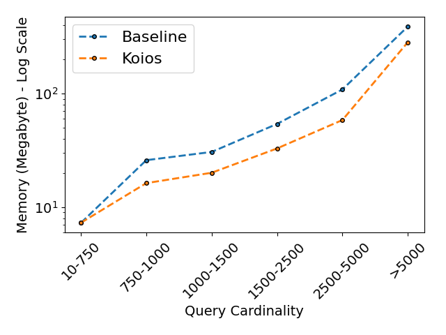
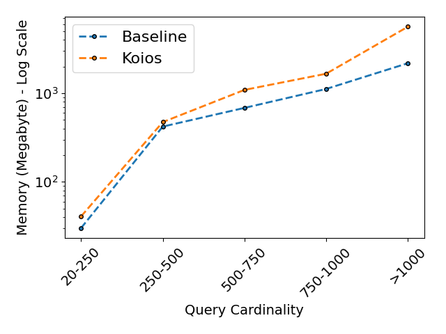
Koios is an in-memory algorithm. We report the average memory across benchmarks for all datasets in Table III. The extended version of the paper contains an in-depth analysis of Koios memory footprint. Fig. 5(d) and 6(d) show the memory footprint of Koios and the baseline for OpenData and WDC. The reported values are the average memory footprint of data structures over successful queries in each interval. Note that some data structures such as inverted index, token index, and top-$k$ lists have fixed sizes for all query intervals. To have the whole picture of the memory footprint, the numbers reported in these plots and Table III are the sum of the footprint of data structures used in the refinement phase and post-processing phase, although the data structures used in the refinement phase, except the top-$k$ LB list ($\mathcal{L}_{lb}$), are freed up at the end of the phase. Table III shows that Koios’ memory utilization is comparable to the baseline.

Effect of Query Cardinality: In Fig. 5(d) and 6(d), we observe that the memory footprint increases linearly with the query cardinality. This can be explained by the linear increase in the number of candidate sets (Tables IV and V), thus, the size of the query-dependent data structures: token stream, upper-bound buckets, lower-bound data structure, and priority queues increases as the query cardinality increases.

Comparing to Baseline: Fig. 5(d) and 6(d) show the average memory footprint of the baselines and Koios. For small and medium queries for both OpenData and WDC, the memory footprint is similar. For large queries, Koios takes up less memory for OpenData compared to WDC. This is because, the iUB-Filter prunes most of the candidate sets, hence reducing the size of the post-processing data structures. Note that for the baseline we do not have enough data for WDC on large queries as almost all queries time out.

VIII-E Quality of Results

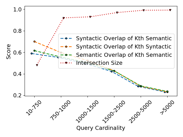
To evaluate the quality benefit of semantic overlap, we compare the top-$k$ semantic search results with the top-$k$ syntactic search results on OpenData, using the vanilla set overlap. Fig. 8 reports the scores for the $k$-th set in the top-$k$ lists. Comparing the syntactic overlap of the $k$-th set in the top-$k$ syntactic list with that of the top-$k$ semantic list, we observe that semantic overlap finds sets with lower syntactic overlap (fewer exact matching elements) but higher semantic overlap (more elements with semantic similarity). These are sets that often contain syntactically dirty elements, for example (squirrel, squirrell) and (konstantine, konstantin), or syntactically mismatching elements yet semantically similar elements, for example (Leeds, Sheffield). We also investigated the sets returned by the two searches and report the size of the intersection of results. Fig. 8 shows that semantic overlap finds sets that cannot be otherwise discovered by the vanilla overlap. In particular, for the smallest interval vanilla overlap misses $50\%$ of the results. This shows how semantic overlap can help find sets that would not be part of the top-$k$ result if only syntactic overlap was considered. Note that Koios returns an exact solution as long as the index returns exact results.

VIII-F Analysis of Parameters

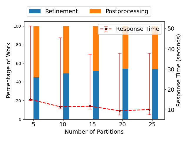
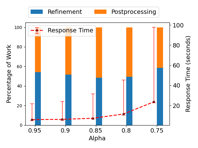
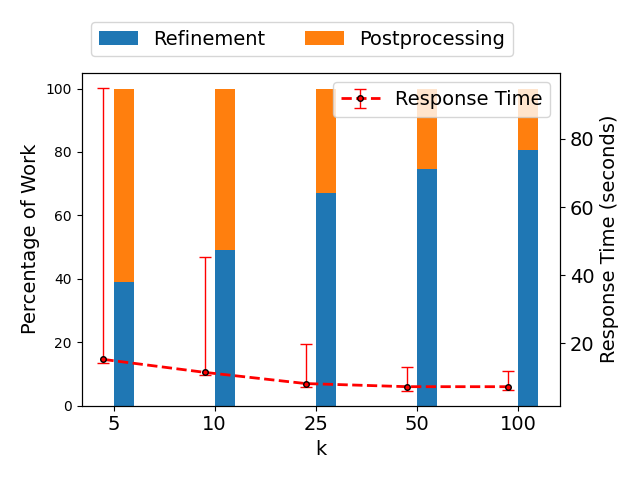
Our algorithm uses three parameters for search: 1) an element similarity threshold ($\alpha$), 2) the number of data partitions, and 3) a user-provided number of result sets ($k$). We performed an empirical study of the impact of these parameters on the response time of Koios. For this set of experiments, we choose 100 queries from the benchmark of OpenData at random. Since the set cardinality in data repositories follows a Zipfian distribution [7, 8], random sampling from benchmark intervals prevents from having a benchmark that is heavily biased to smaller query sets. Fig. 7 shows the average response time and the breakdown of the ratio of refinement and post-processing time of queries for various parameter values.

Figure 8: Comparison of vanilla and semantic overlap.

Number of Partitions: In Fig. 7(a), we fix $k=10$ and $\alpha=0.8$ and vary the number of partitions. The response time decreases as the number of partitions increases. This is because a larger number of partitions results in a smaller number of sets to process per partition. Since partitions are processed in parallel, the response time decreases with more partitions. Since sets are randomly assigned to partitions, partitions have the same expected number of sets. The top-$k$ result of all partitions are merge-sorted after all partitions finish. However, the merging cost is negligible compared to the overall runtime.

In addition to the average response time, Fig. 7(a) reports the average percentage of work in the refinement and post-processing of a partition. One interesting observation is that as the number of partitions increases, the percentage of post-processing sets becomes smaller. This is because, with a large number of partitions, more sets are considered per time unit across all partitions and $\theta_{lb}$ grows quickly. As a result, iUB-Filter has higher pruning power.

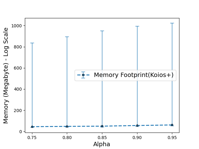
Element Similarity Threshold: In Fig. 7(b), we fix $k=10$, the number of partitions to 10, and vary the value of $\alpha$. We observe that the higher $\alpha$, the smaller the average response time for a query. A smaller $\alpha$ means more elements in the vocabulary are potentially considered for matching with element queries, and as a result, more candidate sets are considered by the algorithm. While the pruning power of refinement filters is independent of the value of $\alpha$, the cost of graph matching grows with the number of edges in a bipartite graph: smaller $\alpha$ values result in more edges in the graph and therefore higher matching time. Fig. 7(d) also shows that increasing $\alpha$ results in a slight increase in the memory footprint for Koios. This is because by increasing $\alpha$, we get a smaller token stream and a decrease in the number of candidate sets. We converge to a smaller value of $\theta_{lb}$ which results in more sets reaching post-processing; this results in larger post-processing data structures and hence the increase in the memory footprint.

Result Set Cardinality: In Fig. 7(c), we fix the number of partitions to 10 and $\alpha=0.8$ and vary the value of $k$. For a given value of $k$ in this plot, each partition runs a top-$k$ search and the final results from partitions are merged, i.e. for $k=50$, we merge ten top-$50$ lists returned from ten partitions. The observation of a decrease in average response time with the increase of $k$ is counter-intuitive since higher $k$ means lower $\theta_{lb}$ and lower pruning power of the iUB-Filter. However, the response time decreases because the average post-processing work decreases with the increase of $k$.

The response time and the post-processing work behavior can be explained by looking at the number of sets considered and those that reach post-processing. With a large $k$, since the iUB-filter prunes a lot of sets, those that reach the post-processing phase end up in the top-$k$ result, and many of them are filtered using the EM-Early-Terminated-Filter and are quickly added to the top-$k$ result.

IX Related Work

(Fuzzy) Set Similarity Search The majority of works in set similarity search take into account syntactic measures like containment and Jaccard on sets of tokens and use a threshold search [35, 9]. To avoid computing pairwise similarities of set, the common technique is to apply a filter-verification paradigm with a core step being prefix-filtering  [36, 37, 36]. PPJoin extends prefix filtering by incorporating a positional filtering technique that uses token ordering information to reduce candidate sizes even further [38]. There has also been work on partition-based search, where the goal is to partition the data to allow for faster search, for example, SSJoin and GreedyPlus [39, 40].

Table Join Search Most existing join search techniques consider equi-join and use (normalized) cardinality of the overlap of sets of attribute values as joinability measure [8, 10, 41, 7, 42, 43]. JOSIE combines filtering techniques from the set similarity search literature to solve the join search problem using vanilla overlap [8]. A common way to obtain approximate join search results is to construct an LSH index on set signatures generated using hash functions such as MinHash [20, 7, 10].

Semantic Techniques PEXESO is a threshold-based set similarity search technique based on an extension of the vanilla overlap [44]. In PEXESO, two elements are considered as “matching” if they have a similarity greater than a user-specified threshold. The set similarity is then defined as the number of elements in a query that has at least one matching element in a candidate set, normalized by the query cardinality. This implies that elements can participate in many-to-many matchings such that the vanilla overlap cannot be expressed as a special case of the proposed measure. SEMA-JOIN takes two sets of values from join columns as input and produces a predicted join relationship (many-to-one join on cell values) [14]. To do so, SEMA-JOIN finds the join relationship that maximizes the aggregate pairwise semantic correlation. Relying on a big table corpus (100M tables from the web), the statistical co-occurrence is used as a proxy for semantic correlation. The intuition is that two values can be joined semantically (e.g., GE and General Electric) if there exists significant statistical co-occurrence of these values in the same row in the corpus (row co-occurrence score). Moreover, pairs of pairs are required to be semantically compatible, i.e., they should co-occur in the same columns in the corpus (column-level co-occurrence). Finally, to join two columns, SEMA-JOIN aims at maximizing the aggregate pairwise column-level and row-level correlation. Unlike Koios , which solves the search problem of finding sets that can be joined with a query set, SEMA-JOIN finds the best way of joining column elements after discovery.

X Conclusion

We defined the semantic overlap measure. To solve the top-$k$ semantic overlap search problem, we introduced Koios, an exact and efficient filter-verification framework with powerful and cheap-to-update filters that decrease the graph-matching computation to less than $5\%$ of the candidate sets. We demonstrated that Koios has a low response time and memory footprint in experiments on four different datasets. In our future work, we plan to expand the semantic overlap to instances with many-to-1 mappings to cover noise or spelling variations within the query, for example, United States of America and United States can both be mapped to USA with equal similarity.

References

- [1] M. Hadjieleftheriou, X. Yu, N. Koudas, and D. Srivastava, “Hashed samples: selectivity estimators for set similarity selection queries,” PVLDB, vol. 1, no. 1, pp. 201–212, 2008.
- [2] P. Wang and Y. He, “Uni-detect: A unified approach to automated error detection in tables,” in SIGMOD. ACM, 2019, pp. 811–828.
- [3] M. Yu, G. Li, D. Deng, and J. Feng, “String similarity search and join: a survey,” Frontiers Comput. Sci., vol. 10, no. 3, pp. 399–417, 2016.
- [4] C. Ge, Y. Li, E. Eilebrecht, B. Chandramouli, and D. Kossmann, “Speculative distributed CSV data parsing for big data analytics,” in SIGMOD. ACM, 2019, pp. 883–899.
- [5] G. Papadakis, M. Fisichella, F. Schoger, G. Mandilaras, N. Augsten, and W. Nejdl, “Benchmarking filtering techniques for entity resolution,” in ICDE, 2023, to appear.
- [6] Y.-L. Chen, J.-J. Wei, S.-Y. Wu, and Y.-H. Hu, “A similarity-based method for retrieving documents from the sci/ssci database,” Journal of information science, vol. 32, no. 5, pp. 449–464, 2006.
- [7] E. Zhu, F. Nargesian, K. Q. Pu, and R. J. Miller, “LSH ensemble: Internet-scale domain search,” PVLDB, vol. 9, no. 12, pp. 1185–1196, 2016.
- [8] E. Zhu, D. Deng, F. Nargesian, and R. J. Miller, “JOSIE: overlap set similarity search for finding joinable tables in data lakes,” in SIGMOD, 2019, pp. 847–864.
- [9] W. Mann, N. Augsten, and P. Bouros, “An empirical evaluation of set similarity join techniques,” PVLDB, vol. 9, no. 9, pp. 636–647, 2016.
- [10] R. C. Fernandez, J. Min, D. Nava, and S. Madden, “Lazo: A cardinality-based method for coupled estimation of jaccard similarity and containment,” in ICDE, 2019, pp. 1190–1201.
- [11] J. Wang, G. Li, and J. Fe, “Fast-join: An efficient method for fuzzy token matching based string similarity join,” in ICDE, 2011, pp. 458–469.
- [12] J. Wang, G. Li, and J. Feng, “Extending string similarity join to tolerant fuzzy token matching,” ACM Trans. Database Syst., vol. 39, no. 1, pp. 7:1–7:45, 2014.
- [13] D. Deng, A. Kim, S. Madden, and M. Stonebraker, “Silkmoth: An efficient method for finding related sets with maximum matching constraints,” PVLDB, vol. 10, no. 10, pp. 1082–1093, 2017.
- [14] Y. He, K. Ganjam, and X. Chu, “SEMA-JOIN: joining semantically-related tables using big table corpora,” PVLDB, vol. 8, no. 12, pp. 1358–1369, 2015.
- [15] J. R. Edmonds and R. M. Karp, “Theoretical improvements in algorithmic efficiency for network flow problems,” J. ACM, vol. 19, no. 2, pp. 248–264, 1972.
- [16] G. Navarro, “A guided tour to approximate string matching,” ACM computing surveys (CSUR), vol. 33, no. 1, pp. 31–88, 2001.
- [17] I. F. Ilyas, G. Beskales, and M. A. Soliman, “A survey of top-k query processing techniques in relational database systems,” ACM Comput. Surv., vol. 40, no. 4, pp. 11:1–11:58, 2008.
- [18] V. V. Vazirani, Approximation algorithms. Springer, 2001.
- [19] J. Johnson, M. Douze, and H. Jégou, “Billion-scale similarity search with GPUs,” IEEE Transactions on Big Data, vol. 7, no. 3, pp. 535–547, 2019.
- [20] A. Z. Broder, “On the resemblance and containment of documents,” in SEQUENCES, B. Carpentieri, A. D. Santis, U. Vaccaro, and J. A. Storer, Eds., 1997, pp. 21–29.
- [21] P. Agrawal, A. Arasu, and R. Kaushik, “On indexing error-tolerant set containment,” in SIGMOD, A. K. Elmagarmid and D. Agrawal, Eds. ACM, 2010, pp. 927–938.
- [22] D. Deng, G. Li, J. Feng, and W. Li, “Top-k string similarity search with edit-distance constraints,” in ICDE, 2013, pp. 925–936.
- [23] J. Wang, G. Li, D. Deng, Y. Zhang, and J. Feng, “Two birds with one stone: An efficient hierarchical framework for top-k and threshold-based string similarity search,” in ICDE, 2015, pp. 519–530.
- [24] J. Munkres, “Algorithms for the assignment and transportation problems,” 1957.
- [25] Z. Galil, “Efficient algorithms for finding maximum matching in graphs,” vol. 18, no. 1, p. 23–38, 1986.
- [26] M. L. Fredman and R. E. Tarjan, “Fibonacci heaps and their uses in improved network optimization algorithms,” J. ACM, vol. 34, no. 3, pp. 596–615, 1987.
- [27] P. K. Agarwal and R. Sharathkumar, “Approximation algorithms for bipartite matching with metric and geometric costs,” in STOC, D. B. Shmoys, Ed. ACM, 2014, pp. 555–564.
- [28] A. Joulin, E. Grave, P. Bojanowski, and T. Mikolov, “Bag of tricks for efficient text classification,” in EACL, 2017, pp. 427–431.
- [29] H. Jelodar and et al, “Recommendation system based on semantic scholar mining and topic modeling on conferences publications,” Soft Computing, vol. 24, pp. 1–30, 2020.
- [30] F. Nargesian, E. Zhu, K. Q. Pu, and R. J. Miller, “Table union search on open data,” PVLDB, vol. 11, no. 7, pp. 813–825, 2018.
- [31] J. M. Banda, R. Tekumalla, G. Wang, J. Yu, T. Liu, Y. Ding, and G. Chowell, “A large-scale COVID-19 twitter chatter dataset for open scientific research - an international collaboration,” CoRR, vol. abs/2004.03688, 2020. [Online]. Available: https://arxiv.org/abs/2004.03688
- [32] O. Lehmberg, D. Ritze, R. Meusel, and C. Bizer, “A large public corpus of web tables containing time and context metadata,” in WWW, 2016, pp. 75–76.
- [33] Mcximing, “mcximing/hungarian-algorithm-cpp: A c wrapper for a hungarian algorithm implementation.” [Online]. Available: https://github.com/mcximing/hungarian-algorithm-cpp
- [34] B. Shoshany, “A C++17 thread pool for high-performance scientific computing,” CoRR, vol. abs/2105.00613, 2021.
- [35] L. Jia, L. Zhang, G. Yu, J. You, J. Ding, and M. Li, “A survey on set similarity search and join,” International Journal of Performability Engineering, vol. 14, no. 2, p. 245, 2018.
- [36] R. J. Bayardo, Y. Ma, and R. Srikant, “WWW,” C. L. Williamson, M. E. Zurko, P. F. Patel-Schneider, and P. J. Shenoy, Eds. ACM, 2007, pp. 131–140. [Online]. Available: https://doi.org/10.1145/1242572.1242591
- [37] S. Chaudhuri, V. Ganti, and R. Kaushik, “A primitive operator for similarity joins in data cleaning,” in Proceedings of the 22nd International Conference on Data Engineering, ICDE 2006, 3-8 April 2006, Atlanta, GA, USA, L. Liu, A. Reuter, K. Whang, and J. Zhang, Eds. IEEE Computer Society, 2006, p. 5. [Online]. Available: https://doi.org/10.1109/ICDE.2006.9
- [38] C. Xiao, W. Wang, X. Lin, J. X. Yu, and G. Wang, “Efficient similarity joins for near-duplicate detection,” ACM Trans. Database Syst., vol. 36, no. 3, pp. 15:1–15:41, 2011. [Online]. Available: https://doi.org/10.1145/2000824.2000825
- [39] A. Arasu, V. Ganti, and R. Kaushik, “Efficient exact set-similarity joins,” in Proceedings of the 32nd international conference on Very large data bases, 2006, pp. 918–929.
- [40] D. Deng, G. Li, H. Wen, and J. Feng, “An efficient partition based method for exact set similarity joins,” Proceedings of the VLDB Endowment, vol. 9, no. 4, pp. 360–371, 2015.
- [41] D. Deng, C. Yang, S. Shang, F. Zhu, L. Liu, and L. Shao, “Lcjoin: Set containment join via list crosscutting,” in ICDE, 2019, pp. 362–373.
- [42] A. Bogatu, A. A. A. Fernandes, N. W. Paton, and N. Konstantinou, “Dataset discovery in data lakes,” in ICDE, 2020, pp. 709–720.
- [43] S. Castelo, R. Rampin, A. S. R. Santos, A. Bessa, F. Chirigati, and J. Freire, “Auctus: A dataset search engine for data discovery and augmentation,” PVLDB, vol. 14, no. 12, pp. 2791–2794, 2021.
- [44] Y. Dong, K. Takeoka, C. Xiao, and M. Oyamada, “Efficient joinable table discovery in data lakes: A high-dimensional similarity-based approach,” in ICDE, 2021, pp. 456–467.