Résumé

This work measures how sparsity can make neural networks more robust to membership inference attacks. The obtained empirical results show that sparsity improves the privacy of the network, while preserving comparable performances on the task at hand. This empirical study completes and extends existing literature.

1 Introduction

Deep neural networks are state-of-the-art for many learning problems. In practice, it is possible to tune the parameters of a given network in order to perfectly interpolate the available data [21]. This overfitting regime is of practical interest since good performances can be obtained this way [3]. However, it comes with an increased risk in terms of privacy [14], since the network memorizes information about training data, up to the point of interpolating them. Among these information, some might be confidential. This raises the question of what information can be inferred given a black-box access to the model.

To detect an overfitting situation, an indicator is given by the ratio of the number of parameters by the number of data points available: the more parameters there are, the more the model can interpolate the data. In order to hinder the capacity of the model to overfit, and thus to store confidential information, this work studies the role of the number of nonzero parameters used. Can we find a good trade-off between model accuracy and privacy by tuning the sparsity (number of nonzero parameters) of neural networks?

Attacks such as "Membership Inference Attack" (MIA) can infer the membership of a data point to the training set [16], using only a black-box access to the targeted model. This can be problematic in case of sensitive data (medical data, etc.). Given a network, how could one reduce the risk of such attacks, while preserving its performances as much as possible?

Numerous procedures have been proposed to defend against MIAs [8]. In this work, the studied approach consists in decreasing the number of nonzero parameters used by the network in order to reduce its memorization capacity, while preserving as much as possible its accuracy.

Figure 1: Means and standard deviations of the accuracy and defense level of various sparse networks. The percentage of nonzero weights is given in blue for IMP ($*$ p$\%$), and in red for Butterfly (• p$\%$). The color emphasizes the sparsity level. The line has a slope of $-3.25$.

Related works.

The links between neural network sparsity and privacy have already been partially explored, but, to the best of our knowledge, it has not yet been shown that sparsity improves privacy without further adjustment of the training algorithm. A comparison with literature is done in section 4.

Figure 2: Experiments obey to the following pipeline: two networks are trained in the same fashion on $\mathcal{D}_{\text{train}}^{\text{target}}$ and $\mathcal{D}_{\text{train}}^{\text{shadow}}$ respectively. $\mathcal{R}^{\text{shadow}}$, $\mathcal{D}_{\text{train}}^{\text{shadow}}$ and $\mathcal{D}_{\text{test}}^{\text{shadow}}$ are then used to train a discriminator that will attack $\mathcal{R}^{\text{target}}$ by trying to infer the membership of $x$ in $\mathcal{D}_{\text{train}}^{\text{target}}$.

Contributions and results.

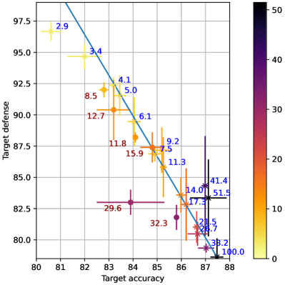
The results of the experiments in section 4 support the hypothesis that sparsity improves the defense against MIAs while maintaining comparable performances on the learning task. However, the standard deviations reported in the experiments suggest that larger scale experiments are needed before confirming this trend. Figure 1 shows that the trade-off between robustness to MIA and network accuracy is similar between unstructured sparsity, obtained by an Iterative Magnitude Pruning (IMP) [5] of the weights, and structured "butterfly" sparsity, where the weights matrices are constrained to admit some structured sparse factorization [12, 4]. To the best of our knowledge, the "butterfly" structure has not been studied before in this context. This structure achieves similar trade-offs as IMP, which is remarkable, as the structure is fixed beforehand, independently of the data. Moreover, software and hardware optimizations can be envisioned to leverage butterfly sparsity in order to implement matrix-vector multiplications in a more efficient way than it is without sparsity or with unstructured sparsity.

Experiments on CIFAR-10 show that when the percentage of nonzero weights in ResNet-20 is between $3.4\%$ and $17.3\%$, a relative loss of $p\%$ in accuracy, compared to the trained dense network , leads to a relative gain of $3.6\times p\%$ in defense against MIA, see Figure 1.

Section 2 introduces the MIAs used for the experiments. Section 3 describes the types of sparsity used to defend against MIAs. The results of the experiments are presented in section 4, with a comparison to literature.

2 MIA with a shadow model

Let $\mathcal{D}$ be a dataset and $\mathcal{D}_{\text{train}}\subset\mathcal{D}$ be a training subset. The associated membership function $m_{\mathcal{D}_{\text{train}},\mathcal{D}}$ is defined by:

$$m_{\mathcal{D}_{\text{train}},\mathcal{D}}:x\in\mathcal{D}\mapsto\left\{\begin{array}[]{cc}1&\textrm{if }x\in\mathcal{D}_{\text{train}},\\ 0&\textrm{otherwise}.\end{array}\right.$$

Given a dataset $\mathcal{D}^{\text{target}}$, and a target network $\mathcal{R}^{\text{target}}$ trained on a subset $\mathcal{D}_{\text{train}}^{\text{target}}$ of $\mathcal{D}^{\text{target}}$, a MIA consists in retrieving the associated membership function $m_{\text{target}}:=m_{\mathcal{D}_{\text{train}}^{\text{target}},\mathcal{D}^{\text{target}}}$, with only a black-box access to the function $x\mapsto\mathcal{R}^{\text{target}}(x)$. Most of the known attacks are based on an observation of the output of the $\mathcal{R}^{\text{target}}$ model, locally around $x$ [8]. In general, these attacks seek to measure the confidence of the model in its predictions made locally around $x$. If the measured confidence is high enough, then the attacker answers positively to the membership question.

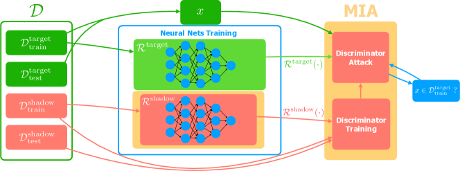
In practice, the most efficient attacks consist in training a discriminator model that makes a decision based on local information of $\mathcal{R}^{\text{target}}$ around $x$. This discriminator is trained from a shadow network [8], as explained below (see also Figure 2).

Suppose that the attacker has access to a dataset $\mathcal{D}^{\text{shadow}}$ from the same distribution as $\mathcal{D}^{\text{target}}$. It then trains its own shadow network $\mathcal{R}^{\text{shadow}}$ on a subset $\mathcal{D}_{\text{train}}^{\text{shadow}}$ of the data it owns. Ideally, $\mathcal{R}^{\text{shadow}}$ is trained under the same conditions as $\mathcal{R}^{\text{target}}$ (same architecture and same optimization algorithm). The attacker then has a tuple $(\mathcal{R}^{\text{shadow}},\mathcal{D}^{\text{shadow}},\mathcal{D}_{\text{train}}^{\text{shadow}})$ which is similar to $(\mathcal{R}^{\text{target}},\mathcal{D}^{\text{target}},\mathcal{D}_{\text{train}}^{\text{target}})$, and he knows the shadow membership function $m_{\text{shadow}}:=m_{\mathcal{D}_{\text{train}}^{\text{shadow}},\mathcal{D}^{\text{shadow}}}$.

Discriminator.

The attacker can then train a discriminator to approximate $m_{\text{shadow}}$, given a black box access to $\mathcal{R}^{\text{shadow}}$. This discriminator can then be used to approximate $m_{\text{target}}$ given a black box access to $\mathcal{R}^{\text{target}}$. The model for the discriminator can be any classical classifier (logistic regression, neural network, etc.) [8].

3 Defense and neural network pruning

Training sparse neural networks is first motivated by needs for frugality in resources (memory, inference time, training time, etc.).

Here, the following hypothesis is investigated: sparsity can limit the model’s ability to store confidential information about the data it has been trained on. A perfectly confidential network has not learned anything from its data and has no practical interest. A trade-off between confidentiality and accuracy must be made according to the task at hand. In what follows, two types of sparsity are considered.

3.1 Unstructured sparsity via IMP

In the first case, no specific structure is imposed on the set of nonzero weights. The weights that are set to zero (pruned) are selected by an iterative magnitude pruning process (IMP) [5]: (i) train a network the usual way, (ii) prune $p\%$ of the weights having the smallest magnitude, (iii) adjust the remaining weights by re-training the network (weights that have been pruned are masked and are no longer updated), then go back to (ii) until the desired level of sparsity is reached.

This procedure allows to find sparse networks with empirical good statistical properties [5, 6].

3.2 Structured butterfly sparsity

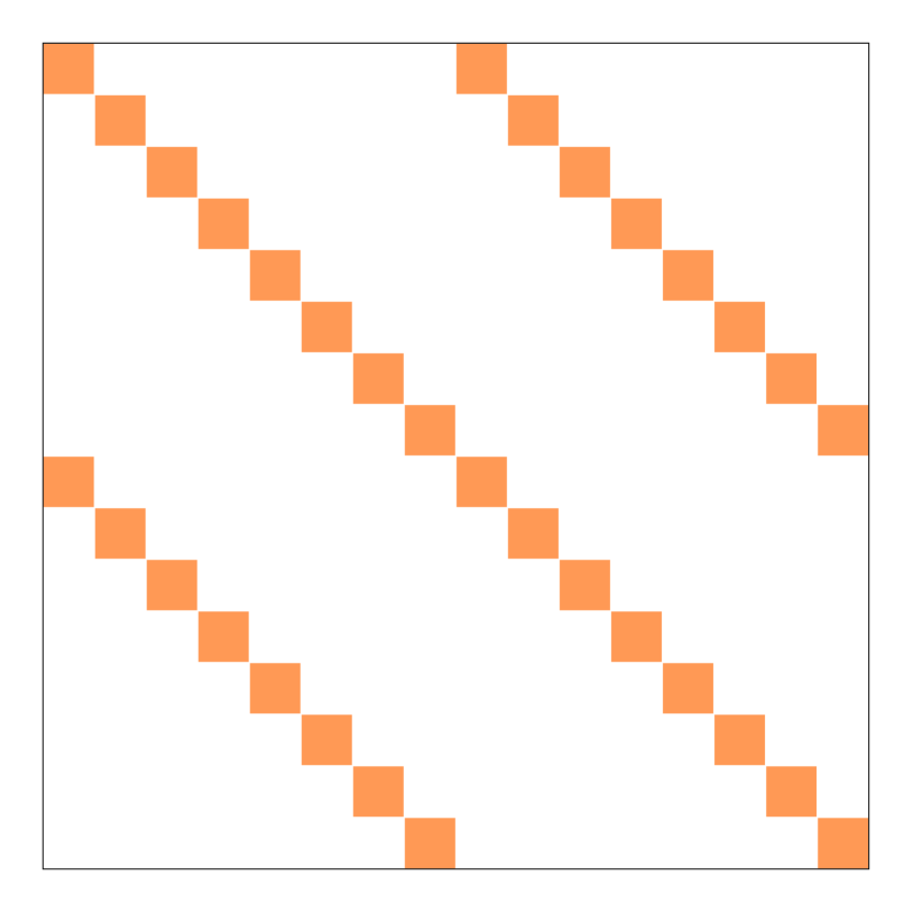
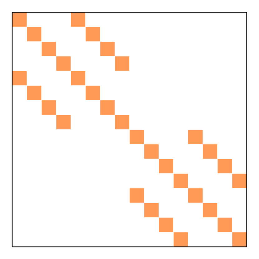
In the second case, the sparsity is structured: the weight matrices of the neural network are constrained to admit a "butterfly" factorization [11], for which the associated matrix-vector multiplication can be efficiently implemented [4]. A square matrix $\mathbf{W}$ of size $N:=2^{L}$ has a butterfly factorization if it can be written as an exact product $\mathbf{W}=\mathbf{X}^{(1)}\ldots\mathbf{X}^{(L)}$ of $L$ square factors of size $N$, where each factor satisfies the support constraint $\text{supp}(\mathbf{X}^{(\ell)})\subseteq\text{supp}(\mathbf{S}_{\textrm{bf}}^{(\ell)})$, with $\mathbf{S}_{\textrm{bf}}^{(\ell)}:=\mathbf{I}_{2^{\ell-1}}\otimes[\begin{smallmatrix}1&1\\ 1&1\end{smallmatrix}]\otimes\mathbf{I}_{N/2^{\ell}}$. See Figure 3 for an illustration. The factors have at most two nonzero entries per row and per column. Leveraging this factorization, matrix-vector multiplication has a complexity of $\mathcal{O}(N\log N)$, against $\mathcal{O}(N^{2})$ in general.

(a) $\mathbf{S}_{\mathrm{bf}}^{(1)}$

(b) $\mathbf{S}_{\mathrm{bf}}^{(2)}$

(c) $\mathbf{S}_{\mathrm{bf}}^{(3)}$

(d) $\mathbf{S}_{\mathrm{bf}}^{(4)}$

Figure 3: Supports in a butterfly factorization of size $N=16$.

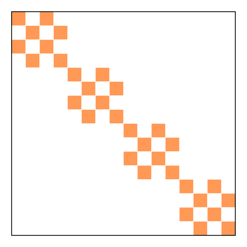
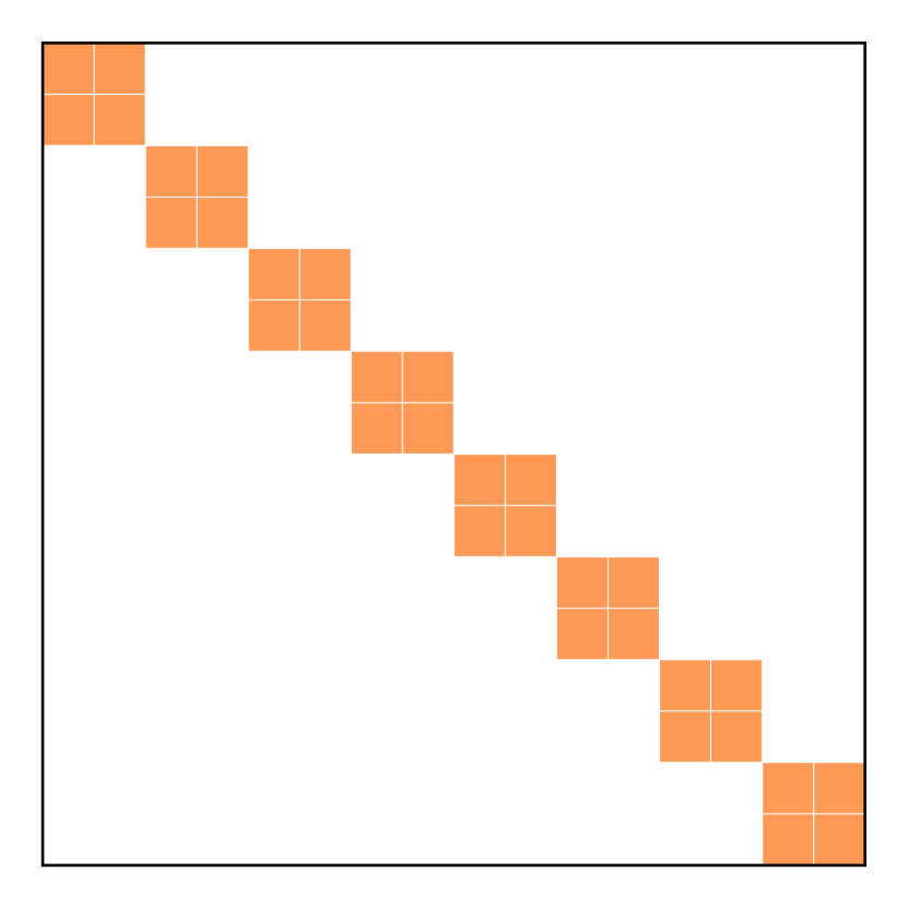
To enforce the butterfly structure in a neural network, the weight matrices $\mathbf{W}$ are parameterized as $\mathbf{W}=\mathbf{X}^{(1)}\ldots\mathbf{X}^{(L)}$, and only the nonzero coefficients of $\mathbf{X}^{(1)},\ldots,\mathbf{X}^{(L)}$ are initialized and then optimized by stochastic gradient descent.

In general, for a matrix $\mathbf{W}$ of arbitrary size, it is also possible to impose a similar structure but the definitions are more involved. We refer the reader to [12]. In the case of a convolution layer, the matrix $\mathbf{W}$ for which we impose such a structure corresponds to the concatenation of convolution kernels [12]. In our experiments, for a fixed size of $\mathbf{W}$ and a fixed number of factors $L$, the rectangular butterfly factorization is parameterized according to a monotone chain following [12]. Among all possible chains, the one with the minimal number of parameters is selected.

Butterfly networks can reach empirical performances comparable to a dense network on image classification tasks [4, 12].

4 Experimental results

All hyperparameters (including the discriminator architecture) have been determined following a grid search, averaged on three experiments to take into account randomness.

Dataset.

Experiments are performed on the CIFAR-10 dataset (60000 images $32\times 32\times 3$, 10 classes). The dataset is randomly (uniformly) partitioned into 4 subsets $\mathcal{D}_{\text{train}}^{\text{target}},\mathcal{D}_{\text{test}}^{\text{target}},\mathcal{D}_{\text{train}}^{\text{shadow}},\mathcal{D}_{\text{test}}^{\text{shadow}}$ of 15000 images, respectively used to train and test the target and shadow networks. The membership functions are defined as in section 2, with $\mathcal{D}^{\text{target}}:=\mathcal{D}_{\text{train}}^{\text{target}}\cup\mathcal{D}_{\text{test}}^{\text{target}}$ and $\mathcal{D}^{\text{shadow}}:=\mathcal{D}_{\text{train}}^{\text{shadow}}\cup\mathcal{D}_{\text{test}}^{\text{shadow}}$. For the target and shadow network, among their 15000 training data points, 1000 are randomly chosen and fixed for all our experiments as a validation set (used to tune the hyper-parameters, and for the stopping criterion).

Training of the target and shadow models.

The target and shadow networks have a ResNet-20 architecture [7] (272474 parameters). They are trained to minimize the cross-entropy loss by stochastic gradient descent (with $0.9$ momentum and no Nesterov acceleration) on their respective training sets for 300 epochs, with a batch size of 256. The dataset is augmented with random horizontal flipping and random cropping. The initial learning rate is divided by 10 after 150 and after 225 epochs. The weights of the neural networks are initialized with the standard method on Pytorch, following a uniform distribution on $(-1/\sqrt{n},1/\sqrt{n})$ where $n$ is the input dimension for a linear layer, and $n$ is $\textrm{input dimension}\times\textrm{kernel width}\times\textrm{kernel height}$ for a convolution.

Values of initial learning rate and weight decay are reported in table 1. Note that the chosen hyperparameters allow to reproduce results of [7] when using the whole 50000 training images of CIFAR-10 instead of 15000 of them as it is done for the target and shadow networks.

For IMP, 24 prunings and readjustments of the parameters are performed. Each readjustment is done with the same training procedure as above (300 epochs, etc.). Before each pruning, the weights are rewound to the values they had at the end of the epoch of maximum validation accuracy in the last $300$ epochs.

For training ResNet-20 with the butterfly structure, the original weight matrices of some convolution layers are substituted by matrices admitting a butterfly factorization, with a number $L=2$ or $3$ of factors, following a monotonic chain minimizing the number of parameters in the factorization, as described in section 3.2. The substituted layers are those of the $S=1,2$ or $3$ last segments of ResNet-20.

Table 1: Hyperparameters for the training of the target and the shadow neural networks.

Network	$\%$ of nonzero params	Initial learning rate	Weight decay
ResNet-20 dense	100 %	$0.03$	$0.005$
Butterfly ($S=1,L=2$)	32.3 %	0.3	0.0005
Butterfly ($S=1,L=3$)	29.6 %	0.3	0.0001
Butterfly ($S=2,L=2$)	15.9 %	0.3	0.0005
Butterfly ($S=2,L=3$)	12.9 %	0.1	0.001
Butterfly ($S=3,L=2$)	11.8 %	0.3	0.0005
Butterfly ($S=3,L=3$)	8.5 %	0.1	0.001
IMP with $k$ prunings	$\simeq 100\times(0.8)^{k}\%$	$0.03$	$0.005$

Discriminator training.

A discriminator takes as inputs the class $i$ of $x$, the prediction $\mathcal{R}(x)$ made by a network $\mathcal{R}$ (target or shadow), as well as $\frac{1}{\epsilon}\mathbb{E}\left(|\mathcal{R}(x)-\mathcal{R}(x+\epsilon\mathcal{N})|\right)$ ($\epsilon=0.001$ and $\mathcal{N}$, an independent centered and reduced Gaussian vector) that encodes local first order information of $\mathcal{R}$ around $x$. The expectation is estimated by averaging over 5 samples. For each pair of networks ($\mathcal{R}^{\text{target}}$,$\mathcal{R}^{\text{shadow}}$), three discriminators (perceptrons) are trained, with respectively 1, 2, 3 hidden layer(s) and 30, 30, 100 neurons on each hidden layer. The binary cross entropy is minimized with Adam for 80 epochs, without weight decay and for three different learning rates $\{0.01,0.001,0.0001\}$.

Accuracy and defense

The accuracy of a network is the percentage of data whose class is the one predicted with the highest probability by the network. The defense $D$ of a network against a discriminator is defined as $D=200-2A$ where $A$ is the accuracy of the discriminator on the membership classification task associated with the training and test data of the considered network. For example, if a discriminator has an attack accuracy $A=50+x$, then the defense is $D=100-2x$. In our case, there are as much training and testing data points for the network (target or shadow). Ideally, the discriminator should not do better than guessing randomly, having then an accuracy of $50\%$.

Results

Dense target and shadow networks achieve on average $87.5\%$ accuracy on the test set. This accuracy decreases with sparsity, see Figure 1. A gain (or loss) in defense is significant if the interval with upper (resp. lower) bound being the mean plus (resp. minus) the standard deviation is disjoint from the interval corresponding to the trained dense network. A significant gain (or loss) in defense is only observed for a proportion of nonzero weight between $0\%$ and $17.3\%$, and for $41.4\%$ and $51.5\%$. Between $3.4\%$ and $17.3\%$, a relative loss of $p\%$ in accuracy, compared to the trained dense network, leads to a relative gain of $3.6\times p\%$: $3.6\simeq\frac{|\textrm{defense}-\textrm{defense dense}|}{\textrm{defense dense}}\frac{\textrm{accuracy dense}}{|\textrm{accuracy}-\textrm{accuracy dense}|}$.

Related work on sparsity as a defense mechanism.

Experimental results from [20] suggest on the contrary that training a network with sparse regularization from IMP degrades privacy. But these results were not averaged over multiple experiments to reduce variability due to randomness. The experiments of [20] are also performed on CIFAR-10 but with a model with $40$ times as many weights as ResNet-20, and for a proportion of nonzero weights above $50\%$. Given the standard deviations observed in Figure 1 for sparsity levels above $20\%$ on ResNet-20, one should remain cautious about the interpretation of the results of [20].

[18] also showed recently that decreasing the number of parameters of a model can improve defense to MIAs. This is complementary to this article. Note however that the way the number of parameters are reduced are fundamentally different since [18] consider smaller dense networks while, here, sparse subnetworks are consider. These types of networks may not have the same privacy-accuracy trade-off.

Given a sparsity level, [19] looks for the parameters that minimize the loss function of the learning problem, penalized by the highest MIA attack accuracy achievable against these parameters. Note that this penalty term is in general not explicitly computable, and difficult to minimize. Moreover, this requires to know in advance the type of attack that targets the network, e.g., the architecture of the attacker, etc. No comparison with the non-penalized case has been proposed in [19], which makes it unclear whether this penalization is necessary to improve privacy or if sparsity without additional penalization is sufficient. In contrast, our experiments do suggest the latter. Moreover, [19] only displays the defense achieved at the sparsity level with the smallest penalized loss function. In comparison, Figure 1 shows the robustness to MIAs for a whole range of different sparsity levels.

Finally, it has been observed that enforcing sparsity during the training of neural networks with DP-SGD ("Differentially Private Stochastic Gradient Descent") [1, 2] improves the accuracy, compared to the dense network, while keeping the same guarantees of Differential Privacy (giving strong privacy guarantees) [9, 2]. However, compared to SGD, DP-SGD suffers from a performance drop and a high computational demand that is prohibitive for large-scale experiments [15, 10]. In contrast, the privacy enhancement investigated in this work comes at a lower cost (in both accuracy and resources) but does not provide any theoretical guarantee.

5 Conclusion

The results obtained support the following conjecture: sparsity is a defense mechanism against membership inference attacks, as it reduces the effectiveness of attacks with a relatively low cost on network accuracy. This is in particular the case for structured butterfly sparsity, which had not yet been investigated in this context to the best of our knowledge.

Extending the experiments to a richer class of models, datasets and attacks would support the interest of sparsity as a defense mechanism. In the future, sparsity could serve as a baseline to decrease privacy threats since it comes at a lower computational cost than methods providing strong theoretical guarantees such as DP-SGD, does not require to know the kind of attack in advance, allows for fast matrix-vector multiplication when using structured sparsity such as the butterfly structure, and, compared to penalized loss where the attacker could infer the typical behaviour of the model on training data [17], it may not lead to bias easily exploitable by an attacker.