Generalizing Neural Human Fitting to Unseen Poses With
Articulated SE(3) Equivariance

Abstract

We address the problem of fitting a parametric human body model (SMPL) to point cloud data. Optimization-based methods require careful initialization and are prone to becoming trapped in local optima. Learning-based methods address this but do not generalize well when the input pose is far from those seen during training. For rigid point clouds, remarkable generalization has been achieved by leveraging SE(3)-equivariant networks, but these methods do not work on articulated objects. In this work we extend this idea to human bodies and propose ArtEq, a novel part-based SE(3)-equivariant neural architecture for SMPL model estimation from point clouds. Specifically, we learn a part detection network by leveraging local SO(3) invariance, and regress shape and pose using articulated SE(3) shape-invariant and pose-equivariant networks, all trained end-to-end. Our novel pose regression module leverages the permutation-equivariant property of self-attention layers to preserve rotational equivariance. Experimental results show that ArtEq generalizes to poses not seen during training, outperforming state-of-the-art methods by $\sim$44% in terms of body reconstruction accuracy, without requiring an optimization refinement step. Furthermore, ArtEq is three orders of magnitude faster during inference than prior work and has 97.3% fewer parameters. The code and model are available for research purposes at https://arteq.is.tue.mpg.de.

1 Introduction

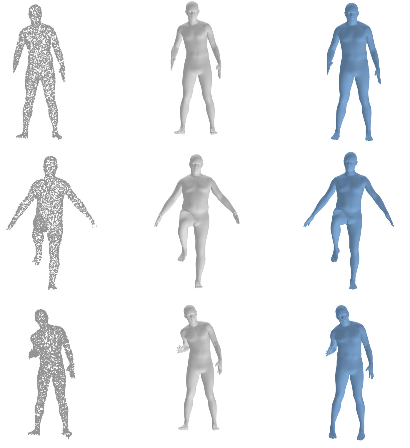
The three-dimensional (3D) capture of humans in varied poses is increasingly common and has many applications including synthetic data generation [35], human health analysis [57], apparel design and sizing [51], and avatar creation [10, 36, 50, 55]. Existing 3D body scanners output unordered point clouds, which are not immediately useful for the above applications. Consequently, the first step in processing such data is to register it; that is, to transform it into a canonical and consistent 3D representation such as a mesh with a fixed topology. For human bodies, this is typically done by first fitting a parametric model like SMPL [31] to the data; see Figure 1. Such a process should be efficient and general; that is, it should work for any input body scan, no matter the complexity of the pose. However, this is challenging given the articulated structure of the body and the high degree of variation in shape and pose.

Traditional optimization-based methods for fitting bodies to point clouds [2, 7, 8, 25, 21] are usually based on ICP [11] or its variants [2, 38, 62]. These approaches can recover accurate results even for complex poses, but require a good initialization, are computationally expensive, and may require significant manual input. Inspired by progress made in neural architectures for rigid 3D point clouds [41, 42, 59, 48], learning-based approaches have been proposed to solve the registration task. Previous approaches directly regress model parameters [24, 54, 30], intermediate representations such as correspondences [5, 6], or mesh vertex positions [19, 39, 60]. While less accurate than optimization, they can be used to initialize an optimization-based refinement step for improved accuracy [15].

A major limitation of learning-based approaches, as reported in several recent papers [5, 6, 54], is their poor generalization to body poses that lie outside the training distribution. To understand why, let us first consider how a parametric model such as SMPL explains the input point cloud. Given the shape parameters, the model first generates the overall body structure by deforming a template mesh in a canonical pose. Pose-dependent offsets are then added to the mesh. This deformed mesh then undergoes an articulated transformation that poses the body parts rigidly, and linear blend skinning is applied to smooth the result. Therefore, the observed point cloud is modeled as a combination of a canonical body shape, a part-based articulated model, and non-rigid pose-corrective deformations. When training networks to fit SMPL to point clouds, the networks are tasked with capturing the joint distribution of canonical shape and pose deformation, entangling these factors while learning a prior over plausible body shape and pose. This data-dependent prior is useful to infer new, in-distribution samples, but becomes a limitation when it comes to poses that are far from the training set. Ideally, if the networks were designed to be equivariant to articulated body pose transformations, then unseen body poses at test time would not be a problem.

A function (network) $f:V\to W$ is said to be equivariant with respect to a group $\mathcal{G}$ if, for any transformation $\mathcal{T}\in\mathcal{G},f(\mathcal{T}\mathbf{X})=\mathcal{T}f(\mathbf{X})$, $\mathbf{X}\in V$. This property can aid in generalization since it allows one to train with only “canonical” inputs $f(\mathbf{X})$, while generalizing, by design, to any transformation of the group $\mathcal{T}f(\mathbf{X})$. For example, SE(3)-equivariant networks have been used to address the out-of-distribution (OOD) generalization problem in rigid point cloud tasks, see for example [16, 40, 9]. However, extending this to the human body is far from straightforward, due to 1) its high degree of articulation, 2) the entanglement of pose and shape, and 3) deformations that are only approximately rigid.

In this work we introduce ArtEq, a new neural method that regresses SMPL shape and pose parameters from a point cloud. Our key insight is that non-rigid deformations of the human body can be largely approximated as part-based, articulated, rigid SE(3) transformations, and that good generalization requires a proper integration of equi-/in-variant properties into the network. With this in mind, we propose a novel equi-/in-variant architecture design based on the discretized SE(3)-equivariant framework [9, 12]. We learn a part detection network by leveraging local SO(3) invariance and regress shape and pose by proposing articulated SE(3) shape-invariant and pose-equivariant networks, all trained in an end-to-end manner. We further propose a novel pose regression module that leverages the permutation-equivariant property of self-attention layers to preserve rotational equivariance. Finally, to facilitate generalization to unseen poses, we cast pose regression as a weight prediction task, in which the predicted weights are used to calculate a weighted average over each of the discretized SO(3) rotations to obtain the final result.

Our empirical studies demonstrate the importance of introducing SE(3) equi-/in-variance for the task of SMPL pose and shape estimation from point cloud data. For out-of-distribution data, we show significant improvement over competing methods [5, 6, 54] in terms of part segmentation, as well as accuracy in pose and shape estimation, even when others are trained with SO(3) data augmentation. Notably, we outperform methods that require an optimization step, while ArtEq is purely regression-based. Our method also shows strong performance for in-distribution samples, surpassing all previous (optimization-based) methods although it only uses regression. Finally, we demonstrate how employing the right symmetries can lead to a lightweight network that is more than thirty times smaller than prior models, as well as a thousand times faster at inference time, making it easy to deploy in real-world scenarios.

In summary, we make the following contributions: (1) We propose a new framework for human shape and pose estimation from point clouds that integrates SE(3)-equi-/in-variant properties into the network architecture. (2) We propose a novel SE(3)-equivariant pose regression module that combines SE(3) discretization with the permutation-equivariant property of self-attention layers. (3) We show state-of-the-art performance on common benchmarks and datasets based on only regression, particularly for out-of-distribution poses. Additionally, our framework results in a much lighter model that performs three orders of magnitude faster than competitors at inference time. Our code and pre-trained models are available at https://arteq.is.tue.mpg.de.

2 Related Work

Human Body Registration From Point Clouds

Classic approaches for body registration typically deform a template mesh or a parametric model using some variant of the ICP [11] algorithm [2, 38, 62], often with additional cues such as color patterns [7, 8] or markers [37, 2, 3]. These optimization-based methods can produce accurate results for complex poses when properly initialized, but are prone to getting stuck in local minima when not, can be slow to generate results, and are not fully automatic.

Learning-based approaches have gained popularity, largely due to the development of effective neural networks for point cloud processing such as PointNet [41, 42], DeepSets [59], and KPConv [48]. These are trained to produce either a good initialization for a subsequent optimization process [5, 19, 54] or as end-to-end systems that directly compute either a mesh [39, 53, 60] or the parameters of a human body model [24, 6, 60, 30]. Our method falls into the last category.

Model-based registration reduces the task to estimating pose and/or shape parameters of a human body model such as SMPL [32]. It has been noted that it is difficult to directly regress the parameters of a SMPL model from point clouds [24, 5, 6, 53, 54]. To circumvent this, current approaches go through intermediate representations such as joint-level features [24, 30] and correspondence maps [6, 54], or resort to temporal data and motion models [23]. Similar to this work, part-based segmentation has been used as an additional cue for registration [28, 5, 6, 54]. Closely related to our work, PTF [54] isolates each segmented part and regresses a local transformation from input space to canonical space, from which pose parameters are obtained via least-squares fitting.

Without explicitly considering rotational symmetries, previous methods struggle to generalize to poses unseen during training, which limits their applicability. To the best of our knowledge, ours is the first work on model-based human point cloud registration specifically designed to correctly and efficiently handle out-of-distribution poses.

Equivariant Learning on Point Clouds

The success of CNNs is largely attributed to the translational equivariance property of such networks. Consequently, there has been an increasing interest in making neural networks invariant or equivariant to other symmetry groups [59, 41, 27, 46, 14, 56, 17, 9, 18, 16, 44, 4, 13, 40]. Of particular interest for point cloud processing is the SE(3) equivariance group. Methods for achieving SE(3) equivariance include: Vector Neurons [16], which employ tensor features and accordingly designed linear/non-linear equivariant layers; Tensor Field Networks (TFN) [49] and SE3-transformers [18], which build on top of the SO(3) representation theory with spherical harmonics and Clebsch-Gordan coefficients; methods that make use of group averaging theory [40, 4, 43]; and methods that employ a discretization of the SO(3) space to achieve equivariance [12, 9]. Within this last group, EPN [9] uses separable discrete convolutions (SPConv) that split the 6D SE(3) convolutions into SO(3) and translational parts, improving computational efficiency. Here, we employ the discrete SO(3) framework along with SPConv layers, as it allows us to leverage the discretized space to simplify the problem of pose regression, and has been noted by previous work to be highly effective [29].

In the case of rigid objects, SE(3)/SO(3)-equivariant networks have been applied to several tasks including classification and retrieval [17, 9], segmentation [16, 33], registration [52, 61], object manipulation [45], normal estimation [40], and pose estimation/canonicalisation [29, 47]. Also for rigid objects, disentanglement of shape and pose has been considered by some of these works, such as [26, 29]. To our knowledge, the only method that explores piece-wise equivariance for articulated objects is [40]. However, this is done in the context of shape-space learning, which takes as input already registered meshes with ground-truth part segmentation information. Our work, on the other hand, takes as input unordered and unevenly sampled point clouds, for which the parts are unknown.

3 Preliminaries

3.1 Discretized SE(3) Equivariance

Figure 2: A rotation acting in continuous space is equivalent to a permutation acting in the discretized rotation space (in a particular order). We exploit this property to design our architecture based on self-attention layers, while maintaining SO(3) equivariance.

Figure 3: Overview of ArtEq. We first obtain point-wise equivariant features using a small equivariant point network [9], which provides a $C$-dimensional feature vector per point and per-group element (i.e. the $60$ rotational symmetries of the icosahedron). We then convert these into point-wise invariant features by pooling over the rotation group to obtain a part segmentation of the point cloud. Using the segmentation, we softly aggregate the point-wise features into part-based equivariant features. A self-attention layer processes these in an efficient manner while preserving equivariance. We cast pose regression as a weight prediction task by predicting the weights necessary to perform a weighted average over each rotation element. Finally, we transform the part-based features into invariant ones to obtain an estimate of the shape.

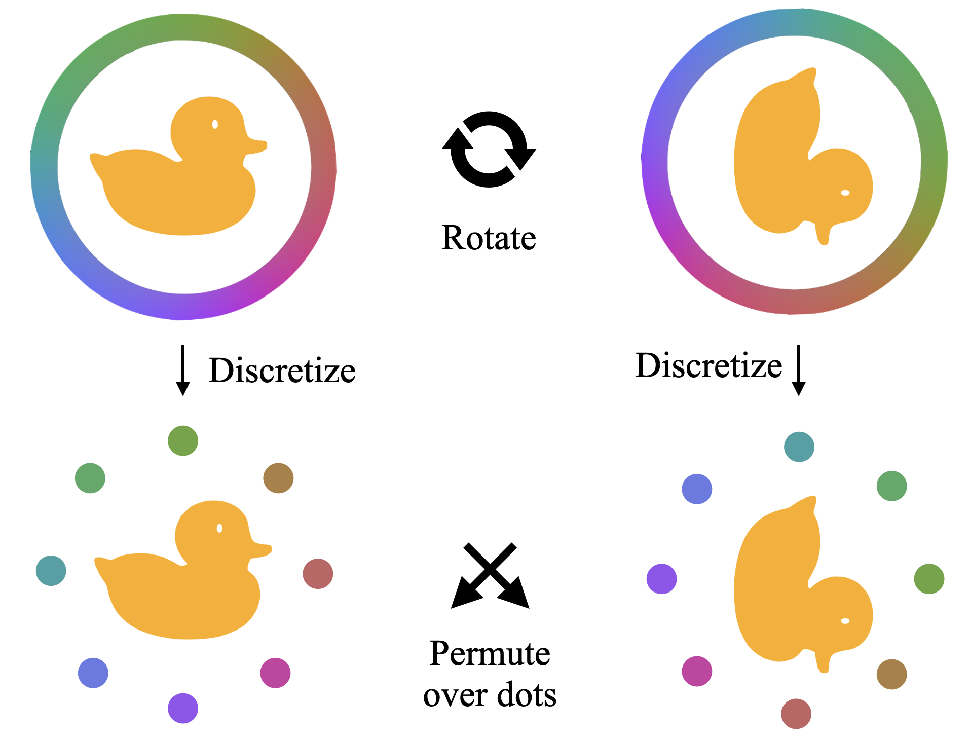
Gauge-equivariant neural networks were proposed by Cohen et al. [12] as a way to extend the idea of 2D convolutions to the manifold domain. Intuitively, instead of shifting a convolutional kernel through an image for translational equivariance, gauge-equivariant networks “shift” a kernel through all possible tangent frames for equivariance to gauge symmetries. Since this process is very computationally expensive, [12] proposed to discretize the SO(3) space with the icosahedron, which is the largest regular polyhedron, exhibiting 60 rotational symmetries. This has been further extended to operate on point clouds and the SE(3) space by EPN [9], which introduces separable convolutional layers (SPConv) to independently convolve the rotational and translational parts.

Formally, the SO(3) space can be discretized by a rotation group $\mathcal{G}$ of size $\lvert\mathcal{G}\rvert=60$, where each group element $\mathbf{g}_{j}$ represents a rotation $\mathcal{R}(\mathbf{g}_{j})$ in the icosahedral rotation group. As shown in Figure 2, a rotation acting on a continuous equivariant feature is equivalent to a permutation acting in the discretized space, where the rotation group is permuted in a specific order. This builds a connection between a rotation in a continuous space and a permutation in a discrete space. In this paper, following [12, 9], we use the rotation group $\mathcal{G}$ and the permutation operator to approximate the SO(3) space and the rotation operator.

3.2 SMPL Body Model

SMPL [31] is a statistical human body model that maps shape $\beta\in{}^{10}$ and pose $\theta\in{}^{K\times 3}$ parameters to mesh vertices $\mathbf{V}\in{}^{6890\times 3}$, where $K$ is the number of articulated joints (here $K=22$), and $\theta$ contains the relative rotation of each joint plus the root joint w.r.t. the parent in the kinematic tree, in axis-angle representation. The model uses PCA to account for variations in body shape, and Linear Blend Skinning (LBS), $W(\cdot)$, to pose the mesh.

A rest-pose mesh is first produced by

$$\mathbf{T}(\boldsymbol{\beta},\boldsymbol{\theta})=\mathbf{\bar{T}}+B_{S}(\boldsymbol{\beta})+B_{P}(\boldsymbol{\theta}),$$ (1)

where $\mathbf{\bar{T}}\in{}^{6890\times 3}$ is the template mesh, $B_{S}(\beta)$ is the linear transformation from shape parameters $\boldsymbol{\beta}$ to shape displacements, and $B_{P}(\boldsymbol{\theta})$ is the linear transformation from pose parameters to blendshape correctives that account for soft-tissue deformations due to pose. Next, joint locations are obtained for the rest-pose mesh via the linear joint regressor $J(\boldsymbol{\beta}):{}^{{\left|\boldsymbol{\beta}\right|}}\to{}^{66},J(\boldsymbol{\beta})=\{t_{1},\dots,t_{22};t_{i}\in{}^{3}\}$. Finally, SMPL applies LBS using skinning weights $\mathcal{W}$ over the rest-pose mesh to obtain the output vertices:

$$M(\boldsymbol{\beta},\boldsymbol{\theta})=W(\mathbf{T}(\boldsymbol{\beta},\boldsymbol{\theta}),J(\boldsymbol{\beta}),\boldsymbol{\theta},\mathcal{W}).$$ (2)

4 Method

Given an input point cloud $\mathbf{X}=\{\mathbf{x}_{i}\in{}^{3}\}_{N}$ of size $N$ representing a human body, the goal of this work is to regress the SMPL [31] shape $\boldsymbol{\beta}$ and pose $\boldsymbol{\theta}$ parameters that best explain the observations for any given pose, including out-of-distribution ones. Inspired by the progress in rigid SE(3)-equivariant networks [4, 9, 29], we develop an architecture that extracts part-based SE(3)- invariant/equivariant features to disentangle shape, pose, and body parts.

There are key differences between rigid objects and human bodies. First, bodies have a highly articulated structure, with different body parts undergoing various SE(3) transformations according to the kinematic tree. Therefore, global SE(3)-equivariant features cannot be directly employed, requiring, instead, local feature extraction and aggregation along with part-based semantic guidance. Second, most of the human body parts are approximately cylindrical in shape, such as the torso, legs, and arms. Cylindrical shapes have a rotational symmetry, resulting in ambiguities when recovering the pose. This is a known problem in the rigid pose estimation field [22], and cannot be resolved without external information. For human bodies, however, we can use non-ambiguous parts to help disambiguate the other ones, as we will show later. Third, when varying body poses the Euclidean neighborhood of a point might not always correspond to the geodesic neighborhood, particularly with poses that are close to self-contact. This is a problem when using point convolutional networks (such as the one developed here) since the kernel has a ball-shaped receptive field that might convolve far-away body points (i.e., close in Euclidean space but far in geodesic space), resulting in incorrect estimates.

To address this we introduce ArtEq, a part-based SE(3)-equivariant framework for human point clouds that processes articulated bodies via four modules: (1) shared locally equivariant feature extraction (Sec. 4.1), (2) part segmentation network (Sec. 4.2), (3) pose estimation network (Sec. 4.3.2) and (4) shape estimation network (Sec. 4.3.3). An overview of our method can be found in Figure 3, and we elaborate each of these in the following.

4.1 Locally Equivariant Feature Extractor

The first step of our pipeline is to obtain local per-point SO(3)-equivariant features that can be used by the subsequent modules. To this end, we train a network that takes as input the point cloud $\mathbf{X}$ and a rotation group $\mathcal{G}$ with $\lvert\mathcal{G}\rvert=M$ elements, and returns a feature tensor $\mathcal{F}\in{}^{N\times M\times C}$, comprising a feature vector of size $C$ for each of the $N$ points and each of the $M$ group elements.

Key to our design is the ability to capture local SO(3)-equivariant features via limiting the point convolution network’s effective receptive field. As mentioned earlier, human body parts that come close to each other are problematic, since the convolutional kernels might incorporate points that are geodesically distant (e.g., an arm that is almost touching a leg). This, in turn, results in reduced performance when body parts are close to each other in Euclidean space. To mitigate this, we employ a small kernel size for the SPConv layer and reduce the number of layers to only two, such that each point-wise feature in $\mathcal{F}\in{}^{N\times M\times C}$ is calculated using only a small neighboring patch.

4.2 Part Segmentation via Local SO(3) Invariance

To obtain part-based equivariance, the first step is to segment the point cloud into body parts. To achieve this while generalizing to OOD poses, we initially obtain a locally SO(3)-invariant feature by average pooling $\mathcal{F}$ over the rotation group dimension ($M$), aggregating the information from all group elements:

$$\overline{\mathcal{F}}(\mathbf{x}_{i})=\sigma\left(\{\mathcal{F}(\mathbf{x}_{i},\mathbf{g}_{1}),\mathcal{F}(\mathbf{x}_{i},\mathbf{g}_{2}),\dots,\mathcal{F}(\mathbf{x}_{i},\mathbf{g}_{M})\}\right),$$ (3)

where $\sigma$ is an aggregation function (here we use mean pooling), and $\overline{\mathcal{F}}\in\mathbb{R}^{N\times C}$ are the per-point SO(3)-invariant features that encode intrinsic geometry information. To efficiently segment the point cloud we adopt a PointNet architecture [41] with skip connections, which takes as input the invariant local feature $\overline{\mathcal{F}}(\mathbf{x}_{i})$ and outputs a vector $\alpha\in{}^{N\times 22}$, with $\alpha(\mathbf{x}_{i},\mathbf{p}_{k})$ representing the probability of point $\mathbf{x}_{i}$ belonging to body part $\mathbf{p}_{k}$. Note that PointNet is based on set operators such as pooling and point-wise convolution, and hence preserves SO(3) invariance.

4.3 Pose and Shape Estimation via Attentive SE(3) Equivariance

To disentangle pose and shape while maintaining OOD generalization we need to consider the correct symmetries for each task: part-based SE(3) equivariance for pose and part-based SE(3) invariance for shape. We explain here how to process the previously obtained part segmentation and local SO(3)-equivariant features to estimate part-based equivariant features, which are used to compute the final SMPL pose $\boldsymbol{\theta}$ and shape $\beta$ parameters.

4.3.1 Extracting Part-Based Features

The feature tensor $\mathcal{F}$ operates at the level of points. To obtain features that are useful for the part-level task of pose and shape regression, we aggregate $\mathcal{F}$ into part-based equivariant features $\mathcal{H}\in{}^{K\times M\times C}$.

A naïve solution is to simply select the points with maximum probability for a part, and average their features to obtain a unique equivariant feature of size $M\times C$ for each body part $\mathbf{p}_{k}$. However, (1) hard selection based on the argmax operation is not differentiable, and (2) points in the transition of two adjacent parts are ambiguous and can be hard to correctly select. Instead, we propose to use a soft aggregation by performing a weighted average of the equivariant features of all the points, weighted by the probability computed by the segmentation network:

$$\mathcal{H}(\mathbf{p}_{k},\mathbf{g}_{j})=\sum_{i}^{N}\alpha(\mathbf{x}_{i},\mathbf{p}_{k})\mathcal{F}(\mathbf{x}_{i},\mathbf{g}_{j}),$$ (4)

where $\mathcal{H}\in\mathbb{R}^{K\times M\times C}$ is a per-part SO(3)-equivariant feature, and $K$ is the number of body parts ($K=22$ in the case of SMPL). Similar to Equation 3 in Section 4.2, we extract the part-level SO(3)-invariant feature by aggregating the equivariant features:

$$\overline{\mathcal{H}}(\mathbf{p}_{k})=\sigma\left(\{\mathcal{H}(\mathbf{p}_{k},\mathbf{g}_{1}),\mathcal{H}(\mathbf{p}_{k},\mathbf{g}_{2}),\dots,\mathcal{H}(\mathbf{p}_{k},\mathbf{g}_{M})\}\right),$$ (5)

where $\overline{\mathcal{H}}(\mathbf{p}_{k})\in\mathbb{R}^{K\times C}$ is the per-part SO(3)-invariant feature.

4.3.2 Pose Estimation

Pose Representation

SMPL pose parameters are defined relative to their parent in the kinematic tree. However, local rotations are problematic for equivariant features, since these are defined in a global coordinate system. We estimate instead global rotation matrices that represent the rigid transformation from the part in canonical pose to the part in the current pose, from which we can recover the local rotation matrix $\boldsymbol{\theta}_{k}$ by $\boldsymbol{\theta}_{k}=\hat{\mathcal{R}}_{k}\cdot\boldsymbol{\theta}_{parent(k)}^{T}$, where $\hat{\mathcal{R}}_{k}$ is the estimated global rotation matrix, and $\boldsymbol{\theta}_{parent(k)}$ the accumulated rotation matrix of the parent.

Attentive SE(3) Equivariance

To obtain the part rotation matrices $\hat{\mathcal{R}}_{k}$, we need a function that transforms the part feature vector $\mathcal{H}(\mathbf{p}_{k})$ into a suitable representation of $\hat{\mathcal{R}}_{k}$. This function is required to preserve the equivariance by construction; if it does not (e.g., if we employ a standard MLP), the network must observe the point cloud in all possible poses to be capable of regressing arbitrary rotations. While we could, in principle, extend the network by concatenating more SPConv layers, this results in larger receptive fields, which are harmful in our particular scenario, and results in longer computation times. Instead, we can make use of the fact that rotational equivariance in continuous space is equivalent to permutation equivariance in discrete space (see [9, 13] and Section 3). Thanks to this, self-attention over group elements is an efficient alternative for preserving rotational equivariance, and we can use it to extract relationships (e.g., relative importance) among the elements of $\mathcal{G}$. Hence, we pair our initial SPConv layers with self-attention layers for efficient SE(3)-equivariant processing.

Pose Regression as Group Element Weight Prediction

Given the set of $M$ group element features, $\mathcal{H}\in{}^{K\times M\times C}$, we now need to regress a rotation for each body part. Here, we can make use of the fact that each group element feature is associated with a group element $\mathbf{g}_{j}$ (which is a rotation in the discretized SO(3) group – see Section 3.1). With this, we can regard the pose regression task as a probabilistic/weighted aggregation of the group element rotations. Specifically, we use the part-based group element features $\mathcal{H}(\mathbf{p}_{k},\mathbf{g}_{j})$ to regress one weight for each of the $M$ group elements. The final pose is calculated as the weighted chordal L2 mean [20] of the group elements with the predicted weights. Since these are predicted by self-attention layers, we can ensure that 1) rotational (permutation) equivariance is preserved and 2) the correlations between the $M$ group element features are being captured. The part-wise rotations can now be regarded as a weighted interpolation between the discrete $M$ group elements, without losing the equivariance of the group element features.

Addressing the Cylindrical Rotational Symmetry

For human bodies, we need to take into account the fact that many parts are of roughly cylindrical shape, resulting in a rotational ambiguity. However, we can leverage the fact that pairs of neighboring parts are less prone to this ambiguity. Imagine an upper leg and lower leg with a bent knee between them. Each body part on its own suffers from rotational ambiguity, but the bent knee means that the complex of both limbs has no such ambiguity. With this in mind, we condition the pose-estimation network on both a part’s feature and the feature of its parent; that is, we concatenate $\mathcal{H}(\mathbf{p}_{k})$ with the parent feature: $[\mathcal{H}(\mathbf{p}_{k})||\mathcal{H}(\mathbf{p}_{parent(k)})]$, before processing with the self-attention layers. We concatenate the root joint with itself for completeness. Experimentally, we find that this helps improve accuracy (Table 2).

4.3.3 Shape Estimation

Finally, to properly explain the observed point cloud we need to estimate the shape parameters $\boldsymbol{\beta}$ in a way that is part-wise-invariant to pose transformations. To this end, we transform $\mathcal{H}$ into a part-invariant feature by mean pooling over the group element dimension $M$, resulting in a feature matrix $\bar{\mathcal{H}}\in{}^{K\times C}$, as explained in Section 4.3.1. This feature is further processed by a few self-attention layers that capture the correlation across different body parts. The output is then flattened and fed into an MLP to produce the final $\boldsymbol{\beta}$ parameters.

4.4 Model Instance and Training

Thanks to the additional symmetry information, equivariant networks have been shown to be efficient in terms of model size and data requirements [12]. We leverage this and instantiate our framework with a minimally sized ArtEq architecture, with only two layers of SPConv that output a feature tensor with channel size $C$ = 64; two multi-head self attention (MHSA) layers for pose regression (eight heads with 64-dim embedding); and one similar MHSA for shape regression. This results in a model that is significantly smaller than competing models [54], while still delivering superior performance, as we will see in the next section.

We train the framework in a supervised manner in two stages. In a first stage, we train the part segmentation network and use ground-truth part segmentation to perform the part-level feature aggregation, while all modules are simultaneously and independently trained. In the second stage, we use the predictions from the part segmentation network for part-level feature aggregation and train the full pipeline end-to-end. Training objectives and additional details can be found in the Sup. Mat.

5 Results

In the following we show qualitative and quantitative results for ArtEq, both for in-distribution (ID) and out-of-distribution (OOD) data, and we compare with state-of-the-art methods IP-Net [5], LoopReg [6], and PTF [54]. We explain our evaluation protocol in Section 5.1, evaluate our SE(3)-invariant segmentation network in Section 5.2, and show quantitative and qualitative performance for SMPL-parameter estimation in Section 5.3. Finally, we compare performance time and model size in Section 5.4.

Method	Aug.	OOD	ID
IP-Net [5]		29.0	30.5
IP-Net [5]	$\checkmark$	86.7	91.2
LoopReg [6]	$\checkmark$	60.6	66.1
PTF [54]		8.5	10.3
PTF [54]	$\checkmark$	80.3	88.1
Ours (nc)		91.7	96.2
Ours (nc)	$\checkmark$	93.8	96.2
Ours		92.6	96.3
Ours	$\checkmark$	94.1	96.2

Table 1: Part segmentation accuracy compared to SOTA methods, in terms of percentage of correct predictions, for out-of-distribution (OOD) and in-distribution (ID) datasets. We show results with and without SO(3) data augmentation (“Aug.”), and we show our model with and without parent feature conditioning (“nc”) (Sec. 4.3.2). Best result in bold, second best underlined.

Figure 4: Qualitative results for part segmentation. Each pair of bodies shows ground-truth (left) and our result (right).

5.1 Evaluation Protocol

Datasets. We train our network using the DFAUST [8] subset of the AMASS dataset [34], which contains 100 sequences of 10 subjects with diverse body shapes. We follow the train-test split used in [10, 4] and we crop the test sequences to the middle 50% of frames, subsampling every 5 frames. We sample 5000 non-uniform points across the surface with random on-surface displacements. For ID testing we use the test split of DFAUST [8]. For OOD testing we use the PosePrior subset [1] of AMASS, which contains challenging poses that are far from those performed in DFAUST.

Metrics. The focus of this work is robustness to OOD poses, and hence we employ metrics previously proposed for this goal [10]. Specifically, for SMPL estimation we measure (1) vertex-to-vertex error (V2V) in cm and (2) joint position error (MPJPE) in cm, which are standard in the human pose community and capture the effect of errors in rotation on the final body, propagated through the kinematic tree while taking into account the predicted shape. For body part correspondence estimation, we test accuracy of part segmentation as the percentage of correct assignments. Note that a high V2V error and MPJPE, or a low part segmentation accuracy suggests a lack of robustness to outliers (OOD poses).

Comparisons. We compare our method with state-of-the-art learning-based methods that obtain SMPL parameters from point clouds [5, 6, 54]. IP-Net [5] predicts dense correspondences to the SMPL mesh, which are then used within an ICP-like optimization that recovers SMPL shape and pose parameters. LoopReg [6] extends this idea by including the SMPL optimization step within the training process of the network. PTF [54] segments body parts and regresses local transformations for each, from which pose parameters are obtained via least-squares fitting. Since all of these methods require part segmentation, we also compare our segmentation results with them. Note that IP-Net and LoopReg predict segmentation for 14 parts, while PTF and our method segment the point cloud into 24 parts, which is a harder task. For LoopReg we use their publicly available model trained on minimal clothing data, while the rest of the networks are trained using publicly available code. All methods, including ours, are trained for 15 epochs on the DFAUST train split. Note that all competitors depend on a test-time optimization step, while our results are solely based on regression.

SO(3) Data Augmentation. An alternative to SE(3) equivariant learning is to explicitly perform data augmentation. While augmenting articulated body poses is not always feasible one can easily perform global SO(3) augmentation by randomly rotating the root joint. In fact, this is already implemented by prior work, including the methods considered here. For this reason, we compare against these methods both with and without global SO(3) data augmentation. Our method, being an equivariant method, does not require augmentation to achieve good OOD generalization. However, this is still useful since it helps the network bridge the gap between the discretized SO(3) group and the continuous SO(3) group, and hence we too evaluate both with and without SO(3) augmentation.

5.2 Part Segmentation

We begin by evaluating our part segmentation network. Both for us and for competing methods, this is an important step in the pipeline that determines the quality of the final results. Since the output of this step comes directly from the networks, initial errors cannot be masked by an optimization step as it is with the SMPL estimations (see next section). We use this task to more clearly evaluate the impact of equivariant learning.

Quantitative results can be found in Table 1. Our method outperforms the competitors both for ID and OOD datasets by a large margin. Without data augmentation, IP-Net and particularly PTF perform very poorly in both cases, suggesting a fundamental limitation with respect to generalization of these methods. Our approach, on the other hand, shows superior performance over all methods both with and without data augmentation. Additionally, we observe that conditioning on the parent feature (Sec. 4.3.2) can further boost the segmentation accuracy. We show qualitative results for our method in Figure 4 and qualitative results for competing methods in the supplementary material.

Figure 5: Qualitative results for out-of-distribution poses. From left to right: (a) input point cloud, (b) ground-truth SMPL mesh, (c) our results, (d) IP-Net [5], (e) PTF [54], and (f) LoopReg [6].

Method	Aug.	OOD		ID
		V2V $\downarrow$	MPJPE $\downarrow$	V2V $\downarrow$	MPJPE $\downarrow$
IP-Net		41.58	46.99	38.55	43.41
IP-Net	$\checkmark$	7.57	9.41	5.98	6.42
LoopReg	$\checkmark$	29.08	34.09	7.57	9.17
PTF		61.42	68.43	56.35	60.98
PTF	$\checkmark$	6.42	7.56	3.05	3.53
Ours (nc)		5.41	5.91	0.95	1.04
Ours (nc)	$\checkmark$	4.17	4.61	0.95	1.03
Ours		4.73	5.51	1.13	1.48
Ours	$\checkmark$	3.62	4.23	0.98	1.26

Table 2: SMPL estimation results compared to state-of-the-art methods, with and without SO(3) augmentation (“Aug.”) for out-of-distribution (OOD) and in-distribution (ID) datasets. Metrics: vertex-to-vertex error (v2v, in cm) and mean joint position error (MPJPE, in cm). We also show our method without parent feature conditioning (“nc”). Best result in bold, second best underlined.

5.3 SMPL Shape and Pose Estimation

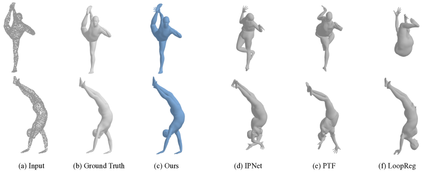
In Table 2 we show quantitative results for the SMPL body estimation task, evaluated in terms of vertex error and joint position error. Note that our results are obtained directly from the network, while the other methods require an optimization step. For OOD data, our model performs significantly better than the rest, reducing the vertex error by almost two times over the best-performing competitor (PTF with augmentation). This shows the importance of including the right symmetries within the network design, which cannot be replaced by simply performing data augmentation. It is worth noting that all the other methods require data augmentation to perform reasonably in the OOD case. While data augmentation slightly improves the results in our case, we outperform the rest even without it. For in-distribution data, ArtEq without data augmentation also surpasses the previous state of the art model by 68% in V2V error, while the competing methods are much slower at inference time due to the optimization step. In the bottom part of Table 2 we show that our proposed parent conditioning consistently improves the results by around 5 mm for OOD samples. Qualitative results can be found in Figure 5.

Additionally, we evaluate our model directly on raw real-world scans from the DFAUST dataset [8], which contains a different noise distribution including sensor noise and holes. For this OOD noise experiment, we perform inference on these scans without fine-tuning our model, and find the part segmentation performance only drops by 5%. While the OOD noise increases the V2V error by 2cm, it is still on par with the accuracy of previous state-of-the-art methods on synthetic data. While ArtEq works well without fine-tuning, we suspect that training on real noise will produce significant improvements in robustness and accuracy. See supplemental material for more information.

Method	#Param (M)	Time (s)
IP-Net [5]	35.0	211.4
LoopReg [6]	3.3	146.9
PTF [54]	34.1	158.1
Ours	0.9	0.1

Table 3: Number of parameters (#Param) and inference time (Time) for the methods evaluated in this paper.

(a) In-distribution

(b) Out-of-distribution

Figure 6: Convergence plots. Vertex-to-vertex error (V2V), joint position error (Joint Error), and part segmentation accuracy (Acc) as a function of epoch number, on (a) in-distribution and (b) out-of-distribution datasets.

5.4 Performance and Convergence

Performance

Table 3 shows computation time for all methods, along with model size. Using SE(3)- equivariant/invariant features allows our model to be more space- and time-efficient. ArtEq has only $2.7\%$ the number of parameters of PTF, while still outperforming in terms of accuracy. Additionally, our smaller model size results in significantly faster inference time, which is three orders of magnitude faster than the others. Of course, like the other methods, one could add an additional optimization step to refine our results further.

Convergence

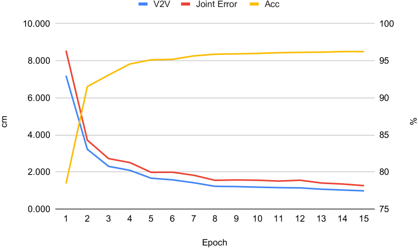
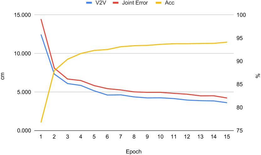
In addition to being computationally faster and having lower memory requirements, we show in Figure 6 that our method also converges rapidly, requiring merely 5 epochs of training to reach reasonable results, for both in-distribution and out-of-distribution datasets.

5.5 Limitations

Our method’s primary failure mode results from self-contact, a disadvantage shared with most mesh registration methods. Here, self-contact may lead to incorrect feature aggregation, where features that belong to different body parts are convolved together due to their proximity in Euclidean space. Additionally, while our method generalizes to unseen rigid transformations of the body parts, the model is not guaranteed to be robust to non-rigid deformations that are encoded in the pose corrective blendshapes of SMPL. Its performance in this respect depends on the distribution of non-rigid transformations seen during training. Though data augmentation is helpful to mitigate the aforementioned limitations, a more principled solution to address these is left for future work.

6 Conclusions

In this paper we propose ArtEq, a powerful part-based SE(3)-equivariant neural framework for SMPL parameter estimation from point clouds. Our experimental results demonstrate the generalization ability of ArtEq to out-of-distribution poses, where the direct regression output of ArtEq outperforms state-of-the-art methods that require a time-consuming test-time optimization step. ArtEq is also significantly more efficient in terms of model parameters and computation. Our results demonstrate the advantage and importance of incorporating the correct symmetries into the task of SMPL-body pose and shape estimation. ArtEq provides the first fast, practical, method to infer SMPL models directly from point clouds. This serves as a foundation to make 3D human mesh registration more accessible and efficient.

Acknowledgements. We thank Yandong Wen, Nikos Athanasiou, Justus Thies, and Timo Bolkart for proofreading and discussion; Xu Chen, Yuxuan Xue, Yao Feng, Weiyang Liu, Zhen Liu, Yuliang Xiu, Shashank Tripathi, Qianli Ma and Hanqi Zhou for their helpful discussions; and the International Max Planck Research School for Intelligent Systems (IMPRS-IS) for supporting PK.

MJB Disclosure

https://files.is.tue.mpg.de/black/CoI_ICCV_2023.txt

Supplementary Material

Appendix A Additional Results

In this section we provide additional results, as well as ablation studies that demonstrate the impact of our design choices.

Qualitative Registration Results

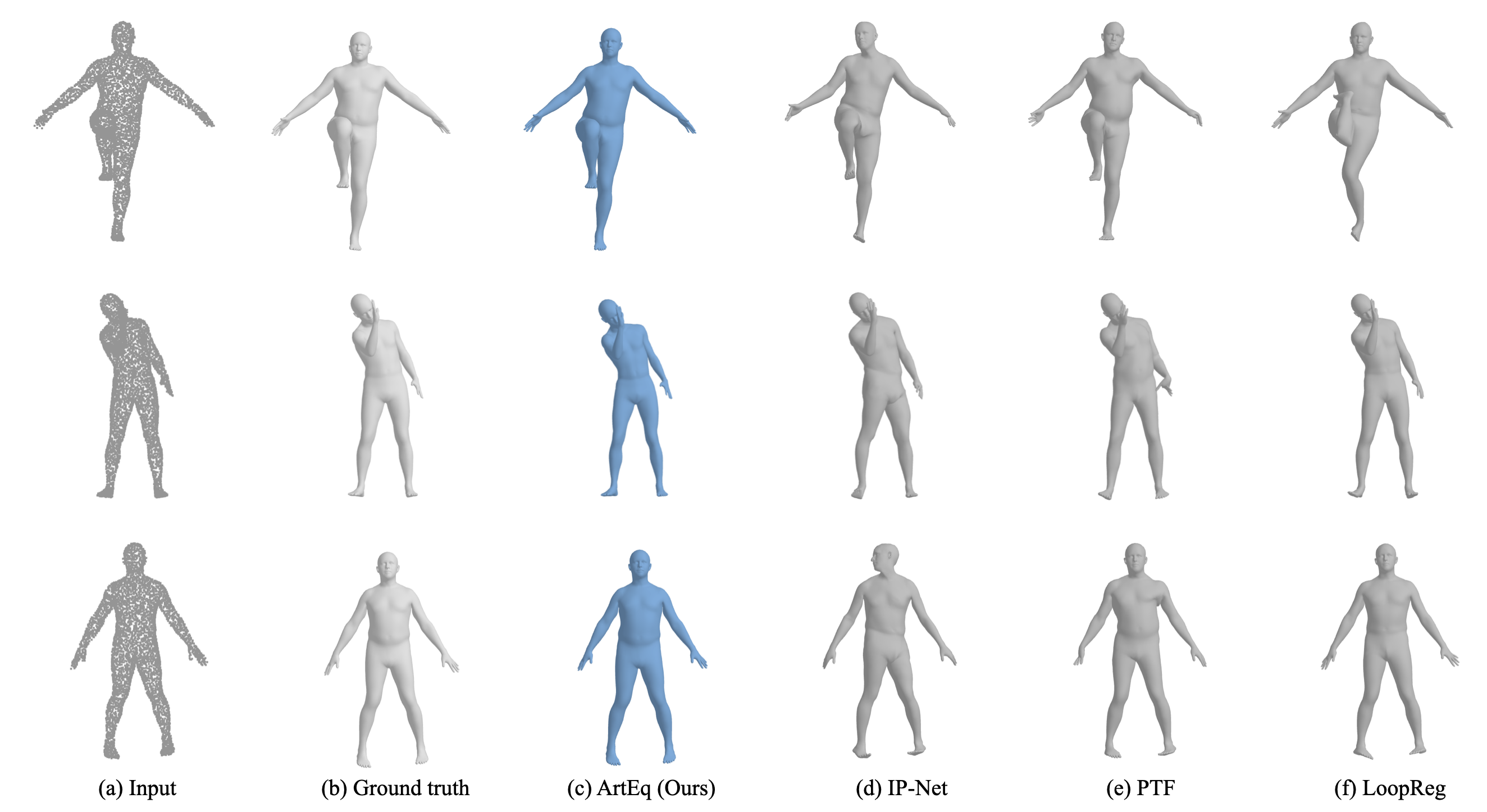
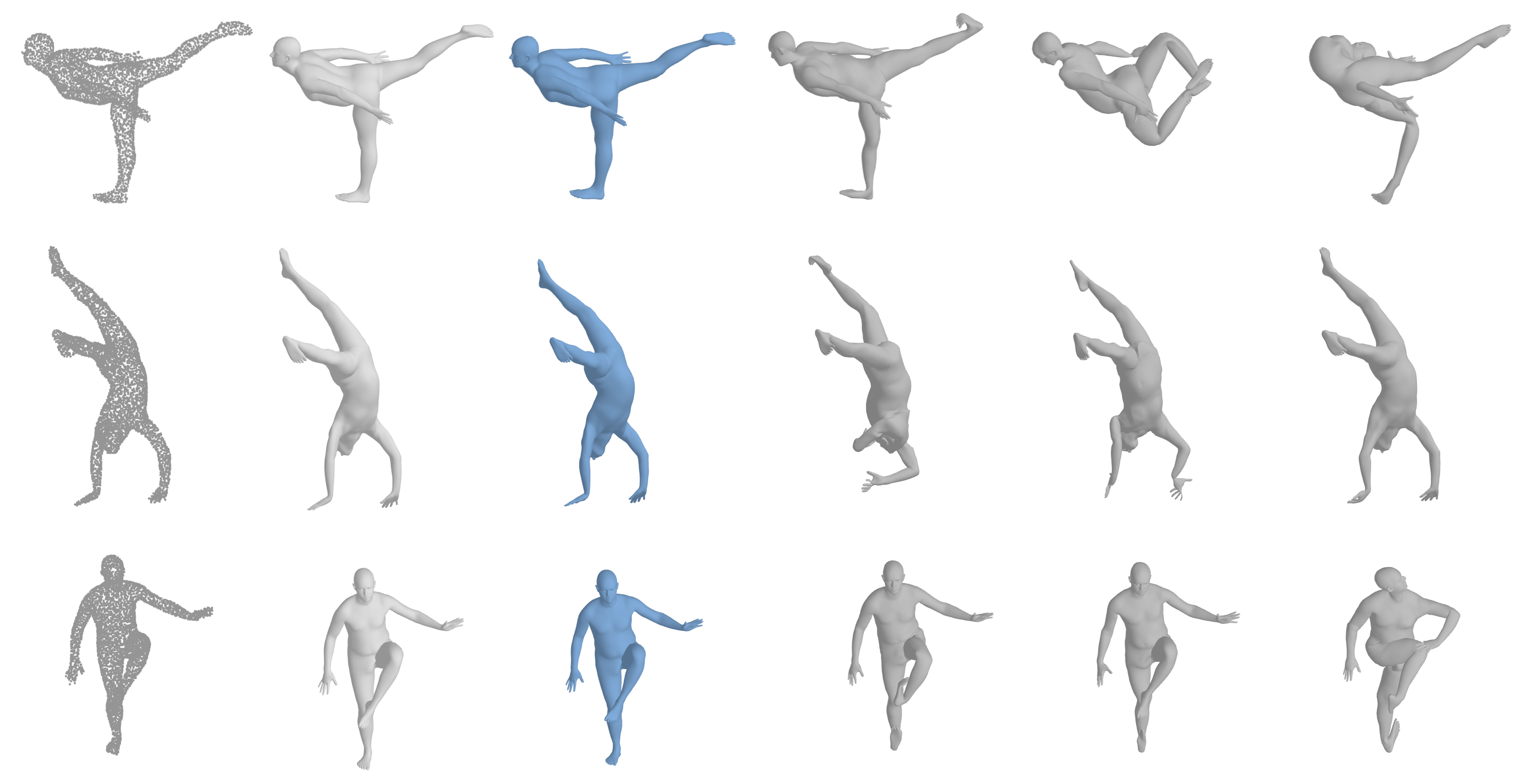
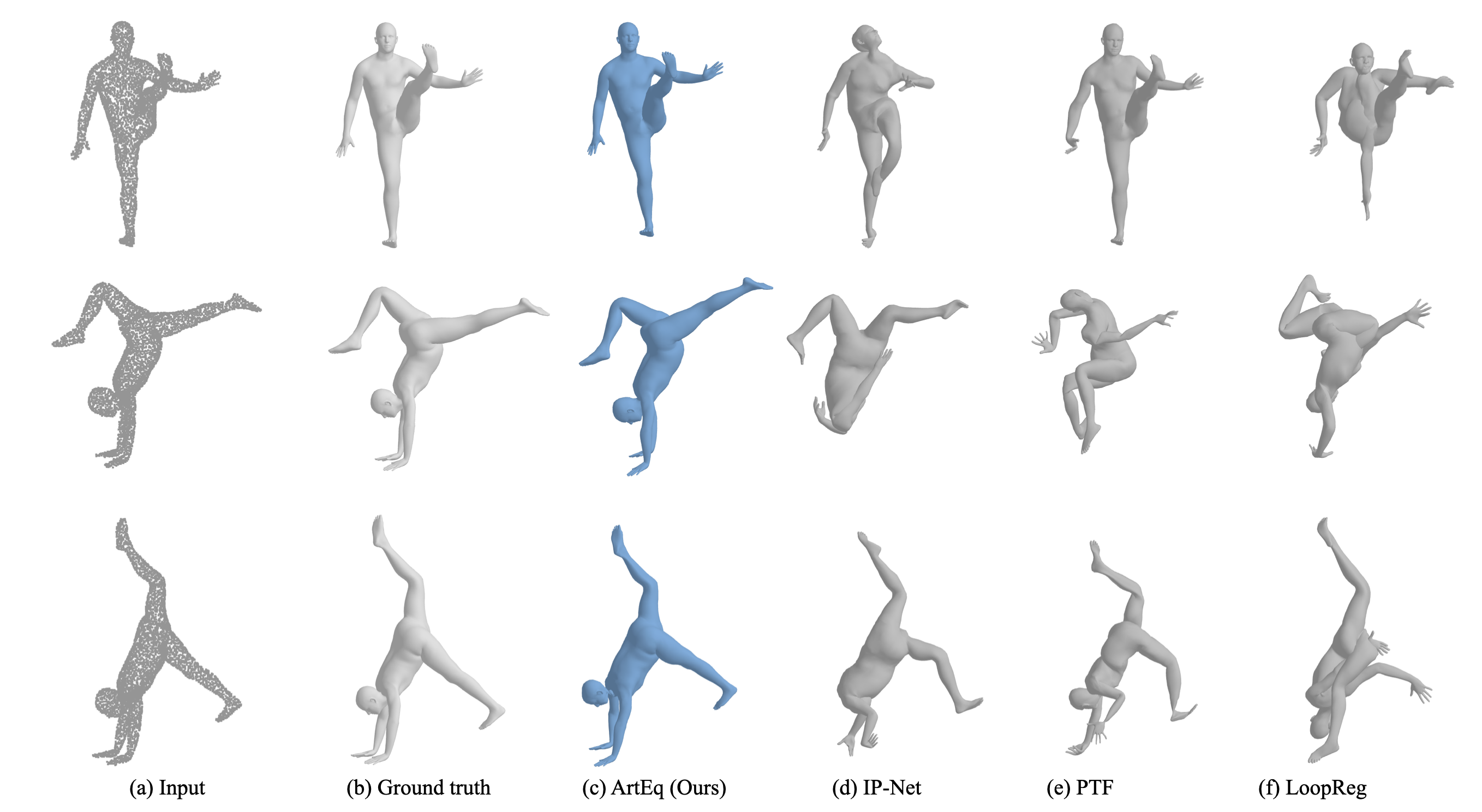
Figure S.2 shows qualitative results for out-of-distribution testing data, and Figure S.1 shows results for the in-distribution case. IP-Net, PTF, and LoopReg all fail under difficult poses, resulting in unnatural rotations for some body parts. Poses that are particularly far from the distribution, such as standing on the arms, result in very unnatural shapes. In contrast, our method can handle such poses well despite never having seen similar ones during training. It is worth noting that LoopReg uses the same self-supervised objective during training and during optimization, and refines the learned correspondences at test time by overfitting to the input. Hence, we see here that even such a test-time optimization strategy is not sufficient when the initial poses are far from the correct result.

Figure S.1: Qualitative results for in-distribution poses. From left to right: (a) input point cloud, (b) ground-truth SMPL mesh, (c) our results, (d) IP-Net [5], (e) PTF [54] and (f) LoopReg [6].

Figure S.2: Qualitative results for out-of-distribution poses. From left to right: (a) input point cloud, (b) ground-truth SMPL mesh, (c) our results, (d) IP-Net [5], (e) PTF [54] and (f) LoopReg [6].

Qualitative Segmentation Results

In Figure S.3

Figure S.3: Qualitative results for part segmentation. From left to right: (a) ground-truth segmentation, (b) our results, (c) IP-Net [5], (d) PTF [54], and (e) LoopReg [6].

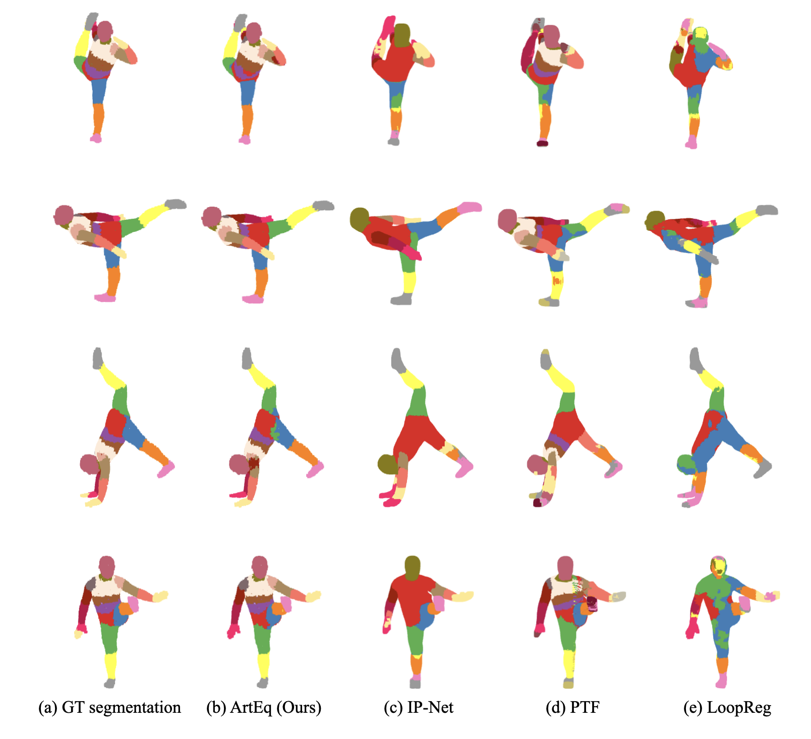
we show additional results for part segmentation on out-of-distribution data, along with comparisons to the segmentations obtained by IP-Net, PTF, and LoopReg. Note that IP-Net and LoopReg predict part segmentation for 14 body parts, where, for example, the two shoulder blades, the three spine regions and the hip are all merged into one torso part (here, in red), or the neck is merged into the head region (here, in olive), making it an easier problem. Our method produces accurate segmentations even for these difficult OOD cases, while PTF, IP-Net, and LoopReg struggle to predict the segmentation, particularly in the regions with out-of-distribution pose. For example, in the second row, IP-Net’s part segmentation confuses left and right, resulting in a flipped torso with the belly facing up.

Raw Scan Data

We evaluated our method on the raw scans from the DFaust testing set (in-distribution), without any fine-tuning or re-training. Our model obtains $88.3\%$ accuracy for part segmentation, $3.62$cm vertex-to-vertex error, and $4.37$cm MPJPE error, which is still better than most other methods on clean data. A qualitative example of these results is shown in Figure S.4. Here we see that our estimations are still accurate for out-of-distribution poses, despite the out-of-distribution noise.

Figure S.4: Qualitative results on the raw scans from DFAUST testing set. From left to right: (a) input point cloud, (b) ground-truth SMPL mesh, (c) our results.

Impact of the Number of Input Points

We show in Table S.1 the results of our model when the input is 500, 1000, 2500, and 5000 points. We see here that our method can already perform reasonably well for in-distribution data for 1000 input points, with a segmentation accuracy that is on par with competitors that use 5000 points as input ($91.2\%$ for IP-Net, Table 1 in main paper). The segmentation accuracy does not differ much when moving to the OOD case. The model has lower performance in terms of V2V and MPJPE for a lower number of points on OOD data, however it still outperforms all the competitors (Table 2 in main paper). This shows that our model does not require a significant number of points in order to obtain accurate results, both for in- and out-of-distribution data.

# points	OOD			ID
	Seg. $\uparrow$	V2V $\downarrow$	MPJPE $\downarrow$	Seg.	V2V $\downarrow$	MPJPE $\downarrow$
500	80.5	7.33	8.63	82.9	4.55	5.27
1000	89.7	4.85	5.83	92.1	2.27	2.80
2500	93.0	4.09	4.59	95.4	1.01	1.22
5000	94.1	3.62	4.23	96.2	0.98	1.26

Table S.1: Our results for different numbers of input points, in terms of segmentation accuracy (“Seg.”), vertex-to-vertex error (“V2V”), and mean joint position error (“MPJPE”).

Baselines Without a Pose Prior

PTF and IP-Net use a pose prior to regularize the pose space when fitting to SMPL. In the main paper we tested these methods with default parameters, which include the use of the pose prior. To make sure that this does not negatively affect the final outcome, we evaluate PTF and IP-Net without the pose prior. The results are shown in Table S.2, where we observe that the pose prior does not have a substantial effect on the output.

Method	Pose Prior	OOD		ID
		V2V $\downarrow$	MPJPE $\downarrow$	V2V $\downarrow$	MPJPE $\downarrow$
IP-Net	$\checkmark$	7.57	9.41	5.98	6.42
IP-Net		7.67	9.55	6.04	6.50
PTF	$\checkmark$	6.42	7.56	3.05	3.53
PTF		6.46	7.62	3.13	3.66
Ours		3.62	4.23	0.98	1.26

Table S.2: Comparison with IP-Net and PTF with and without using their pose prior.

Appendix B Permutation Equivariance of the Self-Attention Mechanism

As we have mentioned in the main paper, a function (network) $f:V\to W$ is said to be equivariant with respect to a group $\mathcal{G}$ if, for any transformation $\mathcal{T}\in\mathcal{G},f(\mathcal{T}\boldsymbol{X})=\mathcal{T}f(\boldsymbol{X})$, $\boldsymbol{X}\in V$. Here we elaborate on how the self-attention function $f_{SA}$ is equivariant to the permutation group $\mathcal{T}(\boldsymbol{X})=\boldsymbol{X}P_{\pi}$, where $P_{\pi}$ denotes the permutation matrix of $\pi$, and $\pi$ denotes the permutation of the input tensor’s elements (in our case, the permutation over the group element dimension). The self-attention function $f_{SA}$ is defined as $f_{SA}(\mathbf{X})=\boldsymbol{W}_{v}\boldsymbol{X}\cdot\operatorname{softmax}\left(\left(\boldsymbol{W}_{k}\boldsymbol{X}\right)^{T}\cdot\boldsymbol{W}_{q}\boldsymbol{X}\right)$, then

$$f_{SA}\left(\mathcal{T}(\boldsymbol{X})\right)$$ (S.1)

$$=\boldsymbol{W}_{v}\mathcal{T}(\boldsymbol{X})\cdot\operatorname{softmax}\left(\left(\boldsymbol{W}_{k}\mathcal{T}(\boldsymbol{X})\right)^{T}\cdot\boldsymbol{W}_{q}\mathcal{T}(\boldsymbol{X})\right)$$

$$=\boldsymbol{W}_{v}\boldsymbol{X}P_{\pi}\cdot\operatorname{softmax}\left(\left(\boldsymbol{W}_{k}\boldsymbol{X}P_{\pi}\right)^{T}\cdot\boldsymbol{W}_{q}\boldsymbol{X}P_{\pi}\right)$$

$$=\boldsymbol{W}_{v}\boldsymbol{X}P_{\pi}\cdot\operatorname{softmax}\left(P_{\pi}^{T}\left(\boldsymbol{W}_{k}\boldsymbol{X}\right)^{T}\cdot\boldsymbol{W}_{q}\boldsymbol{X}P_{\pi}\right)$$

$$=\boldsymbol{W}_{v}\boldsymbol{X}\left(P_{\pi}P_{\pi}^{T}\right)\cdot\operatorname{softmax}\left(\left(\boldsymbol{W}_{k}\boldsymbol{X}\right)^{T}\cdot\boldsymbol{W}_{q}\boldsymbol{X}\right)P_{\pi}$$

$$=\boldsymbol{W}_{v}\boldsymbol{X}\cdot\operatorname{softmax}\left(\left(\boldsymbol{W}_{k}\boldsymbol{X}\right)^{T}\cdot\boldsymbol{W}_{q}\boldsymbol{X}\right)P_{\pi}$$

$$=\mathcal{T}\left(f_{SA}(\boldsymbol{X})\right),$$

where we used the property $\operatorname{softmax}(P\cdot A\cdot P^{T})=P\cdot\operatorname{softmax}(A)\cdot P^{T}$, for a permutation matrix $P$ and an arbitrary matrix $A$, to go from the third to the fourth line (refer to the proof in [58]). Hence, we have proved that the self-attention function is equivariant to the permutation operation over the discretized SO(3) group elements.

Appendix C Method Details

Architecture

The local SO(3) feature extractor has two SPConv layers and a nearest neighbor feature propagation layer [42]. Each SPConv layer has a kernel size of 0.4 and a stride downsampling factor of 2, therefore, the input point cloud with shape [B, N, 3] will be processed as [B, N/4, 64, 60] where the last dimension is the group element obtained by SO(3) discretization, and $C=64$ is the feature dimension. For each input point, the feature propagation layer finds the top 3 spatial nearest neighbors of the downsampled point-wise features, and interpolates these features weighed by their pairwise distance, resulting in an output of size [B, N, 64, 60].

To obtain the chordal mean weights we attach to the self-attention layers an element-wise MLP (3 layers with ReLU, sizes [64,64,1]), since self-attention does not contain non-linear activations. Similarly, we attach a 2-layer MLP on the flattened part features [B, 20*6] to obtain the final SMPL shape code.

Part Segmentation

We consider here 20 body parts, merging the fingers into hands, and toes into feet. This is because the AMASS DFAUST dataset does not contain finger or toe motion.

Averaging Rotations by Calculating the Chordal L2 Mean

Given two rotations $R$ and $S$, the chordal L2 distance is defined as $d_{chord}(R,S)=\lVert R-S\rVert_{F}$ where $\lVert\cdot\rVert_{F}$ is the Frobenius norm of the matrix, which is related to the angular distance between $R$ and $S$ [20]. The chordal L2 mean of a set of rotations is then defined as the matrix that minimizes the chordal distance to all rotations in the set. In our case, if $\mathbf{w}_{k,j}$ is the weight for part $k$ and group $j$, then the weighted average for part $k$ over the $|\mathcal{G}|=60$ rotation symmetries is

$$\operatorname*{arg\,min}_{\hat{\mathcal{R}}_{k}\in SO(3)}\sum_{j=1}^{\lvert\mathcal{G}\rvert}d_{chord}(\mathbf{w}_{k,j}\cdot\mathcal{R}(\mathbf{g}_{j}),\hat{\mathcal{R}}_{k})$$ (S.2)

where $\mathcal{R}(\mathbf{g}_{j})$ is the rotation matrix of $\mathbf{g}_{j}$, and $\mathbf{g}_{j}$ is a group element. In practice, $\hat{\mathcal{R}}_{k}$ can be obtained in closed-form by using singular value decomposition. We refer the readers to [20] for more details.

Loss Function

We train both stages of the network with the following loss function:

$$\lambda_{1}\mathcal{L}_{pose}+\lambda_{2}\mathcal{L}_{shape}+\lambda_{3}\mathcal{L}_{verts}+\lambda_{4}\mathcal{L}_{joint}+\lambda_{5}\mathcal{L}_{part},$$ (S.3)

where

• $\mathcal{L}_{pose}=||\tilde{\boldsymbol{\theta}}-\boldsymbol{\theta}||^{2}$ is the MSE loss between predicted pose coefficients $\tilde{\boldsymbol{\theta}}$ and ground-truth pose coefficients $\boldsymbol{\theta}$.

• $\mathcal{L}_{shape}=||\tilde{\boldsymbol{\beta}}-\boldsymbol{\beta}||^{2}$ is the MSE loss between predicted shape coefficients $\tilde{\boldsymbol{\beta}}$ and ground-truth shape coefficients $\boldsymbol{\beta}$.

• $\mathcal{L}_{verts}=||\mathcal{W}\left(M(\tilde{\boldsymbol{\beta}},\tilde{\boldsymbol{\theta}})-M(\boldsymbol{\beta},\boldsymbol{\theta})\right)||^{2}$ is the weighted MSE loss between the reconstructed SMPL mesh vertices and the ground-truth registration, using the per-vertex weights $\mathcal{W}$, where the vertices corresponding to body markers are assigned a weight of 2.0, and the other vertices a weight of 1.0.

• $\mathcal{L}_{joint}=||\mathcal{T}(\mathcal{J}(\tilde{\boldsymbol{\beta}}),\tilde{\boldsymbol{\theta}})-\mathcal{T}(\mathcal{J}(\boldsymbol{\beta}),\boldsymbol{\theta})||^{2}$ is the MSE loss between the predicted joint positions of the SMPL mesh (posed) and the ground-truth joint positions.

• $\mathcal{L}_{part}=\operatorname{cross-entropy}(\alpha(\mathbf{x}_{i},\mathbf{p}_{k}),\alpha_{gt}(\mathbf{x}_{i},\mathbf{p}_{k}))$ is the cross-entropy loss between the predicted part segmentation and the ground-truth part segmentation of the point cloud.

We use $\lambda_{1}=5$, $\lambda_{2}=50$, $\lambda_{3}=100$, $\lambda_{4}=100$, $\lambda_{5}=5$.

References

- [1] Ijaz Akhter and Michael J. Black. Pose-conditioned joint angle limits for 3D human pose reconstruction. In Computer Vision and Pattern Recognition (CVPR), pages 1446–1455, 2015.
- [2] Brett Allen, Brian Curless, and Zoran Popović. The space of human body shapes: Reconstruction and parameterization from range scans. ACM Transactions on Graphics, 22(3):587–594, 2003.
- [3] Dragomir Anguelov, Praveen Srinivasan, Daphne Koller, Sebastian Thrun, Jim Rodgers, and James Davis. SCAPE: Shape completion and animation of people. In ACM Transactions on Graphics (Proceedings of SIGGRAPH), pages 408–416. ACM New York, NY, USA, 2005.
- [4] Matan Atzmon, Koki Nagano, Sanja Fidler, Sameh Khamis, and Yaron Lipman. Frame averaging for equivariant shape space learning. In Computer Vision and Pattern Recognition (CVPR), pages 631–641, 2022.
- [5] Bharat Lal Bhatnagar, Cristian Sminchisescu, Christian Theobalt, and Gerard Pons-Moll. Combining implicit function learning and parametric models for 3D human reconstruction. In European Conference on Computer Vision (ECCV). Springer, August 2020.
- [6] Bharat Lal Bhatnagar, Cristian Sminchisescu, Christian Theobalt, and Gerard Pons-Moll. LoopReg: Self-supervised learning of implicit surface correspondences, pose and shape for 3D human mesh registration. Conference on Neural Information Processing Systems (NeurIPS), 33:12909–12922, 2020.
- [7] Federica Bogo, Javier Romero, Matthew Loper, and Michael J. Black. FAUST: Dataset and evaluation for 3D mesh registration. In Computer Vision and Pattern Recognition (CVPR), pages 3794–3801, 2014.
- [8] Federica Bogo, Javier Romero, Gerard Pons-Moll, and Michael J. Black. Dynamic FAUST: Registering human bodies in motion. In Computer Vision and Pattern Recognition (CVPR), July 2017.
- [9] Haiwei Chen, Shichen Liu, Weikai Chen, Hao Li, and Randall Hill. Equivariant point network for 3D point cloud analysis. In Computer Vision and Pattern Recognition (CVPR), pages 14514–14523, 2021.
- [10] Xu Chen, Yufeng Zheng, Michael J. Black, Otmar Hilliges, and Andreas Geiger. SNARF: Differentiable forward skinning for animating non-rigid neural implicit shapes. In International Conference on Computer Vision (ICCV), pages 11594–11604, 2021.
- [11] Yang Chen and Gérard Medioni. Object modelling by registration of multiple range images. Image and Vision Computing, 10(3):145–155, 1992.
- [12] Taco Cohen, Maurice Weiler, Berkay Kicanaoglu, and Max Welling. Gauge equivariant convolutional networks and the icosahedral CNN. In International Conference on Machine Learning (ICML), pages 1321–1330. PMLR, 2019.
- [13] Taco Cohen and Max Welling. Group equivariant convolutional networks. In International Conference on Machine Learning (ICML), pages 2990–2999. PMLR, 2016.
- [14] Taco S. Cohen, Mario Geiger, Jonas Köhler, and Max Welling. Spherical CNNs. In International Conference on Learning Representations (ICLR), 2018.
- [15] Bailin Deng, Yuxin Yao, Roberto M. Dyke, and Juyong Zhang. A survey of non-rigid 3D registration. Computer Graphics Forum, 2022.
- [16] Congyue Deng, Or Litany, Yueqi Duan, Adrien Poulenard, Andrea Tagliasacchi, and Leonidas J. Guibas. Vector neurons: A general framework for SO(3)-equivariant networks. In International Conference on Computer Vision (ICCV), pages 12200–12209, 2021.
- [17] Carlos Esteves, Christine Allen-Blanchette, Ameesh Makadia, and Kostas Daniilidis. Learning SO(3) equivariant representations with spherical CNNs. In European Conference on Computer Vision (ECCV), pages 52–68, 2018.
- [18] Fabian Fuchs, Daniel Worrall, Volker Fischer, and Max Welling. SE(3)-transformers: 3D roto-translation equivariant attention networks. Conference on Neural Information Processing Systems (NeurIPS), 33:1970–1981, 2020.
- [19] Thibault Groueix, Matthew Fisher, Vladimir G. Kim, Bryan C. Russell, and Mathieu Aubry. 3D-CODED: 3D correspondences by deep deformation. In European Conference on Computer Vision (ECCV), pages 230–246, 2018.
- [20] Richard Hartley, Jochen Trumpf, Yuchao Dai, and Hongdong Li. Rotation averaging. International Journal of Computer Vision (IJCV), 103:267–305, 2013.
- [21] David A. Hirshberg, Matthew Loper, Eric Rachlin, and Michael J. Black. Coregistration: Simultaneous alignment and modeling of articulated 3D shape. In European Conference on Computer Vision (ECCV), LNCS 7577, Part IV, pages 242–255. Springer-Verlag, Oct. 2012.
- [22] Tomas Hodan, Daniel Barath, and Jiri Matas. EPOS: Estimating 6D pose of objects with symmetries. In Computer Vision and Pattern Recognition (CVPR), June 2020.
- [23] Boyan Jiang, Yinda Zhang, Xingkui Wei, Xiangyang Xue, and Yanwei Fu. H4D: Human 4D modeling by learning neural compositional representation. In Computer Vision and Pattern Recognition (CVPR), pages 19355–19365, 2022.
- [24] Haiyong Jiang, Jianfei Cai, and Jianmin Zheng. Skeleton-aware 3D human shape reconstruction from point clouds. In International Conference on Computer Vision (ICCV), pages 5431–5441, 2019.
- [25] Hanbyul Joo, Tomas Simon, and Yaser Sheikh. Total Capture: A 3D deformation model for tracking faces, hands, and bodies. In Computer Vision and Pattern Recognition (CVPR), pages 8320–8329, 2018.
- [26] Oren Katzir, Dani Lischinski, and Daniel Cohen-Or. Shape–pose disentanglement using SE(3)-equivariant vector neurons. In European Conference on Computer Vision (ECCV), 2022.
- [27] Nicolas Keriven and Gabriel Peyré. Universal invariant and equivariant graph neural networks. Conference on Neural Information Processing Systems (NeurIPS), 32, 2019.
- [28] Chun-Liang Li, Tomas Simon, Jason Saragih, Barnabás Póczos, and Yaser Sheikh. LBS autoencoder: Self-supervised fitting of articulated meshes to point clouds. In Computer Vision and Pattern Recognition (CVPR), pages 11967–11976, 2019.
- [29] Xiaolong Li, Yijia Weng, Li Yi, Leonidas J. Guibas, A. Abbott, Shuran Song, and He Wang. Leveraging SE(3) equivariance for self-supervised category-level object pose estimation from point clouds. Conference on Neural Information Processing Systems (NeurIPS), 34:15370–15381, 2021.
- [30] Guanze Liu, Yu Rong, and Lu Sheng. VoteHMR: Occlusion-aware voting network for robust 3D human mesh recovery from partial point clouds. In Proceedings of the 29th ACM International Conference on Multimedia, pages 955–964, 2021.
- [31] Matthew Loper, Naureen Mahmood, Javier Romero, Gerard Pons-Moll, and Michael J. Black. SMPL: A skinned multi-person linear model. ACM Transactions on Graphics (Proceedings of SIGGRAPH Asia), 34(6):248:1–248:16, Oct. 2015.
- [32] Matthew M. Loper, Naureen Mahmood, and Michael J. Black. MoSh: Motion and shape capture from sparse markers. ACM Transactions on Graphics (Proceedings of SIGGRAPH Asia), 33(6):220:1–220:13, Nov. 2014.
- [33] Shitong Luo, Jiahan Li, Jiaqi Guan, Yufeng Su, Chaoran Cheng, Jian Peng, and Jianzhu Ma. Equivariant point cloud analysis via learning orientations for message passing. In Computer Vision and Pattern Recognition (CVPR), pages 18932–18941, 2022.
- [34] Naureen Mahmood, Nima Ghorbani, Nikolaus F. Troje, Gerard Pons-Moll, and Michael J. Black. AMASS: Archive of motion capture as surface shapes. In International Conference on Computer Vision (ICCV), pages 5442–5451, Oct. 2019.
- [35] Priyanka Patel, Chun-Hao P. Huang, Joachim Tesch, David T. Hoffmann, Shashank Tripathi, and Michael J. Black. AGORA: Avatars in geography optimized for regression analysis. In Computer Vision and Pattern Recognition (CVPR), pages 13463–13473, Piscataway, NJ, June 2021. IEEE.
- [36] Sida Peng, Junting Dong, Qianqian Wang, Shangzhan Zhang, Qing Shuai, Xiaowei Zhou, and Hujun Bao. Animatable neural radiance fields for modeling dynamic human bodies. In International Conference on Computer Vision (ICCV), pages 14314–14323, 2021.
- [37] Leonid Pishchulin, Stefanie Wuhrer, Thomas Helten, Christian Theobalt, and Bernt Schiele. Building statistical shape spaces for 3D human modeling. Pattern Recognition, 67:276–286, 2017.
- [38] Gerard Pons-Moll, Javier Romero, Naureen Mahmood, and Michael J. Black. Dyna: A model of dynamic human shape in motion. ACM Transactions on Graphics (Proceedings of SIGGRAPH Asia), 34(4):120:1–120:14, Aug. 2015.
- [39] Sergey Prokudin, Christoph Lassner, and Javier Romero. Efficient learning on point clouds with basis point sets. In Computer Vision and Pattern Recognition (CVPR), pages 4332–4341, 2019.
- [40] Omri Puny, Matan Atzmon, Edward J. Smith, Ishan Misra, Aditya Grover, Heli Ben-Hamu, and Yaron Lipman. Frame averaging for invariant and equivariant network design. In International Conference on Learning Representations (ICLR), 2021.
- [41] Charles R. Qi, Hao Su, Kaichun Mo, and Leonidas J. Guibas. PointNet: Deep learning on point sets for 3D classification and segmentation. In Computer Vision and Pattern Recognition (CVPR), pages 652–660, 2017.
- [42] Charles R. Qi, Li Yi, Hao Su, and Leonidas J. Guibas. PointNet++: Deep hierarchical feature learning on point sets in a metric space. Conference on Neural Information Processing Systems (NeurIPS), 30, 2017.
- [43] Akiyoshi Sannai, Makoto Kawano, and Wataru Kumagai. Equivariant and invariant Reynolds networks. ArXiv, abs/2110.08092, 2021.
- [44] Vıctor G. Satorras, Emiel Hoogeboom, and Max Welling. E(n) equivariant graph neural networks. In International Conference on Machine Learning (ICML), pages 9323–9332. PMLR, 2021.
- [45] Anthony Simeonov, Yilun Du, Andrea Tagliasacchi, Joshua B. Tenenbaum, Alberto Rodriguez, Pulkit Agrawal, and Vincent Sitzmann. Neural descriptor fields: SE(3)-equivariant object representations for manipulation. In International Conference on Robotics and Automation (ICRA), pages 6394–6400. IEEE, 2022.
- [46] Ivan Sosnovik, Michał Szmaja, and Arnold Smeulders. Scale-equivariant steerable networks. In International Conference on Learning Representations (ICLR), 2020.
- [47] Riccardo Spezialetti, Federico Stella, Marlon Marcon, Luciano Silva, Samuele Salti, and Luigi Di Stefano. Learning to orient surfaces by self-supervised spherical CNNs. Conference on Neural Information Processing Systems (NeurIPS), 33:5381–5392, 2020.
- [48] Hugues Thomas, Charles R. Qi, Jean-Emmanuel Deschaud, Beatriz Marcotegui, Francois Goulette, and Leonidas J. Guibas. KPConv: Flexible and deformable convolution for point clouds. In International Conference on Computer Vision (ICCV), October 2019.
- [49] Nathaniel Thomas, Tess Smidt, Steven Kearnes, Lusann Yang, Li Li, Kai Kohlhoff, and Patrick Riley. Tensor field networks: Rotation- and translation-equivariant neural networks for 3D point clouds. arXiv preprint arXiv:1802.08219, 2018.
- [50] Garvita Tiwari, Nikolaos Sarafianos, Tony Tung, and Gerard Pons-Moll. Neural-GIF: Neural generalized implicit functions for animating people in clothing. In International Conference on Computer Vision (ICCV), pages 11708–11718, 2021.
- [51] Aggeliki Tsoli, Matthew Loper, and Michael J. Black. Model-based anthropometry: Predicting measurements from 3D human scans in multiple poses. In Winter Conference on Applications of Computer Vision (WACV), pages 83–90. IEEE, Mar. 2014.
- [52] Haiping Wang, Yuan Liu, Zhen Dong, and Wenping Wang. You only hypothesize once: Point cloud registration with rotation-equivariant descriptors. In Proceedings of the 30th ACM International Conference on Multimedia, pages 1630–1641, 2022.
- [53] Kangkan Wang, Jin Xie, Guofeng Zhang, Lei Liu, and Jian Yang. Sequential 3D human pose and shape estimation from point clouds. In Computer Vision and Pattern Recognition (CVPR), pages 7275–7284, 2020.
- [54] Shaofei Wang, Andreas Geiger, and Siyu Tang. Locally aware piecewise transformation fields for 3D human mesh registration. In Computer Vision and Pattern Recognition (CVPR), pages 7639–7648, 2021.
- [55] Shaofei Wang, Katja Schwarz, Andreas Geiger, and Siyu Tang. ARAH: Animatable volume rendering of articulated human SDFs. In European Conference on Computer Vision (ECCV), pages 1–19, Cham, 2022. Springer Nature Switzerland.
- [56] Maurice Weiler, Fred A. Hamprecht, and Martin Storath. Learning steerable filters for rotation equivariant CNNs. In Computer Vision and Pattern Recognition (CVPR), pages 849–858, 2018.
- [57] Michael C. Wong, Jonathan P. Bennett, Lambert T. Leong, Isaac Y. Tian, Yong E. Liu, Nisa N. Kelly, Cassidy McCarthy, Julia M.W. Wong, Cara B. Ebbeling, David S. Ludwig, Brian A. Irving, Matthew C. Scott, James Stampley, Brett Davis, Neil Johannsen, Rachel Matthews, Cullen Vincellette, Andrea K. Garber, Gertraud Maskarinec, Ethan Weiss, Jennifer Rood, Alyssa N. Varanoske, Stefan M. Pasiakos, Steven B. Heymsfield, and John A. Shepherd. Monitoring body composition change for intervention studies with advancing 3D optical imaging technology in comparison to dual-energy X-ray absorptiometry. The American Journal of Clinical Nutrition, 2023.
- [58] Jiancheng Yang, Qiang Zhang, Bingbing Ni, Linguo Li, Jinxian Liu, Mengdie Zhou, and Qi Tian. Modeling point clouds with self-attention and Gumbel subset sampling. In Computer Vision and Pattern Recognition (CVPR), pages 3323–3332, 2019.
- [59] Manzil Zaheer, Satwik Kottur, Siamak Ravanbakhsh, Barnabas Poczos, Russ R. Salakhutdinov, and Alexander J. Smola. Deep sets. Conference on Neural Information Processing Systems (NeurIPS), 30, 2017.
- [60] Boyao Zhou, Jean-Sébastien Franco, Federica Bogo, Bugra Tekin, and Edmond Boyer. Reconstructing human body mesh from point clouds by adversarial GP network. In Asian Conference on Computer Vision (ACCV), 2020.
- [61] Minghan Zhu, Maani Ghaffari, and Huei Peng. Correspondence-free point cloud registration with SO(3)-equivariant implicit shape representations. In Conference on Robot Learning, pages 1412–1422. PMLR, 2022.
- [62] Silvia Zuffi and Michael J. Black. The stitched puppet: A graphical model of 3D human shape and pose. In Computer Vision and Pattern Recognition (CVPR), pages 3537–3546, 2015.