Contrastive Tuning: A Little Help to Make Masked Autoencoders Forget

Abstract

Masked Image Modeling (MIM) methods, like Masked Autoencoders (MAE), efficiently learn a rich representation of the input. However, for adapting to downstream tasks, they require a sufficient amount of labeled data since their rich features code not only objects but also less relevant image background. In contrast, Instance Discrimination (ID) methods focus on objects. In this work, we study how to combine the efficiency and scalability of MIM with the ability of ID to perform downstream classification in the absence of large amounts of labeled data. To this end, we introduce Masked Autoencoder Contrastive Tuning (MAE–CT), a sequential approach that utilizes the implicit clustering of the Nearest Neighbor Contrastive Learning (NNCLR) objective to induce abstraction in the topmost layers of a pre-trained MAE. MAE–CT tunes the rich features such that they form semantic clusters of objects without using any labels. Notably, MAE–CT does not rely on hand-crafted augmentations and frequently achieves its best performances while using only minimal augmentations (crop & flip). Further, MAE–CT is compute efficient as it requires at most 10% overhead compared to MAE pre-training. Applied to large and huge Vision Transformer (ViT) models, MAE–CT excels over previous self-supervised methods trained on ImageNet in linear probing, $k$-NN and low-shot classification accuracy as well as in unsupervised clustering accuracy. With ViT-H/16 MAE–CT achieves a new state-of-the-art in linear probing of 82.2%.

\begin{overpic}[width=238.48886pt]{figures/teaser_overpic.pdf} \scriptsize \put(3.0,-5.0){food} \put(53.0,-5.0){animals} \put(107.0,-5.0){vehicles} \put(159.0,-5.0){household} \put(222.0,-5.0){nature} \put(33.0,133.0){MAE: 11.1\%} \put(162.0,133.0){MAE-CT: 58.0\%} \end{overpic}

Figure 1: Formation of clusters induced by Masked Autoencoder Contrastive Tuning (MAE–CT). MAE leads to a coarse clustering of objects, in the form of ImageNet super-classes, like food, animals, vehicles, household objects, or objects in nature, that summarize several classes. MAE–CT forms object-specific clusters and thereby improves the $k$-means cluster accuracy w.r.t. the 1000 ImageNet ground truth classes from 11.1% to 58.0% without labeled data or image augmentations based on expert knowledge.

1 Introduction

Self-supervised learning (SSL) leverages a pre-training task on unlabeled data to construct rich representations of the input without explicit supervision from costly annotated labels. This pre-trained representation can then be used to solve downstream tasks, like image classification, better than supervised training only. Therefore, SSL is currently one of the most effective machine learning concepts.

Two of the most prominent SSL pre-training tasks in computer vision are Instance Discrimination (ID) and Masked Image Modeling (MIM). ID uses augmentations to create multiple views of an image. The objective is then to align the views created from the same image. To avoid the trivial solution of mapping all images to a constant representation, methods either use a contrastive loss term [38, 16], a regularization term [92] or perform self-distillation [35, 12]. When a contrastive loss term is used, the ID task can be viewed as a classification task where each image is its own class. MIM methods, like Masked Autoencoders (MAE) [37] and others [7, 87, 6] first mask out areas of the input and then reconstruct the missing parts as pre-train task.

The respective pre-training tasks, classification and reconstruction, of ID and MIM result in distinct advantages and disadvantages. MAE provides a computationally efficient way to exploit sparse pre-training of Vision Transformers (ViT) [28] by masking large parts of the image (75%) and not processing the masked areas. This computational efficiency, coupled with the data efficiency of a generative reconstruction task [88, 30], enabled beneficial scaling to larger architectures on datasets of limited size. However, to perform well on downstream tasks, MIM methods rely on fine-tuning with a large amount of labeled data as the representation of MIM methods lack abstraction after pre-training. In contrast, ID methods learn an object-focused representation [12] that typically results in object-specific clusters which is especially useful when few labels are available, as decision boundaries can be drawn much easier between well separated clusters. Furthermore, ID methods notoriously rely on augmentations based on expert knowledge [76] to alleviate the problem of shortcut learning [33], which refers to the phenomenon of overfitting to spurious features. For example, models could easily learn to extract the color histogram of images to solve the ID task well. To learn more semantic features than a color histogram, color augmentations are essential for almost all ID methods. MIM suffers less from this issue as all masked parts have to be reconstructed, leaving little room for shortcut solutions. In fact, MAE achieves its best performance when only minimal augmentations (crop & flip) are used.

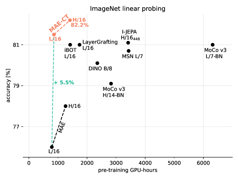
Figure 2: ImageNet linear probing of the best reported models from other self-supervised methods. MAE–CT is able to form a well-clustered representation using little compute.

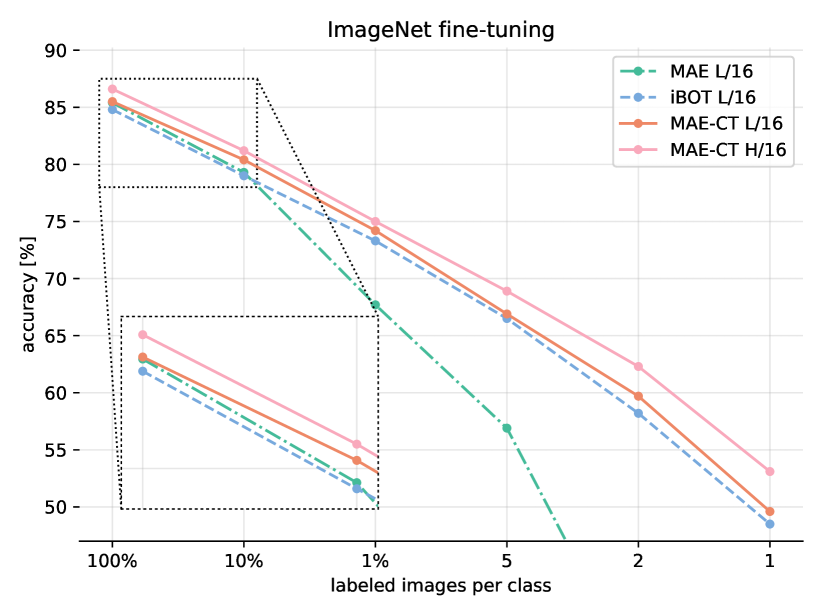
Figure 3: Fine-tuning evaluation on ImageNet. We compare against the best publicly available ID model (iBOT L/16). MAE achieves good performances when given enough labels but struggles otherwise. MAE–CT is able to surpass both MAE and iBOT on all benchmarks. The improvement increases when considering a similar computational budget (MAE–CT H/16) instead of equal model size.

Given the benefits and downsides of both approaches, an open question remains: What is the best combination of MIM and ID methods to exploit their respective strengths? Namely, use the unlabeled data and compute efficiency of MIM methods to benefit from larger models while also benefiting from the label efficiency of ID methods for good low-shot performance via a meaningful semantic representation. Also, extensive augmentations should be optional as they restrict the field of applications and make the models invariant to potentially useful information. The straightforward combination of MIM and ID in an end-to-end fashion faces the issue that the objectives and hyperparameters are heavily conflicting. For example, MIM benefits from high masking ratios and minimal augmentations while ID benefits from less masking and extensive augmentations.

We propose a sequential self-supervised approach to combine MIM and ID methods named Masked Autoencoder Contrastive Tuning (MAE–CT). Contrastive tuning (CT) aims to imitate fine-tuning in the absence of labeled training samples. MAE–CT utilizes a contrastive objective to guide a pre-trained MAE encoder to form semantic clusters, visualized in Figure 1. Unlike previous works, MAE–CT uses the contrastive objective not to learn basic features, but to induce abstraction in the top-half layers of the pre-trained ViT model. This novel setting benefits from multiple adaptations.

State-of-the-art ID methods heavily rely on compute-heavy techniques like multi-crop augmentation [11], a momentum encoder [38] and long training schedules. We do not rely on these compute-heavy techniques and CT takes only a small fraction of the pre-training duration, consequently, MAE–CT adds only little overhead to MAE pre-training as depicted in Figure 2.

Nevertheless, we find that the disentanglement of feature learning (via MAE pre-training) and abstraction (via contrastive tuning) produces well separated clusters. Thus, MAE–CT enables a more label efficient downstream classification than the best ID methods, see Figure 3.

Finally, we adapt the contrastive method Nearest Neighbor Contrastive Learning (NNCLR) [29]. NNCLR extends SimCLR[16] with a queue that holds feature vectors of past samples and a Nearest Neighbor (NN) lookup operation. We observe that this feature space augmentation of NNCLR in combination with our sequential approach and scaling of the model size renders the use of extensive input augmentations based on expert knowledge optional rather than mandatory.

We provide the following contributions:

1. We introduce MAE–CT, a novel computationally efficient and scaleable approach, to form object-related clusters in the representations of pre-trained MAE encoders.

2. We demonstrate that our compute efficient sequential approach is able to surpass the label efficiency of state-of-the-art ID methods in downstream classification.

3. We find that combined pre-training with minimal augmentations suffers from short-cut learning, providing further evidence for the need of our sequential approach.

\begin{overpic}[width=472.01192pt]{figures/overview_mae_ct_v3.pdf} \scriptsize \put(10.0,167.0){{masked image modeling}} \put(16.0,193.8){{encoder}} \put(69.0,193.8){{MIM}} \put(10.0,102.0){{instance discrimination}} \put(16.0,128.8){{encoder}} \put(72.0,128.8){{ID}} \put(30.0,19.0){{combined}} \put(16.0,55.5){{encoder}} \put(69.0,70.2){{MIM}} \put(72.0,41.3){{ID}} \put(123.0,195.0){{encoder}} \put(176.0,195.0){{MIM}} \put(123.0,154.0){{encoder}} \put(179.0,154.0){{ID}} \put(123.0,112.0){{encoder}} \put(179.0,112.0){{ID}} \put(127.0,88.0){{{contrastive tuning}}} \put(132.0,57.0){{frozen layers}} \put(132.0,40.0){{LR decay}} \put(132.0,23.0){{copy weights}} \put(28.0,4.0){{{end-to-end}}} \put(124.0,4.0){{{sequential (MAE-CT)}}} \par\put(330.0,4.0){{{contrastive tuning}}} \put(256.0,96.4){{projector}} \put(256.0,122.0){{projector}} \put(359.0,96.4){{predictor}} \put(432.0,104.0){$z_{i}^{+}$} \put(301.0,128.0){$z_{i}$} \put(385.0,128.0){$\text{topk-NN}(z_{i},Q,k)$} \put(461.0,109.0){$\mathcal{L}_{i}^{\text{NNCLR}}$} \put(372.0,156.0){{queue} $Q$} \put(338.0,216.0){{query}} \put(338.0,205.0){{shift in/out}} \put(388.0,216.0){{sample in $Q$}} \put(388.0,205.0){{selecting sample from topk}} \put(475.0,31.0){$x_{i}$} \put(475.0,62.0){$x_{i}^{+}$} \put(276.0,33.0){{frozen layers}} \put(272.0,53.0){{trainable layers}} \end{overpic}

Figure 4: Contrary to end-to-end methods, MAE–CT is a sequential approach, as depicted on the left side. First, an encoder is pre-trained with a MIM objective (MAE). Afterwards, a NNCLR head is initialized on top of said pre-trained encoder by freezing the encoder and training the NNCLR head until its latent representation is well structured. Finally, contrastive tuning is applied for a short duration. In contrastive tuning, depicted on the right side, we freeze the bottom half of the ViT-encoder and apply a layer-wise learning rate decay for the top half. Two views of one image are generated and then encoded by the ViT. Both encodings are fed into a projector, followed by either a predictor or a topk-NN lookup resulting in the embeddings for the NNCLR loss. The queue $Q$ is updated with the new embeddings in a first in – first out manner after each gradient update step.

2 Related Work

Critical to our sequential approach are the two components MAE [37] and NNCLR [29] on which we build upon. We refer the reader to the respective publications and provide some additional background information in Appendix C. Hereafter, We discuss the most relevant works that make use of both MIM and ID ideas.

The benefit of extending ID with MIM concepts is well established. iBOT [95] adds an auxiliary per-patch reconstruction task. MSN [3] uses masking to improve computational efficiency and augmentation strength. Consequently, these methods report state-of-the-art results in feature and low-shot evaluation. We show that the data efficiency and scaling of MAE enables MAE–CT to exceed these results.

The advances in MIM motivated multiple works that extend MIM methods with ID concepts. CMAE [46] and BootMAE [27] study the addition of an auxiliary ID objective to MAE pre-training. Both approaches improve the fine-tuning performance of ViT-B models, but at the cost of decreased computational efficiency and increased reliance on expert augmentations. They do not report results on larger models, the focus of this work, which would be of interest to measure scalability and data efficiency.

Most related to our approach is the recent work Layer Grafting [50] which also combines MIM and ID into a sequential approach. MAE pre-training is followed by the full training routine of MoCo v3 [18] with an additional regularization loss to keep the lower layer weights close to the MAE weights. In contrast to Layer Grafting, MAE–CT prepares the ID component before changes to the encoder are made, which is then followed up by a short tuning phase. Thus, MAE–CT is much more compute efficient (see Figure 2). For example, the ID part of Layer Grafting requires 15 times the compute of contrastive tuning with a ViT-L/16.

The goal to pre-train larger ViT models with limited use of hand-crafted augmentations is pursued as well in the recent work I-JEPA [4]. I-JEPA models the self-supervised task as a local reconstruction task in feature space.

3 Method

”An autoencoder wants to remember everything a classifier wants to forget.” [31]

Motivation.

MIM approaches are able to train large ViT models, that lack the inductive bias of convolutional neural networks, and learn rich representations just from ImageNet  [37, 6, 87, 73]. However, MIM models rely on adaptation to the downstream tasks using supervised training where performances heavily degrades as the number of labeled samples decreases. Conversely, ID methods suffer less from this problem as their objective implicitly forms object-specific representations during pre-training[12, 81]. This makes the transition to the downstream task easier as the embedding already represents similar objects in a similar way. The difference in structure can also be seen by evaluating the embedding directly via linear probing or $k$-NN classification where ID performs significantly better than MIM. Additionally, MAE–CT is motivated by the reported effectiveness of partial fine-tuning [37]. Partial fine-tuning improves classification performance considerably by retraining only a few of the topmost layers in a pre-trained MAE with a supervised objective. This implies that features in the lower layers of a pre-trained MAE already generalize well and that only upper layers need to be tuned. Further, fine-tuning induces an object-specific clustering in the representation of the MAE due to label supervision and achieves invariance to certain input features using a set of extensive input augmentations based on expert domain knowledge. Finally, fine-tuning adjusts the model from masked inputs used during MAE pre-training to unmasked inputs which are used in downstream tasks. MAE–CT imitates fine-tuning without labels.

Overview.

MAE–CT is a sequential self-supervised approach to induce abstraction in the representation of a pre-trained MAE. As shown on the left half of Figure 4, MAE–CT requires three steps. First, we perform MAE pre-training. Second, we replace the decoder with a NNCLR head. In an initialization step, the NNCLR head is trained to form fine-grained clusters in the representation that is used for the NN-lookup operation. For this step, the encoder is fully frozen. Third, the Contrastive Tuning (CT) step, where training effects the weights of the upper half of the encoder and the NNCLR head, depicted on the right side of Figure 4 in more detail. During CT the abstract structure of the initialized NNCLR head is transferred back into the encoder to induce a well separated clustering in the encoder output representation.

MAE pre-training

MAE pre-training follows the original work [37] to learn a rich but coarsely structured representation in a compute efficient manner by randomly masking out a large fraction of the input patches. We do not apply any masking in the subsequent steps.

NNCLR initialization

Like supervised fine tuning, we want to substantially change the encoder representation within a short tuning duration. Accordingly, we find it essential to learn a good target structure in the NNCLR head before changing the encoder. This is achieved by freezing the encoder and then training only the small fully-connected NNCLR network. Notably, we observe that the NNCLR head is able to map the coarse clusters in the frozen MAE encoder to more fine-grained clusters. We explain this by the observation that, even with the encoder fully frozen and a lightweight NNCLR head, the contrastive objective is able to form a representation with high uniformity in the NNCLR head despite low uniformity in the encoder representation.

As discussed in [84], the contrastive objective can be formulated as the combined minimization of an alignment loss and a uniformity loss. Where alignment is measured as the distance between two views from the same instance and uniformity corresponds to the separability of different instances. Furthermore, the beneficial effect of mapping to a more uniform representation is reported in [78].

Contrastive tuning

Contrastive tuning (CT) uses the initialized NNCLR head to retrain the partially frozen MAE encoder. Although we aim to substantially change the encoder representation within a short duration, change has to happen gradually and has to be restricted such that the learned structure in the initialized NNCLR head is not broken. We achieve this by employing layer-wise learning rate decay [19] in the encoder. To make the evolution of the entries written into the NNCLR queue more smooth, we use an exponential moving average (EMA) [53, 75] for the lightweight projector network only [67].

To reduce memory and compute requirements, we mimic partial fine-tuning and freeze the lower half of the encoder.

Furthermore, CT has to take the increase in trainable parameters into account. We observe that while the target structure in the NNCLR representation quickly improves at first, it starts to degrade before the transformation of the encoder representation can be completed. To delay this degradation, we increase the difficulty of the alignment task. Instead of using the nearest neighbor of a query vector $z_{i}$ from the NNCLR queue $Q$ for the NN-lookup, we uniformly sample one of the $k$ nearest neighbors. We refer to this adaptation as topk-NN lookup.

$$\text{topk-NN}(z_{i},Q,k):=\underset{\{1,..,k\}}{\mathcal{U}}~{}\bigg{(}\underset{q\in Q}{\text{topk}}~{}z_{i}\cdot q\bigg{)}$$ (1)

Let $z^{+}$ refer to the predictor path. The positive counterpart $z_{i}^{+}$ is attracted to a topk-NN of an anchor vector $z_{i}$, while all other $z^{+}_{j}$ within the batch are repulsed. Using the temperature $\tau$, we then obtain the updated loss function.

$$\mathcal{L}_{i}^{\text{NNCLR}}=-\log{\frac{\exp{(\text{topk-NN}(z_{i},Q,k)\cdot z_{i}^{+}/\tau)}}{\sum\limits_{j=1}^{n}\exp{(\text{topk-NN}(z_{i},Q,k)\cdot z_{j}^{+}/\tau)}}}$$ (2)

In contrast to the result of an ablation study in [29], we find that topk-NN lookup improves performance during CT. We argue that this is enabled by the high quality of the initialized NNCLR latent representation on top of the pre-trained MAE features. Consequently, we can increase the strength of the data-driven augmentation effect from the topk-NN lookup by using a higher value for $k$ during CT.

4 Experiments and Analysis

		low-shot evaluations					feature evaluations
Architecture	Method	1 shot	2 shot	5 shot	1%	10%	Linear probing	k-NN
ViT-B/16	MAE [37]	14.0	27.1	43.1	54.2	73.4	68.0	51.1
	MoCo v3 [18]	37.4	47.7	57.3	63.4	74.7	76.7	72.6
	MSN [3]	50.3	58.9	65.5	69.5	75.5	77.7	76.3
	iBOT [95]	45.3	55.5	64.3	71.0	77.4	79.5	77.1
	Layer Grafting [50]	40.0	50.2	59.3	65.5	77.8	77.7	75.4
	MAE-CTmin (ours)	31.1	38.9	47.8	56.6	73.3	73.5	64.1
	MAE-CTaug (ours)	37.5	47.9	57.3	63.3	74.6	76.9	73.4
ViT-L/16	MAE [37]	14.3	34.9	56.9	67.7	79.3	76.0	60.6
	MSN [3]	47.5	55.5	62.5	67.0	71.4	77.3	76.2
	iBOT [95]	48.5	58.2	66.5	73.3	79.0	81.0	78.0
	Layer Grafting [50]	47.8	57.6	65.3	69.3	80.1	81.0	77.3
	MAE-CTmin (ours)	51.8	60.3	66.7	72.6	79.7	80.2	78.0
	MAE-CTaug (ours)	49.6	59.7	66.9	74.2	80.4	81.5	79.1
ViT-H/16	MAE [37]	9.0	16.4	55.2	70.0	80.8	78.0	61.1
	MAE-CTmin (ours)	53.1	62.3	68.9	75.0	81.2	81.5	79.4
	MAE-CTaug (ours)	50.1	60.2	67.7	75.0	81.0	82.2	79.8

Table 1: Low-shot and feature evaluations for different model sizes on ImageNet. ”1 shot” corresponds to 1 label per class. ”1%” is approximately ”13 shot”. MAE-CT_aug consistently improves low-shot and feature evaluation performance. As models get larger and fewer labels are used, MAE-CT_min outperforms methods that use extensive augmentations with crop & flip only.

4.1 Evaluation

We evaluate our approach via image classification on ImageNet [23], where we vary the number of used labels from 100% down to a single label per class. To ensure a fair comparison, we exclude results that are based on additional training data or larger sequence lengths (via higher input resolution or smaller patch size). As a lot of large-scale models are not publicly available, we compare MAE–CT to the reported results in Appendix 17.

We evaluate MAE–CT when using only minimal image augmentations (MAE–CT_min) and when using the same augmentations as in BYOL [35] (MAE–CT_aug).

We choose the evaluation protocol based on the number of available labels in accordance to previous works. For evaluating the representation using 100% of the labels, we train a linear probe and a $k$-NN classifier. With 10% and 1% of the labels, we fine-tune the encoder and in the extreme low-shot settings (<1% labels), we report the accuracy of a logistic regression classifier averaged over three splits. The detailed protocols can be found in Appendix B.

4.2 Implementation details

We outline the most important implementation details and provide all further information in Appendix A.1.

MAE pre-training.

We train for $1600$ epochs with a learning rate of $1.5e-4$ and use the ”normalize pixels” variant of the MAE loss, which applies a patch-wise normalization to the target pixels before the mean-squared-error loss.

NNCLR initialization.

Following [29], we use a $3$-layer MLP as projector, a $2$-layer MLP as predictor and a queue $Q$ of length $65536$. To initialize the NNCLR-head, we train for 20 epochs on the output of the fully frozen pre-trained MAE encoder with a learning rate of $1e-4$, a temperature $\tau$ of $0.15$ and the default top1-NN lookup.

Contrastive tuning.

We use a learning rate of $1e-4$ and apply layer-wise learning rate decay [19] with decay factor $0.65$ to the upper half of the ViT blocks while freezing the lower half. For MAE–CT_min, we train ViT-B/L for $20$ epochs and ViT-H for $30$ epochs. For MAE–CT_aug we train ViT-B for $80$ epochs and ViT-L/H for $40$ epochs.

4.3 Results

Feature evaluations.

The right column of Table 1 shows that MAE–CT improves the linear separability of MAE features considerably on all model sizes. Even larger gains can be observed when a simple distance based $k$-NN classifier is used. Although, we find that CT does not lift a MAE pre-trained ViT-B/16 model to the performance level of the best ID methods. An increase in model capacity to ViT-L/16 enables MAE–CT to outperform said ID methods, leveraging the scaleability of MAE pre-training. With ViT-H/16, our sequential approach even exceeds models that operate on higher image resolutions or smaller patches and achieves state-of-the-art in linear probing (see Figure 2).

Low-shot evaluation.

The middle column of Table 1 shows classification accuracy when using only a fraction of the labels. Similar to feature evaluations, MAE–CT shows superior scaling as it outperforms state-of-the-art ID methods on larger models. While extensive augmentations are superior for smaller models and more labels, they become less effective as model size grows and the number of labels decreases. For ViT-L/16 models, MAE–CT_min surpasses the performance of methods that use extensive augmentations on the 1 shot and 2 shot benchmark. With a ViT-H/16, MAE–CT_min is able to surpass the performance of MAE–CT_aug on all low-shot benchmarks.

Clustering analysis.

We assess the ability of MAE–CT to form object-specific clusters in two ways. First, we use the cluster accuracy [90, 86] to measure how well the ground truth classes of the validation set of ImageNet can be discovered using the unsupervised $k$-means clustering algorithm. The cluster accuracy ranges between 0 and 100, where 100 indicates a perfect match with the ground truth. Second, we calculate the silhouette score [70] to quantify the spread and compactness of the ground truth classes. The silhouette score ranges from -100 to 100, with 100 being the best value. Silhouette scores smaller than zero indicate that the clusters are not well separated.

Both cluster accuracy and silhouette score are reported in Table 2. Compared to MAE, MAE–CT shows a large improvement in cluster performance. The silhouette score improves from being negative, finding almost no cluster structure, to being positive showing separated clusters (see also Figure 1). On ViT-L/16, MAE–CT outperforms all other ID methods even when using only minimal augmentations. To the best of our knowledge, the cluster accuracy of MAE–CT (ViT-H/16) is state-of-the-art on ImageNet, when trained on ImageNet only. Further details are provided in Appendix E.

Method	B/16	L/16	H/16
MAE	13.8 (-5.4)	14.3 (-4.1)	11.1 (-7.6)
MoCo v3	43.0 (4.5)	-	-
MSN	54.2 (10.4)	45.4 (4.8)	-
iBOT	50.0 (6.7)	52.0 (9.0)	-
MAE-CTmin	35.3 (1.1)	54.9 (11.0)	58.0 (8.4)
MAE-CTaug	46.2 (4.3)	56.9 (10.1)	54.8 (7.9)

Table 2: $k$-means cluster accuracy on ImageNet. Parentheses show the silhouette score w.r.t. the ground truth.

4.4 Ablations and analysis

Ablation.

We evaluate the impact of essential CT components in Table 3. Masking during contrastive tuning results in a moderate drop in performance, but enables training on a single GPU. The NNCLR head initialization, by training it on top of frozen encoder features before CT, is essential to the performance gains. As MAE–CT does not use any augmentations besides crop and flip, the data-driven augmentation of the NN lookup is required to make the NNCLR task difficult enough to learn a useful representation.

Method	Probing	$k$-NN
MAE–CTmin	80.2	77.4
apply masking (75%) during CT	79.4	75.3
skip NNCLR head initialization	78.5	68.1
NNCLR without NN lookup	70.6	40.5

Table 3: Ablating study of CT components with ViT-L/16.

Combined pre-training of MAE and NNCLR.

In addition to the sequential MAE–CT approach, we also investigate the combined pre-training of MAE and NNCLR as depicted in the bottom left of Figure 4. To this end, we train a MAE with a ViT-L/16 encoder by additionally attaching a NNCLR head onto the [CLS] token of the encoder. During training we jointly optimize the MAE and NNCLR objectives where we balance the losses $\mathcal{L}$ = $\mathcal{L}^{\text{MAE}}$ + $\lambda$ $\mathcal{L}^{\text{NNCLR}}$ with a $\lambda$ of 0.001. Note, that we keep the augmentations from MAE, which are crop & flip only.

The upper half of Table 4 shows that the combined pre-training slightly improves over MAE but is far worse than MAE–CT. In addition to just combined pre-training, we investigate the application of CT after combined pre-training. We investigate different ways to initialize the NNCLR head before CT in the lower part of Table 4. For ”combined pre-training + CT” we initialize a new NNCLR head by training it on top of frozen encoder features just like we do for MAE–CT. For ”combined pre-training + CT${}_{\text{skip}}$” we reuse the NNCLR head from combined pre-training directly for CT, which effectively skips the reinitialization of the NNCLR head. Additionally, instead of initializing an NNCLR head on top of the frozen encoder, one can train an NNCLR head during MAE training by inserting a stop gradient operation before the NNCLR head (”detached pre-training + CT${}_{\text{skip}}$”). The results show that directly using the NNCLR head from pre-training for CT is slightly worse in addition to being more constrained as it requires modification of the MAE training process.

Overall the sequential approach of MAE–CT is more flexible, more compute efficient and achieves superior performances compared to the combined pre-training, even when CT is applied in addition to combined pre-training.

Method	Probing	$k$-NN
MAE	76.0	60.6
combined pre-training	77.8	66.1
combined pre-training + CT${}_{\text{skip}}$	79.7	75.3
detached pre-training + CT${}_{\text{skip}}$	80.1	77.0
combined pre-training + CT	80.1	76.7
MAE–CTmin	80.2	77.4

Table 4: Comparison of combined pre-training of MAE and NNCLR without and with applying CT.

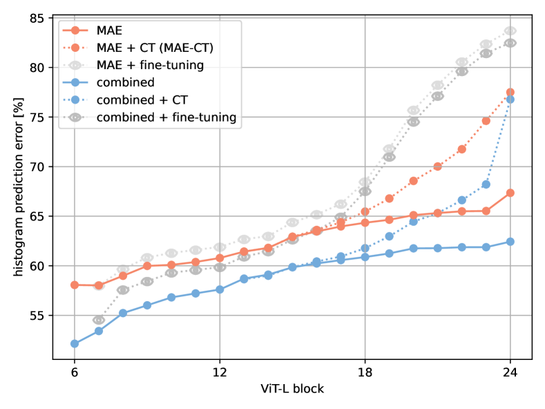
Figure 5: Measuring shortcut learning: Predicting the color histogram of input images from the [CLS] token after different blocks of a ViT-L (higher error is better). Combined pre-training learns shortcut features that can only partially be forgotten via CT or supervised fine-tuning. Sequential training avoids shortcut learning.

Shortcut learning of combined pre-training.

In experiments with combined pre-training, we observe that even with a small NNCLR loss weight $\lambda$ during combined pre-training, the NNCLR loss decreases immediately by about 30% compared to training a detached NNCLR head during combined pre-training. As the encoder does not have a good feature representation at the start of training, this indicates that the NNCLR head steers the encoder to extract basic features which drastically simplify the NNCLR objective. These basic features might be a symptom of shortcut learning [33]. For ID methods, a form of shortcut learning is to learn color statistics of the input image, as two views of the same image likely have a similar color histogram. Following [1] we utilize a prediction task to estimate to what degree the model preserves information about color statistics within the [CLS] token. We train a linear probe to predict the color histograms of the input image. In the combined pre-training, the NNCLR head pushes the encoder towards learning color statistic features (Figure 5). These shortcut features evolve already in early encoder layers of the combined pre-training. While CT is able to partially correct them, they remain more dominant than in the sequentially trained encoder. Not even supervised fine-tuning of all layers — using augmentations based on expert knowledge — can fully mitigate this effect. We describe the color histogram prediction task in Appendix B.1.

Method	$k$	V2	R	Sketch	A
MAE	-	71.7	37.0	24.3	12.3
MAE–CTmin	1	76.4	41.2	27.6	20.5
MAE–CTmin	10	76.6	42.0	28.2	20.8
MAE–CTmin	20	76.5	42.2	28.1	21.4
MAE–CTmin	30	76.5	42.2	28.4	21.5
MAE–CTaug	10	77.9	48.8	35.8	28.2

Table 5: Robustness evaluation with linear classifiers trained on ImageNet. We compare different ViT-L/16 models and report accuracy for multiple values of $k$ in the topk-NN lookup.

Robustness and transfer.

We evaluate the linear probe trained on ImageNet on four transfer learning datasets. Namely, ImageNet-V2 [69], ImageNet-R [40], ImageNet-Sketch [83] and ImageNet-A [41]. In Table 5 we compare the top-1 accuracy of ViT-L/16 models. The results show a small, but overall consistent benefit of the stronger augmentation effect provided by higher values of $k$ in the topk-NN lookup for MAE–CT. MAE–CT_aug is more robust to distribution shifts. The gap between MAE–CT and MAE–CT_aug becomes larger with increase in distribution shift of the datasets (from left to right), but always improves MAE.

Cluster formation.

To demonstrate the differences in clustering we provide results for ImageNet-Dogs15 [13], a subset of ImageNet commonly utilized in the clustering literature. In Figure 6 we show the UMAP [60] embedding of different variations (ViT-L) with their corresponding clustering accuracy. Combined pre-training finds well separated clusters for the classes Norwegian Elkhound, Pug and Maltese Dog. We suspect that these three dog breeds have only small intra-class variations in their characteristics, which makes them easily discernible by low level features. Once contrastive tuning is applied the cluster accuracy improves by a factor of four and also the classes are visually better separated.

\begin{overpic}[width=433.62pt]{figures/large_embedding_imagenet15_dogs_scale_without_titles_2x2_legend_below_larger.pdf} \scriptsize \put(35.0,100.0){MAE: 18.9\%} \put(135.0,100.0){combined pre-training: 32.6\%} \put(35.0,32.0){MAE--CT${}_{min}$: 84.2\%} \put(135.0,32.0){MAE--CT${}_{aug}$: 84.8\%} \end{overpic}

Figure 6: UMAP embeddings of MAE, combined pre-training, MAE–CT_min and MAE–CT_aug with corresponding $k$-means cluster accuracies for ImageNet-Dogs15 (ViT-L). MAE–CT clearly improves the separation of the 15 classes.

Cluster retrieval.

Figure 7 shows the NNs of two $k$-means cluster centroids for ImageNet-Dogs15 of MAE and MAE–CT_min. Inspecting the NNs of the cluster centroid indicates that MAE finds some clusters that correspond to image backgrounds, the first row contains dogs that are located inside and the second row contains dogs that are outside. This is also quantified by the low cluster accuracy w.r.t. the ground truth dog breeds of MAE. MAE reaches a cluster accuracy of 18.7% vs. 94.3% reached by MAE–CT. MAE–CT finds distinct clusters containing mostly images of a single class, shown by the perfect NN retrievals of the classes Basset (third row) and Norwegian Elkhound (fourth row). Note, that the dogs are correctly grouped despite the different background. We provide the full retrieval, confusion matrices and UMAP embeddings in Appendix E.

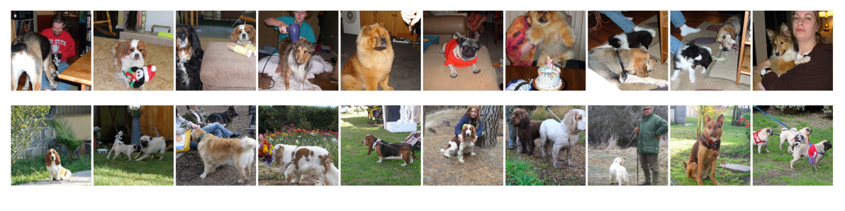
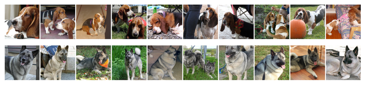
Figure 7: Ten NNs for two $k$-means cluster centers for MAE (upper) and MAE–CT_min (lower). Each row corresponds to one cluster found in the [CLS] token of ViT-H/16 for ImageNet-Dogs15. MAE groups the images into dogs located indoors (first row) and outdoors (second row) depending on the background. MAE–CT finds clusters that correspond to the specific dog breeds.

5 Conclusion

We introduce MAE–CT, a self-supervised approach to combine the strengths of MIM and ID methods. We show that the NNCLR training objective — applied to an already pre-trained MAE model — is capable of creating object-specific clusters in its feature representation which greatly improves representation quality (linear probing, $k$-NN and cluster accuracy) and low-shot classification performance.

We show that our sequential approach preserves the data efficiency of MAE and incorporates the label efficiency of NNCLR while requiring only 10% more compute than MAE pre-training. This allows us to train large ViT models on ImageNet only where our larger models exceed the performance of previous state-of-the-art SSL models.

In contrast to state-of-the-art ID methods, MAE–CT does not rely on hand-crafted image augmentation. This is a very promising result, which can be explained by the data-driven augmentation effect of the NN-lookup, which greatly benefits from representations that already capture image semantics in a structured way.

Appendix

To ensure reproducibility, we list all implementation details regarding training (A) and evaluation (B). We discuss relevant background information (C). We present additional experiments and results (D). Finally, we provide a cluster analysis and show additional qualitative results (E).

Appendix A Training Details

A.1 Implementation details

General

All experiments use the linear lr scaling rule [34] $\textit{lr}=\textit{base lr}\times\textit{batch size}\times\textit{views}/256$ where $\textit{views}=2$ for CT and $\textit{views}=1$ otherwise. Bias and normalization parameters (weights of LayerNorm and BatchNorm layers) are excluded from the weight decay.

In early experiments with float16 we frequently encountered overflows in the attention matrix leading to $\inf$ activations. Therefore, we train all our models in bfloat16 [51] precision. We use FlashAttention [22], which speeds up training by approximately 40/30/20% for ViT-B/L/H respectively.

MAE reimplementation.

In early experiments, we investigated combined pre-training of MAE and NNCLR with a stop gradient operation between encoder and NNCLR head. This effectively corresponds to normal MAE training as the NNCLR head does not influence the MAE pre-training. The only difference is that two views (generated with the augmentations used for MAE pre-training) are used. To account for this difference, we reduce the number of pre-training epochs from 1600 to 800. Additionally, we train with a lower batch size due to memory constraints ($1024$ for ViT-B/L and $512$ for ViT-H). We train a ViT-B/16, ViT-L/16 and ViT-H/16 using this procedure, which we use throughout the main paper. For ViT-H/14 we use the publicly available checkpoint. Table 6 shows that the performance of our re-implementation is nearly identical to the original.

Method	Probing	k-NN
MAEpublic	75.8	60.6
MAEreimpl	75.9	57.6
MAEpublic-CTmin	80.2	77.3
MAEreimpl-CTmin	80.2	77.4

Table 6: Validation of our MAE re-implementation by comparing to the original publicly released checkpoint of a ViT-L/16. For this experiment, CT is done with $k=1$ in the topk-NN lookup.

Algorithm 1 PyTorch-style pseudo-code description of contrastive tuning using an adapted NNCLR head

⬇

# f: ViT encoder .. lower half of the encoder is frozen

# g: projector .. 3 layer MLP, hidden 2048, output 256

# h: predictor .. 2 layer MLP, hidden 4096, output 256

# Q: queue .. shift register of length 65536

# f_m: slow EMA of encoder f .. the model used after CT

# t1: 0.9999 .. momentum parameter of f_m

# g_m: fast EMA of projector g

# t2: 0.99 .. momentum parameter of g_m

# load a minibatch x

for x in loader:

# two randomly augmented versions of x

x1, x2 = augment(x), augment(x)

# encoder forward passes

y1, y2 = f(x1), f(x2)

# predictor path for each y

p1, p2 = h(g(y1)), h(g(y2))

# NN path for each y

z1, z2 = g_m(y1), g_m(y2)

# L2-normalize embeddings

p1, p2 = normalize(p1, dim=1), normalize(p2, dim=1)

z1, z2 = normalize(z1, dim=1), normalize(z2, dim=1)

# topk-NN lookup for each z

nn1 = topk_NN(z1, Q, k)

nn2 = topk_NN(z2, Q, k)

# symmetrised InfoNCE loss

loss = L(nn1, p2)/2 + L(nn2, p1)/2

# optimization step

loss.backward()

optimizer.step()

# shift embeddings z1 into queue Q

update_queue(Q, z1)

# EMA weight updates

f_m = t1 * f_m + (1 - t1) * f

g_m = t2 * g_m + (1 - t2) * g

# topk-NN lookup

def topk_NN(z, Q, k):

similarities = z @ Q.T # matrix multiplication

# calculate list of topk-NN

candidates = similarities.topk(k, dim=1).indices

# uniform sampling

dice = torch.randint(size=(length(Q),), high=k)

idx = candidates[torch.arange(length(Q)),dice]

return Q[idx]

# InfoNCE loss

def L(nn, p, temperature=0.15):

logits = nn @ p.T # matrix multiplication

logits /= temperature # sharpening

labels = torch.arange(p.shape[0])

loss = cross_entropy(logits, labels)

return loss

A.2 Contrastive tuning

ViT architecture.

We follow MAE [37] and use the standard ViT architecture [28]. The ViT projects the input images into patch tokens with a non-overlapping convolutional layer ($\text{stride}=\text{kernel size}$), adds a fixed 2D sine-cosine positional embedding [79] to each patch token, appends an auxiliary [CLS] token and then processes all tokens with a stack of transformer blocks. A transformer block consists of two modules, namely a multi-head self-attention and a 2-layer MLP, which are applied sequentially. Both modules are preceded by a LayerNorm [5] layer and are wrapped with a residual connection [39]. After the last transformer block, a final LayerNorm is applied. We use the [CLS] token of the encoder output as input to the NNCLR head and all evaluations. For ViT-B/16, we use the average of the patch tokens instead of the [CLS] token.

NNCLR architecture.

We follow the design of the original NNCLR head [29] and use a 3-layer MLP as projector and a 2-layer MLP as predictor. Each MLP layer is followed by a BatchNorm [48] except the last predictor layer. Each BatchNorm layer is followed by a ReLU activation except the last projector layer. BatchNorm statistics are calculated per view. To stabilize the entries written into the queue, we apply a fast moving exponential moving average (EMA) [38, 75] to the projector MLP in the topk-NN lookup path.

NNCLR initalization

Before contrastive tuning, we train an NNCLR head with the encoder fully frozen to adjust the NNCLR head to the encoder features using top1-NN lookup, a learning rate of $1e-4$, no EMA in the projector, a temperature $\tau$ of 0.15 and a training duration of $20$ epochs for all model sizes and variants. Other hyperparameters follow the ones from contrastive tuning (Table 7 and 8).

Contrastive tuning.

Algorithm 1 describes the process of contrastive tuning in a PyTorch-like pseudo code. Table 7 and 8 list the hyperparameters used during contrative tuning of MAE–CT_min and MAE–CT_aug, respectively. We find higher values for the temperature $\tau$ to perform best with ViT-H models. We argue that this is caused by the increased capacity of ViT-H and that a higher $\tau$ controls the alignment and uniformity trade-off [84] in the InfoNCE loss. Therefore, a higher $\tau$ slows down the expansion of clusters, as observed in [82]. It is common practice in student-teacher ID methods to use the teacher version of the encoder after training [12]. Thus, we use an exponential moving average (EMA) version of the encoder after contrastive tuning.

MAE–CT	Base	Large	Huge
Epochs	20	20	30
Batch size	1024	1024	512
Optimizer	AdamW [57]
Momentum	$\beta_{1}=0.9,\beta_{2}=0.95$
Learning rate schedule	warmup $\rightarrow$ cosine
Warmup fraction [74]	20 %	20 %	20 %
Encoder
Learning rate	1e-4	1e-4	1e-4
Layer-wise lr decay [19]	0.65	0.65	0.65
Weight decay	0.05	0.05	0.05
Frozen layers	6	12	16
EMA	0.9999	0.9999	0.9999
NNCLR head
Learning rate	1e-4	1e-4	1e-4
Weight decay	1e-5	1e-5	1e-5
Temperature $\tau$	0.15	0.2	0.3
topk-NN $k$	20	20	20
Projector EMA	0.99	0.99	0.995

Table 7: MAE–CT_min hyperparameters.

MAE–CTaug	Base	Large	Huge
Epochs	80	40	40
Batch size	1024	1024	512
Optimizer	AdamW [57]
Momentum	$\beta_{1}=0.9,\beta_{2}=0.95$
Learning rate schedule	warmup $\rightarrow$ cosine
Warmup fraction [74]	20 %	20 %	20 %
Encoder
Learning rate	1e-4	1e-4	1e-4
Layer-wise lr decay [19]	0.65	0.65	0.65
Weight decay	0.05	0.05	0.05
Frozen layers	6	12	16
EMA	0.9999	0.9999	0.9999
NNCLR head
Learning rate	5e-4	5e-4	5e-4
Weight decay	1e-5	1e-5	1e-5
Temperature $\tau$	0.15	0.15	0.35
topk-NN $k$	10	10	30
Projector EMA	0.99	0.99	0.995

Table 8: MAE–CT_aug hyperparameters.

Appendix B Evaluation Details

GPU hours benchmark.

As a comparison between runtimes is often difficult due to differences in code, software and hardware setups we re-implement the compare methods and measure the runtime via a short benchmark run. Benchmarks are conducted on a single A100 40GB PCIe card using pytorch 2.0 with CUDA 11.8 using bfloat16 [51] precision and FlashAttention [22]. We use the largest possible batchsize that is a power of 2. The total number of GPU-hours in Figure 2 is then extrapolated to the number of epochs reported in the original works. As there exists no official implementation for the ViT BatchNorm variants of MoCo v3, we instead report the runtime of the corresponding LayerNorm variant.

Linear probing.

We follow common linear probing protocols and sweep over learning rates [95, 12, 4] and insert a non-affine BatchNorm [48] layer after the fully frozen encoder [26, 37, 3]. Adding a BatchNorm layer does not break the linearity property as it can be absorbed into the linear layer after training. Table 9 lists all parameters.

Config	Value
Epochs	50
Batch size	1024
Optimizer	SGD
Momentum	0.9
Weight decay	0
Learning rate
Peak	$\{0.1,0.09,\dots,0.01\}$
Schedule	warmup $\rightarrow$ cosine
Warmup epochs [34]	5
Augmentations
RandomResizedCrop	$224^{2}$
RandomHorizontalFlip	$p=0.5$

Table 9: Linear probing hyperparameters.

$k$-NN classification.

We also evaluate the feature representation via a weighted $k$-NN classifier following the protocol in DINO [85, 12]. We sweep over different $k$ for every compared method and find $k=10$ to perform well for MAE–CT and MAE–CT_aug. For public checkpoints that do not report $k$-NN accuracies in their original publication, we report the best accuracy over different $k$ for each checkpoint (which is also $k=10$ most of the time). The weighted $k$-NN classifier takes the $k$ training samples with the highest cosine similarity and weights each neighbors class by its cosine similarity with the test sample.

Low-shot classification.

When using 10% of the ImageNet labels, we use the low-shot fine-tuning protocol of I-JEPA [4] to evaluate all compared ID methods (Table 10). We find that all MAE models, all MAE–CT models and the huge models of MAE–CT_aug benefit from more regularization in this setting and therefore use the protocol from the original MAE publication [37], which uses Mixup [93], Cutmix [91], RandomErase [94], DropPath [44] (0.1/0.2/0.3 for ViT-B/L/H) in addition to RandAugment [21] as well as a higher learning rate ($1e-3$). We also consider the MAE fine-tuning protocol for ID methods but find the I-JEPA protocol to perform better.

In the 1% label regime, the protocols of related work vary between fine-tuning [4] and logistic regression [12]. Therefore, we explore logistic regression, the fine-tuning protocol used above and said protocol but with only crop & flip as input augmentations. We find MAE, MAE–CT and MAE–CT_aug to consistently perform better with only crop & flip and report the performance of the best protocol for competing methods. The best performing protocols are: fine-tuning with only crop & flip for MAE, logistic regression for MoCo v3 [18], fine-tuning for iBOT [95] and logistic regression for MSN [3]. Following [9] we use a higher lr ($1e-2$) for MAE with ViT-H/14.

For low-shot evaluations with 1, 2 or 5 labeled samples per class we train a $\text{L}_{2}$-regularized logistic regression using the cyanure package [59] with hyperparameters from previous works [12, 3]. As MAE also benefits from fine-tuning in this low-data regime, we additionally explore full fine-tuning and fine-tuning the last encoder block where we find full fine-tuning to perform best overall. In extreme cases (1 and 2 labels per class with ViT-H) fine-tuning the last block and logistic regression perform slightly better, but we report the full fine-tuning results for consistency.

Config	Value
Epochs	100 (B), 50 (L/H)
Batch size	512
Optimizer	AdamW
Momentum	$\beta_{1}=0.9,\beta_{2}=0.999$
Weight decay	0.05
Learning rate
Peak	3e-5
Schedule	warmup $\rightarrow$ cosine
Warmup epochs [34]	5
Layer-wise lr decay [19]	0.65 (B), 0.75 (L/H)
DropPath [44]	0.0
Label smoothing [74]	0.1
Augmentations
RandomResizedCrop	$224^{2}$
RandomHorizontalFlip	$p=0.5$
RandAugment [21]
num_layers	2
magnitude	9

Table 10: Low-shot fine-tuning hyperparameters.

B.1 Analysis

Color histogram prediction.

We evaluate the amount of information about color statistics by constructing a color histogram prediction task. We calculate the color histograms of an input image, discretize it into $64$ bins and normalize it such that the sum of all bins of each color channel is equal to $1$. This results in a total of $192$ values which we regress with a L1 loss. To make the loss interpretable, we normalize it by dividing it by the average loss on the ImageNet validation set when predicting a uniform distribution (which evaluates to approximately $0.01204$). We call the average over these $192$ normalized loss values ”histogram prediction error”, which can be interpreted as a percentage where $0\%$ is achieved by perfectly predicting the histograms and $100\%$ is the random performance.

We concurrently train $24$ linear probes using the [CLS] tokens of each of the $24$ ViT-L layers with a slightly modified version of the setting described in Table 9. We train for $10$ epochs with $1$ warmup epoch and a learning rate of $0.1$. The encoder is fully frozen throughout training.

Appendix C Background

Instance discrimination (ID).

First, ID methods generate different views of the same image via augmentations. Then, they align the representations of these views in order to obtain representations that are invariant to the transformations that generated the views [76]. A trivial solution for alignment would be a constant representation, which corresponds to a undesired collapse of the representation space to a single point. Representation collapses can be avoided in different ways: (a) contrastive methods [42, 38, 16, 62] rely on a loss that penalizes the similarity to views of other samples, the so-called negatives; (b) teacher-student approaches [35, 12, 17] prevent collapses via an asymmetry between an active student and a teacher; (c) various methods circumvent collapses by constraints that rely on clustering [10, 11] or on invariances [92, 8]. Typically, ID methods learn object-specific representations that are suited to solve downstream classification tasks with few labels.

Masked Image Modeling (MIM).

MIM uses a pre-training task where missing or corrupted parts of the input image have to be reconstructed.

Neither early image in-painting methods [26, 65] nor the adaptation of masked language modeling [25] in computer vision [14] achieved the performance of supervised pre-training. In computer vision, masking methods were revived by the introduction of the Vision Transformer (ViT; [28]). Due to their missing inductive biases, ViTs struggle to learn local features with limited data from supervised training alone [68]. Furthermore, in contrast to convolutional neural networks, the ViT architecture readily enables to mask out patches without introducing undesired artifacts.

Various methods have shown that MIM can improve data efficiency and allows scaling of the model size [7, 37, 87, 6]. On smaller datasets, enhancing contrastive methods by MIM was beneficial [30]. Furthermore, masking the input of the student network has been used to improve the performance of self-distillation methods [95, 3].

Masked self-supervised learning is a very general concept and, therefore, can be applied to various domains such as natural language processing [25], audio processing [45, 52], or computer vision [37, 7, 14, 87]. However, MIM pre-training often does not create features that are suited for downstream tasks such as classification via linear probing or $k$-NN. Typically, downstream tasks require object-focused features while MIM constructs features that are more general and allow to capture the image background. For example, MAEs must also represent the image background to achieve a low reconstruction error. Therefore, adaptation mechanisms such as end-to-end fine-tuning must be applied to achieve optimal performance on downstream tasks. These adaption mechanisms rely on hand-crafted data augmentations [37] such as RandAugment [21], Mixup [93], Cutmix [91], and other regularization techniques [44, 19].

Contrastive and clustering methods.

Clustering-based contrastive methods [54, 10, 11, 12] leverage group information in the form of clusters or prototypes to avoid splitting objects that belong to the same semantic class. Therefore, these methods create object-focused features, which leads to clusters of objects of the same type or even clusters of different views of the same object. However, clustering is prone to early over-generalization by considering an entire cluster as positive examples before a proper discrimination of samples is possible [29]. This phenomenon is known in the deep clustering literature [96], in which a two step approach was shown to avoid over-generalization and trivial solutions [10, 86, 49]. First, pre-training via a self-supervised method learns a suitable representation. Subsequently, samples are clustered starting from the learned representation, thereby the model is fine-tuned to induce better separation. The two step approach can also be implemented as a joint [86] or an alternating [89] procedure.

Similar to our approach, many deep clustering methods use autoencoders for pre-training [96], since they are more generally applicable than contrastive methods. However, their reconstruction objective generates features that do not fit to the discriminative nature of clustering or classification tasks which need object-focused features [31, 61] .

To explain the success of contrastive learning, some work considers the connection between clustering and contrastive methods [64, 71, 36, 15], with recent work [2] pointing to a connection to the $k$-means algorithm [58, 56].

Masked Autoencoder (MAE).

MAE [37] is a popular MIM method, as it enables the training of large ViT models on small datasets with reduced computational cost. During pre-training, a larger ViT model serves as an encoder and a smaller ViT model as a decoder of a Denoising Autoencoder [80]. The latter regresses the missing patches. The high masking ratio shortens the sequence length processed in the encoder, which vastly reduces the computational cost of pre-training. MAEs exhibit strong performance when fine-tuned on computer vison downstream tasks, such as object detection or instance segmentation [55, 43], and also on other modalities such as audio [45] or video [32, 77].

Nearest Neighbor Contrastive Learning (NNCLR).

NNCLR [29] extends the popular contrastive method SimCLR [16] with a Nearest Neighbor (NN) lookup. Instead of calculating the InfoNCE loss between an anchor sample of one view and a positive sample of the other view, the feature vector of the positive sample is replaced by its nearest neighbor from a queue containing feature vectors of previous samples. The queue is implemented via a shift register (similar to MoCo [38]). Additionally, NNCLR adopts the asymmetric head design of BYOL [35].

When restricted to only crop & flip augmentations, NNCLR shows promising resilience to shortcut learning [33]. In an experiment with reduced training duration, NNCLR reports a relative drop of only 2.1% in linear probing performance with ResNet50 [39]. For comparison, other ID methods report a relative drop of $\scriptstyle\sim$13% (BYOL [35]), $\scriptstyle\sim$27% (Barlow Twins [92]), or $\scriptstyle\sim$28% (SimCLR [16]) in performance.

Appendix D Additional Results & Experiments

Hyperparameter sensitivity.

We evaluate the sensitivity of chosen hyperparameters on a ViT-L/16 in Table 11. MAE–CT works well across a range of hyperparameters.

Training epochs	10	gray!1520	30	-
Probing accuracy	79.57	gray!1580.23	80.24	-
$k$-NN accuracy	76.23	gray!1577.36	76.81	-
Trainable layers	6	gray!1512	15	18
Probing accuracy	79.76	gray!1580.23	80.26	80.12
$k$-NN accuracy	76.91	gray!1577.36	77.43	77.49
Encoder EMA	0.0	0.999	gray!150.9999	-
Probing accuracy	80.19	80.21	gray!1580.23	-
$k$-NN accuracy	77.29	77.23	gray!1577.36	-
Temperature $\tau$	0.15	gray!150.2	0.25	-
Probing accuracy	80.12	gray!1580.23	80.12	-
$k$-NN accuracy	77.18	gray!1577.36	77.39	-
$k$-NN lookup $k$	gray!151	10	20	30
Probing accuracy	gray!1580.23	80.16	80.17	80.29
$k$-NN accuracy	gray!1577.36	77.98	77.98	77.90
Projector EMA	0.0	gray!150.99	0.995	0.999
Probing accuracy	80.07	gray!1580.23	80.16	80.13
$k$-NN accuracy	77.13	gray!1577.36	77.31	77.08

Table 11: Sensitivity analysis of MAE–CT with ViT-L/16 using only crop & flip augmentations. Default parameters used in this analysis are marked in gray.

Representations for linear probing.

Following previous works [12, 25], we evaluate the representation of the concatenation of the features from the last $l$ ViT blocks as well as the concatenation of the [CLS] token with the average pooled patch tokens. Table 12 shows that $l=6$ works well for our larger models while the concatenation of the [CLS] and the average of the patch tokens works best for ViT-B/16. We provide these results solely for the sake of completeness and to provide a point of reference. We do not apply this protocol when we compare to other methods.

concat $l$ last layers		1	2	4	6	1†
MAE–CTmin	B/16	73.5	73.2	74.2	74	74.5
MAE–CTmin	L/16	80.2	80.3	80.5	80.8	80.3
MAE–CTmin	H/16	81.5	81.6	81.6	81.6	81.6
MAE–CTaug	B/16	76.9	75.5	76.0	75.9	77.5
MAE–CTaug	L/16	81.5	81.6	81.8	81.8	81.6
MAE–CTaug	H/16	82.2	82.2	82.4	82.3	82.3

Table 12: ImageNet linear probing performance when concatenating the features of the last $l$ layers. ^†: concatenation of the [CLS] token and the average of all patch tokens of the last layer.

Fine-tuning with 100% of the labels.

We show the results for our models in Table 13. As the margin between MAE and MAE–CT is small, we report mean and standard deviation of three seeds. Note that all MAE–CT models start from our own MAE models (as described in Section A.1) which perform slightly worse in the 100% labels benchmark than the original models.

Method	ViT-B/16	ViT-L/16	ViT-H/16
MAEpublic	83.57	85.87 (0.07)	-
MAEreimpl	83.20	85.37 (0.05)	86.50 (0.01)
MAE-CTmin	83.32	85.47 (0.03)	86.59 (0.05)
MAE-CTaug	83.22	85.56 (0.10)	86.57 (0.08)

Table 13: Fine-tuning with 100% of the labels. Parenthesis show the mean and standard deviation of three seeds.

		low-shot evaluations					feature evaluations
Architecture	Method	1 shot	2 shot	5 shot	1%	10%	Linear probing	k-NN
ViT-H/16	MAE	9.0	16.4	55.2	70.0	80.8	78.0	61.1
	MAE-CTmin	53.1	62.3	68.9	75.0	81.2	81.5	79.4
	MAE-CTaug	50.1	60.2	67.7	75.0	81.0	82.2	79.8
ViT-H/14	MAE	7.2	14.1	40.2	72.8	81.2	77.2	58.9
	I-JEPA	34.1	46.3	58.1	73.7	79.5	79.3	71.6
	MAE-CTmin	49.4	59.6	67.4	74.4	81.3	81.2	79.1
	MAE-CTaug	45.5	56.2	64.9	74.0	81.7	82.0	78.9

Table 14: Low-shot and feature evaluations of ViT-H models on ImageNet. The coupling of patch size with mask size of MAE degrades representation quality as analyzed by [43]. Given the inferior starting point of MAE H/14, MAE-CT is still able to leverage the longer sequence length when sufficiently many labels are available (10%), but falls short to the ViT-H/16 model otherwise. We also compare against I-JEPA [4], a recent joint-embedding self-supervised approach.

Results with ViT-H/14.

As analyzed in LongSequencMAE [43], MAE couples the patch size and the mask size since the mask is sampled on a per patch basis. A smaller patch size results in an easier reconstruction task as the average distance between visible patches is reduced. In experiments with ViT-H/14, we find that this coupling leads to a significant degrade in initial representation quality, which manifests in a 2.1% drop in k-NN accuracy and a 0.8% drop in linear probing accuracy (Table 14). Since MAE–CT uses the encoder of a pre-trained MAE, it relies on a good encoder representation. While contrastive tuning can achieve similarly large performance gains on ViT-H/14 when compared to MAE, it only surpasses the ViT-H/16 results on the 10% low-shot benchmark where the number of labels is sufficient to benefit from the increased sequence length. Despite this special interaction in the MAE pre-training, MAE–CT is still able to surpass competing methods using the ViT-H/14 model.

Effective invariance to data augmentation.

We evaluate the average effective invariance [24] against rotations and different color augmentations. For an image $x$ and its augmented version $x_{t}$, [24] defines the effective invariance (EI) as $0$ if the linear classifier predicts different classes and $\sqrt{\hat{p}_{t}\cdot\hat{p}}$ if the predictions agree. $\hat{p}$ denote the predictions for $x$ and $\hat{p}_{t}$ denote the predictions for $x_{t}$. Table 15 shows the average EI for rotations against 90°, 180° and 270° and for color augmentations that include changes in brightness, contrast, hue and saturation. We report the average EI for images in the validation set of ImageNet.

CT increases EI regarding rotations, where using extensive augmentations performs similar to not using them. The hand-crafted image augmentations used in MAE–CT_aug further increase the EI against color augmentations, but also MAE–CT improves over MAE. These results indicate that MAE–CT develops increased robustness against color transformations even though during training the color information in the input is not perturbed.

Method	B/16	L/16	H/16
Effective invariance against rotations
MAE	0.288	0.413	0.450
MAE–CTmin	0.433	0.508	0.530
MAE–CTaug	0.437	0.505	0.529
Effective invariance against color augmentations
MAE	0.481	0.670	0.681
MAE–CTmin	0.544	0.719	0.730
MAE–CTaug	0.714	0.783	0.786

Table 15: Effective Invariance (EI) against multiple transformations. MAE–CT increases the EI compared to MAE, showing that the NN lookup acts as a data-driven augmentation. MAE–CT_aug can further increase the EI against color augmentations due to the hand-crafted augmentations used during contrastive tuning.

Supervised MAE–CT.

To explore the effect of perfect nearest neighbor retrieval, we apply contrastive tuning to a MAE pre-trained ViT-L/16 with an oracle (MAE–CT_oracle) where only samples of the same class are considered as candidates for the nearest neighbor lookup. After 30 epochs of contrastive tuning such a model achieves $83.9\%$ linear probing performance. In Table 16 we compare it against a fully fine-tuned MAE with varying degrees of input augmentations. With only crop & flip augmentation, MAE–CT_oracle outperforms full fine-tuning.

We also validate our fine-tuning pipeline by fine-tuning our MAE pre-trained ViT-L/16 according to the fine-tuning protocol of MAE [37]. We achieve a similar performance of $85.8\%$ compared to $85.9\%$ reported in MAE.

Method	Accuracy
Crop & flip only
MAE–CToracle linear probe	83.9
MAE fine-tuned	83.1
+ Label smoothing [74]	83.7
Additional input augmentations
+ Mixup [93]	84.5
+ Cutmix [91]	84.8
+ RandomErasing [94]	84.8
+ RandAugment [21]	85.8

Table 16: MAE–CT_oracle with linear probing compared to fine-tuning a MAE on ImageNet with a ViT-L/16 as encoder. When only crop & flip is used, MAE–CT_oracle performs better with linear probing than a fully fine-tuned MAE. Rows starting with ”+” add an additional component to the setting of the previous row.

Extended results.

Table 17 on the next page presents an extended version of the linear probing and $k$-NN result tables of the main paper. We include results from models that use smaller patches or a higher input resolution.

Method	Architecture	Epochs	GV/LV/T	Mask ratio	Probe	$k$-NN
minimal image augmentations
SimMIM [87]	ViT-B/16	800	1	0.5	56.7	-
MAE [37]	ViT-B/16	1600	1	0.75	68.0	50.0
MAE [37]	ViT-L/16	1600	1	0.75	76.0	60.6
MAE [37]	ViT-H/14	1600	1	0.75	77.2	58.9
MAE (reimpl.)	ViT-B/16	800	2	0.75	66.7	51.1
MAE (reimpl.)	ViT-L/16	800	2	0.75	75.9	57.6
MAE (reimpl.)	ViT-H/16	800	2	0.75	78.0	61.1
I-JEPA [4]	ViT-B/16	600	1* / 4* / 1	*	72.9	-
I-JEPA [4]	ViT-L/16	600	1* / 4* / 1	*	77.5	-
I-JEPA [4]	ViT-H/14	300	1* / 4* / 1	*	79.3	71.6
I-JEPA [4]	ViT-H/16448	300	1* / 4* / 1	*	81.1	70.1
MAE–CTmin	ViT-B/16	800; 20	2	0.75; 0	73.5	64.1
MAE–CTmin	ViT-L/16	800; 20	2	0.75; 0	80.2	78.0
MAE–CTmin	ViT-H/16	800; 30	2	0.75; 0	81.5	79.4
extensive image augmentations
NNCLR [29]	ViT-B/16	1000	2	-	76.5	-
MoCo v3 [18]	ViT-B/16	600	2	-	76.7	72.6
MoCo v3 [18]	ViT-L/16	300	2	-	77.6	-
MoCo v3 [18]	ViT-L/7-BN	300	2	-	81.0	-
MoCo v3 [18]	ViT-H/14	300	2	-	78.1	-
MoCo v3 [18]	ViT-H/14-BN	300	2	-	79.1	-
DINO [12]	ViT-S/8	400	2 / 10 / 2	79.7	78.3
DINO [12]	ViT-B/16	400	2 / 10 / 2	78.2	76.1
DINO [12]	ViT-B/8	400	2 / 10 / 2	-	80.1	77.4
iBOT [95]	ViT-B/16	400	2 / 10 / 2	$\approx$ 0.15†	79.5	77.1
iBOT [95]	ViT-L/16	250	2 / 10 / 2	$\approx$ 0.15†	81.0	78.0
MSN [3]	ViT-L/7	200	1 / 10 / 1	0.7	80.7	-
CMAE [46]	ViT-B/16	1600	1 / - / 1	0.75	73.9	-
Layer Grafting [50]	ViT-B/16	1600; 300	1; 2 / - / - ; 2	0.75; 0	77.9	75.4
Layer Grafting [50]	ViT-L/16	1600; 300	1; 2 / - / - ; 2	0.75; 0	81.0	77.3
MAE–CTaug	ViT-B/16	800; 80	2	0.75; 0	76.9	73.4
MAE–CTaug	ViT-L/16	800; 40	2	0.75; 0	81.5	79.1
MAE–CTaug	ViT-H/16	800; 40	2	0.75; 0	82.2	79.8

Table 17: Comparison of linear probing and $k$-NN accuracies, including results of methods that use smaller patches or higher resolutions. Furthermore, training details are listed. Namely, the training duration, the number of global views (GV), the number of local views (LV, multi-crop), the number of teacher forward passes (T) and the masking ratio.
* I-JEPA uses a multiblock-masking scheme, consisting of one context block and four target blocks (no encoder forward pass) per sample. Thus the effective masking ratio is a result of the size of the context block, the sizes of the target blocks and the overlap between them.
† iBOT applies masking only half of the time during training. If masking is applied the masking ratio is sampled between 0.1 and 0.5.

Appendix E Cluster Analysis

Experiment details.

The clustering performance metrics in Table 4 of the main paper are obtained by applying $k$-means to the [CLS] token in the last layer of each ViT encoder. Only for MAE–CT and MAE–CT_aug with ViT-B we use the average over the patch tokens of the last encoder layer for clustering. For each method we encoded the validation set of ImageNet and standardized the embedding using its mean and standard deviation. The standardized embedding is then clustered 100 times with mini-batch $k$-means, a mini-batch variant of $k$-means that scales better with larger data sets [72]. From the 100 runs we selected the one with the lowest $k$-means loss and calculated the cluster accuracy [90] w.r.t. the 1000 ground truth ImageNet classes. For ImageNet-Dogs15 [13] we performed the same procedure with the number of clusters $k=15$.

Quantitative results.

In Table 18 we show for completeness the best (w.r.t. the lowest $k$-means loss) clustering performance for ImageNet and in Table 19 we report the average results. For ImageNet-Dogs15 we report the best results in Table 20 and average results in Table 21. In addition to the cluster accuracy (ACC) results presented in the main paper we report the commonly used clustering metrics Normalized Mutual Information (NMI; [63]), Adjusted Mutual Information (AMI; [63]) and Adjusted Rand Index (ARI; [47]) as well. ACC, NMI, AMI and ARI are all multiplied by 100, so they range between 0 and 100, where higher values indicate a better match with the ground truth labels. The ACC standard deviations over the 100 runs are small for ImageNet, ranging from 0.2% to 0.7% and higher for ImageNet-Dogs15, ranging from 0.6% to 4.3%.

Qualitative results.

In Figure 8 we show the UMAP [60] plots for the [CLS] token embedding of ImageNet-Dogs15 of MAE vs. MAE–CT_min for ViT-H/16. We see that the cluster structure is much more visible for MAE–CT_min. Figure 9 shows the corresponding confusion matrices, where clusters are matched to the ground truth classes using a variant of the Hungarian algorithm [20]. In Figure 10 we show the corresponding cluster retrievals for MAE vs. MAE–CT_min where we can see again that the nearest neighbors of $k$-means cluster centers discovered by MAE–CT_min are focusing more on the different dog breeds than on the background as in MAE. Additionally, Figure 11 shows three samples of ImageNet and the nearest neighbors for MAE, MAE–CT_min and MAE–CT_aug, respectively.

\begin{overpic}[width=433.62pt]{figures/huge_embedding_imagenet15_dogs.pdf} \scriptsize \put(30.0,120.0){MAE: 18.7\%} \put(130.0,120.0){MAE--CT${}_{min}$: 94.3\%} \end{overpic}

Figure 8: Visualization of UMAP embeddings from the [CLS] token of ViT-H/16 over MAE and MAE–CT_min with corresponding $k$-means cluster accuracies (w.r.t. lowest $k$-means loss) for ImageNet-Dogs15. MAE–CT_min clearly improves the separation of the 15 classes.

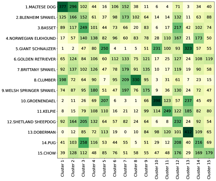
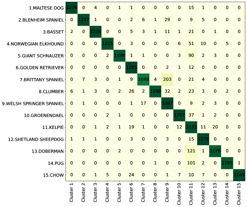
Figure 9: Confusion matrices w.r.t. the clustering result with lowest $k$-means loss for MAE (upper) with 18.7% cluster accuracy and MAE–CT_min (lower) with 94.3% for ViT-H/16. MAE–CT_min discovers clusters that correspond well to the ground truth dog breeds.

	ViT-B/16				ViT-L/16				ViT-H/16
Method	ACC	NMI	AMI	ARI	ACC	NMI	AMI	ARI	ACC	NMI	AMI	ARI
minimal image augmentations
MAE (reimpl.)	13.8	51.4	20.7	4.4	14.3	51.9	22.8	4.6	11.1	48.2	17.1	2.9
MAE–CTmin	35.3	68.2	45.8	19.7	54.9	80.6	66.8	34.5	58.0	81.8	69.3	36.8
extensive image augmentations
Moco v3	43.0	73.0	55.5	23.1	-	-	-	-	-	-	-	-
DINO	48.0	77.9	63.2	31.2	-	-	-	-	-	-	-	-
MSN	54.2	79.9	66.6	30.2	45.4	76.2	63.2	19.5	-	-	-	-
iBOT	50.0	79.1	64.9	32.6	52.0	80.5	66.8	35.0	-	-	-	-
MAE–CTaug	46.2	76.0	59.0	29.8	56.9	81.7	68.4	40.5	54.8	81.1	67.6	38.9

Table 18: Best cluster performance of $k$-means (w.r.t. lowest $k$-means loss) over 100 runs for ImageNet validation set.

	ViT-B/16				ViT-L/16				ViT-H/16
Method	ACC	NMI	AMI	ARI	ACC	NMI	AMI	ARI	ACC	NMI	AMI	ARI
minimal image augmentations
MAE (reimpl.)	13.5	51.0	20.8	4.3	13.9	51.2	22.9	4.5	10.6	47.5	17.0	2.7
MAE–CTmin	35.0	68.0	45.4	19.5	54.1	80.6	66.9	34.7	57.1	81.7	69.2	35.6
extensive image augmentations
Moco v3	41.5	72.4	55.2	21.2	-	-	-	-	-	-	-	-
DINO	46.5	77.3	62.7	29.0	-	-	-	-	-	-	-	-
MSN	52.7	79.4	65.9	28.8	43.6	75.6	62.7	18.6	-	-	-	-
iBOT	49.2	78.7	64.6	31.6	51.2	80.1	66.4	34.1	-	-	-	-
MAE–CTaug	45.3	75.7	58.8	28.6	55.6	81.4	68.0	39.4	54.7	80.8	67.3	37.8

Table 19: Average cluster performance of $k$-means over 100 runs for ImageNet validation set.

	ViT-B/16				ViT-L/16				ViT-H/16
Method	ACC	NMI	AMI	ARI	ACC	NMI	AMI	ARI	ACC	NMI	AMI	ARI
minimal image augmentations
MAE (reimpl.)	16.0	8.1	7.9	3.2	18.9	12.8	12.6	5.2	18.7	11.7	11.6	4.7
MAE–CTmin	70.8	69.1	69.0	54.3	84.2	85.6	85.6	76.4	94.3	90.4	90.4	87.9
extensive image augmentations
Moco v3	72.7	71.9	71.8	59.3	-	-	-	-	-	-	-	-
DINO	79.0	78.9	78.9	69.4	-	-	-	-	-	-	-	-
MSN	81.0	83.6	83.6	73.7	83.3	84.2	84.2	75.9	-	-	-	-
iBOT	77.2	78.8	78.8	68.5	69.4	72.8	72.8	59.9	-	-	-	-
MAE–CTaug	78.1	77.4	77.3	65.0	84.8	87.8	87.8	81.1	83.7	86.5	86.4	79.3

Table 20: Best cluster performance of $k$-means (w.r.t. lowest $k$-means loss) over 100 runs for ImageNet-Dogs15.

	ViT-B/16				ViT-L/16				ViT-H/16
Method	ACC	NMI	AMI	ARI	ACC	NMI	AMI	ARI	ACC	NMI	AMI	ARI
minimal image augmentations
MAE (reimpl.)	15.7	8.5	8.3	3.3	18.5	12.3	12.1	5.2	17.6	11.7	11.5	4.8
MAE–CTmin	67.9	69.2	69.2	53.5	79.9	83.4	83.4	72.7	87.4	88.2	88.2	82.1
extensive image augmentations
Moco v3	66.7	68.8	68.8	54.2	-	-	-	-	-	-	-	-
DINO	71.4	75.2	75.2	62.2	-	-	-	-	-	-	-	-
MSN	79.7	82.4	82.3	72.2	79.5	82.9	82.9	72.5	-	-	-	-
iBOT	75.2	78.6	78.6	66.9	64.8	70.5	70.4	55.4	-	-	-	-
MAE–CTaug	71.7	74.7	74.7	60.3	84.7	86.5	86.4	79.1	83.2	86.0	86.0	78.2

Table 21: Average cluster performance of $k$-means over 100 runs for ImageNet-Dogs15.

\begin{overpic}[width=210.30595pt]{figures/mae_baseline_cluster_retrieval_with_larger_titles.pdf} \scriptsize \put(248.0,421.0){C1} \put(248.0,392.0){C2} \put(248.0,363.0){C3} \put(248.0,334.0){C4} \put(248.0,305.0){C5} \put(248.0,276.0){C6} \put(248.0,247.0){C7} \put(248.0,218.0){C8} \put(248.0,189.0){C9} \put(248.0,160.0){C10} \put(248.0,131.0){C11} \put(248.0,98.0){C12} \put(248.0,72.0){C13} \put(248.0,42.0){C14} \put(248.0,15.0){C15} \end{overpic}

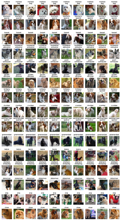
Figure 10: Cluster retrieval: Ten nearest neighbors per $k$-means cluster center for MAE (left) and MAE–CT_min (right). Each row corresponds to one cluster (C1 to C15) found in the [CLS] token embedding of ViT-H/16 for Imagenet-Dogs15. MAE clusters correspond more to background and surface characteristics like color, while MAE–CT_min found clusters that correspond to the 15 dog breeds. The mapping from each cluster to dog breed for MAE–CT_min can be found in the confusion matrix in Figure 9, e.g. the first row is cluster $1$ (C1) and corresponds to the class maltese dog. Additionally, the ground truth label is shown on top of each image (best viewed with zooming in).

Figure 11: Nearest neighbor retrieval: Nearest neighbors for three different sample images (first column) for MAE, MAE–CT and MAE–CT_aug. The NNs are computed by calculating the [CLS] token embedding of a ViT-H for all images in the ImageNet validation set and searching for the most similar embeddings in terms of cosine similarity. The first and the second example images (partridge and strawberry) show that the NNs of the MAE are similar in the context in which the image was taken but almost never contain the correct class. However, the NNs of the MAE–CT and the MAE–CT_aug are images of the same class as the example images. The third sample image is labeled as viaduct, but the image clearly also contains a steam locomotive. The NNs of the MAE all belong to different classes, which shows that the MAE has not captured the semantics of a viaduct or a steam locomotive. The NNs of the MAE–CT and the MAE–CT_aug are all of the same class, but it is either the steam locomotive or the viaduct. All NNs of MAE–CT_aug are images of other viaducts recognizable by their characteristic shape, showing that the augmentations of MAE–CT_aug result in a representation that focuses more on shapes and less on characteristic colors, like black locomotives.

References

- [1] Sravanti Addepalli, Kaushal Bhogale, Priyam Dey, and R. Venkatesh Babu. Towards efficient and effective self-supervised learning of visual representations. In European Conference on Computer Vision, ECCV 2022, volume 13691, pages 523–538, 2022.
- [2] Mido Assran, Randall Balestriero, Quentin Duval, Florian Bordes, Ishan Misra, Piotr Bojanowski, Pascal Vincent, Michael G. Rabbat, and Nicolas Ballas. The hidden uniform cluster prior in self-supervised learning. In The Eleventh International Conference on Learning Representations, ICLR, 2023.
- [3] Mahmoud Assran, Mathilde Caron, Ishan Misra, Piotr Bojanowski, Florian Bordes, Pascal Vincent, Armand Joulin, Mike Rabbat, and Nicolas Ballas. Masked siamese networks for label-efficient learning. In European Conference on Computer Vision, ECCV, volume 13691, pages 456–473, 2022.
- [4] Mahmoud Assran, Quentin Duval, Ishan Misra, Piotr Bojanowski, Pascal Vincent, Michael G. Rabbat, Yann LeCun, and Nicolas Ballas. Self-supervised learning from images with a joint-embedding predictive architecture. In Proceedings of the IEEE/CVF Conference on Computer Vision and Pattern Recognition, CVPR, 2023.
- [5] Lei Jimmy Ba, Jamie Ryan Kiros, and Geoffrey E. Hinton. Layer normalization. CoRR, abs/1607.06450, 2016.
- [6] Alexei Baevski, Wei-Ning Hsu, Qiantong Xu, Arun Babu, Jiatao Gu, and Michael Auli. data2vec: A general framework for self-supervised learning in speech, vision and language. In Proceedings of the 37th International Conference on Machine Learning, ICML, volume 162, pages 1298–1312, 2022.
- [7] Hangbo Bao, Li Dong, Songhao Piao, and Furu Wei. Beit: BERT pre-training of image transformers. In The Tenth International Conference on Learning Representations, ICLR, 2022.
- [8] Adrien Bardes, Jean Ponce, and Yann LeCun. Vicreg: Variance-invariance-covariance regularization for self-supervised learning. In The Tenth International Conference on Learning Representations, ICLR, 2022.
- [9] Zhaowei Cai, Avinash Ravichandran, Paolo Favaro, Manchen Wang, Davide Modolo, Rahul Bhotika, Zhuowen Tu, and Stefano Soatto. Semi-supervised vision transformers at scale. In Advances in Neural Information Processing Systems 33, NeurIPS, 2022.
- [10] Mathilde Caron, Piotr Bojanowski, Armand Joulin, and Matthijs Douze. Deep clustering for unsupervised learning of visual features. In European Conference on Computer Vision, ECCV, volume 11218, pages 139–156, 2018.
- [11] Mathilde Caron, Ishan Misra, Julien Mairal, Priya Goyal, Piotr Bojanowski, and Armand Joulin. Unsupervised learning of visual features by contrasting cluster assignments. In Advances in Neural Information Processing Systems 33, NeurIPS, 2020.
- [12] Mathilde Caron, Hugo Touvron, Ishan Misra, Hervé Jégou, Julien Mairal, Piotr Bojanowski, and Armand Joulin. Emerging properties in self-supervised vision transformers. In IEEE/CVF International Conference on Computer Vision, ICCV, pages 9630–9640, 2021.
- [13] Jianlong Chang, Lingfeng Wang, Gaofeng Meng, Shiming Xiang, and Chunhong Pan. Deep adaptive image clustering. In IEEE International Conference on Computer Vision, ICCV, pages 5880–5888, 2017.
- [14] Mark Chen, Alec Radford, Rewon Child, Jeffrey Wu, Heewoo Jun, David Luan, and Ilya Sutskever. Generative pretraining from pixels. In Proceedings of the 35th International Conference on Machine Learning, ICML, volume 119, pages 1691–1703, 2020.
- [15] Mayee F. Chen, Daniel Y. Fu, Avanika Narayan, Michael Zhang, Zhao Song, Kayvon Fatahalian, and Christopher Ré. Perfectly balanced: Improving transfer and robustness of supervised contrastive learning. In Proceedings of the 37th International Conference on Machine Learning, ICML, volume 162, pages 3090–3122, 2022.
- [16] Ting Chen, Simon Kornblith, Mohammad Norouzi, and Geoffrey E. Hinton. A simple framework for contrastive learning of visual representations. In Proceedings of the 37th International Conference on Machine Learning, ICML, volume 119, pages 1597–1607, 2020.
- [17] Xinlei Chen and Kaiming He. Exploring simple siamese representation learning. In Proceedings of the IEEE/CVF Conference on Computer Vision and Pattern Recognition, CVPR, pages 15750–15758, 2021.
- [18] Xinlei Chen, Saining Xie, and Kaiming He. An empirical study of training self-supervised vision transformers. In IEEE/CVF International Conference on Computer Vision ICCV, pages 9620–9629, 2021.
- [19] Kevin Clark, Minh-Thang Luong, Quoc V. Le, and Christopher D. Manning. ELECTRA: pre-training text encoders as discriminators rather than generators. In 8th International Conference on Learning Representations, ICLR, 2020.
- [20] David Frederic Crouse. On implementing 2d rectangular assignment algorithms. IEEE Trans. Aerosp. Electron. Syst., 52(4):1679–1696, 2016.
- [21] Ekin Dogus Cubuk, Barret Zoph, Jonathon Shlens, and Quoc Le. Randaugment: Practical automated data augmentation with a reduced search space. In Advances in Neural Information Processing Systems 33, NeurIPS, 2020.
- [22] Tri Dao, Daniel Y. Fu, Stefano Ermon, Atri Rudra, and Christopher Ré. Flashattention: Fast and memory-efficient exact attention with io-awareness. In Advances in Neural Information Processing Systems 35, NeurIPS, 2022.
- [23] Jia Deng, Wei Dong, Richard Socher, Li-Jia Li, Kai Li, and Li Fei-Fei. Imagenet: A large-scale hierarchical image database. In IEEE Computer Society Conference on Computer Vision and Pattern Recognition, CVPR, pages 248–255, 2009.
- [24] Weijian Deng, Stephen Gould, and Liang Zheng. On the strong correlation between model invariance and generalization. In Advances in Neural Information Processing Systems 35, NeurIPS, 2022.
- [25] Jacob Devlin, Ming-Wei Chang, Kenton Lee, and Kristina Toutanova. BERT: pre-training of deep bidirectional transformers for language understanding. In Proceedings of the 2019 Conference of the North American Chapter of the Association for Computational Linguistics: Human Language Technologies, NAACL-HLT), pages 4171–4186, 2019.
- [26] Carl Doersch, Abhinav Gupta, and Alexei A. Efros. Unsupervised visual representation learning by context prediction. In IEEE International Conference on Computer Vision, ICCV, pages 1422–1430, 2015.
- [27] Xiaoyi Dong, Jianmin Bao, Ting Zhang, Dongdong Chen, Weiming Zhang, Lu Yuan, Dong Chen, Fang Wen, and Nenghai Yu. Bootstrapped masked autoencoders for vision BERT pretraining. In European Conference on Computer Vision, ECCV, volume 13690, pages 247–264, 2022.
- [28] Alexey Dosovitskiy, Lucas Beyer, Alexander Kolesnikov, Dirk Weissenborn, Xiaohua Zhai, Thomas Unterthiner, Mostafa Dehghani, Matthias Minderer, Georg Heigold, Sylvain Gelly, Jakob Uszkoreit, and Neil Houlsby. An image is worth 16x16 words: Transformers for image recognition at scale. In 9th International Conference on Learning Representations, ICLR, 2021.
- [29] Debidatta Dwibedi, Yusuf Aytar, Jonathan Tompson, Pierre Sermanet, and Andrew Zisserman. With a little help from my friends: Nearest-neighbor contrastive learning of visual representations. In IEEE/CVF International Conference on Computer Vision ICCV, pages 9568–9577, 2021.
- [30] Alaaeldin El-Nouby, Gautier Izacard, Hugo Touvron, Ivan Laptev, Hervé Jégou, and Edouard Grave. Are large-scale datasets necessary for self-supervised pre-training? CoRR, abs/2112.10740, 2021.
- [31] Baruch Epstein and Ron Meir. Generalization bounds for unsupervised and semi-supervised learning with autoencoders. CoRR, abs/1902.01449, 2019.
- [32] Christoph Feichtenhofer, Haoqi Fan, Yanghao Li, and Kaiming He. Masked autoencoders as spatiotemporal learners. In Advances in Neural Information Processing Systems 35, NeurIPS, 2022.
- [33] Robert Geirhos, Jörn-Henrik Jacobsen, Claudio Michaelis, Richard S. Zemel, Wieland Brendel, Matthias Bethge, and Felix A. Wichmann. Shortcut learning in deep neural networks. Nat. Mach. Intell., 2(11):665–673, 2020.
- [34] Priya Goyal, Piotr Dollár, Ross B. Girshick, Pieter Noordhuis, Lukasz Wesolowski, Aapo Kyrola, Andrew Tulloch, Yangqing Jia, and Kaiming He. Accurate, large minibatch SGD: training imagenet in 1 hour. CoRR, abs/1706.02677, 2017.
- [35] Jean-Bastien Grill, Florian Strub, Florent Altché, Corentin Tallec, Pierre H. Richemond, Elena Buchatskaya, Carl Doersch, Bernardo Ávila Pires, Zhaohan Guo, Mohammad Gheshlaghi Azar, Bilal Piot, Koray Kavukcuoglu, Rémi Munos, and Michal Valko. Bootstrap your own latent - A new approach to self-supervised learning. In Advances in Neural Information Processing Systems 33, NeurIPS, 2020.
- [36] Jeff Z. HaoChen and Tengyu Ma. A theoretical study of inductive biases in contrastive learning. In The Eleventh International Conference on Learning Representations, ICLR, 2023.
- [37] Kaiming He, Xinlei Chen, Saining Xie, Yanghao Li, Piotr Dollár, and Ross B. Girshick. Masked autoencoders are scalable vision learners. In Proceedings of the IEEE/CVF Conference on Computer Vision and Pattern Recognition, CVPR, pages 15979–15988, 2022.
- [38] Kaiming He, Haoqi Fan, Yuxin Wu, Saining Xie, and Ross B. Girshick. Momentum contrast for unsupervised visual representation learning. In Proceedings of the IEEE/CVF Conference on Computer Vision and Pattern Recognition, CVPR, pages 9726–9735, 2020.
- [39] Kaiming He, Xiangyu Zhang, Shaoqing Ren, and Jian Sun. Deep residual learning for image recognition. In IEEE Conference on Computer Vision and Pattern Recognition, CVPR, pages 770–778, 2016.
- [40] Dan Hendrycks, Steven Basart, Norman Mu, Saurav Kadavath, Frank Wang, Evan Dorundo, Rahul Desai, Tyler Zhu, Samyak Parajuli, Mike Guo, Dawn Song, Jacob Steinhardt, and Justin Gilmer. The many faces of robustness: A critical analysis of out-of-distribution generalization. In IEEE/CVF International Conference on Computer Vision, ICCV, pages 8320–8329, 2021.
- [41] Dan Hendrycks, Kevin Zhao, Steven Basart, Jacob Steinhardt, and Dawn Song. Natural adversarial examples. In IEEE/CVF Conference on Computer Vision and Pattern Recognition, CVPR, pages 15262–15271, 2021.
- [42] R. Devon Hjelm, Alex Fedorov, Samuel Lavoie-Marchildon, Karan Grewal, Philip Bachman, Adam Trischler, and Yoshua Bengio. Learning deep representations by mutual information estimation and maximization. In The seventh International Conference on Learning Representations, ICLR, 2019.
- [43] Ronghang Hu, Shoubhik Debnath, Saining Xie, and Xinlei Chen. Exploring long-sequence masked autoencoders. CoRR, abs/2210.07224, 2022.
- [44] Gao Huang, Yu Sun, Zhuang Liu, Daniel Sedra, and Kilian Q. Weinberger. Deep networks with stochastic depth. In European Conference on Computer Vision, ECCV, volume 9908 of Lecture Notes in Computer Science, pages 646–661. Springer, 2016.
- [45] Po-Yao Huang, Hu Xu, Juncheng Li, Alexei Baevski, Michael Auli, Wojciech Galuba, Florian Metze, and Christoph Feichtenhofer. Masked autoencoders that listen. In Advances in Neural Information Processing Systems 35, NeurIPS, 2022.
- [46] Zhicheng Huang, Xiaojie Jin, Chengze Lu, Qibin Hou, Ming-Ming Cheng, Dongmei Fu, Xiaohui Shen, and Jiashi Feng. Contrastive masked autoencoders are stronger vision learners. CoRR, abs/2207.13532, 2022.
- [47] Lawrence Hubert and Phipps Arabie. Comparing partitions. Journal of classification, 2(1):193–218, 1985.
- [48] Sergey Ioffe and Christian Szegedy. Batch normalization: Accelerating deep network training by reducing internal covariate shift. In Proceedings of the 32nd International Conference on Machine Learning, ICML, volume 37, pages 448–456, 2015.
- [49] Xu Ji, Andrea Vedaldi, and João F. Henriques. Invariant information clustering for unsupervised image classification and segmentation. In IEEE/CVF International Conference on Computer Vision, ICCV, pages 9864–9873, 2019.
- [50] Ziyu Jiang, Yinpeng Chen, Mengchen Liu, Dongdong Chen, Xiyang Dai, Lu Yuan, Zicheng Liu, and Zhangyang Wang. Layer grafted pre-training: Bridging contrastive learning and masked image modeling for label-efficient representations. In The Eleventh International Conference on Learning Representations, ICLR, 2023.
- [51] Dhiraj D. Kalamkar, Dheevatsa Mudigere, Naveen Mellempudi, Dipankar Das, Kunal Banerjee, Sasikanth Avancha, Dharma Teja Vooturi, Nataraj Jammalamadaka, Jianyu Huang, Hector Yuen, Jiyan Yang, Jongsoo Park, Alexander Heinecke, Evangelos Georganas, Sudarshan Srinivasan, Abhisek Kundu, Misha Smelyanskiy, Bharat Kaul, and Pradeep Dubey. A study of BFLOAT16 for deep learning training. CoRR, abs/1905.12322, 2019.
- [52] Khaled Koutini, Jan Schlüter, Hamid Eghbal-zadeh, and Gerhard Widmer. Efficient training of audio transformers with patchout. In 23rd Annual Conference of the International Speech Communication Association, Interspeech, pages 2753–2757, 2022.
- [53] Samuli Laine and Timo Aila. Temporal ensembling for semi-supervised learning. In 5th International Conference on Learning Representations, ICLR 2017, 2017.
- [54] Yunfan Li, Peng Hu, Jerry Zitao Liu, Dezhong Peng, Joey Tianyi Zhou, and Xi Peng. Contrastive clustering. In Thirty-Fifth AAAI Conference on Artificial Intelligence, AAAI, pages 8547–8555, 2021.
- [55] Yanghao Li, Saining Xie, Xinlei Chen, Piotr Dollár, Kaiming He, and Ross B. Girshick. Benchmarking detection transfer learning with vision transformers. CoRR, abs/2111.11429, 2021.
- [56] Stuart P. Lloyd. Least squares quantization in PCM. IEEETransactions on Information Theory, 28(2):129–136, 1982.
- [57] Ilya Loshchilov and Frank Hutter. Decoupled weight decay regularization. In The 7th International Conference on Learning Representations, ICLR, 2019.
- [58] James B. MacQueen. Some methods for classification and analysis of multivariate observations. In Proc. 5th Berkeley Symposium on Math., Stat., and Prob, page 281, 1965.
- [59] Julien Mairal. Cyanure: An open-source toolbox for empirical risk minimization for python, c++, and soon more. CoRR, abs/1912.08165, 2019.
- [60] Leland McInnes, John Healy, Nathaniel Saul, and Lukas Großberger. UMAP: uniform manifold approximation and projection. J. Open Source Softw., 3(29):861, 2018.
- [61] Lukas Miklautz, Lena G. M. Bauer, Dominik Mautz, Sebastian Tschiatschek, Christian Böhm, and Claudia Plant. Details (don’t) matter: Isolating cluster information in deep embedded spaces. In Proceedings of the Thirtieth International Joint Conference on Artificial Intelligence, IJCAI, pages 2826–2832, 2021.
- [62] Ishan Misra and Laurens van der Maaten. Self-supervised learning of pretext-invariant representations. In IEEE/CVF Conference on Computer Vision and Pattern Recognition, CVPR, pages 6706–6716, 2020.
- [63] Xuan Vinh Nguyen, Julien Epps, and James Bailey. Information theoretic measures for clusterings comparison: Variants, properties, normalization and correction for chance. Journal of Machine Learning Research, JMLR, 11:2837–2854, 2010.
- [64] Advait Parulekar, Liam Collins, Karthikeyan Shanmugam, Aryan Mokhtari, and Sanjay Shakkottai. Infonce loss provably learns cluster-preserving representations. CoRR, abs/2302.07920, 2023.
- [65] Deepak Pathak, Philipp Krähenbühl, Jeff Donahue, Trevor Darrell, and Alexei A. Efros. Context encoders: Feature learning by inpainting. In IEEE Conference on Computer Vision and Pattern Recognition, CVPR, pages 2536–2544, 2016.
- [66] F. Pedregosa, G. Varoquaux, A. Gramfort, V. Michel, B. Thirion, O. Grisel, M. Blondel, P. Prettenhofer, R. Weiss, V. Dubourg, J. Vanderplas, A. Passos, D. Cournapeau, M. Brucher, M. Perrot, and E. Duchesnay. Scikit-learn: Machine learning in Python. Journal of Machine Learning Research, 12:2825–2830, 2011.
- [67] Trung Pham, Chaoning Zhang, Axi Niu, Kang Zhang, and Chang D. Yoo. On the pros and cons of momentum encoder in self-supervised visual representation learning. CoRR, abs/2208.05744, 2022.
- [68] Maithra Raghu, Thomas Unterthiner, Simon Kornblith, Chiyuan Zhang, and Alexey Dosovitskiy. Do vision transformers see like convolutional neural networks? In Advances in Neural Information Processing Systems 34, NeurIPS, pages 12116–12128, 2021.
- [69] Benjamin Recht, Rebecca Roelofs, Ludwig Schmidt, and Vaishaal Shankar. Do imagenet classifiers generalize to imagenet? In Proceedings of the 36th International Conference on Machine Learning, ICML, volume 97 of Proceedings of Machine Learning Research, pages 5389–5400, 2019.
- [70] Peter J. Rousseeuw. Silhouettes: a graphical aid to the interpretation and validation of cluster analysis. Journal of computational and applied mathematics, 20:53–65, 1987.
- [71] Nikunj Saunshi, Orestis Plevrakis, Sanjeev Arora, Mikhail Khodak, and Hrishikesh Khandeparkar. A theoretical analysis of contrastive unsupervised representation learning. In Proceedings of the 36th International Conference on Machine Learning, ICML, volume 97, pages 5628–5637, 2019.
- [72] D. Sculley. Web-scale k-means clustering. In Michael Rappa, Paul Jones, Juliana Freire, and Soumen Chakrabarti, editors, Proceedings of the 19th International Conference on World Wide Web, WWW, pages 1177–1178, 2010.
- [73] Mannat Singh, Quentin Duval, Kalyan Vasudev Alwala, Haoqi Fan, Vaibhav Aggarwal, Aaron Adcock, Armand Joulin, Piotr Dollár, Christoph Feichtenhofer, Ross B. Girshick, Rohit Girdhar, and Ishan Misra. The effectiveness of MAE pre-pretraining for billion-scale pretraining. CoRR, abs/2303.13496, 2023.
- [74] Christian Szegedy, Vincent Vanhoucke, Sergey Ioffe, Jonathon Shlens, and Zbigniew Wojna. Rethinking the inception architecture for computer vision. In IEEE Conference on Computer Vision and Pattern Recognition, CVPR, pages 2818–2826, 2016.
- [75] Antti Tarvainen and Harri Valpola. Mean teachers are better role models: Weight-averaged consistency targets improve semi-supervised deep learning results. In Advances in Neural Information Processing Systems 30, NeurIPS, pages 1195–1204, 2017.
- [76] Yonglong Tian, Chen Sun, Ben Poole, Dilip Krishnan, Cordelia Schmid, and Phillip Isola. What makes for good views for contrastive learning? In Advances in Neural Information Processing Systems 33, NeurIPS, 2020.
- [77] Zhan Tong, Yibing Song, Jue Wang, and Limin Wang. Videomae: Masked autoencoders are data-efficient learners for self-supervised video pre-training. In Advances in Neural Information Processing Systems 35, NeurIPS, 2022.
- [78] Daniel J Trosten, Rwiddhi Chakraborty, Sigurd Løkse, Kristoffer Knutsen Wickstrøm, Robert Jenssen, and Michael C Kampffmeyer. Hubs and hyperspheres: Reducing hubness and improving transductive few-shot learning with hyperspherical embeddings. In Proceedings of the IEEE/CVF Conference on Computer Vision and Pattern Recognition, CVPR, pages 7527–7536, 2023.
- [79] Ashish Vaswani, Noam Shazeer, Niki Parmar, Jakob Uszkoreit, Llion Jones, Aidan N. Gomez, Lukasz Kaiser, and Illia Polosukhin. Attention is all you need. In Advances in Neural Information Processing Systems 30, NeurIPS, pages 5998–6008, 2017.
- [80] Pascal Vincent, Hugo Larochelle, Yoshua Bengio, and Pierre-Antoine Manzagol. Extracting and composing robust features with denoising autoencoders. In Machine Learning, Proceedings of the Twenty-Fifth International Conference, ICML, volume 307, pages 1096–1103, 2008.
- [81] Matthew Walmer, Saksham Suri, Kamal Gupta, and Abhinav Shrivastava. Teaching matters: Investigating the role of supervision in vision transformers. In Proceedings of the IEEE/CVF Conference on Computer Vision and Pattern Recognition, CVPR, pages 7486–7496, 2023.
- [82] Feng Wang and Huaping Liu. Understanding the behaviour of contrastive loss. In IEEE/CVF Conference on Computer Vision and Pattern Recognition, CVPR, pages 2495–2504, 2021.
- [83] Haohan Wang, Songwei Ge, Zachary C. Lipton, and Eric P. Xing. Learning robust global representations by penalizing local predictive power. In Advances in Neural Information Processing Systems 32, NeurIPS, pages 10506–10518, 2019.
- [84] Tongzhou Wang and Phillip Isola. Understanding contrastive representation learning through alignment and uniformity on the hypersphere. In Proceedings of the 37th International Conference on Machine Learning, ICML, volume 119, pages 9929–9939, 2020.
- [85] Zhirong Wu, Yuanjun Xiong, Stella X. Yu, and Dahua Lin. Unsupervised feature learning via non-parametric instance discrimination. In IEEE Conference on Computer Vision and Pattern Recognition, CVPR, pages 3733–3742, 2018.
- [86] Junyuan Xie, Ross B. Girshick, and Ali Farhadi. Unsupervised deep embedding for clustering analysis. In Proceedings of the 37th International Conference on Machine Learning, ICML, volume 48, pages 478–487, 2016.
- [87] Zhenda Xie, Zheng Zhang, Yue Cao, Yutong Lin, Jianmin Bao, Zhuliang Yao, Qi Dai, and Han Hu. Simmim: a simple framework for masked image modeling. In Proceedings of the IEEE/CVF Conference on Computer Vision and Pattern Recognition, CVPR, pages 9643–9653, 2022.
- [88] Zhenda Xie, Zheng Zhang, Yue Cao, Yutong Lin, Yixuan Wei, Qi Dai, and Han Hu. On data scaling in masked image modeling. In Proceedings of the IEEE/CVF Conference on Computer Vision and Pattern Recognition, CVPR 2023, pages 10365–10374, 2023.
- [89] Bo Yang, Xiao Fu, Nicholas D. Sidiropoulos, and Mingyi Hong. Towards k-means-friendly spaces: Simultaneous deep learning and clustering. In Proceedings of the 34th International Conference on Machine Learning, ICML, volume 70, pages 3861–3870, 2017.
- [90] Yi Yang, Dong Xu, Feiping Nie, Shuicheng Yan, and Yueting Zhuang. Image clustering using local discriminant models and global integration. IEEE Transactions on Image Processing., 19(10):2761–2773, 2010.
- [91] Sangdoo Yun, Dongyoon Han, Sanghyuk Chun, Seong Joon Oh, Youngjoon Yoo, and Junsuk Choe. Cutmix: Regularization strategy to train strong classifiers with localizable features. In IEEE/CVF International Conference on Computer Vision, ICCV, pages 6022–6031, 2019.
- [92] Jure Zbontar, Li Jing, Ishan Misra, Yann LeCun, and Stéphane Deny. Barlow twins: Self-supervised learning via redundancy reduction. In Proceedings of the 38th International Conference on Machine Learning, ICML, volume 139, pages 12310–12320, 2021.
- [93] Hongyi Zhang, Moustapha Cissé, Yann N. Dauphin, and David Lopez-Paz. mixup: Beyond empirical risk minimization. In The 6th International Conference on Learning Representations, ICLR, 2018.
- [94] Zhun Zhong, Liang Zheng, Guoliang Kang, Shaozi Li, and Yi Yang. Random erasing data augmentation. In The Thirty-Fourth AAAI Conference on Artificial Intelligence, AAAI, pages 13001–13008, 2020.
- [95] Jinghao Zhou, Chen Wei, Huiyu Wang, Wei Shen, Cihang Xie, Alan L. Yuille, and Tao Kong. Image BERT pre-training with online tokenizer. In The Tenth International Conference on Learning Representations, ICLR, 2022.
- [96] Sheng Zhou, Hongjia Xu, Zhuonan Zheng, Jiawei Chen, Zhao Li, Jiajun Bu, Jia Wu, Xin Wang, Wenwu Zhu, and Martin Ester. A comprehensive survey on deep clustering: Taxonomy, challenges, and future directions. CoRR, abs/2206.07579, 2022.