Distributed Neural Representation for Reactive in situ Visualization

Abstract

In situ visualization and steering of computational modeling can be effectively achieved using reactive programming, which leverages temporal abstraction and data caching mechanisms to create dynamic workflows. However, implementing a temporal cache for large-scale simulations can be challenging. Implicit neural networks have proven effective in compressing large volume data. However, their application to distributed data has yet to be fully explored. In this work, we develop an implicit neural representation for distributed volume data and incorporate it into the DIVA reactive programming system. This implementation enables us to build an in situ temporal caching system with a capacity 100 times larger than previously achieved. We integrate our implementation into the Ascent infrastructure and evaluate its performance using real-world simulations.

1 Introduction

Recent advances in volume compression have highlighted the effectiveness of using neural networks for the implicit representation of large-scale 3D data [LJLB21]. Such a neural representation offers several advantages. Firstly, it allows for significant reductions in data size by several orders of magnitude while preserving high-frequency details. Secondly, it permits direct access to values without the need for decompression. Thirdly, it enables access to spatial locations at arbitrary resolutions. The latest developments in this field have also enabled lightning-fast training [MESK22] and high-fidelity interactive volume rendering [WBDM22] of neural representations. These advantages make implicit neural representation a promising technique for handling large-scale volume data.

State of the art scientific simulations running on massively parallel supercomputers generate data at rates and volumes that often cannot be fully transferred, stored, and processed. In situ data reduction and visualization, executing in tandem with the simulation, is an increasingly employed approach to this data problem. The in situ processing tasks are often scheduled based on predefined reactive triggers [LWM^∗18] and programmed through a reactive programming system such as DIVA [WNI^∗20].

For studies such as causality analysis, key insights often lie inside the data precipitating an event. Thus, it is necessary to temporarily cache data in memory for possible later visualization and analysis. Nonetheless, in practice, implementing an efficient temporal caching mechanism can be challenging due to the large size of the simulation data. A neural representation of volume data is a great candidate for addressing this challenge, but its application to distributed data generated in parallel environments has yet to be fully explored, which is crucial for large-scale parallel distributed simulations.

In this work, we address this gap by developing an efficient neural representation for large-scale distributed volume data. We use this distributed neural representation to implement an efficient in situ temporal caching algorithm for the DIVA reactive programming system. We also integrate DIVA into the Ascent infrastructure [LBCH22], enabling efficient temporal data caching in any Ascent-compatible simulations. This effectively facilitates the use of declarative and reactive programming languages for complex adaptive workflows in these simulations. The results of our implementation are demonstrated and evaluated using two real-world in situ simulations. We plan to open-source our implementation at omitted for review.

2 Related Work

In this related work section, we delve into the relevant research of three crucial areas related to our presented work. We begin by providing an overview of in situ visualization and in situ triggers, followed by a review of reactive programming for adaptive in situ workflows. Lastly, we focus on the latest advancements in deep learning for volume compression. Our aim is to present a comprehensive overview of each area and inform the contributions of our presented work.

2.1 In Situ Visualization and In Situ Triggers

The field of in situ visualization has seen a growing interest in automating the identification of crucial regions for analysis, visualization, and storage. To achieve this, researchers use “in situ triggers”, defined as Boolean indicator functions, to characterize data features [BAB^∗12]. These triggers can be either domain-specific [SBP^∗15] or domain-agnostic [MLF^∗16]. Larsen et al.[LWM^∗18] made a significant contribution by introducing the first general-purpose interface for creating in situ triggers in the Ascent infrastructure [LAA^∗17], simplifying the development process. Additionally, Larsen et al.[LHT^∗21] proposed methods to evaluate the viability of trigger-based analysis in dynamic environments. The DIVA framework [WNI^∗20] enhances the usability of in situ triggers by enabling reactive programming. It can automatically generate fine-grained in situ triggers and optimize workflow performance based on user-specified data dependencies and high-level constraints.

2.2 Reactive Programming Models for in situ Visualization

The visualization frameworks commonly use dataflow programming to construct visualization workflows [SLM04]. These frameworks represent workflows as pipelines or directed graphs, where nodes stand for low-level visualization components and data is processed hierarchically. Although the dataflow model provides good flexibility in visualization systems, it can have a complex syntax and limited support for time-varying data. Domain-Specific Languages (DSLs) offer a specialized grammar tailored to specific domains [LAC^∗92, MIA^∗07, CKR^∗12, RBGH14, SRM18]. They enhance usability by providing a large number of domain-specific built-in functions and abstractions that hide the underlying execution models. However, they often lack critical features for highly adaptive workflows.

Reactive programming is a paradigm that models time-varying values, known as signals, as first-class objects, providing a more intuitive and flexible way of managing dynamic data. Classical reactive programming languages, such as those described in [EH97], offer elegant semantics for directly manipulating continuous time-varying values. However, they can have a high memory footprint and long computation times due to the potential unlimited length of signal streams. To address this issue, event-driven reactive programming makes the assumption that signals are all discrete, which reduces memory footprints and makes it more suitable for intensive event-driven applications like interactive visualization [SRHH16, SMWH17]. The DIVA system, presented in Wu et al. [WNI^∗20], first introduced reactive programming to the field of in situ visualization. The system’s declarative programming interface, comparable to a DSL, is user-friendly and expressive, allowing users to directly specify their visualization designs while focusing on scientific relationships, instead of technical implementation details. Despite its many benefits, the DIVA system does not resolve the limitations of data caching in large-scale scientific simulations where volume fields are often too large to cache in memory for future processing.

Outside the domain of reactive programming, there have been various studies on efficiently caching temporal data. The use of hardware-based solutions, such as non-volatile RAMs and burst buffers, have been utilized by Demarle et al.[DB21] in Paraview[AGL05] through the implementation of a sliding buffer. However, the performance of hardware-based methods is contingent upon the hardware itself. As an alternative, software-defined approaches, such as volume compression, are also available. However, most volume compression algorithms necessitate decompression prior to accessing volume values. In this work, we focus on deep learning-based methods to address these limitations.

2.3 Deep Learning for Volume Compression

Several deep learning techniques have been explored to compress volume data. Jain et al. [JGG^∗17] proposed an encoder-decoder network while Wurster et al. [WSG^∗21] utilized a generative adversarial networks hierarchy. The use of super-resolution neural networks can help conserve storage space or improve simulation efficiency [ZHW^∗17, HW20, GYH^∗20, HW19, HZCW21]. Lu et al. [LJLB21] suggested using implicit neural representations, although this method demands a time-consuming training process. Weiss et al. [WHW21] and Wu et al. [WBDM22] improved the efficiency of the technique by incorporating grid-based encoding, speeding up both training and inference. Wu et al.’s [WBDM22] wavefront rendering algorithm enabled real-time visualization of implicit neural representations for the first time. Their work serves as the basis for this project. Additionally, for handling complex time-varying volumes, Han et al. [HW22] proposed an implicit neural network design. For high-resolution sparse volumes, Doyub et al. [KLM22] combined implicit neural representation with the OpenVDB framework.

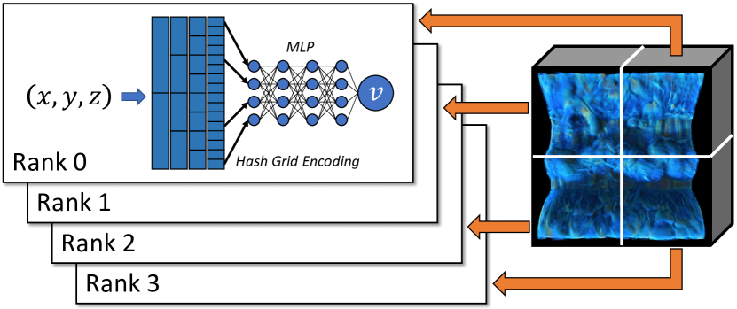
Figure 1: The architecture of our distributed neural representation.

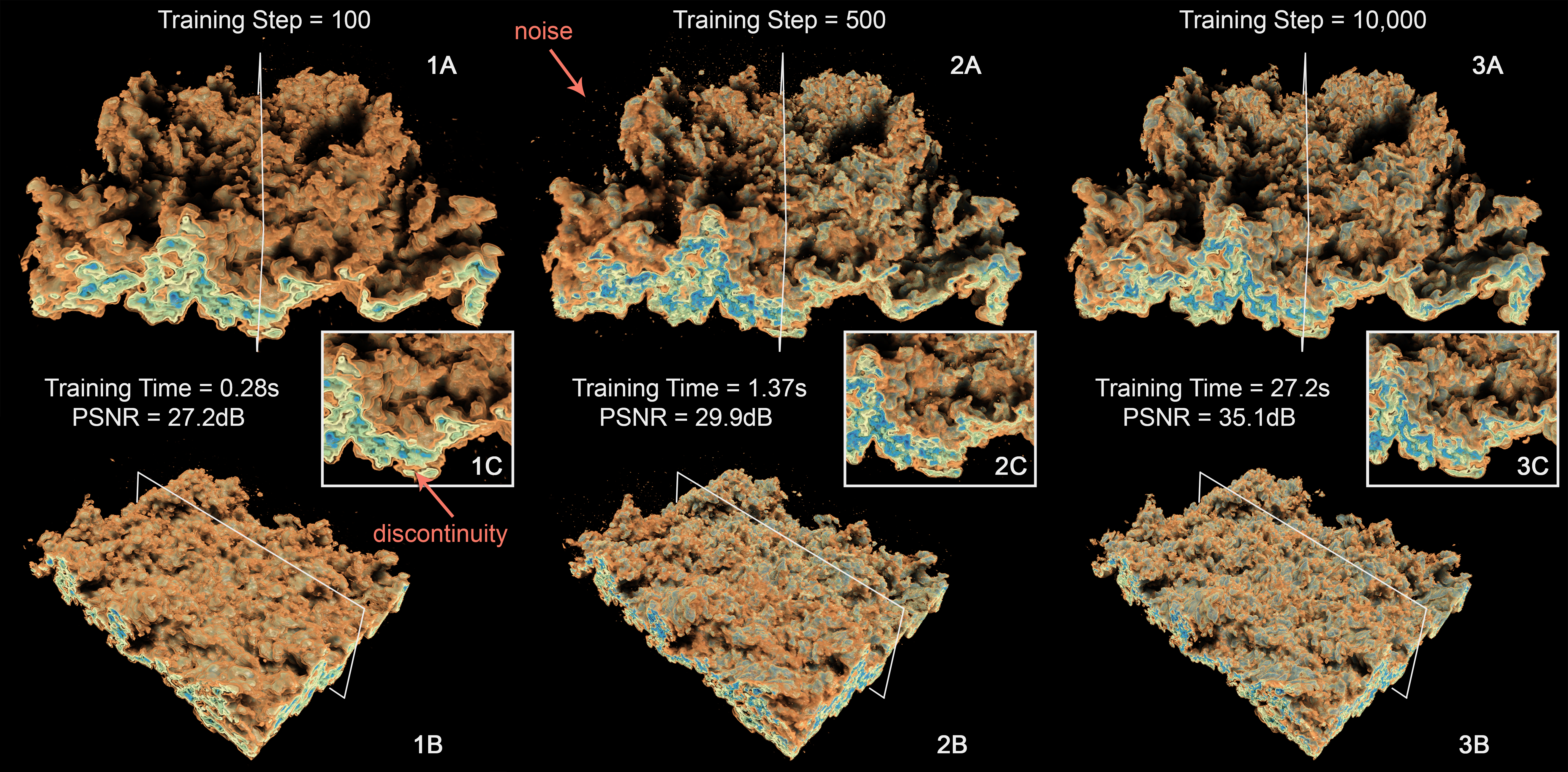
Figure 2: We compared the rendering of our distributed neural representations using varying numbers of training steps. The data was distributed to two MPI ranks and trained using two NVIDIA A100-40G GPUs on the ALCF Polaris supercomputer. Partition boundaries were highlighted using white lines in A) and B). C) are zoomed views of A) near partition boundaries. In 1C), an obvious discontinuity is visible at the partition boundary. With more training steps in 2), the discontinuity becomes less obvious, but high frequency noises are still visible. However, in 3), with sufficient training steps, these artifacts are no longer visible. We used flow field data generated from the S3D simulation [RGWC21] for this experiment.

3 Distributed Neural Representation (DNR)

Implicit neural representation (INR) is a neural network that is capable of directly approximating a volume field. It takes a spatial coordinate $(x,y,z)$ as input and outputs a value v corresponding to the volume field value at that coordinate, as represented by the equation:

$$\Phi:\mathbb{R}^{3}\rightarrow\mathbb{R}^{D},~{}(x,y,z)\mapsto\Phi(x,y,z)=\textbf{v}.$$ (1)

Here, v can be a scalar ($D=1$), 3-dimensional vector ($D=3$), or high-dimensional vector ($D>3$), depending on the specific problem. Our base INR architecture comprises a multi-resolution hash encoding layer [MESK22] and a small multilayer perceptron (MLP) network. The Rectified Linear Unit (ReLU) activation function is used in the hidden layers of the MLP.

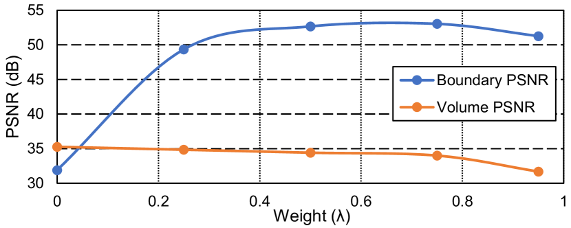
Figure 3: This plot depicts the impact of the weighting factor $\lambda$ on boundary connectivity and overall reconstruction quality. The blue curve represents the average image PSNR of two boundary slices relative to the ground truth slice, while the orange curve illustrates the average volume PSNR of two partitions relative to the ground truth volume. This plot is created using the S3D flow field data.

The neural network is trained by sampling input coordinates uniformly within the volume bounding box and computing the corresponding target values through appropriate interpolation methods utilizing reference data. To enhance network stability and accuracy, normalization of both input coordinates and output values to the range $[0,1]$ is performed.

During inference, the neural network can output v on-demand for any arbitrary coordinate within the volume domain, with low memory footprint and low computational cost. In certain cases, it may be necessary to decode the neural representation back to its original grid-based representation, making the technique compatible with existing visualization and analysis toolkits.

In the subsequent sections, we will demonstrate how this technique is adapted for use in distributed scenarios.

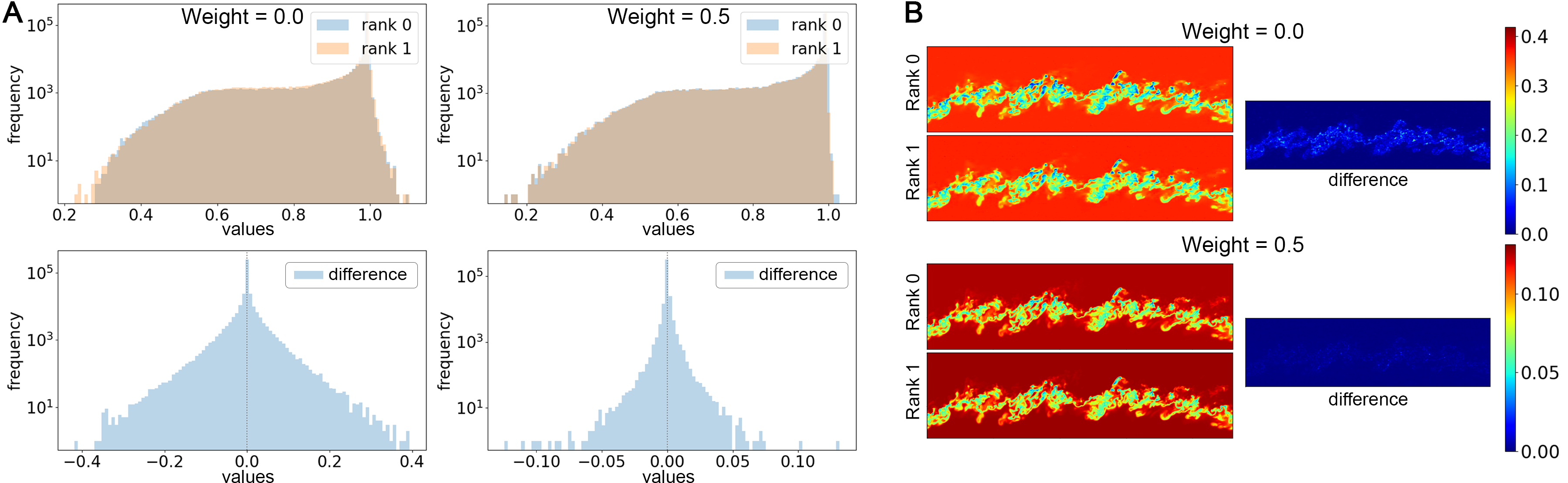
Figure 4: This figure compares the boundary slices of two neighboring partitions with two weighting factors, $\lambda$. A) displays histograms of the pixel values and their differences between the slices. B) shows pseudo-color plots of both slices and their differences. Both neural representations are trained for 10,000 steps. The S3D flow field data was used in this experiment.

3.1 Design of Distributed Neural Representation

We have devised a decentralized methodology for constructing INRs for distributed volume data. Our methodology involves creating a standard INR network on each MPI rank and training it using local data partitions. This results in the generation of numerous networks distributed across multiple ranks. To perform data analysis and visualization, we leverage standard parallel computing techniques. Our approach significantly reduces the need for data communication between ranks during the network training process, thus leading to a reduction in latency and improved performance. An overview of our technique is provided in Figure 1. In Figure 2, we highlight volume rendering results of neural representations with different optimization levels.

To maintain the continuity of the neural representation across partition boundaries during training, two techniques are utilized. Firstly, ghost regions are integrated into the training process and all networks are optimized to a consistent level of accuracy, aligning with the requirements of most existing distributed visualization algorithms. This is expected to result in highly scalable behavior as the training process can be executed independently on each rank, without the need of data communication. Secondly, a weighted loss term that prioritizes the continuity of the neural representation at partition boundaries is incorporated. The loss function takes the form of:

$$L_{\text{Total}}=(1-\lambda)~{}L_{1}(X_{\text{Uniform}},Y_{\text{Uniform}})+\lambda~{}L_{1}(X_{\text{Bound}},Y_{\text{Bound}}),$$ (2)

where $X_{\text{Uniform}}$ and $Y_{\text{Uniform}}$ are the reference and predicted volume values obtained from uniformly sampling the data, and $X_{\text{Bound}}$ and $Y_{\text{Bound}}$ are the ground truth and predicted volume values at the partition boundaries. $\lambda$ is a weighting factor that controls the influence of the boundary term on the overall loss.

To maximize the use of the input range of each local neural network, a global coordinate is first converted into the relative coordinate of a data partition and then normalized to the range of $[0,1]^{3}$. To ensure consistent neural network optimizations, different data partitions are also normalized using the same maximum and minimum values.

In Figure 3 we perform a parameter search to study the effectiveness of the weighting factor $\lambda$. We found that the existence of the boundary connectivity loss can significantly increase the data accuracy across the partition boundary. However, as the weight increases, we see a diminishing effect and a negative impact on the overall reconstruction quality. We believe that the sweet spot for $\lambda$ is 0.5 and we use this value in this paper. In Figure 4 we show a more detailed comparison between $\lambda=0.5$ and $\lambda=0.0$ (i.e., no boundary connectivity loss).

3.2 Implementation

We implemented the training system in PyTorch [PGM^∗19] and leveraged GPUs to accelerate the training process. To further optimize the implementation, we utilized the PyTorch API of Tiny-CUDA-NN [Mül21] for the multi-resolution hash encoding and multi-layer perceptions.

Our system employs an 16-level hash-grid encoding layer with 4 features per level. Each level uses a hash table of $2^{19}$ entries and the base level resolution is 4 with a scaling factor of 2. The multi-layer perception consists of 4 hidden layers with 64 neurons each. As mentioned before, ReLU activation functions are applied to all hidden layers. The output layer does not use an activation function.

We also utilized the Adam optimizer to train the neural network, with hyperparameters $\beta_{1}=0.9$ and $\beta_{2}=0.999$, to optimize for stability and convergence. To combat overfitting and improve convergence, we employed a learning rate schedule that starts at 1e-2 and decays by a factor of $0.8$ every 500 steps. Additionally, we used the loss function with a weighting $\lambda=0.5$.

4 DIVA and Ascent Integration

In this work, we first integrate the distributed neural representation technique into the DIVA reactive programming system and employ it to cache large volume fields. Then, we incorporate DIVA into Ascent, facilitating reactive programming in real-world in situ applications. This section presents details about our implementations.

4.1 Neural Representation Integration in DIVA

Classical reactive programming implementation guarantees unrestricted access to the history of time-varying values, which poses a significant challenge as it may lead to impractical data storage for some applications [EH97]. In order to address this challenge, DIVA [WNI^∗20] mandates explicit specification of the maximum number of time-steps to cache when defining related variables. Exceptions will be thrown if the system is unable to cache all the required time-steps, thereby limiting the expressiveness of reactive programming when dealing with volume fields. To overcome this limitation, we have incorporated DNR for efficient data caching. In the subsequent section, we present our implementation approach, specifically focusing on the methodology of constructing and inferring neural representations.

4.1.1 Constructing Neural Representation

We have developed a specialized construct called the neural volume object in DIVA, which encapsulates volume fields. Creating a neural volume object initiates the training of a DNR in PyTorch, which continues until the user-defined accuracy criterion (such as a PSNR target) is reached. Once the training concludes, access to the original volume field is revoked, and the learned neural network parameters are cached in system RAM for efficient storage and retrieval.

Notably, the neural volume object is implemented as a pure global entity in DIVA, which means that it is referentially transparent. However, the instantiation of the object may necessitate data synchronization across multiple parallel ranks. This attribute enables DIVA to streamline the workflow by avoiding the construction of a DNR if it is not ultimately accessed by any trigger actions on any ranks. If a DNR is generated, DIVA automatically synchronizes the metadata and training process to ensure accuracy.

⬇

1// declare a list of neural representation

2auto lst = nList({ neuralrepr });

3

4// declare a temporal cache of neural representation

5auto win = nNode("neuralrepr::window",

6 "in", neuralrepr, "size", 40 // maximum cache size

7);

8

9// declare volume rendering

10auto action = nNode("neuralrepr::render",

11 "volumes", win, // accept either "lst" or "win"

12 "image_prefix", "output_%04d", // filename format

13 "camera/elevation", 20 // camera settings

14);

15

16// trigger the volume rendering action based on a

17// pre-defined condition

18nTrigger(action, condition);

Listing 1: The DIVA workflow for creating a temporal window and applying volume rendering to the window when triggered.

DIVA is implemented in C++. To facilitate seamless integration with PyTorch, we leverage the pybind11 library [JRM17] to create bindings between C++ and Python. Specifically, we maintain an embedded Python interpreter inside C++, which is initialized at the start of the simulation. Using the Python interpreter, we construct DNR models and execute DNR training scripts. It is worth noting that the Python-side models and scripts are unaware of distributed data parallelism. Instead, all synchronization and data communication operations are handled on the C++ side through DIVA. This approach allows us to leverage PyTorch’s powerful machine learning capabilities while still maintaining the efficiency and scalability of our DIVA codebase.

To prevent data duplication, we utilize zero-copy numpy array views for passing volume data to Python scripts. To optimize memory usage during training, we generate training data samples on-demand using a custom volume sampler that supports backends for scalar and vector fields, as well as all volume mesh types used in Ascent. For uniform and rectilinear meshes, we provide a native data sampler that generates samples directly on the GPUs. In the case of more complex unstructured meshes, we implement data sampling using VTKm [MSU^∗16], which currently necessitates multiple data transfers between the CPU and the GPU for each training step due to the absence of a direct GPU API. To solve this inefficiency, we offer the option of resampling unstructured meshes into a uniform mesh. The optimization of our VTKm-based data samplers is left as future work.

4.1.2 Accessing Neural Representation

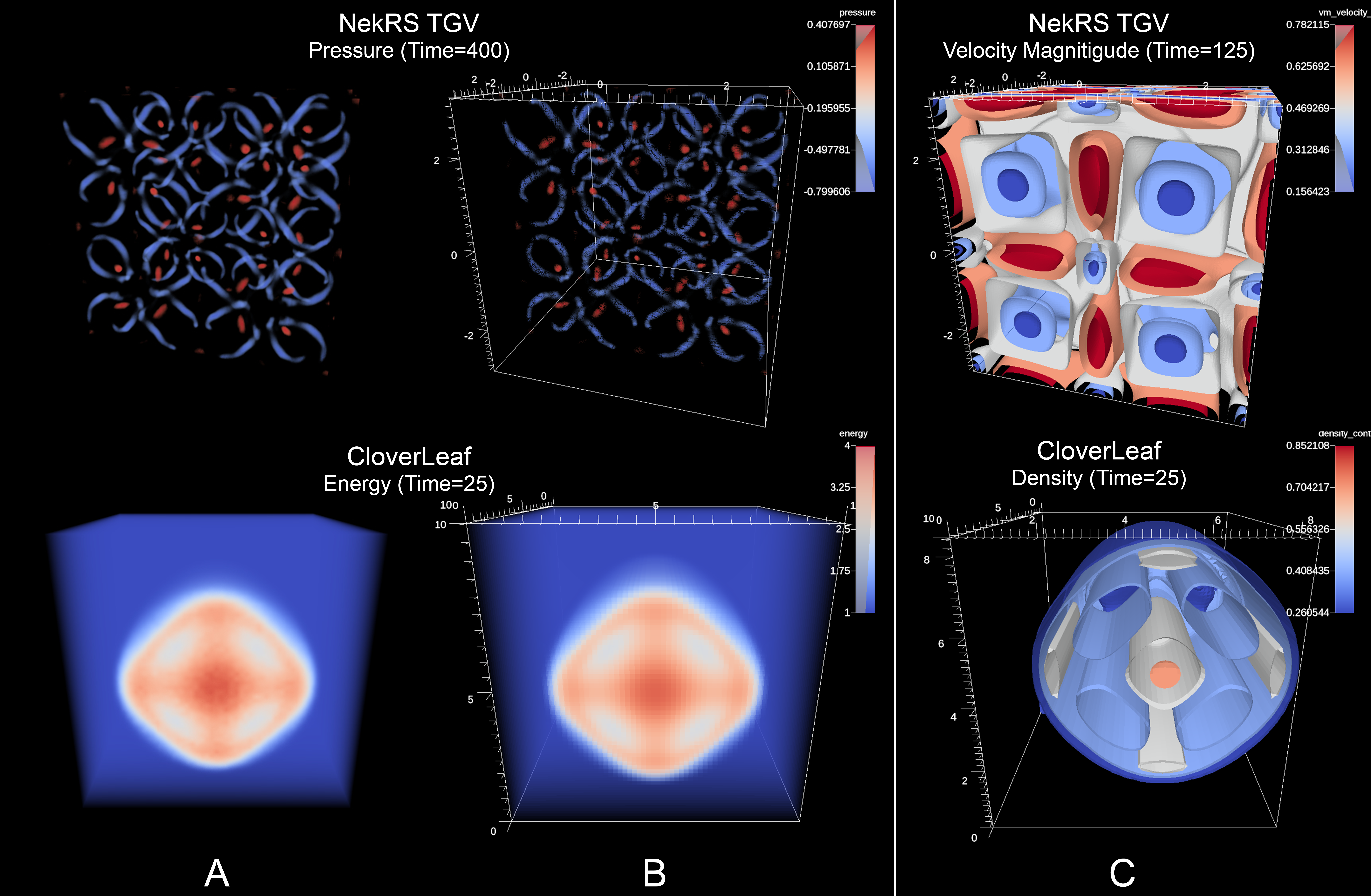
Figure 5: Visualization results generated by our DIVA-Ascent integration. A) Volume rendering of distributed neural representation generated using our neural rendering operator. B) Volume rendering of the ground truth data directly using the corresponding DIVA operator associated with Ascent’s renderer. C) Isosurfaces generated by the DIVA operator associated with Ascent’s contour filter.

To access the neural volume in subsequent sessions, we reconstruct the DNR network using PyTorch and calculate the required data values through inference. We provide two inference strategies in our implementation to ensure performance and compatibility. The neural network can be directly used as input for operations compatible with DNR, and the most appropriate inference method can be selected. For instance, our volume renderer utilizes the sample-streaming algorithm and the macro-cell acceleration structure proposed by Wu et al. [WBDM22] for optimization. Legacy operations like streamline tracers can decode the neural volume to a grid representation. We plan to offer DNR compatible routines for these operations in the future gradually.

4.1.3 Window Operator

DIVA enables access to variables’ histories through temporal pure operators. Among them, the window operator is one of the key operators. As shown in LABEL:fig:code-window, the window operator accepts an input variable and an integer size. It allows users to transform a time-varying variable into a temporal array. The constructed temporal array (i.e., win) can be used just like a normal array (e.g., lst) and can be used with any array operators for visualization and analysis. Users can also define trigger-like filters to exclude values from unwanted timesteps, but this feature is not demonstrated in this example for the sake of simplicity.

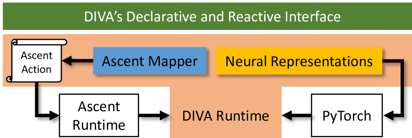
Figure 6: The overview of our DIVA-Ascent integration.

The implementation of the window operator uses DIVA’s internal temporal data caching mechanism to store the input variable’s values as the simulation progresses. As the number of cached values reaches the user-defined size, the earliest value gets removed to save space for new values. When applied to a volume field, the temporal data caching can quickly consume a lot of memory, causing scalability issues. Therefore, in this study, we have modified the window operator to support neural volumes. This modification enables users to create windows that are about 100$\times$ longer, thus overcoming the memory bottleneck.

4.1.4 Distributed Volume Rendering

Volume rendering is one of the most commonly used operations in visualization, thus an optimized routine to render our distributed neural representation is provided. Our neural network architecture is independent of volume mesh structures, and as a result, only one rendering algorithm is needed. We leverage previous work done by Wu et al. [WBDM22] and construct a base renderer using their sample-streaming algorithm. We aslo use their macro-cell acceleration structure for adaptive sampling. Then we add a sort-last parallel rendering system to support distributed neural representations. The renderer does not require decoding the neural representation back to a grid representation, consequently producing a very small memory footprint. However, as inferring an implicit neural network is inevitably more expensive than directly sampling a 3D GPU texture, our renderer produces a higher rendering latency.

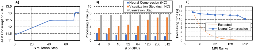
Figure 7: The direct volume rendering case running. A) The average peak RAM consumption of all the scaling runs with CloverLeaf3D. B) The weak scaling result with CloverLeaf3D. C) The strong scaling result with NekRS-TGV.

⬇

1// declare a set of isosurfaces

2auto contour = nNode("ascent::contour",

3 "field", density_field, "levels", 5

4);

5// declare a pseudocolor visualization

6auto plot = nNode("ascent::pseudocolor",

7 "field", contour

8);

9// declare a renderer to render the plot

10auto action = nNode("ascent::renderer",

11 "plots", nList({ plot }),

12 "image_prefix", "output_%04d",

13 "camera/elevation", 20.0

14);

15// trigger the volume rendering action based on a

16// pre-defined condition

17nTrigger(action, condition);

Listing 2: The DIVA workflow for creating a set of isosurfaces and applying Ascent’s renderer to visualize them when triggered.

4.2 DIVA Integration in Ascent

Ascent is a many-core capable flyweight in situ visualization and analysis infrastructure that many real-world multi-physics HPC simulations adopt [LAA^∗17]. To enable our method in real-world production environments directly, we also integrated DIVA into it. Figure 6 gives an overview of our implementation design. Major benefits include the ability to program event-driven in situ workflows using DIVA’s declarative interface and reactive programming abstractions. This not only reduces the complexity of writing an event-driven in situ workflow, but also improves the workflow performance as the DIVA runtime can perform lazy-evaluation and avoid needless re-computations.

The integration maps all the important Ascent concepts to DIVA. For example, it exposes fields as regular variables and enables them to be implicitly associated with a coordinate system and a topology. It also blurs the difference between filters, pipelines and expressions, and implements all of them as DIVA operators. Internally, the runtime can map different operators back to the corresponding Ascent concept, construct a valid volume mesh using zero-copy operations, and create an Ascent action to execute each individual operation. Using a customized zero-copy extractor, calculated results can be directly returned to the DIVA runtime and continue interacting with other components defined in the visualization workflow. The code snippet in LABEL:fig:code-contour illustrates how to use a contour filter with five uniform levels. LABEL:fig:code-contour-ascent illustrates how the same thing can be done in Ascent. Figure 5C displays the resulting images. As a result, this design choice makes DIVA more accessible.

⬇

1# Ascent contour filter with evenly spaced levels.

2-

3 action: "add_pipelines"

4 pipelines:

5 pl1:

6 f1:

7 type: "contour"

8 params:

9 field: "density"

10 levels: 5

11-

12 action: "add_scenes"

13 scenes:

14 s1:

15 plots:

16 p1:

17 type: "pseudocolor"

18 field: "density"

19 pipeline: "pl1"

20 renders:

21 r1:

22 camera:

23 elevation: 20.0

24 image_prefix: "output_%04d"

Listing 3: The Ascent action equivalent to LABEL:fig:code-contour.

Finally, our integration is very lightweight because it does not need additional adaptors in the simulation code. It can directly accept Conduit Blueprint mesh descriptions [HLR^∗22] and parse them to generate DIVA-specific data definitions. The only thing users have to do is call divaInitialize and divaFinalize at the beginning and end of the simulation, and then execute the DIVA workflow instead of Ascent actions in each visualization step. This makes it easy for any simulation that already uses Ascent to enable DIVA as an enhancing feature with minimal changes.

5 Case Studies

We conducted two case studies to effectively estimate the performance of our technique and implementation. Both cases were implemented in two production simulations, each with different mesh structures.

The first simulation, Cloverleaf3D, is a widely used open-source application for simulating multi-physics problems, particularly in computational fluid dynamics (CFD). It provided a straightforward and effective solution for simulating complex geometries and enabled researchers to explore various physical phenomena, such as combustion, turbulence, and heat transfer. The simulation employed a rectilinear mesh for simulation, and we designed the first case study to evaluate the performance and scalability of our technique for scalar field visualizations.

The second simulation, NekRS, is a high-performance, scalable, and parallel spectral element code for solving partial differential equations. It is being used in a broad range of scientific and engineering applications, including fluid mechanics, acoustics, and electromagnetics. The Taylor-Green Vortex (TGV) example is a specific benchmark utilized to evaluate NekRS’ performance and scalability. The Taylor-Green vortex is a well-known analytical solution for the Navier-Stokes equations that describe fluid flow, and NekRS employs an unstructured hexahedral mesh for the simulation. We designed the second case study to evaluate our technique’s effectiveness on flow field visualizations.

To ensure a robust evaluation of the performance of our technique and implementation, we benchmarked all cases on the Polaris supercomputer from the Argonne Leadership Computing Facility. Each Polaris compute node is equipped with 4 NVIDIA A100 GPUs and 1 AMD EPYC Milan CPU. We scaled all cases up to 128 compute nodes, each with 4 MPI ranks per node. Each MPI rank was bound to a single GPU following round-robin assignment. We evaluated our technique from multiple perspectives, including quality, correctness, and scalability.

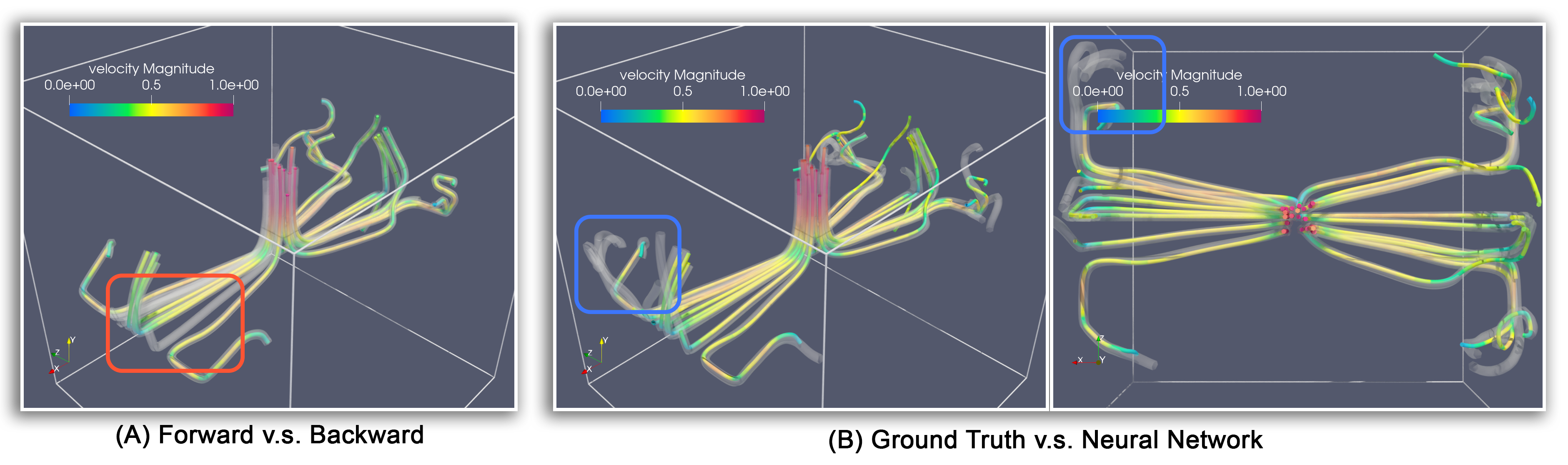
Figure 8: Pathline tracing results generated by our particle advection case. A) Comparing the backward (transparent tubes) and forward (solid tubes) pathline tracing of the same distributed neural representation. B) Comparing the backward tracing result of the ground truth data (transparent tubes) and distributed neural representation (solid tubes). Note that for B, the ground truth tracing was done post hoc. Our particle advection case directly outputs line data. All the renderings were generated using ParaView [AGL05].

5.1 Direct Volume Rendering

The first case study examined the utilization of direct volume rendering as a visualization technique for time-varying scalar fields. Specifically, an in situ approach was presented, which initiated the rendering process based on a pre-defined condition. The trigger condition was established as the first simulation step after time T, denoted by C=first(time>T). To generate a DNR of the volume field F, our neural volume operator was employed, which produced a representation R with a target peak signal-to-noise ratio (PSNR) Q, as denoted by R=encode(F,target_psnr=Q). Subsequently, a temporal array W of R was constructed, encompassing the N most recent simulation steps, by utilizing a window operator, expressed as W=window(R,size=N). Upon satisfying the trigger condition, the entire temporal array was rendered using a fixed visualization setting, as expressed by trigger(render(volumes=W,...),condition=C). It is noteworthy that the volume rendering algorithm employed here is described in Section 5.1.

The target reconstruction quality of $Q=45dB$ and a window size of $N=40$ were used. Volume rendering for CloverLeaf3D was initiated at approximately the $70^{th}$ timestep ($T=0.35s$), while for NekRS-TGV, it was triggered at the $500^{th}$ timestep ($T=5.75s$). At each step, we recorded the time spent on simulation computations, visualizations, and specifically the time spent on neural compression during the visualization period. In addition, we monitored the peak memory usage of each rank at each timestep by accessing the proc filesystem. Our results are presented in Figure 7. Given the limitations on space and the similarity of their behaviors, we only report the average peak RAM consumption of CloverLeaf3D runs (A), the weak scaling result of CloverLeaf3D (B), and the strong scaling result of NekRS-TGV (C).

The peak memory footprint generated by our implementation corresponded with our expectations. As shown in Figure 7A, a consistent rise in memory consumption was noticed during the initial 40 timesteps, which can be attributed to the caching of newly constructed neural representations. Post 40 steps, the memory consumption ceased to escalate since the temporal array generated by the window operator had reached its maximum capacity. As a result, the oldest neural representation was displaced to create room for new data. At the 70th timestep, an increase in memory consumption was observed, which was attributed to the allocation of memory by the volume rendering engine.

The case study also presented promising findings on weak scaling, as evidenced in Figure 7B. It was observed that the average time required to compute the neural compression decreased as the simulation scaled up. This outcome was attributed to the fact that, while the simulation resolution grew proportionally with the total number of MPI ranks, the physical event under investigation remained constant. As a result, the data complexity represented by each local grid declined, enabling the neural network to compress a grid with less “information” to the target PSNR using fewer training iterations. This outcome implies that the cost of running the neural compression algorithms correlates to the information complexity. Additionally, a slight increase in the overall visualization cost was observed, stemming from the MPI communications necessary for evaluating the DIVA workflow. It is worth noting that optimizing the DIVA workflow is beyond the scope of this study. As such, it is left as one of the future works.

We also evaluated the strong scaling behavior of the case study. Specifically, we conducted an experiment to assess the scaling of the neural compression time with respect to the number of MPI ranks. As shown in Figure 7C, we plotted the scaling behavior of the algorithm alongside the ideal strong scaling curve. Our findings revealed that the neural compression algorithm exhibited poor scaling behavior under these conditions. This result is not unexpected, given that even for a small domain, the neural network would still require multiple iterations to approximate the complex information presented in the volume field. In other words, the computational cost of compressing volume data using neural networks does not scale linearly with the data resolution.

5.2 Backward Particle Advection with VTKm

Pathline tracing is a well-established visualization technique for examining flow patterns in diverse fields, such as combustion, aerodynamics, and cosmology. Pathlines, which are integral curves of a time-varying vector field $V(\vec{x})$ beginning from a seed spatial coordinate $\vec{x_{0}}$ at time $t_{0}$, serve as the basis for this technique. Numerical integration algorithms, such as the Euler or Runge-Kutta methods, are frequently employed to compute pathlines. Pathlines can be integrated forward or backward in time, with the latter being particularly intriguing as it can aid in the identification of event-related regions and the comprehension of their causal relationships. However, backward integration poses significant challenges for in situ visualization, such as the impracticality of saving all generated data and the difficulty of establishing trigger conditions for time periods preceding a detectable event. Nevertheless, we demonstrate that our distributed neural representation makes backward integration a feasible task.

For the sake of simplicity and consistency, the same synthetic trigger condition as in the previous case study, C=first(time>T), was utilized. At the time when the trigger condition was activated, a set of $M$ seeds were randomly selected from a pre-defined bounding box. Subsequently, utilizing our encoding function, we produced a DNR $R$ of the velocity field $V$ with a target PSNR of $Q$. Following this, we constructed a long temporal window $W$ and applied array operators to reverse and negate the temporal window. Pathlines were then generated over this window, denoted as P=pathline(negate(reverse(W)),...). Upon triggering the condition, pathlines were computed and the resulting data was saved for further visualization and analysis.

VTKm was used to implement the pathline tracing operator even though it did not inherently support neural representations. To overcome this limitation, the velocity field was decoded back to the original mesh grid before being passed to the operator. This decoding process was performed on an on-demand basis, allowing for the retention of only two additional copies of the mesh grid at any given time. The operation of negate was executed in-place and multiplied all field values in all array entries by -1. Additionally, the reverse operation was applied, which simply entailed the alteration of the index of the $i$-th element to $N-i-1$.

We utilized the common settings inherited from the first case study to compute the forward and backward pathlines of both the neural representation and the ground truth data. It should be noted that the backward pathlines of the ground truth data were computed post hoc, requiring explicit caching of volume data to disk. This method proved to be inefficient, and as such, we were only able to achieve good scalability through the use of DNRs. The primary focus of this case study was to investigate the feasibility of utilizing DNR for pathline tracing, as well as analyzing the quality of the traced pathlines. To this end, we present two sets of comparisons in Figure 8.

We first compared the backward and forward tracing of a given velocity field (Figure 8A). Initially, we conducted a backward tracing process using a set of predetermined initial seeds. Subsequently, we identified the end point of all traced pathlines and utilized them as new seeds for the forward tracing process. Through this comparison, we aimed to verify the accuracy of our pathline tracing algorithm and validate the appropriateness of selected parameters for the tracing algorithm. Our findings revealed that the accuracy of backward tracing could be influenced by the integration step size. Nonetheless, provided that the step size remains reasonably small, both forward and backward tracing methods can yield nearly identical results. In Figure 8A, we depict the trajectories of particles traced backward in time using transparent tubes, while the forward pathlines are represented using solid tubes. The line color corresponds to the velocity of the particles. It is important to note that some solid forward pathlines are absent from the plot, as highlighted in the orange square. This does not signify inaccuracy in our approach; rather, it is due to the end points of some backward tracing pathlines falling outside the data domain. Consequently, these seeds were automatically ignored by the algorithm during the forward tracing pass.

Then, we employed backward tracing to examine both neural representations and ground truth fields. The resulting pathlines were subsequently compared, as illustrated in Figure 8B. Notably, the pathlines generated from neural representations were generally precise, with noticeable deviations from the ground truth observed only after many integration steps. Our analysis revealed that these deviations occurred primarily in regions where the velocity magnitudes were small. This finding is reasonable, as the neural compression noise in regions with small velocity magnitudes, could exert greater influence, thus leading to incorrect particle movements. Once such deviations occurred, it became impossible to rectify them.

6 Discussion and Future Work

We conducted a comprehensive evaluation of our technique from two distinct perspectives. Firstly, we investigated the correctness and quality of our distributed neural representation construction. Secondly, we focused on our distributed neural representation implementation in DIVA and our integration to the Ascent infrastructure by studying the usability and performance.

In terms of quality, our technique offers a simple yet effective approach to apply implicit neural representation to distributed data. We found that our method is able to achieve fairly high reconstruction quality in a matter of seconds due to the efficiency of the base neural network. By using ghost region information and introducing a weighted boundary loss, we were able to ensure boundary connectivity and reduce artifacts. Our case study results demonstrate that our neural representation has great potential and can be applied to a range of in situ visualization and analysis tasks. As it is capable of preserving many details presented in the data, it is suitable for many scientific visualization tasks such as volume rendering of scalar fields, as well as working with vector fields and integral lines, with reasonable accuracy. However, it should be used with care, as some of these tasks are more sensitive to errors.

In terms of usability, our distributed neural representation technique significantly reduces data size and can be used to achieve aggressive temporal data caching. This is essential for enabling the full potential of reactive programming for writing adaptive in situ workflows. Our integration in Ascent is easy to use, preserving most of its conventions and using the same simulation interface. We demonstrate that complicated tasks such as backward data analysis can now be easily achieved using DIVA.

In terms of performance, by taking advantage of well-established parallel rendering pipelines and the recently proposed INR rendering algorithm, our distributed neural representation technique can enable efficient and scalable visualization and analysis. The cost of neural compression remains constant as the simulation scales, making it particularly suitable for modern large-scale simulations. Our DIVA integration also scales well, as demonstrated in Figure 7. We only observe a slight increase in visualization costs due to communication overheads after scaling the application to many nodes.

7 Conclusion

In this paper, we propose a novel technique called distributed neural representation for constructing implicit neural representation for distributed data. We then present the implementation of this technique within the DIVA reactive programming system, which enables efficient temporal data caching. Finally, to enhance the applicability of our implementation, we integrate it into the Ascent infrastructure and showcase its ability to solve real-world problems. Our results indicate promising scalability and performance.

Our approach enables memory-efficient reactive programming, which takes an essential step towards realizing the full potential of reactive programming for adaptive in situ visualization and analysis. We anticipate that this work will inspire further research to advance the exascale evolution of data processing.

References

- [AGL05] Ahrens J., Geveci B., Law C.: ParaView: An End-User Tool for Large-Data Visualization. In Visualization Handbook. Butterworth-Heinemann, 2005, pp. 717–731.
- [BAB∗12] Bennett J. C., Abbasi H., Bremer P.-T., Grout R., Gyulassy A., Jin T., Klasky S., Kolla H., Parashar M., Pascucci V., Pebay P., Thompson D., Yu H., Zhang F., Chen J.: Combining In-Situ and in-Transit Processing to Enable Extreme-Scale Scientific Analysis. In Proc. Int. Conf. SC (2012), pp. 1–9.
- [CKR∗12] Chiw C., Kindlmann G., Reppy J., Samuels L., Seltzer N.: Diderot: a parallel DSL for image analysis and visualization. In Proc. 33rd ACM SIGPLAN Conf. PLDI (2012), pp. 111–120.
- [DB21] DeMarle D. E., Bauer A. C.: In situ visualization with temporal caching. Computing in Science & Engineering 23, 3 (2021), 25–33.
- [EH97] Elliott C., Hudak P.: Functional reactive animation. In Proc. 2nd ACM SIGPLAN ICFP (1997), p. 263–273. URL: https://doi.org/10.1145/258948.258973, doi:10.1145/258948.258973.
- [GYH∗20] Guo L., Ye S., Han J., Zheng H., Gao H., Chen D. Z., Wang J.-X., Wang C.: SSR-VFD: Spatial super-resolution for vector field data analysis and visualization. In Proceedings of IEEE Pacific Visualization Symposium (2020).
- [HLR∗22] Harrison C., Larsen M., Ryujin B. S., Kunen A., Capps A., Privitera J.: Conduit: A successful strategy for describing and sharing data in situ. In 2022 IEEE/ACM International Workshop on In Situ Infrastructures for Enabling Extreme-Scale Analysis and Visualization (ISAV) (2022), pp. 1–6. doi:10.1109/ISAV56555.2022.00006.
- [HW19] Han J., Wang C.: TSR-TVD: Temporal super-resolution for time-varying data analysis and visualization. IEEE transactions on visualization and computer graphics 26, 1 (2019), 205–215.
- [HW20] Han J., Wang C.: SSR-TVD: Spatial super-resolution for time-varying data analysis and visualization. IEEE Transactions on Visualization and Computer Graphics (2020).
- [HW22] Han J., Wang C.: Coordnet: Data generation and visualization generation for time-varying volumes via a coordinate-based neural network. IEEE Transactions on Visualization and Computer Graphics (2022).
- [HZCW21] Han J., Zheng H., Chen D. Z., Wang C.: STNet: An end-to-end generative framework for synthesizing spatiotemporal super-resolution volumes. IEEE Transactions on Visualization and Computer Graphics 28, 1 (2021), 270–280.
- [JGG∗17] Jain S., Griffin W., Godil A., Bullard J. W., Terrill J., Varshney A.: Compressed volume rendering using deep learning. In Proceedings of the Large Scale Data Analysis and Visualization (LDAV) Symposium. Phoenix, AZ (2017).
- [JRM17] Jakob W., Rhinelander J., Moldovan D.: pybind11 – seamless operability between c++11 and python, 2017. https://github.com/pybind/pybind11.
- [KLM22] Kim D., Lee M., Museth K.: Neuralvdb: High-resolution sparse volume representation using hierarchical neural networks. arXiv preprint arXiv:2208.04448 (2022).
- [LAA∗17] Larsen M., Ahrens J., Ayachit U., Brugger E., Childs H., Geveci B., Harrison C.: The ALPINE In Situ Infrastructure: Ascending from the Ashes of Strawman. In Proc. Workshop ISAV (2017), pp. 42–46.
- [LAC∗92] Lucas B., Abram G. D., Collins N. S., Epstein D. A., Gresh D. L., McAuliffe K. P.: An Architecture for a Scientific Visualization System. In Proc. 3rd Conf. VIS (1992), pp. 107–114.
- [LBCH22] Larsen M., Brugger E., Childs H., Harrison C.: Ascent: A flyweight in situ library for exascale simulations. In In Situ Visualization for Computational Science. Springer, 2022, pp. 255–279.
- [LHT∗21] Larsen M., Harrison C., Turton T. L., Sane S., Brink S., Childs H.: Trigger happy: Assessing the viability of trigger-based in situ analysis. In 2021 IEEE 11th Symposium on Large Data Analysis and Visualization (LDAV) (2021), IEEE, pp. 22–31.
- [LJLB21] Lu Y., Jiang K., Levine J. A., Berger M.: Compressive neural representations of volumetric scalar fields. In Computer Graphics Forum (2021), vol. 40, Wiley Online Library, pp. 135–146.
- [LWM∗18] Larsen M., Woods A., Marsaglia N., Biswas A., Dutta S., Harrison C., Childs H.: A flexible system for in situ triggers. In Proc. Workshop ISAV (2018), pp. 1–6.
- [MESK22] Müller T., Evans A., Schied C., Keller A.: Instant neural graphics primitives with a multiresolution hash encoding. ACM Transactions on Graphics (ToG) 41, 4 (2022), 1–15.
- [MIA∗07] McCormick P., Inman J., Ahrens J., Mohd-Yusof J., Roth G., Cummins S.: Scout: A Data-Parallel Programming Language for Graphics Processors. Parallel Comput. 33, 10 (2007), 648–662.
- [MLF∗16] Myers K., Lawrence E., Fugate M., Bowen C. M., Ticknor L., Woodring J., Wendelberger J., Ahrens J.: Partitioning a Large Simulation as It Runs. Technometrics 58, 3 (2016), 329–340.
- [MSU∗16] Moreland K., Sewell C., Usher W., Lo L.-T., Meredith J., Pugmire D., Kress J., Schroots H., Ma K.-L., Childs H., Larsen M., Chen C.-M., Maynard R., Geveci B.: VTK-m: Accelerating the Visualization Toolkit for Massively Threaded Architectures. IEEE Comput. Graph. Appl. 36, 3 (2016), 48–58.
- [Mül21] Müller T.: tiny-cuda-nn, 4 2021. URL: https://github.com/NVlabs/tiny-cuda-nn.
- [PGM∗19] Paszke A., Gross S., Massa F., Lerer A., Bradbury J., Chanan G., Killeen T., Lin Z., Gimelshein N., Antiga L., et al.: Pytorch: An imperative style, high-performance deep learning library. Advances in neural information processing systems 32 (2019).
- [RBGH14] Rautek P., Bruckner S., Gröller M. E., Hadwiger M.: ViSlang: A System for Interpreted Domain-Specific Languages for Scientific Visualization. IEEE Trans. Vis. Comput. Graph. 20, 12 (2014), 2388–2396.
- [RGWC21] Rieth M., Gruber A., Williams F. A., Chen J. H.: Enhanced burning rates in hydrogen-enriched turbulent premixed flames by diffusion of molecular and atomic hydrogen. Combustion and Flame (2021), 111740.
- [SBP∗15] Salloum M., Bennett J. C., Pinar A., Bhagatwala A., Chen J. H.: Enabling adaptive scientific workflows via trigger detection. In Proc. 1st Workshop ISAV (2015), pp. 41–45.
- [SLM04] Schroeder W. J., Lorensen B., Martin K.: The visualization toolkit: an object-oriented approach to 3D graphics. Kitware, 2004.
- [SMWH17] Satyanarayan A., Moritz D., Wongsuphasawat K., Heer J.: Vega-Lite: A Grammar of Interactive Graphics. IEEE Trans. Vis. Comput. Graph. 23, 1 (2017), 341–350.
- [SRHH16] Satyanarayan A., Russell R., Hoffswell J., Heer J.: Reactive Vega: A Streaming Dataflow Architecture for Declarative Interactive Visualization. IEEE Trans. Vis. Comput. Graph. 22, 1 (2016), 659–668.
- [SRM18] Shih M., Rozhon C., Ma K.-L.: A Declarative Grammar of Flexible Volume Visualization Pipelines. IEEE Trans. Vis. Comput. Graph. 25, 1 (2018), 1050–1059.
- [WBDM22] Wu Q., Bauer D., Doyle M. J., Ma K.-L.: Instant neural representation for interactive volume rendering. arXiv preprint arXiv:2207.11620 (2022).
- [WHW21] Weiss S., Hermüller P., Westermann R.: Fast neural representations for direct volume rendering. arXiv preprint arXiv:2112.01579 (2021).
- [WNI∗20] Wu Q., Neuroth T., Igouchkine O., Aditya K., Chen J. H., Ma K.-L.: Diva: A declarative and reactive language for in situ visualization. In 2020 IEEE 10th Symposium on Large Data Analysis and Visualization (LDAV) (2020), IEEE, pp. 1–11.
- [WSG∗21] Wurster S. W., Shen H.-W., Guo H., Peterka T., Raj M., Xu J.: Deep hierarchical super-resolution for scientific data reduction and visualization. arXiv preprint arXiv:2107.00462 (2021).
- [ZHW∗17] Zhou Z., Hou Y., Wang Q., Chen G., Lu J., Tao Y., Lin H.: Volume upscaling with convolutional neural networks. In Proceedings of the Computer Graphics International Conference (2017), pp. 1–6.