Generalized Fractional Negative Binomial Process

Abstract

In this paper, we introduce a generalized fractional negative binomial process (GFNBP) by time changing the fractional Poisson process with an independent Mittag-Leffler (ML) Lévy subordinator. We study its distributional properties and its connection to PDEs. We examine the long-range dependence (LRD) property of the GFNBP and show that it is not infinitely divisible. The space fractional and the non-homogeneous variants of the GFNBP are explored. Finally, simulated sample paths for the ML Lévy subordinator and the GFNBP are also presented.

1 Introduction

Counting processes and their connections to fractional differential equations have received considerable attention in recent years with wide applications in diverse disciplines of the applied sciences, namely, physics, image processing, infectious diseases modeling, hydrology, finance, and probability theory (see Timmermann and Nowak (1999), Laskin (2003), Kumar et al. (2020), Guler Dincer et al. (2022)). The fractional Poisson process (FPP) and the negative binomial (NB) process are the two most commonly used counting processes studied in literature. Laskin (2009) employed the FPPs in defining a new quantum coherent system and also studied fractional versions of the Bell polynomials, Bell numbers, and the Stirling numbers of the second kind. An application of the FPP in risk theory is discussed by Biard and Saussereau (2014). Some actuarial and clinical trial applications of NB process have been addressed in Grandell (1997) and Cook and Wei (2003).

In recent years, several fractional versions of the NB process have been developed using subordination techniques through stable and inverse stable subordinators (see Beghin and Macci (2014), Beghin (2015), and Vellaisamy and Maheshwari (2018)). These generalizations are time-fractional versions of the NB process. Apart from these, space-fractional versions of the NB process have also been studied in literature (see Orsingher and Polito (2012), Polito and Scalas (2016), Beghin and Vellaisamy (2018), and Maheshwari (2023)). For $0<\beta<1$, let $\{S_{\beta}(t)\}_{t\geq 0}$ be a $\beta$-stable subordinator with the Laplace transform $\mathbb{E}[e^{-uS_{\beta}(t)}]=e^{-tu^{\beta}}.$ The inverse $\beta$-stable subordinator $\{E_{\beta}(t)\}_{t\geq 0}$ is defined as

$$E_{\beta}(t)=\inf\{r\geq 0:S_{\beta}(r)>t\},\;t\geq 0.$$

Let $\mu>0$, $\rho>0$, and $\{\Gamma(t)\}_{t\geq 0}$ be a gamma process, where $\Gamma(t)\sim G(\mu,\rho t)$, which denotes the gamma distribution with scale parameter $\mu^{-1}$ and shape parameter $\rho t$. Then NB process can be considered as gamma subordinated variant of the Poisson process. Recently, Vellaisamy and Maheshwari (2018) presented a fractional NB process (FNBP) $\{\mathcal{Q}_{\beta}(t,\lambda)\}_{t\geq 0}$ using gamma subordination in FPP which is characterized as

$$\mathcal{Q}_{\beta}(t,\lambda)=N_{\beta}(\Gamma(t),\lambda),$$

where $\{N_{\beta}(t,\lambda)\}_{t\geq 0}$ is the FPP defined in Meerschaert et al. (2011). The Mittag-Leffler (ML) Lévy process is a well-known example of geometric stable process with non-decreasing paths. It may be used in place of the gamma subordinator to construct several time-changed stochastic processes that may exhibit additional properties due to Mittag-Leffler delay. In this paper, we present a generalized fractional negative binomial process (GFNBP) by time changing the FPP with an independent Mittag-Leffler (ML) Lévy subordinator. This process exhibits overdispersion and long-range dependence (LRD) properties. It is not infinitely divisible and may be useful in different areas.

The paper is structured as follows: In Section 2, we present some preliminary notations and definitions. In Section 3, we define the GFNBP and discuss its main characteristics along with LRD property. The underlying fractional PDEs are also obtained for the pmf of the GFNBP. We study the space-fractional and the non-homogeneous version of the GFNBP in Section 4. Finally, we present simulated sample paths for the ML Lévy subordinator and the GFNBP in Section 5.

2 Preliminaries

In this section, some notations and definitions are given which will be used in the subsequent sections. Let $\mathbb{R}$ and $\mathbb{C}$ denote the set of real and complex numbers, respectively. Let $\mathbb{Z}_{+}=\mathbb{N}\cup\{0\}$, where $\mathbb{N}$ is the set of natural numbers.

2.1 Special functions

Here, we present some special functions which are essential for development of results in this paper.
(i) Three parameters Mittag-Leffler function $L_{\beta,\gamma}^{\alpha}(z)$ is defined as (see Podlubny (1999), Prabhakar et al. (1971))

$$L_{\beta,\gamma}^{\alpha}(z)=\sum_{k=0}^{\infty}\frac{z^{k}}{k!\Gamma(\gamma+\beta k)}\frac{\Gamma(\alpha+k)}{\Gamma(\alpha)},\;\;\beta,\gamma,\alpha,z\in\mathbb{C}\text{ and }\text{Re}(\beta)>0,\text{Re}(\gamma)>0,\text{Re}(\alpha)>0.$$ (2.1)

(ii) For $z\in\mathbb{C}$ and $0<\alpha<1,$ the M-Wright function $M_{\alpha}(z)$ is defined by (see Gorenflo and Mainardi (2015))

$$M_{\alpha}(z)=\sum_{k=0}^{\infty}\frac{(-z)^{k}}{k!\Gamma(-\alpha n+(1-\alpha))}.$$

The generalized Wright function is defined by (Kilbas et al. (2002))

$$_{p}\psi_{q}\left[z\;\vline\;\begin{matrix}\left(\alpha_{i},\beta_{i}\right)_{1,p}\\ (a_{j},b_{j})_{1,q}\end{matrix}\right]=\sum_{k=0}^{\infty}\frac{z^{k}}{k!}\frac{\prod_{i=1}^{p}\Gamma(\alpha_{i}+\beta_{i}k)}{\prod_{j=1}^{q}\Gamma(a_{j}+b_{j}k)},\;\;z,\alpha_{i},a_{i}\in\mathbb{C}\;\text{and}\;\beta_{i},b_{i}\in\mathbb{R}.$$ (2.2)

(iii) A connection between the generalized Wright function and the H-function is (see Kilbas et al. (2002))

$$_{p}\psi_{q}\left[z\;\vline\;\begin{matrix}\left(\alpha_{i},\beta_{i}\right)_{1,p}\\ (a_{j},b_{j})_{1,q}\end{matrix}\right]=\;H_{p,q+1}^{1,p}\left[-z\;\vline\;\begin{matrix}\left(1-\alpha_{i},\beta_{i}\right)_{1,p}\\ (0,1)&(a_{j},b_{j})_{1,q}\end{matrix}\right],$$ (2.3)

where the H-function $H_{p,q+1}^{1,p}(z)$ can be expressed in terms of Mellin-Barnes type integral (see Kilbas et al. (2002)). For $k\in\mathbb{N},$ the $k$th order partial derivative of the H-function is given by (see Mathai et al. (2009))

$$\diffp{{}^{k}} \left[z^{-la_{1}/b_{1}}H_{p_{1},q_{1}}^{p_{2},q_{2}}\left[z^{l}\;\vline\;\begin{matrix}\left(\alpha_{i},\beta_{i}\right)_{1,p_{1}}\\ (a_{j},b_{j})_{1,q_{1}}\end{matrix}\right]\right]=z^{-k-(-la_{1}/b_{1})}\left(\frac{-l}{b_{1}}\right)^{k}H_{p_{1},q_{1}}^{p_{2},q_{2}}\left[z^{l}\;\vline\;\begin{matrix}\left(\alpha_{i},\beta_{i}\right)_{1,p_{1}}\\ (k+a_{1},b_{1}),&(a_{j},b_{j})_{2,q_{2}}\end{matrix}\right].$$ (2.4)

2.2 Definitions and some elementary distributions

(i) Let $f:[a,b]\subset\mathbb{R}\longrightarrow\mathbb{R}$ be such that $f(t)$ is $(n+1)$ times continuous differentiable for $n<\tau<n+1$. Then, the Riemann-Liouville fractional derivative of order $\tau>0$ is defined as (see Podlubny (1999))

$${}_{a}D^{\tau}_{t}f(t)=\bigg{(}\frac{d}{dt}\bigg{)}^{n+1}\int_{a}^{t}(t-u)^{n-\tau}f(u)du.$$

(ii) For $0<\beta\leq 1$, let $\{N_{\beta}(t,\lambda)\}_{t\geq 0}$ be a FPP with parameter $\lambda>0$. Its one- dimensional distributions are given by (see Laskin (2003), Meerschaert et al. (2011))

$$p_{\beta}(n/t,\lambda)=P[N_{\beta}(t,\lambda)=n]=\frac{(\lambda t^{\beta})^{n}}{n!}\sum_{k=0}^{\infty}\frac{(n+k)!}{k!}\frac{(-\lambda t^{\beta})^{k}}{\Gamma(\beta(k+n)+1)},\;\;n\in\mathbb{Z}_{+}.$$

(iii) Let $\Gamma(t)\sim G(\mu,\rho t)$. Its probability density function (pdf) is given by

$$f_{G}(x,t)=\frac{\mu^{\rho t}}{\Gamma(\rho t)}x^{\rho t-1}e^{-\mu x},\;\;x>0.$$

(iv) Barndorff-Nielsen (2000) and Kumar et al. (2019) discussed the Mittag-Leffler (ML) Lévy process with various properties. For $\alpha\in(0,1)$ and $\rho,\mu,t>0,$ let $\{M_{\alpha,\rho,\mu}(t)\}_{t\geq 0}$ be a ML Lévy process with Lévy measure density

$$\pi(x)=\frac{\alpha\rho}{x}L_{\alpha,1}^{1}\left(-\mu x^{\alpha}\right),\;\;x>0.$$ (2.5)

The Laplace transform of ML Lévy process is

$$\mathbb{E}\left(e^{-uM_{\alpha,\rho,\mu}(t)}\right)=\left(\frac{\mu}{\mu+u^{\alpha}}\right)^{\rho t}.$$ (2.6)

Using the conditioning argument, the pdf of ML Lévy process is obtained and is given as (see Kumar et al. (2019))

$$f_{M_{\alpha,\rho,\mu}(t)}(x)=\sum_{k=0}^{\infty}(-1)^{k}\frac{\mu^{\rho t+k}\Gamma(\rho t+k)}{\Gamma(\rho t)\Gamma(k+1)}\frac{x^{\alpha(\rho t+k)-1}}{\Gamma(\alpha(\rho t+k))},\;x>0,$$ (2.7)

The moments of $l$th order are of the following form

$$\mathbb{E}[M_{\alpha,\rho,\mu}^{l}(t)]=\frac{\rho t}{\mu^{l/\alpha}\Gamma(1-l)}B\left(1-\frac{l}{\alpha},\rho t+\frac{l}{\alpha}\right)\sim\frac{\Gamma(1-\frac{l}{\alpha})}{\mu^{l/\alpha}\Gamma(1-l)}(\rho t)^{l/\alpha},\;0<l<\alpha\;\text{as}\;t\rightarrow\infty,$$ (2.8)

where $B(z_{1},z_{2})=\frac{\Gamma(z_{1})\Gamma(z_{2})}{\Gamma(z_{1}+z_{2})},\text{Re}(z_{1})>0,\text{Re}(z_{2})>0$ represents the beta function.

3 Generalized Fractional Negative Binomial Process

Here, we define a generalized fractional negative binomial process $\{\mathcal{G}_{\alpha,\rho}^{\mu,\beta}(t,\lambda)\}_{t\geq 0}$ by replacing the gamma subordinator with an independent ML Lévy subordinator in the gamma subordinated form of the FNBP, that is,

$$\mathcal{G}_{\alpha,\rho}^{\mu,\beta}(t,\lambda):=N_{\beta}(M_{\alpha,\rho,\mu}(t),\lambda),\;\;t\geq 0.$$

The probability mass function (pmf) of $\{\mathcal{G}_{\alpha,\rho}^{\mu,\beta}(t,\lambda)\}_{t\geq 0}$, denoted by $p_{\alpha,\rho}^{\mu,\beta}(n,t)=P[\mathcal{G}_{\alpha,\rho}^{\mu,\beta}(t,\lambda)=n]$ is derived as

$$p_{\alpha,\rho}^{\mu,\beta}(n,t) =\int_{0}^{\infty}p_{\beta}(n/y,\lambda)f_{M_{\alpha,b,\mu}(t)}(y)dy$$

$$=\int_{0}^{\infty}\left(\frac{(\lambda y^{\beta})^{n}}{n!}\sum_{k=0}^{\infty}\frac{(n+k)!}{k!}\frac{(-\lambda y^{\beta})^{k}}{\Gamma(\beta(k+n)+1)}\right)f_{M_{\alpha,\rho,\mu}(t)}(y)dy$$

$$=\frac{\lambda^{n}}{n!}\sum_{k=0}^{\infty}\frac{(n+k)!}{k!}\frac{(-\lambda)^{k}}{\Gamma(\beta(k+n)+1)}\int_{0}^{\infty}y^{\beta(n+k)}f_{M_{\alpha,\rho,\mu}(t)}(y)dy$$

$$=\frac{\lambda^{n}}{n!}\sum_{k=0}^{\infty}\frac{(n+k)!}{k!}\frac{(-\lambda)^{k}}{\Gamma(\beta(k+n)+1)}\mathbb{E}M_{\alpha,\rho,\mu}^{\beta(k+n)}(t),\;\;0<\beta(k+n)<\alpha.$$

Remark 3.1.

For $\alpha=1$, the pmf of GFNBP reduces to

$$p_{1,\rho}^{\mu,\beta}(n,t)=\frac{\lambda^{n}}{n!}\sum_{k=0}^{\infty}\frac{(n+k)!}{\mu^{\beta(k+n)}k!}\frac{\Gamma((n+k)\beta+\rho t)(-\lambda)^{k}}{\Gamma(\rho t)\Gamma(\beta(k+n)+1)},$$

which is the pmf of the FNBP discussed in Vellaisamy and Maheshwari (2018).

Remark 3.2.

With the help of (2.8), the pmf $p_{\alpha,\rho}^{\mu,\beta}(n,t)$ can be expressed in terms of generalized Wright function of the following form

$$p_{\alpha,\rho}^{\mu,\beta}(n,t)=\frac{\lambda^{n}}{\mu^{\beta n/\alpha}n!\Gamma(\rho t)}\;_{3}\psi_{2}\left[\frac{-\lambda}{\mu^{\beta/\alpha}}\;\vline\;\begin{matrix}\left(n+1,1\right),&\left(1-\frac{\beta n}{\alpha},\frac{-\beta}{\alpha}\right),&\left(\rho t+\frac{\beta n}{\alpha},\frac{\beta}{\alpha}\right)\\ (1-\beta n,-\beta),&(1+\beta n,\beta)\end{matrix}\right].$$

Alternatively, it may be also expressed in terms of the $H$-function via the relation

$$p_{\alpha,\rho}^{\mu,\beta}(n,t)=\frac{\lambda^{n}}{\mu^{\beta n/\alpha}n!\Gamma(\rho t)}H_{2,3}^{1,2}\left[\frac{\lambda}{\mu^{\beta/\alpha}}\;\vline\;\begin{matrix}\left(-n,1\right),&\left(\frac{\beta n}{\alpha},\frac{-\beta}{\alpha}\right),&\left(1-\rho t-\frac{\beta n}{\alpha},\frac{\beta}{\alpha}\right)\\ (0,1),&(\beta n,-\beta),&(-\beta n,\beta)\end{matrix}\right].$$ (3.1)

Applying the Leibniz rule of derivative for the convolution of functions in (3.1) and with the help of (2.4), the partial differential equations (PDEs) governed by the pmf of GFNBP is

$$\diffp{{}^{k}}{\mu^{k}}p_{\alpha,\rho}^{\mu,\beta}(n,t)=\frac{1}{\mu^{\beta n/\alpha}n!\Gamma(bt)}\sum_{i=0}^{k}\binom{k}{i}\binom{n}{i}(-1)^{n-k}H_{2,3}^{1,2}\left[\frac{\lambda}{\mu^{\beta/\alpha}}\;\vline\;\begin{matrix}\left(-n,1\right),&\left(\frac{\beta n}{\alpha},\frac{-\beta}{\alpha}\right),&\left(1-\rho t-\frac{\beta n}{\alpha},\frac{\beta}{\alpha}\right)\\ (k-i,1),&(\beta n,-\beta),&(-\beta n,\beta)\end{matrix}\right],$$

with

$$p_{\alpha,\rho}^{\mu,\beta}(n,t)=\begin{cases}1&\text{if}\;\;n,t=0,\\ 0&\text{if}\;\;n\geq 1,\;t=0,\end{cases}\text{ and }p_{\alpha,\rho}^{\mu,\beta}(n,t)=0\text{ for all }\;n<0.$$

Next, we show that the pmf of the GFNBP satisfies a fractional PDE.

Lemma 3.1.

(Vellaisamy and Maheshwari (2018)) For $0<\tau\leq 1$, the governing fractional PDE for the gamma subordinator $\{\Gamma(t)\}_{t\geq 0}$ is given by

$$\diffp{{}^{\tau}}{t^{\tau}}f_{G}(x,t)=\rho\diffp{{}^{\tau-1}}{t^{\tau}}\left[\log\alpha+\log y-\psi(\rho t)\right]f_{G}(x,t),\;\;y>0\text{ and }f_{G}(x,0)=0,$$

where $\psi(x)$ is the digamma function and $\diffp{{}^{\tau}}{t^{\tau}}(\cdot)$ is the Riemann-Liouville fractional differential operator.

The next lemma gives the fractional version of PDE with respect to time variable satisfying the pdf of the ML Lévy process.

Lemma 3.2.

Let $g_{\alpha}(x,t)$ be the pdf for the $\alpha$-stable process. Then, the density of the ML Lévy process satisfies the following fractional PDE

$$\diffp{{}^{\tau}}{t^{\tau}}f_{M_{\alpha,\rho,\mu}(t)}(x)=\rho\diffp{{}^{\tau-1}}{t^{\tau-1}}\left[\left(\log\alpha-\psi(\rho t)\right)f_{M_{\alpha,\rho,\mu}(t)}(x)+\int_{0}^{\infty}g_{\alpha}(x,y)(\log y)f_{M_{\alpha,\rho,\mu}(t)}(y)dy\right].$$

Proof.

Consider

$$f_{M_{\alpha,\rho,\mu}(t)}(x)=\int_{0}^{\infty}g_{\alpha}(x,y)f_{G}(y,t)dy.$$

Operating the Riemann-Liouville fractional derivative, we get

$$\diffp{{}^{\tau}}{t^{\tau}}f_{M_{\alpha,\rho,\mu}(t)}(x) =\diffp{{}^{\tau}}{t^{\tau}}\int_{0}^{\infty}g_{\alpha}(x,y)f_{G}(y,t)dy$$

$$=\int_{0}^{\infty}g_{\alpha}(x,y)\diffp{{}^{\tau}}{t^{\tau}}f_{G}(y,t)dy$$

$$=\int_{0}^{\infty}g_{\alpha}(x,y)\left[\rho\diffp{{}^{\tau-1}}{t^{\tau}}\left[\log\alpha+\log y-\psi(\rho t)\right]f_{G}(y,t)\right]dy\;\;\;(\text{using Lemma \ref{lemm1}})$$

$$=\rho\diffp{{}^{\tau-1}}{t^{\tau-1}}\int_{0}^{\infty}g_{\alpha}(x,y)\left(\log\alpha-\psi(\rho t)\right)f_{G}(y,t)dy+\rho\int_{0}^{\infty}g_{\alpha}(x,y)(\log y)\diffp{{}^{\tau-1}}{t^{\tau-1}}f_{G}(y,t)dy.$$

With the help of simple algebra, the lemma follows. ∎

Now, using Lemma 3.2, we can get the governing fractional PDE for the GFNBP with respect to time variable of the form

$$\frac{1}{\rho}\diffp{{}^{\tau}}{t^{\tau}}p_{\alpha,\rho}^{\mu,\beta}(n,t)=\diffp{{}^{\tau-1}}{t^{\tau-1}}\left[\left(\log\alpha-\psi(\rho t)\right)p_{\alpha,\rho}^{\mu,\beta}(n,t)+\int_{0}^{\infty}\int_{0}^{\infty}p_{\beta}(n/s,\lambda)g_{\alpha}(x,y)(\log y)f_{M_{\alpha,\rho,\mu}(t)}(y)dyds\right],\;\text{with}\;p_{\alpha,\rho}^{\mu,\beta}(0,0)=1.$$

3.1 Mean, variance, autocovariance and index of dispersion

Theorem 3.1.

Let $\{\mathcal{G}_{\alpha,\rho}^{\mu,\beta}(t,\lambda)\}_{t\geq 0}$ be a GFNBP. For $0<s\leq t<\infty$, we have

(i) $\mathbb{E}[\mathcal{G}_{\alpha,\rho}^{\mu,\beta}(t,\lambda)]=q\mathbb{E}[M_{\alpha,\rho,\mu}^{\beta}(t)]\sim\frac{q\Gamma(1-\frac{\beta}{\alpha})}{\mu^{\beta/\alpha}\Gamma(1-\beta)}(\rho t)^{\beta/\alpha},\;0<\beta<\alpha.$ (ii) $\text{Var}[\mathcal{G}_{\alpha,\rho}^{\mu,\beta}(t,\lambda)]=q\mathbb{E}[M_{\alpha,\rho,\mu}^{\beta}(t)]-q^{2}\left(\mathbb{E}[M_{\alpha,\rho,\mu}^{\beta}(t)]\right)^{2}+2d\mathbb{E}[M_{\alpha,\rho,\mu}^{2\beta}(t)].$ (iii) Cov$[\mathcal{G}_{\alpha,\rho}^{\mu,\beta}(s,\lambda),\mathcal{G}_{\alpha,\rho}^{\mu,\beta}(t,\lambda)]=q\mathbb{E}[M_{\alpha,\rho,\mu}^{\beta}(t)]+d\mathbb{E}[M_{\alpha,\rho,\mu}^{2\beta}(s)]-q^{2}\mathbb{E}[M_{\alpha,\rho,\mu}^{\beta}(s)]\mathbb{E}[M_{\alpha,\rho,\mu}^{\beta}(t)]+q^{2}\beta\mathbb{E}\left[M_{\alpha,\rho,\mu}^{2\beta}(t)B\left(\beta,1+\beta;\frac{M_{\alpha,\rho,\mu}(s)}{M_{\alpha,\rho,\mu}(t)}\right)\right],$ where $q=\frac{\lambda}{\Gamma(1+\beta)},d=\beta q^{2}B(\beta,1+\beta),$ and $B(r,s;x)=\int_{0}^{x}t^{r-1}(1-t)^{s-1}dt$ for $0<x<1$ is an incomplete beta function.

Proof.

The mean, variance, and autocovariance functions of the FPP is given by (see Laskin (2003))

$$\mathbb{E}\left[N_{\beta}(t,\lambda)\right]=qt^{\beta},\;\;\;\;\text{Var}\left[N_{\beta}(t,\lambda)\right]=qt^{\beta}+Rt^{2\beta},$$ (3.2)

$$\text{Cov}\left[N_{\beta}(s,\lambda),N_{\beta}(t,\lambda)\right]=qs^{\beta}+ds^{2\beta}+q^{2}\left[\beta t^{2\beta}B(\beta,1+\beta;s/t)-(st)^{\beta}\right],\;\;0<s\leq t.$$

Using the conditioning argument and with the help of (3.2) and (2.8), Part (i) of the theorem can be easily obtained. Also, one may derive that

$$\mathbb{E}\left[N_{\beta}(s,\lambda)N_{\beta}(t,\lambda)\right]=qs^{\beta}+ds^{2\beta}+q^{2}\left[\beta t^{2\beta}B(\beta,1+\beta;s/t)\right],$$

that gives

$$\mathbb{E}\left[\mathcal{G}_{\alpha,\rho}^{\mu,\beta}(s,\lambda)\mathcal{G}_{\alpha,\rho}^{\mu,\beta}(t,\lambda)\right] =\mathbb{E}\left[\mathbb{E}\left[N_{\beta}(M_{\alpha,\rho,\mu}(s))N_{\beta}(M_{\alpha,\rho,\mu}(t))|(M_{\alpha,\rho,\mu}(s),M_{\alpha,\rho,\mu}(t))\right]\right]$$

$$=q\mathbb{E}[M_{\alpha,\rho,\mu}^{\beta}(t)]+d\mathbb{E}[M_{\alpha,\rho,\mu}^{2\beta}(s)]+q^{2}\beta\mathbb{E}\left[M_{\alpha,\rho,\mu}^{2\beta}(t)B\left(\beta,1+\beta;\frac{M_{\alpha,\rho,\mu}(s)}{M_{\alpha,\rho,\mu}(t)}\right)\right].$$

Now, the covariance formula gives Part (iii) of the theorem. Part (ii) is a consequence of Part (iii), when $s=t$. ∎

To study the index of dispersion of GFNBP, we first prove the following lemma.

Lemma 3.3.

For $0<l<\alpha/2,$ we have

$$\left(\mathbb{E}\left[M_{\alpha,b,\mu}^{l}(t)\right]\right)^{2}\leq\mathbb{E}\left[M_{\alpha,b,\mu}^{2l}(t)\right].$$

Proof.

By self-similar property of the stable processes, we get

$$\mathbb{E}[M_{\alpha,\rho,\mu}^{2l}(t)]=\mathbb{E}[G_{\mu,\rho}^{2l/\alpha}(t)]\mathbb{E}[S_{\alpha}^{2l}(1)]\geq\mathbb{E}[G_{\mu,\rho}^{l/\alpha}(t)]^{2}\mathbb{E}[S_{\alpha}^{l}(1)]^{2}=\left(\mathbb{E}[M_{\alpha,\rho,\mu}^{l}(t)]\right)^{2}.$$

∎

A stochastic process $\{X(t)\}_{t\geq 0}$ is overdispesed if $Var[X(t)]-\mathbb{E}[X(t)]>0$ for all $t\geq 0$ (see (Cox and Lewis, 1966, p. 72)). Using Lemma 3.3, we have

$$\text{Var}[\mathcal{G}_{\alpha,\rho}^{\mu,\beta}(t,\lambda)]-\mathbb{E}[\mathcal{G}_{\alpha,\rho}^{\mu,\beta}(t,\lambda)] =2d\mathbb{E}[M_{\alpha,\rho,\mu}^{2\beta}(t)]-\left(q\mathbb{E}[M_{\alpha,\rho,\mu}^{\beta}(t)]\right)^{2}=\frac{\lambda^{2}}{\beta}\left(\frac{\mathbb{E}\left[M_{\alpha,\rho,\mu}^{2\beta}(t)\right]}{\Gamma(2\beta)}-\frac{\left(\mathbb{E}\left[M_{\alpha,\rho,\mu}^{\beta}(t)\right]\right)^{2}}{\beta\Gamma^{2}(\beta)}\right)\geq 0.$$

It is clear from the fact that $\frac{\lambda^{2}}{\beta}\left(\frac{1}{\Gamma(2\beta)}-\frac{1}{\beta\Gamma^{2}(\beta)}\right)>0$ for $\lambda>0$ and $\beta\in(0,1)$ (see Beghin and Macci (2014)). Therefore, GFNBP exhibits overdispersion.

3.2 Laplace transform

Let $q(x,t)$ be the pdf of the $E_{\beta}\left(M_{\alpha,\rho,\mu}(t)\right)$ and $h_{\beta}(x,t)$ be the pdf of the inverse stable subordinator $E_{\beta}(t)$ with Laplace transform $\mathbb{E}[e^{-uE_{\beta}(t)}]=L_{\beta,1}^{1}(-ut^{\beta})$ (see Meerschaert and Straka (2013)). Then, the Laplace transform of $E_{\beta}\left(M_{\alpha,\rho,\mu}(t)\right)$ can be derived as

$$\mathbb{E}\left[e^{-uE_{\beta}\left(M_{\alpha,\rho,\mu}(t)\right)}\right] =\int_{0}^{\infty}e^{-ux}q(x,t)=\int_{0}^{\infty}\int_{0}^{\infty}e^{-ux}h_{\beta}(x,y)f_{M_{\alpha,\rho,\mu}(t)}(y)dydx$$

$$=\int_{0}^{\infty}L_{\beta,1}^{1}(-uy^{\beta})f_{M_{\alpha,\rho,\mu}(t)}(y)dy$$

$$=\sum_{k=0}^{\infty}\frac{(-u)^{k}}{\Gamma(1+\beta k)}\mathbb{E}[M_{\alpha,\rho,\mu}^{k\beta}(t)]\;\;(0<\beta k<\alpha)$$

$$=\frac{1}{\Gamma(\rho t)}\;_{2}\psi_{2}\left[\frac{-u}{\mu^{\beta/\alpha}}\;\vline\;\begin{matrix}\left(1,-\frac{\beta}{\alpha}\right),&\left(\rho t,\frac{\beta}{\alpha}\right)\\ (1,\beta),&(1,-\beta)\end{matrix}\right].$$

Using the conditioning arguments, we obtain the Laplace transform for the GFNBP as

$$\mathbb{E}\left[e^{-u\mathcal{G}_{\alpha,\rho}^{\mu,\beta}(t)}\right] =\mathbb{E}\left[\mathbb{E}\left[\text{exp}\left(-\lambda E_{\beta}\left(M_{\alpha,\rho,\mu}(t)\right)(1-e^{-u})\right)/E_{\beta}\left(M_{\alpha,\rho,\mu}(t)\right)\right]\right]$$

$$=\frac{1}{\Gamma(\rho t)}\;_{2}\psi_{2}\left[\frac{-\lambda(1-e^{-u})}{\mu^{\beta/\alpha}}\;\vline\;\begin{matrix}\left(1,-\frac{\beta}{\alpha}\right),&\left(\rho t,\frac{\beta}{\alpha}\right)\\ (1,\beta),&(1,-\beta)\end{matrix}\right].$$

Remark 3.3.

The probability generating function of the GFNBP can be deduced from the Laplace transform and is given by

$$\mathbb{E}\left[u^{\mathcal{G}_{\alpha,\rho}^{\mu,\beta}(t)}\right]=\frac{1}{\Gamma(\rho t)}\;_{2}\psi_{2}\left[\frac{-\lambda(1-u)}{\mu^{\beta/\alpha}}\;\vline\;\begin{matrix}\left(1,\frac{-\beta}{\alpha}\right),&\left(\rho t,\frac{\beta}{\alpha}\right)\\ (1,\beta),&(1,-\beta)\end{matrix}\right].$$

3.3 Infinite divisibility

The following self-similarity properties of stable and inverse stable subordinators will be used (see Meerschaert and Scheffler (2004))

$$S_{\alpha}(t)\stackrel{{\scriptstyle d}}{{=}}t^{1/\alpha}S_{\alpha}(1)\text{ and }E_{\beta}(t)\stackrel{{\scriptstyle d}}{{=}}t^{\beta}E_{\beta}(1),$$ (3.3)

where $\stackrel{{\scriptstyle d}}{{=}}$ stands for equality in distribution. Also, we may observe that

$$N_{\beta}(t,\lambda)\stackrel{{\scriptstyle d}}{{=}}N\left(E_{\beta}(t),\lambda\right)\stackrel{{\scriptstyle d}}{{=}}N\left(t^{\beta}E_{\beta}(1),\lambda\right).$$

By the renewal theorem (see Vellaisamy and Maheshwari (2018)), we get

$$\lim_{t\rightarrow\infty}\frac{N\left(t^{\beta}E_{\beta}(1),\lambda\right)}{t^{\beta}}=\lambda E_{\beta}(1)\;a.s.$$

Theorem 3.2.

The GFNBP $\{\mathcal{G}_{\alpha,\rho}^{\mu,\beta}(t,\lambda)\}_{t\geq 0}$ is not infinitely divisible.

Proof.

Using (3.3), we get

$$\mathcal{G}_{\alpha,\rho}^{\mu,\beta}(t,\lambda) =N_{\beta}(M_{\alpha,\rho,\mu}(t),\lambda)=N_{\beta}(S_{\alpha}(G_{\mu,\rho}(t)),\lambda)=N\left(\left[S_{\alpha}G_{\mu,\rho}(t)\right]^{\beta}E_{\beta}(1),\lambda\right)$$

$$=N\left(\left\{\left[G_{\mu,\rho}(t)\right]^{1/\alpha}S_{\alpha}(1)\right\}^{\beta}E_{\beta}(1),\lambda\right)=N\left(\left[G_{\mu,\rho}(t)\right]^{\beta/\alpha}\left(S_{\alpha}(1)\right)^{\beta}E_{\beta}(1),\lambda\right).$$

Now, we consider

$$\lim_{t\rightarrow\infty}\frac{N\left(\left[G_{\mu,\rho}(t)\right]^{\beta/\alpha}\left(S_{\alpha}(1)\right)^{\beta}E_{\beta}(1),\lambda\right)}{t^{\beta/\alpha}}$$

$$\stackrel{{\scriptstyle d}}{{=}}\lim_{t\rightarrow\infty}\frac{N\left(\left[G_{\mu,\rho}(t)\right]^{\beta/\alpha}\left(S_{\alpha}(1)\right)^{\beta}E_{\beta}(1),\lambda\right)}{\left[G_{\mu,\rho}(t)\right]^{\beta/\alpha}\left(S_{\alpha}(1)\right)^{\beta}E_{\beta}(1)}\frac{\left[G_{\mu,\rho}(t)\right]^{\beta/\alpha}\left(S_{\alpha}(1)\right)^{\beta}E_{\beta}(1)}{t^{\beta/\alpha}}$$

$$\stackrel{{\scriptstyle d}}{{=}}\;\;\;\lambda E_{\beta}(1)\left(S_{\alpha}(1)\right)^{\beta}\lim_{t\rightarrow\infty}\left(\frac{G_{\mu,\rho}(t)}{t}\right)^{\beta/\alpha}$$

$$\stackrel{{\scriptstyle d}}{{=}}\;\;\;\lambda E_{\beta}(1)\left(S_{\alpha}(1)\right)^{\beta}\left(\mathbb{E}G_{\mu,\rho}(1)\right)^{\beta/\alpha}.$$

For a large t, $G_{\mu,\rho}(t)/{t}\rightarrow\mathbb{E}G_{\mu,\rho}(1).$ Since $E_{\beta}(1)$ is not infinitely divisible, the result follows. ∎

3.4 Dependence structure

Definition 3.1.

For $0<s<t,$ let the correlation function Corr$[X(s),X(t)]$ for a stochastic process $\{X(t)\}_{t\geq 0}$ satisfies the following relation

$$c_{1}(s)t^{-d}\leq\text{ Corr}[X(s),X(t)]\leq c_{2}(s)t^{-d}$$

for large $t$, $d>0$, $c_{1}(s)>0$ and $c_{2}(s)>0.$ Expressly

$$\lim_{t\rightarrow\infty}\frac{\text{ Corr}[X(s),X(t)]}{t^{-d}}=c(s),$$

for some $c(s)>0$ and $d>0$. The process $\{X(t)\}_{t\geq 0}$ is said to have the LRD property if $d\in(0,1)$.

The following lemma can be proved exactly in a similar fashion as Lemma 2 in Maheshwari and Vellaisamy (2016).

Lemma 3.4.

Let $\beta\in(0,\alpha)$ and $0<s<t,s$ is fixed. Then, the following asymptotic expansion holds for a large t.

$$\text{(i)}\;\;\mathbb{E}\left[M_{\alpha,\rho,\mu}^{\beta}(s)M_{\alpha,\rho,\mu}^{\beta}(t)\right]\sim\mathbb{E}\left[M_{\alpha,\rho,\mu}^{\beta}(s)\right]\mathbb{E}\left[M_{\alpha,\rho,\mu}^{\beta}(t-s)\right].$$

$$\text{(ii)}\;\;\beta\mathbb{E}\left[M_{\alpha,\rho,\mu}^{2\beta}(t)B\left(\beta,1+\beta;\frac{M_{\alpha,\rho,\mu}(s)}{M_{\alpha,\rho,\mu}(t)}\right)\right]\sim\mathbb{E}\left[M_{\alpha,\rho,\mu}^{\beta}(s)\right]\mathbb{E}\left[M_{\alpha,\rho,\mu}^{\beta}(t-s)\right].$$

Theorem 3.3.

The GFNBP exhibits the LRD property.

Proof.

Using (2.8) and with the help of Lemma 3.4(ii), the asymptotic behaviour of Theorem 3.1(iii) is

$$\text{Cov}[\mathcal{G}_{\alpha,\rho}^{\mu,\beta}(s,\lambda),\mathcal{G}_{\alpha,\rho}^{\mu,\beta}(t,\lambda)] \sim q\mathbb{E}[M_{\alpha,\rho,\mu}^{\beta}(t)]+d\mathbb{E}[M_{\alpha,\rho,\mu}^{2\beta}(s)]-q^{2}\mathbb{E}[M_{\alpha,\rho,\mu}^{\beta}(s)]\left[\mathbb{E}[M_{\alpha,\rho,\mu}^{\beta}(t)]-\mathbb{E}\left[M_{\alpha,\rho,\mu}^{\beta}(t-s)\right]\right]$$

$$\sim q\mathbb{E}[M_{\alpha,\rho,\mu}^{\beta}(t)]+d\mathbb{E}[M_{\alpha,\rho,\mu}^{2\beta}(s)]-q^{2}\mathbb{E}[M_{\alpha,\rho,\mu}^{\beta}(s)]\left[\frac{\Gamma(1-\frac{\beta}{\alpha})}{\mu^{\beta/\alpha}\Gamma(1-\beta)}(\rho t)^{\beta/\alpha}-\frac{\Gamma(1-\frac{\beta}{\alpha})}{\mu^{\beta/\alpha}\Gamma(1-\beta)}(\rho(t-s))^{\beta/\alpha}\right]$$

$$\sim q\mathbb{E}[M_{\alpha,\rho,\mu}^{\beta}(t)]+d\mathbb{E}[M_{\alpha,\rho,\mu}^{2\beta}(s)].\;\;\;(\text{since}\;\;t^{\beta/\alpha}-(t-s)^{\beta/\alpha}\sim\beta\alpha^{-1}st^{(\beta/\alpha)-1})$$

Also, the asymptotic behaviour of Theorem 3.1(ii) follows

$$\text{Var}\left[\mathcal{G}_{\alpha,\rho}^{\mu,\beta}(t,\lambda)\right] \sim\left(\frac{\rho t}{\mu}\right)^{2\beta/\alpha}\left(\frac{2d\Gamma(1-\frac{2\beta}{\alpha})}{\Gamma(1-2\beta)}-\left(\frac{q\Gamma(1-\frac{\beta}{\alpha})}{\Gamma(1-\beta)}\right)^{2}\right)\sim t^{2\beta/\alpha}d_{1},$$

where $d_{1}=\left(\frac{\rho}{\mu}\right)^{2\beta/\alpha}\left(\frac{2d\Gamma(1-\frac{2\beta}{\alpha})}{\Gamma(1-2\beta)}-\left(\frac{q\Gamma(1-\frac{\beta}{\alpha})}{\Gamma(1-\beta)}\right)^{2}\right)$. Therefore, we have the correlation function as

$$\text{Corr}\left[\mathcal{G}_{\alpha,\rho}^{\mu,\beta}(s),\mathcal{G}_{\alpha,\rho}^{\mu,\beta}(t)\right] =\frac{\text{Cov}\left[\mathcal{G}_{\alpha,\rho}^{\mu,\beta}(s),\mathcal{G}_{\alpha,\rho}^{\mu,\beta}(t)\right]}{\sqrt{\text{Var}\left[\mathcal{G}_{\alpha,\rho}^{\mu,\beta}(s)\right]}\sqrt{\text{Var}\left[\mathcal{G}_{\alpha,\rho}^{\mu,\beta}(t)\right]}}\sim t^{-\beta/\alpha}\left(\frac{q\mathbb{E}[M_{\alpha,\rho,\mu}^{\beta}(s)]+d\mathbb{E}[M_{\alpha,\rho,\mu}^{2\beta}(s)]}{\sqrt{d_{1}\text{Var}\left[\mathcal{G}_{\alpha,\rho}^{\mu,\beta}(s)\right]}}\right).$$

Hence, for $0<\beta<\alpha$ and the decaying power $t^{-\beta/\alpha}$, the GFNBP has the LRD property. ∎

4 Space Fractional and Non-Homogeneous Versions

4.1 Space fractional version of the GFNBP

Orsingher and Polito (2012) have studied the space fractional Poisson process (SFPP) which is characterized as the Poisson process time-changed by independent stable subordinator. Let $\{N_{\alpha^{\prime}}(t,\lambda)\}_{t\geq 0},\;0<\alpha^{\prime}<1$ be a SFPP with pmf

$$p_{\alpha^{\prime}}(n/t,\lambda)=\frac{(-1)^{n}}{n!}\sum_{k=0}^{\infty}\frac{(-\lambda^{\alpha^{\prime}}t)^{k}}{k!}\frac{\Gamma(k{\alpha^{\prime}}+1)}{\Gamma(k{\alpha^{\prime}}+1-n)},\;\lambda>0.$$ (4.1)

Here, we present a space fractional version of the GFNBP by subordinating the SFPP with an independent ML Lévy subordinator. We denote it by $\{\mathcal{H}_{\alpha,\rho}^{\mu,\alpha^{\prime}}(t,\lambda)\}_{t\geq 0}$ and is defined as

$$\mathcal{H}_{\alpha,\rho}^{\mu,\alpha^{\prime}}(t,\lambda)=N_{\alpha^{\prime}}(M_{\alpha,\rho,\mu}(t),\lambda),\;\;t\geq 0.$$

Using (2.5) and the formula given in p. 197 of Ken-Iti (1999), one may calculate the Lévy measure density $\mathcal{V}$ for the process $\{\mathcal{H}_{\alpha,\rho}^{\mu,\alpha^{\prime}}(t,\lambda)\}_{t\geq 0}$ as

$$\mathcal{V}(k) =\int_{0}^{\infty}\sum_{i=1}^{\infty}p_{\alpha^{\prime}}(i/t,\lambda)\delta_{\{i\}}(k)\pi(t)dt$$

$$=\int_{0}^{\infty}\sum_{i=1}^{\infty}\left(\frac{(-1)^{i}}{i!}\sum_{j=0}^{\infty}\frac{(-\lambda^{\alpha^{\prime}}t)^{j}}{j!}\frac{\Gamma(j{\alpha^{\prime}}+1)}{\Gamma(j{\alpha^{\prime}}+1-i)}\right)\delta_{\{i\}}(k)\pi(t)dt$$

$$=\rho\sum_{i=1}^{\infty}\frac{(-1)^{i}}{i!}\delta_{\{i\}}(k)\sum_{j=0}^{\infty}\frac{(-\lambda^{\alpha^{\prime}})^{j}}{j!}\frac{\Gamma(j{\alpha^{\prime}}+1)}{\Gamma(j{\alpha^{\prime}}+1-i)}\int_{0}^{\infty}\alpha t^{j-1}L_{\alpha,1}^{1}(-\mu t^{\alpha})dt$$

$$=\rho\sum_{i=1}^{\infty}\frac{(-1)^{i}}{i!}\delta_{\{i\}}(k)\sum_{j=0}^{\infty}\frac{(-\lambda^{\alpha^{\prime}}/\mu^{1/\alpha})^{j}}{j!}\frac{\Gamma(j{\alpha^{\prime}}+1)\Gamma(j/\alpha)\Gamma(1-j/\alpha)}{\Gamma(j{\alpha^{\prime}}+1-i)\Gamma(1-j)}.$$ (4.2)

The (4.1) is obtained by an application of the Mellin transform integral formula (see Shukla and Prajapati (2007)). Also, in terms of the generalized Wright function, the Lévy measure density $\mathcal{V}$ can be re-written as

$$\mathcal{V}(k)=\rho\sum_{i=1}^{\infty}\frac{(-1)^{i}}{i!}\delta_{\{i\}}(k)\;_{3}\psi_{2}\left[\frac{-\lambda^{\alpha^{\prime}}}{\mu^{1/\alpha}}\;\vline\;\begin{matrix}\left(1,\alpha^{\prime}\right),&\left(0,\frac{1}{\alpha}\right),&\left(1,-\frac{1}{\alpha}\right)\\ (1-i,\alpha),&(1,-1)\end{matrix}\right].$$

Remark 4.1.

For $\alpha^{\prime}=1,$ the Lévy measure $\mathcal{V}$ coincides with the Lévy measure for the space fractional negative binomial process as reported in Beghin and Vellaisamy (2018).

It may be noted that the space fractional version of the GFNBP is again a subordinator. The Laplace transform for the SFPP $\{N_{\alpha^{\prime}}(t,\lambda)\}_{t\geq 0}$ is given by (see Orsingher and Polito (2012))

$$\mathbb{E}\left[e^{-uN_{\alpha^{\prime}}(t,\lambda)}\right]=\sum_{n=0}^{\infty}e^{-un}p_{\alpha^{\prime}}(n/t,\lambda)=e^{-t\lambda^{\alpha^{\prime}}(1-e^{-u})^{\alpha^{\prime}}}.$$

Using (2.6) and (4.1), the Laplace transform for the distribution of the process $\{\mathcal{H}_{\alpha,\rho}^{\mu,\alpha^{\prime}}(t,\lambda)\}_{t\geq 0}$ is calculated as

$$\mathbb{E}\left[e^{-u\mathcal{H}_{\alpha,\rho}^{\mu,\alpha^{\prime}}(t,\lambda)}\right] =\int_{0}^{\infty}f_{G}(y,t)\sum_{n=0}^{\infty}e^{-un}p_{\alpha^{\prime}}(n/t,\lambda)dy=\int_{0}^{\infty}e^{-t\lambda^{\alpha^{\prime}}(1-e^{-u})^{\alpha^{\prime}}}f_{G}(y,t)dy$$

$$=\exp\left\{-\rho t\ln\left(1+\frac{\lambda^{\alpha^{\prime}\alpha}(1-e^{-u})^{\alpha^{\prime}\alpha}}{\alpha}\right)\right\}.$$

Hence, the Laplace exponent $\Upsilon_{\mathcal{H}_{\alpha,\rho}^{\mu,\alpha^{\prime}}(t,\lambda)}$ of the process $\{\mathcal{H}_{\alpha,\rho}^{\mu,\alpha^{\prime}}(t,\lambda)\}_{t\geq 0}$ takes the following form

$$\Upsilon_{\mathcal{H}_{\alpha,\rho}^{\mu,\alpha^{\prime}}(t,\lambda)}(u)=-\frac{1}{t}\ln\left(\mathbb{E}\left[e^{-u\mathcal{H}_{\alpha,\rho}^{\mu,\alpha^{\prime}}(t,\lambda)}\right]\right)=\rho\ln\left(1+\frac{\lambda^{\alpha^{\prime}\alpha}(1-e^{-u})^{\alpha^{\prime}\alpha}}{\alpha}\right).$$

4.2 Non-homogeneous version of the GFNBP

Orsingher and Polito (2012) studied a space-time fractional Poisson process (STFPP) and discussed its connection to the associated fractional PDE. Maheshwari and Vellaisamy (2019b) introduced the non-homogeneous version of the STFPP. In this subsection, we present a non-homogeneous version of the GFNBP.

Let $\{\hat{N}_{\alpha^{\prime},\beta^{\prime}}(t)\}_{t\geq 0}$ be the non-homogeneous STFPP with rate function $\mathcal{R}(t)=\int_{0}^{t}\lambda(s)ds,$ where $\lambda(s),\;s>0$ is intensity varying over time. The non-homogeneous version of the STFPP is defined as

$$\hat{N}_{\alpha^{\prime},\beta^{\prime}}(\mathcal{R}(t),1)\stackrel{{\scriptstyle d}}{{=}}N\left(S_{\alpha^{\prime}}(E_{\beta^{\prime}}(\mathcal{R}(t))),1\right),$$ (4.3)

with pmf as

$$\hat{p}_{\beta^{\prime}}^{\alpha^{\prime}}(n;\mathcal{R}(t))=\frac{(-1)^{n}}{n!}\sum_{k=0}^{\infty}\frac{(-(\mathcal{R}(t))^{\beta^{\prime}})^{k}}{\Gamma(k{\beta^{\prime}}+1)}\frac{\Gamma(k{\alpha^{\prime}}+1)}{\Gamma(k{\alpha^{\prime}}+1-n)}.$$

For $\beta^{\prime}=1,$ (4.3) coincides with the pmf of non-homogeneous version of the SFPP. Also, when $\alpha^{\prime}=1,$ (4.3) corresponds to pmf of the non-homogeneous version of TFPP.

Now, we define a non-homogeneous STFPP time changed by the ML Lévy subordinator as

$$\hat{\mathcal{G}}(t,\lambda)\stackrel{{\scriptstyle d}}{{=}}\hat{N}_{\alpha^{\prime},\beta^{\prime}}(\mathcal{R}(M_{\alpha,\rho,\gamma}(t)),1)\stackrel{{\scriptstyle d}}{{=}}N\left(S_{\alpha^{\prime}}(E_{\beta^{\prime}}(\mathcal{R}(M_{\alpha,\rho,\mu}(t)))),1\right).$$ (4.4)

The pmf for the process $\{\hat{\mathcal{G}}(t,\lambda)\}_{t\geq 0}$ is computed as

$$\hat{P}(n;\mathcal{R}(t)) =\int_{0}^{\infty}\hat{p}_{\beta^{\prime}}^{\alpha^{\prime}}(n;\mathcal{R}(y))f_{M_{\alpha,\rho,\mu}(t)}(y)dy$$

$$=\frac{(-1)^{n}}{n!}\sum_{k=0}^{\infty}\frac{(-1)^{k}}{\Gamma(k\beta^{\prime}+1)}\frac{\Gamma(k\alpha^{\prime}+1)}{\Gamma(k\alpha^{\prime}+1-n)}\int_{0}^{\infty}\mathcal{R}^{\beta^{\prime}}(y)f_{M_{\alpha,\rho,\mu}(t)}(y)dy$$

$$=\frac{(-1)^{n}}{n!}\sum_{k=0}^{\infty}\frac{(-1)^{k}}{\Gamma(k\beta^{\prime}+1)}\frac{\Gamma(k\alpha^{\prime}+1)}{\Gamma(k\alpha^{\prime}+1-n)}\mathbb{E}\left[\mathcal{R}^{\beta^{\prime}}(M_{\alpha,\rho,\mu}(t))\right],\;\text{provided}\;\mathbb{E}\left[\mathcal{R}^{\beta^{\prime}}(M_{\alpha,\rho,\mu}(t))\right]<\infty.$$

Remark 4.2.

It is noted that, if we choose $\alpha=1,$ then pmf of process defined in (4.4) coincides with the pmf of the non-homogeneous version of the space-time fractional negative binomial process (see Maheshwari and Vellaisamy (2019b)). In addition, when $\beta^{\prime}=1,$ the pmf of (4.4) leads to pmf of the non-homogeneous version of the space fractional negative binomial process (see Beghin and Vellaisamy (2018)). Moreover, the non-homogeneous version of the GFNBP can be considered as a limiting case of (4.4) when $\alpha^{\prime}$ approaches to one.

With the help of Lemma 3.1 and Lemma 3.2, we obtain the following formof the fractional PDE satisfying the pmf of the non-homogeneous version of the space-time fractional negative binomial process (STFNBP)

$$\diffp{{}^{\tau}}{t^{\tau}}\hat{p}(n;\mathcal{R}(t))=\rho\diffp{{}^{\tau-1}}{t^{\tau-1}}\left[\left(\log\alpha-\psi(\rho t)\right)\hat{p}(n;\mathcal{R}(t))+\int_{0}^{\infty}\hat{p}(n;\mathcal{R}(y))(\log y)f_{M_{1,\rho,\mu}(t)}(y)dy\right].$$

Example 4.1.

Let $\mathcal{R}(t)=\lambda^{\alpha^{\prime}/{\beta^{\prime}}}t.$ Using the self-similarity property of stable and inverse stable subordinators, we observe that, (4.4) reduces to time changed version of the STFPP as

$$\hat{\mathcal{G}}(t,\lambda) \stackrel{{\scriptstyle d}}{{=}}N\left(S_{\alpha^{\prime}}(E_{\beta^{\prime}}(\mathcal{R}(M_{\alpha,\rho,\mu}(t)))),1\right)\stackrel{{\scriptstyle d}}{{=}}N\left(S_{\alpha^{\prime}}(E_{\beta^{\prime}}(\lambda^{\alpha^{\prime}/\beta^{\prime}}(M_{\alpha,\rho,\mu}(t)))),1\right)$$

$$\stackrel{{\scriptstyle d}}{{=}}N\left(S_{\alpha^{\prime}}(\lambda^{\alpha^{\prime}}E_{\beta^{\prime}}((M_{\alpha,\rho,\mu}(t)))),1\right)\stackrel{{\scriptstyle d}}{{=}}N\left(\lambda S_{\alpha^{\prime}}(E_{\beta^{\prime}}((M_{\alpha,\rho,\mu}(t)))),1\right)\stackrel{{\scriptstyle d}}{{=}}N\left(S_{\alpha^{\prime}}(E_{\beta^{\prime}}((M_{\alpha,\rho,\mu}(t)))),\lambda\right).$$ (4.5)

It may be noticed that (4.1) with (2.8) may be viewed as the STFPP time changed by the ML Lévy subordinator.

5 Simulation

In this section, we reproduce some algorithms to simulate the sample paths of stable process, gamma process, ML Lévy process, and FPP. Using these, we present an algorithm to simulate the sample paths for the GFNBP.

Algorithm 1 (Simulation Algorithm for the Fractional Poisson Process). Upto a fixed time T, the following algorithm gives the $n$ number of events $N_{\beta}(t)$ (see Cahoy et al. (2010), Maheshwari and Vellaisamy (2019a)). (a) Fix the parameters $\lambda$ and $0<\beta<1.$ (b) Set the initialization as $n=0$ and $t=0$. (c) While $t<T$, generate three independent uniform random variables $U_{i}\sim U(0,1),i=1,2,3.$ Compute the increment as

$$\Delta t=\frac{|\ln U_{1}|^{1/\beta}}{\lambda^{1/\beta}}\frac{\sin(\beta\pi U_{2})(\sin(1-\beta)\pi U_{2})^{1/{\beta-1}}}{(\sin{(\pi U_{2})}^{1/\beta})|\ln U_{3}|^{1/{\beta-1}}}.$$

(d) Update the increment as $t=t+\Delta t$ and $n=n+1.$ (e) Next t.

Algorithm 2 (Simulation Algorithm for the Stable Subordinator with $0<\alpha<1)$. (a) Choose $n$ time points $t_{1},t_{2},\dots,t_{n}.$ (b) Generate an array of uniform random variables $U_{i}\sim U[0,\pi]$ and an array of exponential random variables $V_{i}\sim$ Exp$(1)$ for $i=1,2,\dots,n$. (c) For 1 $\leq i\leq n,$ compute the increments as (see Beghin and Vellaisamy (2018))

$$\Delta S_{\alpha}^{i}t=S_{\alpha}(t_{i})-S_{\alpha}(t_{i-1})=(t_{i}-t_{i-1})^{1/\alpha}\frac{\sin(\alpha U_{i})(\sin(1-\alpha)U_{i})^{(1-\alpha)/\alpha}}{(\sin{(U_{i})}^{1/\alpha})V_{i}^{(1-\alpha)/{\alpha}}}.$$

(d) The sample path of $S_{\alpha}(t)$ at $t_{i}$ is $S_{\alpha}(t_{i})=\sum_{j=1}^{i}\Delta S_{\alpha}^{j}.$

Algorithm 3 (Simulation Algorithm for the Gamma Subordinator). (a) Fix the parameters $\rho$ and $\mu$. (b) For a fixed time interval, choose equally spaced time points $t_{i},i=1,2,\dots,n.$ (c) Generate $n$ independent gamma random variables $\mathcal{Q}_{i}\sim G(\mu,\rho t)$ for $i=1,2,\dots,n$ using the gamma sequential sampling technique (see Avramidis et al. (2003)). (d) The sample path of gamma process $\Gamma(t)$ at $t_{i}$ is $\Gamma(ih)=\Gamma(t_{i})=\sum_{j=1}^{i}\mathcal{Q}_{j}$ with $\mathcal{Q}_{0}=0,$ where $h=t_{2}-t-1$.

Algorithm 4 (Simulation Algorithm for the ML Lévy Subordinator). (a) Fix the parameters $\rho$ and $\mu$. (b) For a fixed time interval $[0,T]$, choose equally spaced time points $t_{1}=t/n,\dots,(n-1)t/n=t_{n-1},T=t_{n}.$ (c) Generate a vector of size $n$ of the gamma random variables as $\mathcal{Q}=(\mathcal{Q}_{1},\mathcal{Q}_{2},\dots,\mathcal{Q}_{n})$ such that $\mathcal{Q}_{i}\sim G(\mu,\rho(t_{i}-t_{i-1})).$ (d) Generate a vector of size $n$ of the $\alpha$-stable random variables as $S=(S_{1},S_{2},\dots,S_{n})$ using Algorithm 2. (e) Compute the increments of ML Lévy process via the self similar approach (see Kumar et al. (2019)) as $Y=(\mathcal{Q}_{1}^{1/{\mu}}S_{1},\mathcal{Q}_{2}^{1/{\mu}}S_{2},\dots,\mathcal{Q}_{n}^{1/{\mu}}S_{n}).$ (f) Let $M_{i}=\sum_{j=1}^{i}Y_{j}.$ Then, $M_{1},M_{2},\dots,M_{n}$ becomes the $n$ simulated values of the ML Lévy subordinator.

We next produce the algorithm to simulate the sample paths of the GFNBP using the above discussed algorithms.

Algorithm 5 (Simulation Algorithm for the GFNBP). (a) Fix the parameters $\lambda$ and $\beta$ for the fractional Poisson process. (b) For a fixed time interval $[0,T]$, choose equally spaced $(n+1)$ time points $t_{0}=0,t_{1}=t/n,\dots,(n-1)t/n=t_{n-1},T=t_{n}$ with $h=t_{2}-t_{1}$. (c) Simulate the ML Levy subordinator $M(t_{i})$ for $i=1,2,\dots,n$ using Algorithm 4. (d) Using Algorithm 1, compute the number of events (arrivals) of the process $N_{\beta}(M(t_{i}))$ for $i=1,2,\dots,n.$

Based on the algorithm, the simulated paths for the ML Lévy subordinator and GFNBP are presented in Fig. 1 and Fig. 2, respectively.

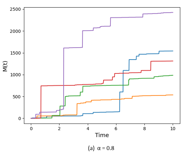
(a)

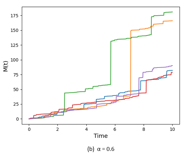
(b)

Figure 1: The sample paths for the ML Levy Subordinator.

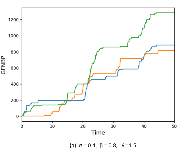
(a)

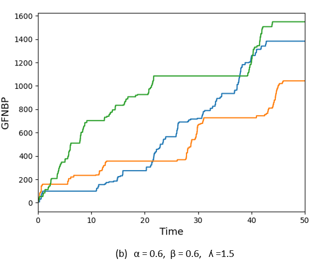
(b)

Figure 2: The sample paths for the GFNBP.

Declaration of competing interest

The authors declare that they have no known competing financial interests.

Data availability

No data was used for the research described in the article.

References

• Avramidis et al. (2003) A. N. Avramidis, P. L Ecuyer, P.-A. Tremblay, et al. Efficient simulation of gamma and variance-gamma processes. In Winter Simulation Conference, volume 1, pages 319–326, 2003.
• Barndorff-Nielsen (2000) O. E. Barndorff-Nielsen. Probability densities and Levy densities. University of Aarhus. Centre for Mathematical Physics and Stochastics …, 2000.
• Beghin (2015) L. Beghin. Fractional gamma and gamma-subordinated processes. Stochastic Analysis and Applications, 33(5):903–926, 2015.
• Beghin and Macci (2014) L. Beghin and C. Macci. Fractional discrete processes: compound and mixed poisson representations. Journal of Applied Probability, 51(1):19–36, 2014.
• Beghin and Vellaisamy (2018) L. Beghin and P. Vellaisamy. Space-fractional versions of the negative binomial and polya-type processes. Methodology and Computing in Applied Probability, 20(2):463–485, 2018.
• Biard and Saussereau (2014) R. Biard and B. Saussereau. Fractional poisson process: long-range dependence and applications in ruin theory. Journal of Applied Probability, 51(3):727–740, 2014.
• Cahoy et al. (2010) D. O. Cahoy, V. V. Uchaikin, and W. A. Woyczynski. Parameter estimation for fractional poisson processes. Journal of Statistical Planning and Inference, 140(11):3106–3120, 2010.
• Cook and Wei (2003) R. J. Cook and W. Wei. Conditional analysis of mixed poisson processes with baseline counts: implications for trial design and analysis. Biostatistics, 4(3):479–494, 2003.
• Cox and Lewis (1966) D. R. Cox and P. A. Lewis. The statistical analysis of series of events. 1966.
• Gorenflo and Mainardi (2015) R. Gorenflo and F. Mainardi. On the fractional poisson process and the discretized stable subordinator. Axioms, 4(3):321–344, 2015.
• Grandell (1997) J. Grandell. Mixed poisson processes, volume 77. CRC Press, 1997.
• Guler Dincer et al. (2022) N. Guler Dincer, S. Demir, and M. O. Yalçin. Forecasting covid19 reliability of the countries by using non-homogeneous poisson process models. New Generation Computing, pages 1–22, 2022.
• Ken-Iti (1999) S. Ken-Iti. Lévy processes and infinitely divisible distributions. Cambridge university press, 1999.
• Kilbas et al. (2002) A. A. Kilbas, M. Saigo, and J. J. Trujillo. On the generalized wright function. Fractional Calculus and Applied Analysis, 5(4):437–460, 2002.
• Kumar et al. (2019) A. Kumar, N. Upadhye, A. Wylomanska, and J. Gajda. Tempered mittag-leffler levy processes. Communications in Statistics-Theory and Methods, 48(2):396–411, 2019.
• Kumar et al. (2020) A. Kumar, N. Leonenko, and A. Pichler. Fractional risk process in insurance. Mathematics and Financial Economics, 14:43–65, 2020.
• Laskin (2003) N. Laskin. Fractional poisson process. Communications in Nonlinear Science and Numerical Simulation, 8(3-4):201–213, 2003.
• Laskin (2009) N. Laskin. Some applications of the fractional poisson probability distribution. Journal of Mathematical Physics, 50(11):113513, 2009.
• Maheshwari (2023) A. Maheshwari. Tempered space fractional negative binomial process. Statistics & Probability Letters, 196:109799, 2023.
• Maheshwari and Vellaisamy (2016) A. Maheshwari and P. Vellaisamy. On the long-range dependence of fractional poisson and negative binomial processes. Journal of Applied Probability, 53(4):989–1000, 2016.
• Maheshwari and Vellaisamy (2019a) A. Maheshwari and P. Vellaisamy. Fractional poisson process time-changed by lévy subordinator and its inverse. Journal of Theoretical Probability, 32(3):1278–1305, 2019a.
• Maheshwari and Vellaisamy (2019b) A. Maheshwari and P. Vellaisamy. Non-homogeneous space-time fractional poisson processes. Stochastic Analysis and Applications, 37(2):137–154, 2019b.
• Mathai et al. (2009) A. M. Mathai, R. K. Saxena, and H. J. Haubold. The H-function: theory and applications. Springer Science & Business Media, 2009.
• Meerschaert et al. (2011) M. Meerschaert, E. Nane, and P. Vellaisamy. The fractional poisson process and the inverse stable subordinator. Electronic Journal of Probability, 16:1600–1620, 2011.
• Meerschaert and Scheffler (2004) M. M. Meerschaert and H.-P. Scheffler. Limit theorems for continuous-time random walks with infinite mean waiting times. Journal of applied probability, 41(3):623–638, 2004.
• Meerschaert and Straka (2013) M. M. Meerschaert and P. Straka. Inverse stable subordinators. Mathematical modelling of natural phenomena, 8(2):1–16, 2013.