3D hydrodynamic simulations of massive main-sequence stars. III. The effect of radiation pressure and diffusion leading to a 1D equilibrium model

Abstract

We present 3D hydrodynamical simulations of core convection with a stably stratified envelope of a 25 $\mathrm{M}_{\odot}$ star in the early phase of the main-sequence. We use the explicit gas-dynamics code PPMstar which tracks two fluids and includes radiation pressure and radiative diffusion. Multiple series of simulations with different luminosities and radiative thermal conductivities are presented. The entrainment rate at the convective boundary, internal gravity waves in and above the boundary region, and the approach to dynamical equilibrium shortly after a few convective turnovers are investigated. From the results of these simulations we extrapolate to find the entrainment rate at the nominal heating rate and thermal diffusion given by the MESA stellar evolution model on which the 3D stratification is based. Further, to study the effect of radiative diffusion on the thermal timescale, we perform very long simulations accelerated by 10000 times their nominal luminosities. In these simulations the growing penetrative convection reduces the initially unrealistically large entrainment. This reduction is enabled by a spatial separation that develops between the entropy gradient and the composition gradient. The convective boundary moves outward much more slowly at the end of these simulations. Finally, we present a method to predict the extent and character of penetrative convection beyond the Schwarzschild boundary. This method is intended to be ultimately deployed in 1D stellar evolution calculations and is based on the properties of penetrative convection in our simulations carried forward through the local thermal timescale.

1 Introduction

Convective transport can be very efficient in stellar interiors, owing to the high energy densities there (Kippenhahn et al., 1990). At the convective-radiative boundary, it can play a crucial role in mixing chemical species (e.g. Denissenkov et al., 2012, in novae). Yet convection is one major uncertainty in the 1D stellar evolution model (e.g. Sukhbold & Woosley, 2014; Davis et al., 2018; Kaiser et al., 2020, in massive stars), with a set of parameters to calibrate to match with the observations (e.g. Schaller et al., 1992; Ribas et al., 2000; Trampedach et al., 2014; Tkachenko et al., 2020; Higl et al., 2021). For example, the efficiency of convective boundary mixing (CBM) during the main-sequence directly affects the model’s brightness and main-sequence lifetime (Salaris & Cassisi, 2017; Higgins & Vink, 2019). The local theory of convection, mixing-length theory (MLT) formalized by Böhm-Vitense (1958) and Cox & Giuli (1968) is widely used in 1D stellar evolution codes (e.g. Paxton et al., 2010). Other sophisticated theories on convection have also been proposed. For example, Xiong (1986) developed a non-local MLT that indicates penetrative convection. Pasetto et al. (2014) removes the mixing length in their convection theory. A spectrum of turbulent eddies instead of a typical rising blob is considered in Canuto & Mazzitelli (1991).

Convection is not only an important mechanism to transport energy and species, but also excites internal gravity waves (IGWs) (Lecoanet & Quataert, 2013; Pinçon et al., 2016). It is predicted theoretically that radiative diffusion damps travelling IGWs, which carry angular momentum(Rogers & McElwaine, 2017; Aerts et al., 2019). This process leads to deposition of angular momentum where the IGWs are damped, and hence to redistribution of angular momentum (Zahn et al., 1997). Asteroseismological observations help constrain convective boundary mixing and diffusive mixing in the radiative envelope (Moravveji et al., 2015; Michielsen et al., 2019, 2021).

Penetrative convection has been investigated in theory and through numerical simulations for decades in various contexts, core convections and shell convections for exapmle (Roxburgh, 1989; Arnett et al., 2015; Anders et al., 2022; Korre & Featherstone, 2021; Blouin et al., 2023). The extent of convective penetration and its dependence on various properties of the Schwarzschild boundary (SB) have been studied (Hurlburt et al., 1994; Baraffe et al., 2021). The temperature gradient in the convective boundary (CB) region may be deduced by asteroseismological observation and modeling (Michielsen et al., 2021). Current treatment of the convective boudary in 1D stellar evolution simulations includes f overshooting (Herwig et al., 2000), instantaneous overshooting (Maeder, 1976) and entrainment (Staritsin, 2013; Scott et al., 2021). In this work, we define the SB to be the location where the rising radiation diffusion energy flux as we go outward in radius in the core convection zone first equals the total luminosity. We find that this is not the location where the entropy gradient first becomes positive and the temperature gradient first becomes subadiabatic, as we will discuss later. Beyond the SB we have a region of penetrative convection leading up to the CB. We here define the CB to be that radius at which the radiative energy flux becomes equal to the total luminosity, the convective entropy flux vanishes, and also the turbulent dissipation of kinetic energy of the convection flow vanishes.

Previously, in the first paper of this series, we have introduced the general properties of core-convection simulations of a 25 $\mathrm{M}_{\odot}$ star approximated with an ideal gas equation of state (Herwig et al., 2023, Paper I). We confirmed earlier results of massive main-sequence star simulations by Meakin & Arnett (2007) and Gilet et al. (2013). These authors reported entrainment rates of envelope material into the convective core that are orders of magnitude larger than what is compatible with stellar models and basic observational properties. Candidate physical mechanisms that may impact the entrainment rate in hydrodynamic simulations include a more realistic thermodynamic stratification, radiative diffusion, rotation and magnetic fields.

The properties of IGWs in our 3D PPMstar ideal gas simulations are presented in (Thompson et al., 2023, Paper II). One important aspect of IGWs excited by core convection is the possibility that they may cause material or angular momentum mixing in the radiative layer. Radiative diffusion permits the entropy in the stably stratified envelope to no longer be a constant of the motion. As a consequence, irreversible envelope mixing becomes possible, even though IGW velocity amplitudes are damped by radiative diffusion. Our strategy in this paper is to study the impact of radiation pressure and radiative diffusion on the convection zone in our model star and on the structure of the CB region. We will analyze the spectrum of IGWs that are excited at the CB for the purpose of comparison with the studies of Paper I and Paper II in this series, but we will leave the issue of potential material mixing in the envelope to a forthcoming paper.

The main goals of this work are as follows: to test whether adopting a more realistic simulation approach which includes radiation pressure and diffusion can reduce the entrainment rate significantly; to study the effect of radiative diffusion on the spectrum of IGWs in the stable envelope; to investigate the stratification of penetrative convection and develop a method to predict the convective penetration depth.

The first 3 sections discuss flow phenomena on a short timescale (convective timescale) and the following two sections investigate the growing penetrative convection on a thermal timescale. Finally, we discuss our results and conclusions in the last section. Specifically, in §2 we present the simulation method, simulation setup, and assumptions. Section §3 describes the general flow dynamics from the onset of core convection to a 3D quasi-steady state on a convective timescale, introduces the CBM, excitation of IGWs and their power spectra, and discusses the effect of radiative diffusion on the CBM and IGWs along the way. In §4, the long-time behaviors of stellar stratification and convective penetration are discussed. The gradual development of the penetration region beyond the SB is observed in a very long duration simulation. In this simulation the development of a positive entropy gradient in the penetration region that is sustained despite efficient species mixing is identified as a key structure that acts to bring the intensity of convective motions down, so that further entrainment and outward motion of the convective boundary is greatly reduced. In §5, a method to predict the penetration depth and the stratification within the penetration region is presented in terms of a 1-D model of the core convection zone that can be worked out if the kinetic energy dissipation rate up to the SB has either been determined from a short 3-D simulation on a modest grid or has been approximated by interpolating between such simulations under similar conditions. We summarize and discuss our main results and conclusions in §6.

2 Methods and assumptions

To study the effect of radiation, we apply the equation of state that includes radiation pressure in addition to that of a monatomic gas. This allows direct application of the MESA (Paxton et al., 2010, 2013, 2015) model with minimal fitting and approximation in going from 1D to 3D initialization. The base state is constructed from the 25 $\mathrm{M}_{\odot}$MESA stellar evolution model (Davis et al., 2018) $1.64\times 10^{6}$$\mathrm{yr}$ after the start of H burning on the zero-age main sequence. The exponential CBM model is used. In this model, the region outside the SB obeys the radiative temperature gradient. Details on the 1D model can be found in Paper I. Fig. 1 shows the agreement of radial profiles of the initial state on the 3D Cartesian grid with the MESA model.

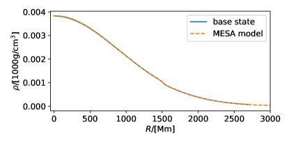
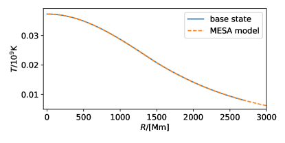
Figure 1: Comparison of adopted base state for the 3D simulations and the MESA radial profile of density and temperature. Quantities are given in their code units.

We use the PPMstar gas dynamics code described in Woodward et al. (2015) and applied in Woodward et al. (2015); Jones et al. (2017); Andrassy et al. (2020). The PPMstar tracks the H rich materials in the stable envelope by fractional volume $f_{\rm V}$, and materials in the convective core by $1-f_{\rm V}$. In this version, the contribution of radiation is included in the internal energy per unit mass $e$, pressure $p$ and specific entropy $s$

$$e(\rho,T,\mu) = \frac{RT}{(\gamma-1)\mu}+\frac{aT^{4}}{\rho}$$ (1)

$$p(\rho,T,\mu) = \frac{R\rho T}{\mu}+\frac{aT^{4}}{3}$$ (2)

$$s(\rho,T,\mu) = -\frac{R}{\mu}\ln\rho+\frac{R}{(\gamma-1)\mu}\ln T+\frac{4aT^{3}}{3\rho},$$ (3)

where $\mu$ is the mean molecular weight,$\rho$ density, $T$ temperature, $R$ gas constant, $\gamma=5/3$, $a$ radiation constant. The technique of model equation of state (Woodward, 1986) is applied,

$$p=p_{00}+(\tilde{\gamma}-1)\rho\varepsilon$$ (4)

the coefficients $p_{00}$ and $\tilde{\gamma}$ of which are different in each grid cell, that preserves sound speed $c_{s}$ and energy density $\rho\varepsilon$ every time step

$$\tilde{\gamma}=1+\frac{c_{s}^{2}\rho}{p+\varepsilon\rho},\ p_{00}=p-(\tilde{\gamma}-1)\rho\varepsilon.$$ (5)

The radiative flux,

$$\bm{F}=-k\nabla T$$ (6)

is implemented explicitly in PPMstar as a part of the energy flux in every time step update, with radiative thermal conductivity (Kippenhahn et al., 1990)

$$k=\frac{4acT^{3}}{3\kappa\rho},$$ (7)

where $\kappa$ is the opacity, $c$ speed of light. Simulations from M200 to M213 (see Table 1) use the following opacity fit as a function of hydrogen mass fraction and temperature:

$$\kappa = \min(\frac{c_{es}10^{\sum_{i=0}^{3}(a_{i}(\log_{10}T)^{3-i})}}{\kappa_{\rm min}c_{\rm corr}},\kappa_{\rm tot})$$ (8)

$$c_{\rm es} = 0.2(1+x_{\rm H})$$

$$c_{\rm corr} = 1+0.5(\frac{\kappa_{\rm max}}{\kappa_{\rm min}}-1)(1-\tanh(w\log_{10}\frac{T}{T_{0}}))$$

where $x_{\rm H}$ is hydrogen mass fraction, $\kappa_{\rm min}$, $\kappa_{\rm max}$, $\kappa_{tot}$, $a_{i}$, $T_{0}$ and $w$ are fitting parameters.

Simulations M284, M250, M251 and M252 use another opacity fit to the OPAL opacity (Iglesias & Rogers, 1996) as a function of density, temperature and hydrogen mass fraction:

$$\kappa=\sum_{i=0}^{5}a_{i}(t_{7})^{5-i}{}$$ (9)

In Eq. 9, $t_{7}=\log_{10}T-7$ and

$$a_{i}=w_{11}a^{i}_{11}+w_{12}a^{i}_{12}+w_{21}a^{i}_{21}+w_{22}a^{i}_{22}$$

$$w_{11}=(r_{2}-r)(x_{2}-x_{h})/((r_{2}-r_{1})(x_{2}-x_{1}))$$

$$w_{12}=(r_{2}-r)(x_{h}-x_{1})/((r_{2}-r_{1})(x_{2}-x_{1}))$$

$$w_{21}=(r-r_{1})(x_{2}-x_{h})/((r_{2}-r_{1})(x_{2}-x_{1}))$$

$$w_{22}=(r-r_{1})(x_{h}-x_{1})/((r_{2}-r_{1})(x_{2}-x_{1}))$$

$$r=\log_{10}\rho-3\log_{10}T+21$$

where $x_{1}$, $x_{2}$, $r_{1}$, $r_{2}$, $a^{i}_{jk}$ are fitting parameters.

We apply a reflecting boundary condition at radius 2670 $\mathrm{Mm}$, and make the heat fluxes at opposite cell interfaces equal for 3 grid cell widths inside this reflecting sphere. We perform a series of $25\mathrm{M}_{\odot}$ simulations (Table 1), with varying driving luminosities and radiative thermal conductivity $k$. Properties such as the mass entrainment rate at the CB at the nominal luminosity are extrapolated from simulations with boosted luminosities. For a luminosity boosting factor $X$, we have cases with 0, $X^{2/3}$ and $X$ boosting factors for radiative diffusion. Henceforth, we refer to them by no diffusion, intermediate diffusion, and high diffusion.

3 From the initial transient to a quasi-steady 3D flow

Here we briefly describe the dynamics of the initial transient which takes place for the first few convective turn-overs from time 0, and the following quasi-steady 3D flow. In our many cases considered here, we find that the visualization looks qualitatively similar regardless of the boosting factor for luminosity and radiative diffusion. See our representative simulation M252 (luminosity and radiative diffusion boosted by a factor of 10000) at https://ppmstar.org. In the discussion below, we will point out the effect of radiative diffusion when it matters qualitatively and quantitatively.

3.1 The development of the fully convective core

At time 0, the initial state is in perfect hydrostatic equilibrium. The radiative diffusion is transporting heat according to the stratification and opacity. As in Paper I  the nuclear burning is emulated as a time-independent Gaussian volume heating $\sim\exp(-r^{2}/(2\sigma^{2}))$, $\sigma=280\,\mathrm{Mm}$. Given the temperature gradient, there is the excess heat in the core accumulating due to insufficient radiative energy transport. The center of the core becomes convectively unstable as a result. The central gas parcels rise because of the buoyancy force and thereby convection starts. Because the convective core is almost adiabatic, the moving fluid elements move effortlessly on the same adiabat. The excess heat unable to be carried by the radiative diffusion is now transported by the emerging convection within the core until the rising, relatively buoyant fluid elements encounter the positive entropy gradient where the stratification becomes convectively stable.

Once the rising plumes encounter the entropy gradient, the buoyancy force restrains them from going further outward in radius. The interaction between the plumes and the convective-radiative boundary excites IGWs that propagate in the stable envelope. During the first few convective turnovers, the core convection becomes fully turbulent and excites IGWs of a broad range of wavelengths. An analysis of the power spectrum of the IGWs in the stable envelope after the initial transient adjustment of the flow to its 3D degrees of freedom is presented at the end of this section.

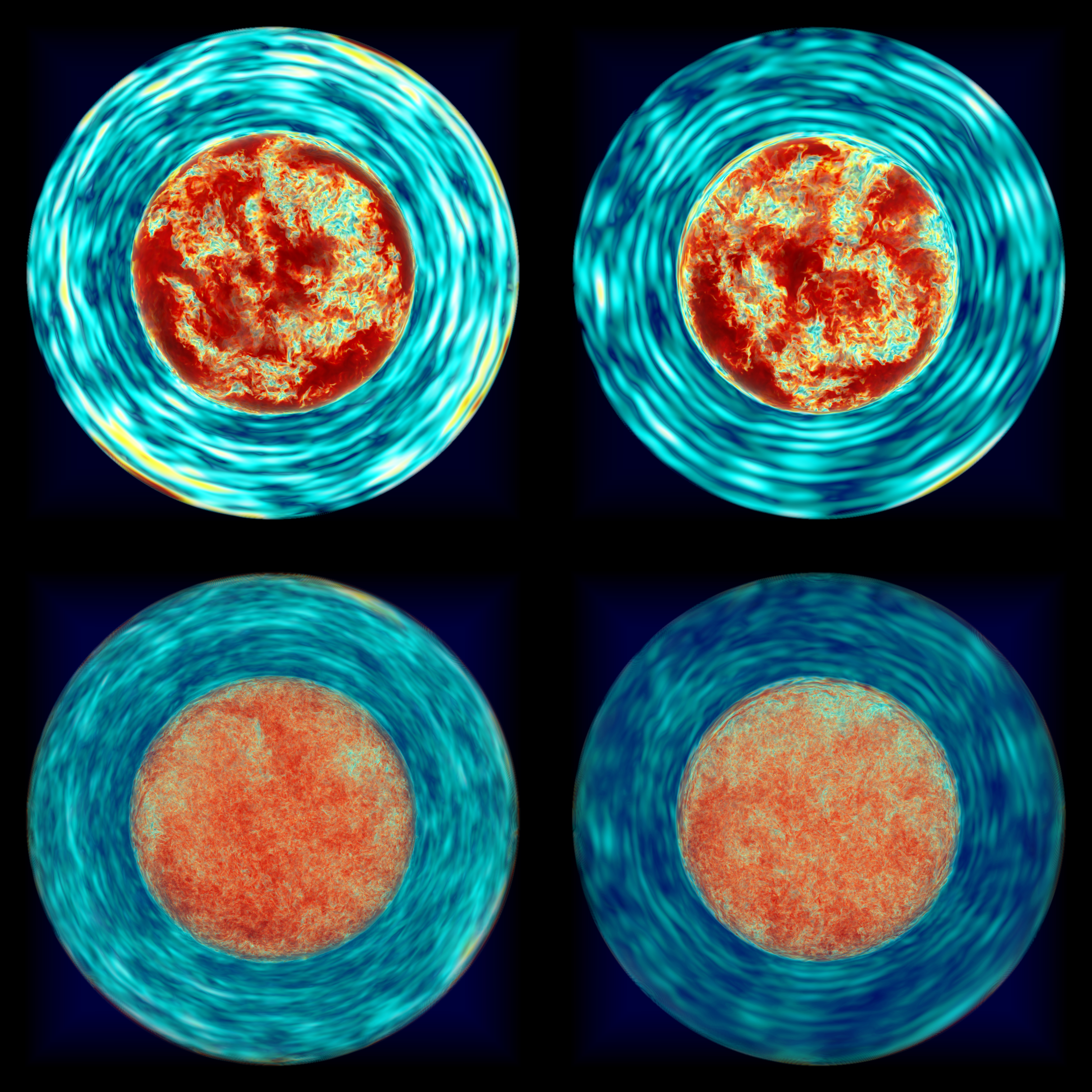
Figure 2: Images of a thin slice through the center of the star of the horizontal velocity component (top row) of M201 (left column, no radiative diffusion) and M207 (right column, 1000x radiative diffusion), and of the vorticity magnitude (bottom row). Movies of these quantities are available at https://ppmstar.org.

Table 1: Simulation summary providing the run ID, the grid, luminosity $L$ boosting factor, thermal conductivity $k$ boosting factor, end time of the run, and entrainment rate, $*$ denotes values from the MESA model. The runs labelled by $\dagger$ are long-duration, the entrainment rates of which decline over time. Hence we fit them by a straight line from dump 5000 to 6000 to compute the corresponding entrainment rates.

ID	grid	$L/L_{*}$	$K/K_{*}$	$t_{\mathrm{end}}/{\rm h}$	$\dot{M}/[\mathrm{M}_{\odot}\ \mathrm{yr}^{-1}]$
M200	$768^{3}$	1000.0	0.0	1817.6	$6.82\times 10^{-1}$
M201	$1152^{3}$	1000.0	0.0	3556.3	$6.85\times 10^{-1}$
M202	$1152^{3}$	100.0	0.0	2439.2	$3.60\times 10^{-2}$
M203	$1152^{3}$	3162.0	0.0	1468.1	$2.41\times 10^{0}$
M204	$1152^{3}$	1000.0	100.0	3362.9	$6.53\times 10^{-1}$
M205	$1152^{3}$	100.0	21.5	2648.4	$3.91\times 10^{-2}$
M206	$1152^{3}$	3162.0	215.4	1549.8	$2.16\times 10^{0}$
M207	$1152^{3}$	1000.0	1000.0	3838.4	$3.69\times 10^{-1}$
M208	$1152^{3}$	100.0	100.0	2446.4	$2.00\times 10^{-2}$
M209	$1152^{3}$	3162.3	3162.3	1465.3	$1.36\times 10^{0}$
M210	$1728^{3}$	1000.0	1000.0	3495.3	$3.91\times 10^{-1}$
M211	$768^{3}$	1000.0	100.0	2089.7	$6.31\times 10^{-1}$
M212	$1152^{3}$	31.62	31.62	2297.4	$6.03\times 10^{-3}$
M213	$768^{3}$	1000.0	1000.0	3537.5	$3.72\times 10^{-1}$
M284	$2688^{3}$	1000.0	1000.0	3418.4	$3.38\times 10^{-1}$
M250†	$896^{3}$	3162.3	3162.3	20769.0	$5.77\times 10^{-1}$
M251†	$896^{3}$	1000.0	1000.0	18444.4	$1.74\times 10^{-1}$
M252†	$896^{3}$	10000.0	10000.0	25137.6	$1.40\times 10^{-1}$

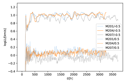
Figure 3: The overall magnitude of horizontal velocities 0.5 $H_{p}$ below and above the $N^{2}$ peak (see Eq. 10 ) becomes constant after an initial transient (400 hours) when we average over the persistent fluctuations.

The convective core soon develops the characteristic dipole circulation pattern that was first seen in the 3D simulations of Porter et al. (2000). It has been noted by many investigators that convection tends to develop convection cells that extend to the largest vertical scale (Hurlburt et al., 1986; Freytag et al., 1996; Porter et al., 2000; Andrassy et al., 2022). In Fig. 2, when the dipole plume hits the CB and diverges, the flows become mostly horizontal near the boundary, bringing along buoyant materials from the boundary. Entrainment of the fluid from the stable layer into the convection zone is facilitated by the boundary layer separation (Woodward et al., 2015). We define dynamical equilibrium as a state in which the kinetic motions, charaterized by kinetic energy density, buyoancy driving, work by pressure field, become statistically time-independent on the convective timescale, demonstrated by the horizontal velocity in Fig. 3. While in dynamic equilibrium the mass entrainment rate decreases as the simulation approaches a state closer to thermal equilibrium. The entrainment analysis can be found in §3.3 using the same methodology as in Paper I.

In stellar evolution models the CB is usually defined as the radius at which the adiabatic gradient is equal to the radiative gradient, also known as the SB. Based on our discussion of a very long-duration simulation in §4, we choose to define the CB in this work as the radius where, in statistical dynamical and thermal equilibrium, the radial derivatives of the radiative and convective heat fluxes as well as the convective heat flux itself and the kinetic energy dissipation rate all vanish. The CB, thus defined, is different from the SB, because at the SB the radial derivative of the radiative heat flux does not vanish.

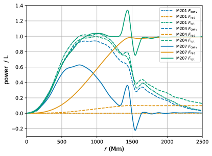
Figure 4: Total convective (radiative) energy flux for the no-diffision (M201, 0x), intermediate-diffusion (M204, 100x) and high diffusion (M207, 1000x) simulations with 1000x luminosity enhancement at dump 3500. The curves are smoothed by using moving averages three times over a window 120 $\mathrm{Mm}$ wide and time-averaged over 100 dumps $\sim\ 140\ \mathrm{hr}$. The fluxes are defined in Eq. 11 and Eq. 12. Temperature, opacity, and density in Eq. 12 are spherical averages.

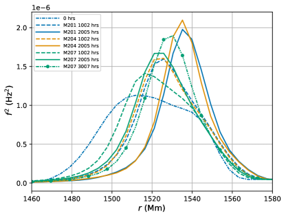
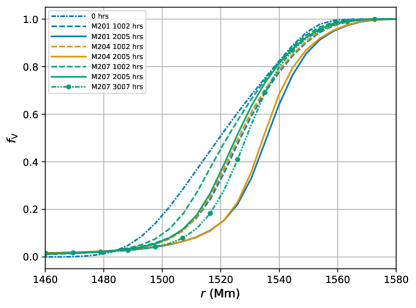
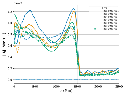
Figure 5: Profiles of $N^{2}$, $f_{\rm V}$, $|U_{t}|$ of the simulations with 1000x luminosity enhancement (M201: no diffusion, M204: $K\sim L^{2/3}$, M207: $K\sim L$, all at the $1152^{3}$ grid resolution.)

3.2 Dynamics and kinematics in dynamical equilibrium

The convection rapidly organizes itself such that the total convective flux becomes the luminosity minus the total radiative energy flux (Fig. 4, Eq. 11, Eq. 12). Therefore, our simulated star reaches a dynamical equilibrium over the first few convective turn-overs and stays in dynamical equilibrium thereafter.

3.2.1 Effect of radiative diffusion

Fig. 5 shows how $f_{\rm V}$, tangential velocity, and the Brunt-Väisälä (BV) frequency squared $N^{2}$, Eq. 10, evolve for different strengths of radiative diffusion at 1000x the nominal luminosity.

$$N^{2}=\frac{g\delta}{H_{p}}(\nabla_{\mathrm{ad}}-\nabla_{\rm star})+\frac{g\delta}{H_{p}}\frac{\phi}{\delta}\nabla_{\mu}\equiv N_{t}^{2}+N_{\mu}^{2}{}$$ (10)

where

$$\delta=-(\frac{\partial ln\rho}{\partial lnT})_{p,\mu},\phi=(\frac{\partial ln\rho}{\partial ln\mu})_{p,T}$$

$$\nabla_{\rm star}=\frac{dlnT}{dlnp},\nabla_{\mathrm{ad}}=(\frac{dlnT}{dlnp})_{S},\nabla_{\mu}=\frac{dln\mu}{dlnp}$$

and $\rho$ is density, T temperature, $H_{p}$ pressure scale height, $\mu$ mean molecular weight, $S$ specific entropy, $\nabla_{\rm star}$ the actual temperature gradient, $\nabla_{\mathrm{ad}}$ the adiabatic gradient, and $\nabla_{\rm star}-\nabla_{\mathrm{ad}}$ is the superadiabaticity. Outward from the SB by about 120 $\mathrm{Mm}$ ($10\%$ in radius) in the initial state of the simulation, $N^{2}$ has a strong, slowly migrating peak reflecting the sudden change of entropy mainly caused by the change in $\mu$ at that location.

Perhaps the most important effect of the radiative diffusion is that, as this is increased, the position of the composition change, traced by the $f_{\rm V}$ profile, moves outward less rapidly. This effect can also be seen in the position of the $N^{2}$ peak feature. This behavior can be explained by the fact that when we add radiative diffusion, we introduce into the problem a mechanism for carrying the heat introduced into the convection zone outward through the stably stratified envelope. In the absence of this mechanism, in addition to entraining high entropy materials from the envelope, heat must pile up in the convection zone, and this must cause it to expand. This is analogous to the helium shell flash in that the ignition of helium fusion in a thermal pulse produces more energy temporarily than can be carried away by radiative diffusion, causing the star to expand and brighten (Herwig et al., 2006). In our high diffusion case, heating by nuclear burning is on average, removed by the heat energy flowing through the reflecting sphere at our outer boundary in the form of radiation (Fig. 4). The total convective flux and total radiative energy flux are calculated by Eq. 11 and Eq. 12.

$$F_{\mathrm{conv}}(r)=\iint\limits_{\mathrm{sphere}\ r}(p+\rho e+\frac{1}{2}\rho u^{2})u_{r}dA{}$$ (11)

$$F_{\mathrm{rad}}(r)=-\frac{4\pi r^{2}c}{3\kappa\rho}\frac{\partial(aT^{4})}{\partial r}{}$$ (12)

The convective flux is the flux of enthalpy plus the kinetic energy summed over the sphere at radius $r$. $c$ is the speed of light and $\kappa$ is the opacity.

In cases of no diffusion, there is no diffusive heat flux across the stably stratified gas in the outer part of our computational region. The heated convective core pushes the envelope resulting in positive convective flux at all radii. We measure that about $55\%$ of the nuclear heating becomes potential energy by expanding the convective core and compressing the stable envelope (i.e. redistributing mass in a static gravitational potential), while $45\%$ becomes internal energy by heating the star up. In the intermediate diffusion case M204, $42\%$ of the nuclear heating expands the core and $46\%$ heats the star up. About $10\%$ of the nuclear heating is transported outward by radiative diffusion in that case. In Fig. 5, the convective velocity is slightly smaller in the high diffusion case but the profile of the tangential velocity remains similar. In all cases, the kinetic energy is negligible, once a dynamical equilibrium is established, it mostly does not change over time and stays negligible. The effect on the motion in the stable envelope, i.e., IGWs, is discussed in §3.

The differences in the heights and shapes of the $N^{2}$ peaks, between the cases of no diffusion and intermediate diffusion at the same time (1000 or 2000 hours), are very small (Fig. 5), because most of the heat injected (90% and 100%) piles up in the convective core which leads to quantitatively similar dynamics. However, in the case of high diffusion, the change of location and shape in the $N^{2}$ peak is noticeably smaller than in the other two cases given the same amount of time (Fig. 5). However, the overshoot and undershoot of the convective flux, and the overshoot of radiative flux at 1500 $\mathrm{Mm}$ suggest the thermal structure is adjusting, at a small rate. Hence, any significant change in the stratification for the high diffusion cases happens on a longer timescale than no or intermediate diffusion. To reduce the computational cost of studying the evolution on a longer timescale, we investigate the effect of enhancing luminosity in the next section and the possibility of accelerating the evolution by enhancing the luminosity in §4.

The heat piling up in the no or intermediate diffusion cases explains the fact that the star lifts the convective core and compresses the envelope. This process will continue and completely change the stratification because the total energy of our simulation keeps increasing in these two cases. Hence, to simulate a realistic star in thermal equilibrium, the only reasonable scenario is the high diffusion one, and we later discuss the effect of enhancing luminosity using the high diffusion cases only. In addition, as discussed in §3.3, the entrainment continues at a relatively constant rate, which suggests that the star is still adjusting its stratification and has not yet reached a thermal equilibrium. In such an equilibrium, all the temporal dependence on time scales longer than several large eddy turn-overs in the convection zone could be expected to very nearly vanish. By definition, the total heat content will be radiated away at the rate of the luminosity on a thermal timescale, if there is no nuclear heating. Therefore, it is not feasible to investigate the dynamics on a thermal timescale in the cases of no or intermediate diffusion without disrupting the thermodynamical structure completely. Hence, the discussion on the evolution on a thermal timescale in §4 and §5 focusses on the high diffusion cases.

3.2.2 Effect of enhancing luminosity

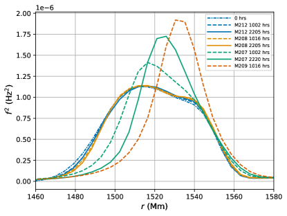
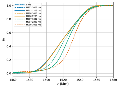
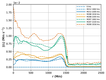
Figure 6: Profiles of $N^{2}$, $f_{\rm V}$, $|U_{t}|$ of M212 (31.62x $L_{*}$ & $K_{*}$), M208 (100x $L_{*}$ & $K_{*}$), M207 (1000x $L_{*}$ & $K_{*}$), M209 (3162x $L_{*}$ & $K_{*}$), all at the $1152^{3}$ grid resolution.

Fig. 6 shows the profiles of $N^{2}$, $f_{\rm V}$, and horizontal velocity for a series of runs in which we vary the luminosity. For each boosting factor, we also enhance the radiative diffusion by the same factor. Cases of enhancement factors of 31.62, 100, 1000, and 3162 are used. For the two lowest luminosity cases, we observed essentially no change within 2000 hours in the profile of $f_{\rm V}$, and in the position and the shape of the $N^{2}$ peak during these simulations. This certainly does not mean that changes would not result were these two simulations run longer in time.

Runs M207 and M209, with luminosity enhancement factors of 1000 and 3162, reshape the initial $f_{\rm V}$ radial profile within relatively short times of less than 2500 hours. After this intial reshaping in these high-power cases, the $f_{\rm V}$ radial profile translates while maintaining its shape as the gas from above the convection zone is entrained. As will be discussed in §4, boosting the nuclear heating and the radiative diffusion by a common factor can be regarded as accelerating the time rate of change of the stellar model. In order to probe the long-time behavior of the stellar model, this balanced enhancement of the luminosity and radiation diffusion is appealing for our explicit PPMstar code, because it dramatically lowers the cost of finding the long-time behavior.

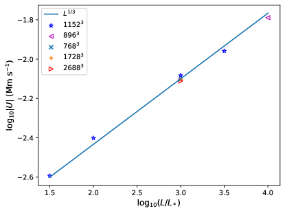
Figure 7: Luminosity versus convective velocity magnitude in the convection zone at 1000 $\mathrm{Mm}$ averaged over 20 dumps. All cases are high diffusion.

Fig. 7 confirms that the magnitude of velocity scales with $L^{1/3}$ in the presence of radiation pressure and radiative diffusion. This scaling is also observed in Paper I.

3.2.3 Convergence

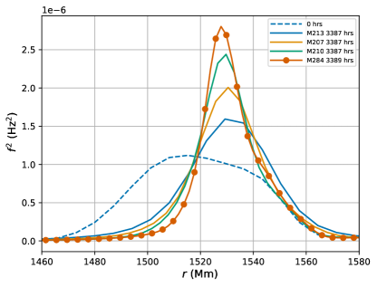
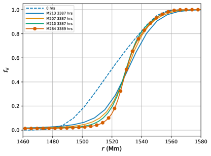
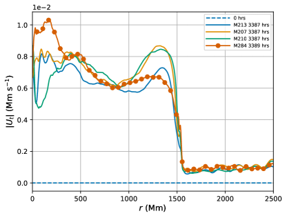
Figure 8: Snapshots of $N^{2}$, $f_{\rm V}$, $|U_{t}|$ of M213: $768^{3}$, M207: $1152^{3}$, M210: $1728^{3}$, M284: $2688^{3}$, all with 1000x $L_{*}$ and 1000x $K_{*}$.

In Fig. 8, the profiles of $N^{2}$, $f_{\rm V}$ and horizontal velocity are presented for a sequence of simulations carried out at different grid resolutions to show the effect of refining our computational grid. These simulations are performed with a luminosity and radiation diffusion enhancement factor of 1000. We see that the $N^{2}$ peak becomes higher with increasing grid resolution. However, the location of the $N^{2}$ peak is roughly the same regardless of the resolution. The radial profile of $f_{\rm V}$ becomes steeper with grid refinement, and it is clear that this steepening is not complete even on the highest resolution grid shown in the figure. Although there is some statistical noise evident in the plots of the horizontal component of the velocity in Fig. 8, it is clear that these simulations have converged upon mesh refinement to a well-defined state. Even the radial profiles of $f_{\rm V}$ near the CB appear to have converged in terms of the position of the sharp increase in $f_{\rm V}$ though not in its steepness. The interpretation of the $N^{2}$ peak and the slope of the $f_{\rm V}$ not converging on grid refinement is that we have not converged on mixing. In §4, convergence will be shown for turbulent dissipation measured from the simulations and for vorticity in the stable envelope.

3.2.4 Mixing length parameter

We first check the efficiency of convection. The mean free path of a photon inside our star is of order of $1-10\ \mathrm{cm}$, i.e. our star is opaque and radiative transport of energy can be treated as a diffusion process. We take $r_{c}=1500\ \mathrm{Mm}$ as the radius of our convective core, the thermal adjustment timescale of the convective core will be $\tau_{K}=r_{c}^{2}/K$. The convective timescale is $\tau_{c}=2r_{c}/v_{c}\ .$ For our M207 case, the boosting factor for the radiative diffusion can be interpreted as decreasing the thermal conductivity by a factor of 1000. Given that,

$$\frac{\tau_{c}}{\tau_{K}}=\frac{2K}{v_{c}r_{c}}$$

is about $1.06\times 10^{-4}$. Therefore, the convection in our simulations is efficient in transporting excess heat. We measure the super-adiabatic temperature gradient in our simulations and hence can derive numerical values of the standard mixing length parameter $\alpha$.

In MLT, the total convective flux is

$$F_{\mathrm{conv}}=4\pi r^{2}\rho c_{p}\sqrt{p/\rho}(\nabla_{\rm star}-\nabla_{\mathrm{ad}})^{3/2}\alpha^{2}{}$$ (13)

where symbols have their usual meaning, is proportional to $\alpha^{2}$ (Prialnik, 2000).

From the superadiabaticity in Fig. 9, we see that the temperature gradient is nearly adiabatic throughout the convective core ($\nabla_{\rm star}-\nabla_{\mathrm{ad}}\sim\ 10^{-4}$). The convective core is slightly superadiabatic inside 1000 $\mathrm{Mm}$ and becomes slightly subadiabatic beyond 1000 $\mathrm{Mm}$. This is where the radial entropy gradient $dS/dr$ becomes positive and the convective flows start to encounter the marginally stable stratification. Though the convective stability criterion indicates the stratification is stable at 1000 $\mathrm{Mm}$ and outward, this slightly subadiabatic temperature gradient cannot bring the convetive motion to a halt. The flows continue before arriving at the very much more significant entropy gradient at the CB.

The convective flux is propotional to $(\nabla_{\rm star}-\nabla_{\mathrm{ad}})^{3/2}$. However, the temperature gradient is not superadiabatic throughout the entire convective core (Fig. 9). If we take the approach in Porter et al. (2000), redefining the superadiabaticity as $\nabla_{\rm star}-f\nabla_{\mathrm{ad}}$ where $f=0.999$, we find that the entire convective core is superadiabatic and the mixing length parameter $\alpha$, solved from Eq. 13, is in the range from 0.4 to 1.2 (Fig. 10). This value of $f$ is different from the value 0.98 used in Porter et al. (2000). Chan & Sofia (1989) suggest that the superadiabaticity might depend on the aspect ratio of the convective spherical shell and upon the equation of state. We find that $\nabla_{\rm star}-\nabla_{\mathrm{ad}}$ is positive inside 1000 $\mathrm{Mm}$ and negative beyond 1000 $\mathrm{Mm}$ for all our different heating rates, but its magnitude increases with the boosting factor. This is qualitatively in agreement with the MLT assertion that the convective flux scales with superadiabaticity to the power of $3/2$.

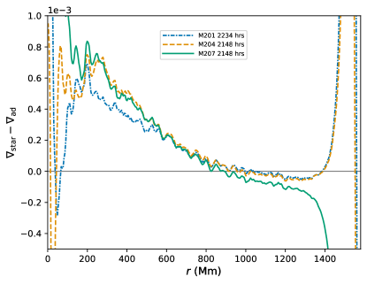
Figure 9: The superadiabaticity ($\nabla_{\rm star}-\nabla_{\mathrm{ad}}$) of M201 (1000x heating, 0x diffusion), M204 (1000x heating, 100x diffusion) and M207 (1000x heating, 1000x diffusion), averaged over 100 dumps and 30 $\mathrm{Mm}$.

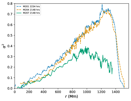
Figure 10: The mixing length parameter squared $\alpha^{2}$ of M201, M204, M207 averaged over 100 dumps and 30 $\mathrm{Mm}$.

3.3 Mass entrainment rate

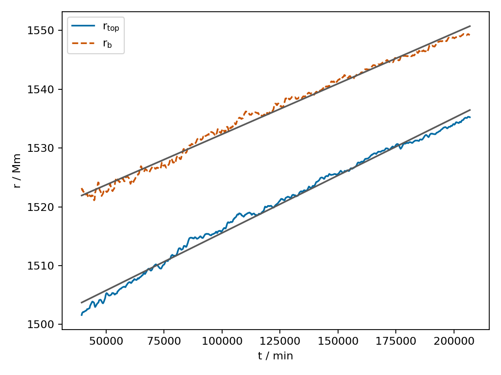
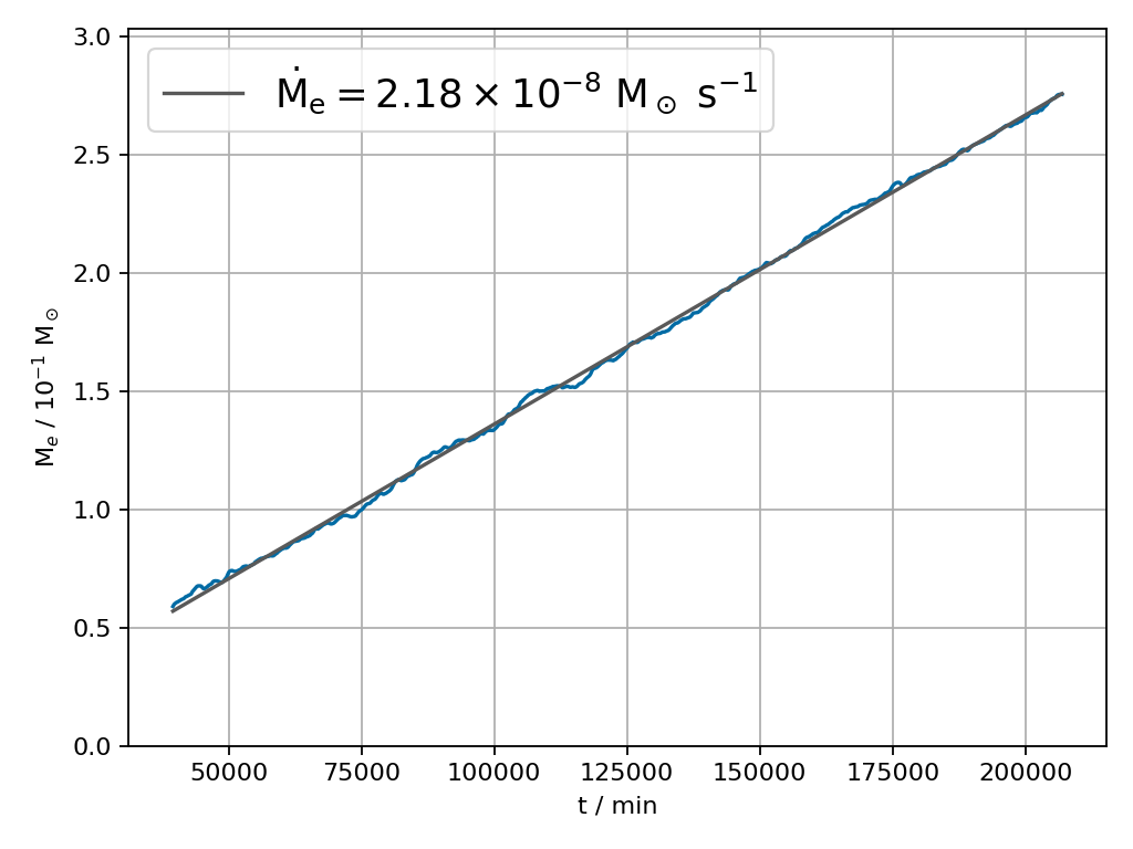
Figure 11: The time evolution of the radius of maximal $df_{\rm V}/dr$ minus one $f_{\rm V}$ scale height, and the entrained masses of M201.

We determine the entrainment rate of the envelope gas of from above the CB into the convection zone using the same methodology as in Paper I. As in Paper Iwe define the entrained mass as the total mass of the envelope material within $r_{b}$. $r_{b}$ is the location of the maximum gradient of $f_{\rm V}$ less one $f_{\rm V}$ scale height. This entrained mass evolves linearly with time, and one example is shown in Fig. 11.

Compared to the $P_{\mathrm{gas}}$ only case (M114 in Paper I) the entrainment rate is $14\%$ smaller when adding $P_{\mathrm{rad}}$ (M201), and decreases by $50\%$ when also adding radiative diffusion (M207).

We estimate the entrainment rate at nominal heating by extrapolating separately from three sets (no, intermediate and high diffusion) of simulations (Fig. 12). The entrainment rates for no diffusion and intermediate diffusion are practically the same. The difference between the entrainment rates extrapolated from these two sets are due to the uncertainty of the fitting slope.

The extrapolated entrainment rate cannot persist for a significant fraction of the main-sequence lifetime (§4). We believe instead that the large entrainment rates that we observe after our simulations initially establish a dynamical equilibrium, are the result of thermal non-equilibrium. We will discuss the development of penetrative convection on a longer time scale and the effect on the entrainment of the resulting subadiabatic temperature gradients within the penetrative region between the SB and the CB in §4 and §5

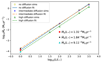
Figure 12: Entrainment rates of simulations (hollow symbols); extrapolated entrainment rates at nominal heating (solid symbols).

3.4 IGWs

One important consequence of radiative diffusion is damping of IGWs in the stably stratified layers of the star (Zahn et al., 1997). We study this effect of radiative diffusion in our model star by observing the wave motions in the envelope surrounding the convective core. Using the same approach as in Paper II, we decompose the radial component of the velocity field into complex spherical harmonics coefficients using the SHTools package (Wieczorek & Meschede, 2018). We then perform a Fourier transform on each coefficient time-series. Then we use the SHTools package to calculate the power spectral density of the radial velocity oscillations normalized by degree l for each frequency bin. The time interval between data dumps in our simulations determines an upper limit to the frequencies that we can observe. This upper limit is about 200 ${\rm\mu}$ $\mathrm{Hz}$ for the simulations reported here, corresponding to $\approx 43\ \mathrm{min}$ between dumps. In these simulations, we have located our outer boundary so that the radius of the convective core is about $60\%$ of the boundary radius. The $l$ index of the spherical harmonics gives the number of nodes going along a meridian from one pole to the other. Hence at the CB ($60\%$ of the maximal radius in our computational region), with a $1152^{3}$ grid, we can resolve, in principle, spherical harmonics up to $l=\frac{\pi r_{\rm CB}}{4\cdot\Delta x}\approx\ 250$, where $r_{\rm CB}$ is the radius of the CB and $\Delta x$ the cell width, because the data we use in this analysis has been averaged over cubical bricks of grid cells 4 on each side before being written to disk (Stephens et al., 2021).

As shown by the velocity profile in Fig. 5, the convection in the core is less vigorous (smaller $|U|$) in high diffusion. Therefore, the excitation of IGWs (Edelmann et al., 2019) becomes less efficient due to radiative diffusion. Radiative diffusion damps both the IGWs and the excitation of IGWs, resulting in the power spectra we observe.

As shown in Fig. 13 for the radial velocity component, most of the power of the wave motions is concentrated at frequencies below the maximum Brunt-Väisälä (BV) frequency in the stable envelope (see also Paper II). It is also concentrated in $l^{\prime}s$ smaller than 80. Modes with small-scale structures $l>100$ are damped in simulations with high diffusion, and less so in intermediate diffusion. Fig. 14 shows the damping effect in terms of power ratio of M204 and M207 to M201. Modes of $l>80$ are reduced in power by more than $95\%$ in high diffusion and by $50\%$ in intermediate diffusion. However, for the more important frequencies below the BV frequencies radiative damping in high-diffusion simulations reduces the wave amplitudes by a factor 2.5 to 5.

In Paper I, a formula is considered for predicting the diffusion coefficient that might produce material mixing in the stably stratified envelope due to IGW-induced motions. According to that relation the diffusion coefficient should scale with the square of the vorticity in the envelope, among other factors. In that study, working with simulations without radiative diffusion, it was found that this envelope vorticity shows no sign of convergence under grid refinement. The power spectra in Fig. 14 show that radiative damping of the high $l$ IGW modes in our high diffusion cases allows the vorticity in the envelopes of these simulations to converge with mesh refinement. In Fig. 15, the vorticity in the envelope does not change when the grid is refined in the presence of radiative diffusion.

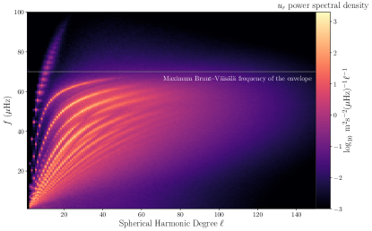
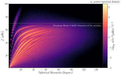
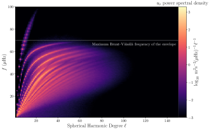
Figure 13: Spectral power density of $u_{r}$ at $19\mathrm{M}_{\odot}$ of M201 (top, 1000x heating, 0x diffusion), M204 (center, 1000x heating, 100x diffusion) and M207 (bottom, 1000x heating, 1000x diffusion).

The amount of radiative damping of the IGWs in the envelope is of interest when we consider the possibility that these IGWs cause material mixing in the envelope. The short wavelength waves that are damped substantially, as seen in Fig. 13, have no effect upon the asteroseismology observations of the waves at the stellar surface of massive stars, as they would be located in the region of white noise (Bowman et al., 2020). However, it is possible that the short wavelength waves have a significant impact on the efficiency of material mixing. This potential for IGW envelope mixing is explored at length in Paper I. Here we see that the short wavelength waves are damped by radiation diffusion. It is generally believed that radiative diffusion can play an essential role in IGW-induced mixing (e.g. Townsend (1958), Zahn (1974), Press (1981), Garaud et al. (2017), Paper I).

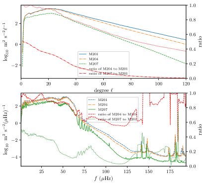
Figure 14: Power of radial velocity of M201, M204, M207, power ratio of M204 and M207 to M201 as functions of degree $l$ (Top: at 19 $M_{\odot}$) and as functions of frequency (Bottom).

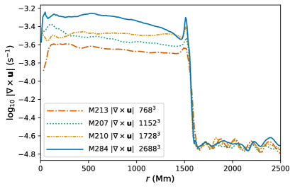
Figure 15: Vorticity of simulations with luminosity and radiative diffusion enhanced by 1000: M213 ($768^{3}$), M207 ($1152^{3}$), M210 ($1728^{3}$), M284 ($2688^{3}$). Although the vorticity increases with grid resolution inside the convection zone, it does not do so in the stably stratified envelope. This behavior has consequences for our ability to estimate gravity-wave-based mixing rates in the envelope using simulations with only modest grid resolution.

4 On the long-term evolution

The entrainment rate implied from linear growth of the entrained mass is too large to be compatible with the stellar model and observational properties (§3.3). Similar to the argument in section 3 of Paper I, if we assume that this entrainment rate applies for the entire $6.91\times 10^{6}$ $\mathrm{yr}$ main sequence lifetime of a 25 $\mathrm{M}_{\odot}$ star, a total entrainment of 630 $\mathrm{M}_{\odot}$  would be implied. This indicates that the entrainment we extrapolate cannot persist for even a fraction of the main sequence lifetime before the star goes through significant evolutionary changes. A motivation for the present work is to investigate whether or not including radiation pressure and radiative diffusion can result in entrainment that is more consistent with the main sequence stage of the stellar model. We have seen in §3 above that this additional physics causes the entrainment to decrease by only about $30\%$ . However, the linear growth of the entrained mass, the motion of the BV frequency peak, and the overshoot and undershoot of fluxes at the CB (Fig. 4) suggest that the simulated star is still in the process of thermal adjustment. Nevertheless, the velocity distribution in both the convective core and the radiative envelope has reached a dynamical equilibrium. We would like to establish whether or not continued entrainment and motion of the CB outward might alter the character of the flow in such a way that the entrainment rate might slowly diminish. This possibility is suggested by the recent work of Anders et al. (2022) investigating the long-term secular changes driven by thermal adjustment in a simplified Boussinesq, plane parallel, penetrative convection context.

Our explicit numerical technique in PPMstar requires us to explicitly follow sound wave signals in the low Mach number stellar flow. We have seen in Paper I and also here in Fig. 12 that we can overcome this limitation by appealing to empirically observed scaling laws. By enhancing the luminosity and the radiative diffusion by a common factor $X$, we speed up the evolution by a similar factor (actually slightly larger than $X$, as we will discuss later). In Paper I we saw that under these circumstances the velocities in the convection zone are enhanced by the factor $X^{1/3}$. If this enhancement of the velocities leaves them still at low Mach numbers, we do not expect the character of the flow to change significantly. As a rule of thumb, we might attempt to hold the resulting Mach numbers below 0.1, for which compressibility effects should be roughly of $1\%$ importance. A possible consideration is that we might raise velocities of wave motions in the stably stratified envelope to the level that makes the induced IGWs modes break. However, no wave breaking in the stable envelope shows up in the visualizations of any of our flows. To validate this technique for speeding up the evolution of our flows, we can generate a series of simulations at modest grid resolution that have different enhancement factors $X$ and that can be compared over at least an initial time interval of a reasonable length, long enough to go through a noticeable re-adjustment of thermal structure.

4.1 Key properties of the long-term evolution

We have performed such a series of simulations for the 25 $\mathrm{M}_{\odot}$ star which have enhancement factors $X$ = 1000, 3162, and 10000. These all have a grid resolution of $896^{3}$ cells, and all were run for relatively long periods of 507, 1189, and 1054 days for the star. For the case of largest $X$, this time duration is comparable to the thermal timescale of the simulated part of the 25 $\mathrm{M}_{\odot}$ star, namely $GM^{2}/2RL\approx 1000\mathrm{d}$, where $R=2500\ \mathrm{Mm}$ and $L=10000L_{*}$. This should be sufficient for the flow to relax to a state much closer to thermal equilibrium.

In the top panel of Fig. 16, we show the outward movement of the BV frequency peak. This peak marks the location within the radial entropy profile where the gradient is largest. This is also the location of the sudden jump in $f_{\rm V}$, the fractional volume of the stably stratified envelope gas. It is evident that the outward motion of the CB is continually slowing down as this simulation proceeds. The CB is still moving at the last time shown, but clearly it has slowed considerably.

Looking at Fig. 16, we notice that as the outward motion of the CB slows, there is an increasingly large region inside the CB (for time 17188 $\mathrm{h}$ between $r=1600$ and 1750 $\mathrm{Mm}$ where the BV frequency rises in the absence of any substantial contribution from the composition gradient. This feature of the later flow structures causes the convection to be reduced in intensity without causing additional entrainment. It would seem that this is a necessary feature for the entrainment rate to be diminished. The positive entropy gradient that is established in the growing penetration region between the SB and the CB, results from a balance between convective mixing of entropy which tends to reduce this gradient, and the small region of negative gradient of the radiative diffusion flux, shown in Fig. 17, which tends to build up the gradient. There is no corresponding mechanism to counteract the convective mixing of the composition, because the negative radiative diffusion flux gradient deposits entropy and has no effect upon the gas composition. Hence we see that $f_{\rm V}$ is efficiently mixed, even in the penetration region.

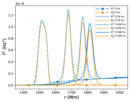
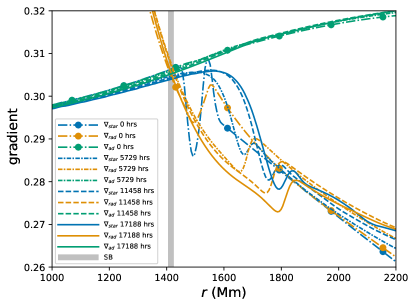
Figure 16: Top: $N^{2}$ and its compositional component (see Eq. 10) for dump 0, 2000, 4000, 6000. Bottom: radiative gradient, adiabatic gradient and actual temperature gradient for M252 (10000x) for the same dumps. The location of the SB is denoted by the thick vertical line around 1415 $\mathrm{Mm}$ which does not move much during the simulation. All profiles are computed from averages over 100 dumps.

In Fig. 16, the radiative gradient

$$\nabla_{\mathrm{rad}}\equiv 3\kappa LP/(16\pi acGmT^{4})\ ,$$

the actual gradient $\nabla_{\rm star}$, and adiabatic gradient $\nabla_{\mathrm{ad}}$ are plotted. The radiative gradient is defined as the gradient required so that all the luminosity is carried outward by radiative diffusion. The location, at roughly 1400 $\mathrm{Mm}$, of the SB, where $\nabla_{\mathrm{ad}}=\nabla_{\mathrm{rad}}$, does not change much during the course of the simulation. The actual gradient is strictly adiabatic inside the SB at $t=0$ by design via initialization. When the convection is fully developed, the actual gradient becomes slightly super-adiabatic inside 1000 $\mathrm{Mm}$ and slightly sub-adiabatic above 1000 $\mathrm{Mm}$ (Fig. 9) and gradually approaches the radiative gradient above the SB, as seen in Fig. 16. The outward motion of the CB noted earlier slows down, which is also shown by the change of the actual gradient with time. The penetration region, where the convective flux is negative above the SB, ends at 1850 $\mathrm{Mm}$  where the actual gradient starts to follow the radiative gradient, and the full luminosity is then carried outward by radiative diffusion alone (Fig. 17).

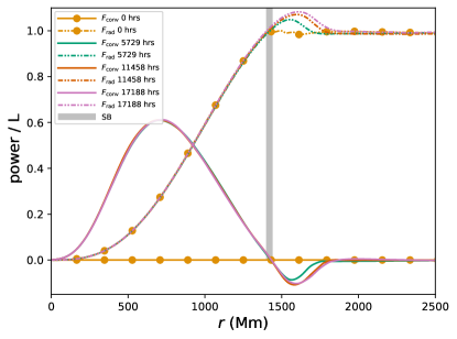
Figure 17: Radiative and convective energy fluxes (multiplied by $4\pi r^{2}$) for M252 (10000x) at dump 0, 2000, 4000, 6000, computed from averages over 100 dumps and 120 $\mathrm{Mm}$.

4.2 The governing equations

Similar to Anders et al. (2022); Roxburgh (1989); Arnett et al. (2015) (see also Korre & Featherstone (2021)), we attempt to model the convection zone by reducing the full set of hydrodynamic equations to 1D with reasonable assumptions. The governing hydrodynamics equations are the following:

$$\rho\frac{\partial\bm{u}}{\partial t}+\rho(\bm{u}\cdot\nabla)\bm{u} = -\nabla{p}+\rho\bm{g}{}$$ (14)

$$\frac{\partial\rho}{\partial t}+\nabla\cdot(\rho\bm{u}) = 0{}$$ (15)

$$T\frac{\partial}{\partial t}(\rho S)+T\nabla\cdot(\rho S\bm{u}) = \epsilon\rho-\nabla\cdot\bm{F}{}$$ (16)

where $S$ is the specific entropy, $\epsilon$ the rate of nuclear energy generation per unit mass, $\bm{F}$ the heat flux by radiative diffusion. These equations (Eq. 14 - Eq. 16) are equivalent to the Euler equations in conservation form solved by PPMstar. Taking the dot product of the equation for the conservation of momentum, Eq. 14, with the velocity results in the equation for kinetic energy

$$\frac{\partial}{\partial t}(\frac{1}{2}\rho u^{2})+\nabla\cdot(\frac{1}{2}\rho u^{2}\bm{u}) = -(\bm{u}\cdot\nabla)p+\rho\bm{u}\cdot\bm{g}\ .{}$$ (17)

Without any assumption so far, we integrate the kinetic energy density Eq. 16 over a thin spherical shell between radius $r$ and $r+dr$ and determine its rate of change in time,

$$\frac{\partial}{\partial t}\underset{(r,r+dr)}{\iiint}\frac{1}{2}\rho u^{2}dV= \underset{(r,r+dr)}{\iiint}(\rho\bm{u}\cdot\bm{g}-(\bm{u}\cdot\nabla)p)dV$$ (18)

$$-\underset{(r,r+dr)}{\iiint}\nabla\cdot(\frac{1}{2}\rho u^{2}\bm{u})dV{}$$

where the kinetic energy equation Eq. 16 is applied. We apply divergence theorem to the second term on the right-hand side and then approximate the resulting difference of surface integrals at $r$ and $r+dr$ with a differential, and finally approximate other volume integrals by surface integral multiplied by the shell thickness $dr$ to get

$$\frac{\partial}{\partial t}(\overline{\frac{1}{2}\rho u^{2}}4\pi r^{2}) =\overline{(\rho_{1}\bm{u}\cdot\bm{g}-(\bm{u}\cdot\nabla)p_{1})}4\pi r^{2}$$ (19)

$$\quad-\frac{\partial}{\partial r}(\overline{\frac{1}{2}\rho u^{2}u_{r}}4\pi r^{2})-4\pi r^{2}\overline{\Phi}{}$$

as $dr\to 0$, where $p=p_{0}+p_{1}$, $\rho=\rho_{0}+\rho_{1}$,$\nabla p_{0}=\rho_{0}\bm{g}$, subscript 0 denotes the initial hydrostatic state (or base state) quantities, subscripts 1 denote deviation from the initial hydrostatic state, $u_{r}$ is the radial velocity, $\Phi$ is the local dissipation rate of kinetic energy into heat, and the overbars $\overline{\cdot}$ represent averages over the $4\pi$ sphere at the radius $r$. Note that we assume that the viscosity does not enter directly, but only enters through the kinetic energy dissipation source term and entropy source term. We make this assumption because the viscosity of the stellar gas is one million times smaller than the thermal diffusivity $k/(\rho c_{p})$, $c_{p}$ is specific heat under constant pressure (the Prandtl number is $Pr\sim 10^{-6}$ for the stellar interior conditions considered here). Still, the viscosity is effective in dissipating the motions in the convection zone, while not dissipating motions elsewhere. The reason for this effectiveness of a truly tiny viscosity is that the convection zone is fully turbulent, and the turbulent cascade brings the motions there down to the tiny scales where the viscosity can act on them very efficiently to dissipate them into heat. We will discuss how to determine this dissipation rate in §4.3. Similarly,

$$\frac{\partial}{\partial t}(\overline{\rho S}4\pi r^{2}) =4\pi r^{2}\overline{\dfrac{\Phi}{T}}+\overline{\frac{1}{T}\nabla\cdot(\bm{\Gamma}-\bm{F})}4\pi r^{2}$$ (20)

$$\quad-\dfrac{\partial(\overline{\rho Su_{r}}4\pi r^{2})}{\partial r}{}$$

The nuclear energy generation is defined by the divergence of an energy flux by $\nabla\cdot\bm{\Gamma}=\epsilon\rho$ for convenience. Eq. 20 and Eq. 19 are the entropy equation and kinetic energy equation for each spherical shell.

4.3 Reduced equation for kinetic energy and turbulent kinetic energy dissipation

4.3.1 Reduced kinetic energy equation

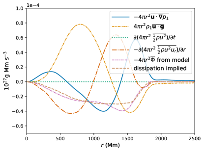
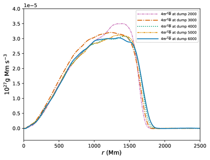
Figure 18: Top: work by pressure gradient and gravity field per unit time per unit radial distance, rate of change in kinetic energy per unit radial distance, radial derivative of total kinetic energy flux, dissipation derived from the turbulent dissipation model, measure dissipation rate per unit radial distance, averaged over 399 dumps centered at dump 6000 of M252; bottom: time sequence of measured turbulent kinetic energy dissipation of M252.

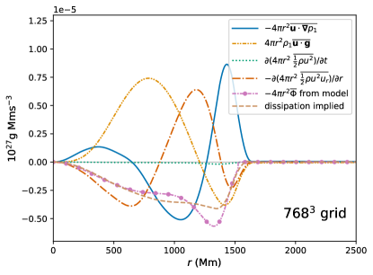
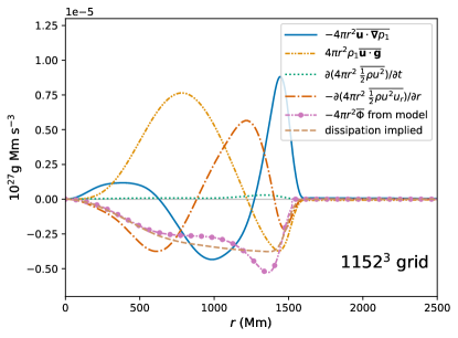
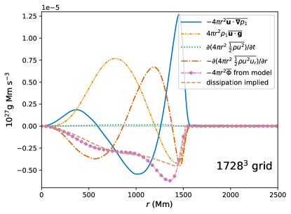
Figure 19: Work of pressure/gravity per unit time per unit radial distance, rate of change in kinetic energy per unit radial distance, radial derivative for the total kinetic energy flux, dissipation implied by the kinetic energy equation, dissipation from turbulence model for three resolutions of 1000x simulations (top to bottom: M213, M207, M210) for dump 2200 averaged over 401 dumps. Inside the SB at about 1400 $\mathrm{Mm}$ there is little dependence of these values on grid resolution. This means that we can get a good measurement of the implied turbulent kinetic energy dissipation rate using only a modest grid.

In our simulations, the gravity is static and determined by the base hydrostatic state. Therefore, the radial component of the base pressure gradient cancels out with the gravitational acceleration by design $\nabla p_{0}=\rho_{0}\bm{g}$. The gradient of the pressure perturbation, however, is not purely radial. Local high pressures can result in expansion in all directions. Hence, the pressure gradient term in the kinetic energy equation, which from the dot product evaluates to a scalar quantity, gives the work done by pressure per unit time per unit volume. The contribution of the horizontal components of the pressure gradient force $u\cdot\nabla p_{1}$ is not negligible, (Fig. 18). In particular, the peak in $u\cdot\nabla p_{1}$ near the CB comes mostly from the horizontal component of the pressure perturbation gradient. In this region rising gas hitting the CB causes local high pressure, and the resulting flows are turned horizontal with large $u_{h}\cdot\nabla_{h}p_{1}$. Thus the pressure gradient force term is significant even in low Mach number flows and cannot be found in a 1D computation except through a model, because of the 3D nature of convection.

The PPMstar code solves the inviscid compressible fluid dynamics equations, and physical viscosity is not included. This is reasonable, because the viscosity of stellar gas is truly miniscule. However, in the convective core the convection is turbulent. Turbulent dissipation of kinetic energy is important in the convection zone. This dissipation occurs via the turbulent cascade, which excites progressively smaller scales of motion until the viscous dissipation scale is finally reached. In our simulations, this dissipation is carried out by numerical truncation error terms, some of which act like viscosity, but with different dependence upon the spatial scale of the motion, see Porter & Woodward (1994). The effectiveness of numerical methods like PPM in simulating turbulent flows in this fashion has been discussed at length and in detail, with many examples, in Grinstein et al. (2007). There has been much work on modelling and theories for turbulent dissipation for stellar convection, for example, Zahn (1989), Porter et al. (1998), Woodward & Porter (2006), Arnett et al. (2008). From the averaged kinetic energy equation Eq. 19, the dissipation term can be deduced from the rest of the other terms,

$$\begin{split}-4\pi r^{2}\overline{\Phi}=&\frac{\partial}{\partial t}(\overline{\frac{1}{2}\rho u^{2}}4\pi r^{2})-\overline{(\rho_{1}\bm{u}\cdot\bm{g}-\bm{u}\cdot\nabla p_{1})}4\pi r^{2}\\ &+\frac{\partial}{\partial r}(\overline{\frac{1}{2}\rho u^{2}u_{r}}4\pi r^{2})\ .{}\end{split}$$ (21)

Woodward & Porter (2006) estimates the turbulent dissipation as a function of density, and turbulent kinetic energy density for homogeneous, isotropic turbulence,

$$\frac{\partial E_{\mathrm{turb}}}{\partial t}=-A_{0}\frac{1}{L_{0}}\sqrt{\frac{2}{\rho}}E_{\mathrm{turb}}^{3/2}{}$$ (22)

where $L_{0}$ is the integral length scale which is the scale containing most of the kinetic energy, a dimensionless parameter $A_{0}=0.51$, $E_{\mathrm{turb}}=\frac{1}{2}\rho u^{2}$, $u$ is the turbulent velocity. By inserting the spherical averages of density and velocity magnitude of M252 in Eq. 22 and using 1500 $\mathrm{Mm}$ here empirically as the spatial scale that contains most of the kinetic energy, we get an estimate of turbulent dissipation from the model.

Fig. 18 presents the the terms in the kinetic energy equation, including the dissipation rate implied by the simulation from assuming that all the measured terms plus this dissipation must add to zero, and it also shows the dissipation rate derived using the turbulence model. The core convection is not truly homogeneous, isotropic turbulence. However, its implied dissipation rate according to Eq. 21 agrees very well with the turbulent dissipation model. The same model for turbulent dissipation with a different factor has been reported in Frisch (1995) and Arnett et al. (2009). The agreement between the turbulent dissipation model Eq. 22 and the dissipation rate indirectly measured from the simulation is striking. Note that the turbulent dissipation model does not apply above the CB, where, by our definition of the CB, the net convective entropy flux becomes essentially zero and any motions are no longer turbulent. We therefore do not apply the turbulent dissipation model at the CB and beyond. The dissipation in the convection zone is a result of the turbulent cascade only. This is confirmed by the dissipation from the simulation decreasing smoothly to zero at around 1835 $\mathrm{Mm}$ in Fig. 18. The dissipation of kinetic energy implied by the simulation is negligible in the radiative envelope.

The numerical viscosity of the PPMstar method scales inversely with $\Delta x^{3}$, where $\Delta x$ is the cell width (Porter & Woodward, 1994). Each 1.5x grid refinement implies a decrease of numerical viscosity by a factor of 3.375. Hence, the results plotted in Fig. 19 show that the actual dissipation of kinetic energy is independent of the numerical viscosity, at least on a grid equal to or finer than $768^{3}$ for our simulation. As long as the convection is fully turbulent and there is an effective mechanism to dissipate kinetic energy on the smallest scales, we will end up with the statistically same dissipation rate.

4.3.2 Verification of turbulent dissipation measurement

Three simulations are performed, which restarted from a late dump (dynamical equilibrium already established) of the 1000x heating and 1000x radiative diffusion cases with 3 resolutions (M213, M207 and M210). Volume heating and radiative diffusion are turned off from the beginning of these three new runs. The intent is to measure the decay rate of the kinetic energy in the convective core, which should be the same as the turbulence dissipation rate. The kinetic energy per unit volume is plotted about every 8.5 hours in Fig. 20. Before the nuclear heating is removed, we have a slightly convectively unstable stratification. The unstable stratification continues driving the convection for a short while before it is eliminated. Hence, the decay of kinetic energy is barely noticeable in the first couple of dumps. The total decay rates of kinetic energy are estimated from the first 60 hours to be $20.5\%$, $17.8\%$ and $19.3\%$ (from low to high resolution) of the luminosity. Again, we do not see kinetic energy dissipated in the stable envelope.

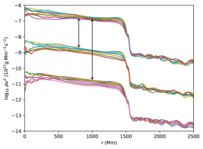
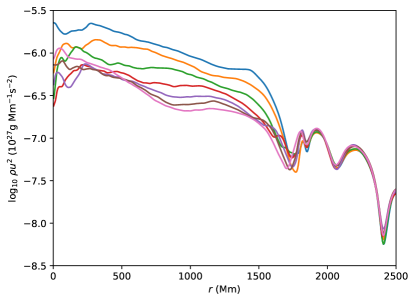
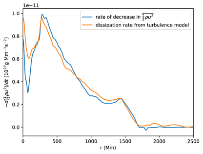
Figure 20: Top: time sequence of kinetic energy density every 8.5 hours for the rundown experiments of M210: $1728^{3}$, M207: $1152^{3}$ and M213: $768^{3}$ (upper, medium and lower groups of lines) where the medium and lower resolutions have been translated downward by 2 and 4, for easy visual comparison; Middle: time sequence of kinetic energy density every 8.5 hours for the rundown experiment of the M252: 10000x case; bottom: average decrease rate of kinetic energy from 20062 to 20082 hours measured from the rundown simulation of M252 and predicted by the model using the flow velocity at 20062 hours. Note that essentially no dissipation is seen outside the convection zone.

From the rundown experiment with the three resolution cases, we conclude that PPMstar converges on the behavior of the decaying kinetic energy in the context of no driving. Hence, again we see the dissipation rate is insensitive to the numerical viscosity. Because the initial slight super-adiabatic gradient converts gravitational potential energy to kinetic energy during the first few dumps, which acts as a source that affects the rate of change in kinetic energy, the change in kinetic energy is not caused by turbulent dissipation alone. In this respect convection differs from the case of uniform turbulence, where we can make a clean measurement of the dissipation just by stopping the stirring of the flow.

Similarly, we obtain the turbulent dissipation for a case with a higher luminosity enhancement factor by measuring the rate of change in kinetic energy directly from a simulation that begins from a late-time data dump of our long-time run M252. This 10000x heating simulation was restarted from 20062 hours with the volume heating and radiative diffusion turned off. The motion in the convective core dies down rapidly. The dissipation rate is measured from 20062 hours to 20082 hours assuming that it is constant in time at each radius. The decay rate of kinetic energy and the dissipation rate predicted by the turbulent model using 1500 $\mathrm{Mm}$ as $L_{0}$ are shown in Fig. 20. Because we have started this run-down experiment from a very late time, we get an indication in Fig. 20 of the behavior of the dissipation rate in the penetration region beyond the SB when the flow is close to thermal and dynamical equilibrium.

4.3.3 Reduced entropy equation

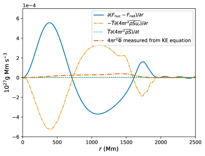
Figure 21: The gradient of energy flux from nuclear heating and radiative diffusion, gradient of the advective entropy flux multiplied by temperature, rate of change in entropy multiplied by temperature, dissipation of kinetic energy measured at dump 6000 of run M252. Note the small role played by turbulent kinetic energy dissipation relative to the other terms in the entropy equation.

Now we proceed to investigate the reduced entropy equation to see if it leads to useful 1D modelling that has predictive power on whether the star is in equilibrium or how big the convective penetration region should be. There is no approximation in deriving Eq. 20. The entropy equation simply states that the rate of change of entropy in a spherical shell is the sum of turbulent dissipation of kinetic energy, heating and cooling of nuclear burning and radiative diffusion, and the advective flux of entropy. To further simplify, we assume the divergence of the radiative diffusion is mostly radial, which is not strictly true because the adiabatic motion will heat or cool fluid parcels, and then the heat flux can have a non-zero horizontal component. The second term on the right-hand side then becomes

$$\overline{\frac{1}{T}\frac{\partial(\Gamma_{r}-F_{r})4\pi r^{2}}{\partial r}}\equiv\overline{\frac{1}{T}\frac{\partial(F_{\mathrm{nuc}}-F_{\mathrm{rad}})}{\partial r}}.$$

The advective entropy flux mostly cancels with the nuclear heating plus the radiative flux, leading to a negligible time rate of change in the entropy (see Fig. 21). The dissipation per unit radial distance is small compared to the derivative of advective entropy flux multiplied by the temperature and to the $\partial(F_{\mathrm{rad}}-F_{\mathrm{nuc}})/\partial r$ term, but not small compared to the measured time rate of change in the entropy. Of course, for a simulation in perfect equilibrium the latter would be zero.

As was pointed out in §3.2.4, the superadiabaticity changes its sign at 1000 $\mathrm{Mm}$. Beyond that location, the stratification is slightly convectively stable, but there is still convection. The convective motions are not significantly damped by the tiny amount of subadiabaticity between 1000 $\mathrm{Mm}$ and the CB until the gas is subjected to a significant stabilizing force in the penetration region beyond the SB. The time rate of change in kinetic energy and entropy is very small compared to the source terms and the flux terms. This by no means implies, however, that the star is in thermal equilibrium, because small changes over long times are seen in our long duration run M252 to have significant effects.

4.3.4 Accelerating stellar evolution by enhancing luminosity and radiative diffusion

In the work reported in Paper I and in earlier work, we have applied luminosity enhancement to increase the fluid velocity. The convective velocity is greater with luminosity enhancement (Fig. 7). We then extrapolate the entrainment rate to nominal heating using the scaling relation we observe in a series of runs with different luminosity enhancements. Enhancing the radiative diffusion accelerates the thermodynamical evolution. Hence, enhancing both the luminosity and diffusion by the same multiplicative factor accelerates both convection and thermal adjustment.

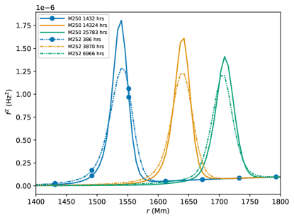
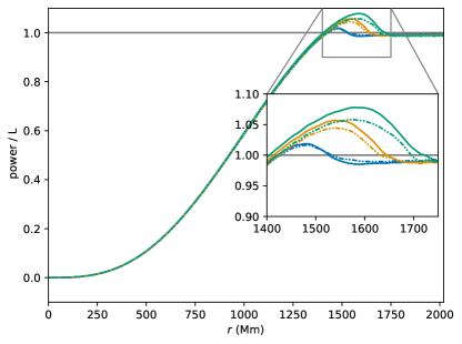
Figure 22: $N^{2}$ of M250 (3162x) and M252 (10000x) at three different times when they proceed to the same location; Bottom: total radiative heat flux of M252 (10000x) and M250 (3162x). Considering that $N^{2}$ depends upon the local entropy gradient, it is remarkable how similar the results of these two runs are at these times, especially considering the more than 3 times greater computational cost of the M250 results.

Comparing the vertical scales of Fig. 19 and Fig. 18 suggests that the terms in the kinetic energy equation scale linearly with the boosting factor. The scaling of convective velocity with luminosity (Fig. 7) and the turbulent dissipation model Eq. 22 also imply that the turbulent dissipation scales linearly with the luminosity enhancement. Hence, the turbulent dissipation, $\bm{F}$, and $\bm{\Gamma}$ in Eq. 20, all scale linearly with the boosting factor $L/L_{*}$. The time rate of change in entropy is driven to become very small on the thermal timescale if the star is nearly thermally relaxed. Then the entropy flux has to scale with the boosting factor, as the rest of the terms in the entropy equation do so, and their sum, the time rate of change of entropy, is nearly vanishing. This behavior is also demonstrated by the simulation, as can be seen in Fig. 21. Hence, the rates of change with time of kinetic energy and entropy are small when the stratification is close to equilibrium, and this implies that the rest of the terms in the kinetic energy and entropy equations must scale with the enhancement factor. Naturally, we would hope the rate of change with time also scales linearly with the enhancement factor, so that we can reasonably accelerate our simulations by boosting luminosity and thermal conductivity by the same factor.

From the perspective of simulation, we present evidence here that stellar thermal evolution can be accelerated by enhancing the luminosity and the radiative diffusion by the same factor. The accelerated evolution is meaningful only if the simulation arrives at a similar stratification within a shorter time. We see in the bottom panel of Fig. 22, the convective and radiative fluxes of the two higher luminosity runs plotted at times inversely proportional to their enhancement factors $X$. These fluxes agree very closely, which is consistent with our intent that we can speed up the flow evolution by enhancing luminosity. Fig. 22 demonstrates that boosting the luminosity by a factor of 3.162 accelerates the evolution by a factor of about 3.6, after eating away the initial CB profile and later establishing a similar profile as a spherical average of a dynamic 3D flow. The rate of thermal relaxation, with the mixing as one of the processes, does not necessarily scale precisely with the luminosity. This can be observed by comparing entrainment rates for M207 and M209 at 1000x and 3162x enhancement (Table 1). The ratio of their entrainment rates is $1.36\mathrm{M}_{\odot}\ \mathrm{yr}^{-1}/0.369\mathrm{M}_{\odot}\ \mathrm{yr}^{-1}\sim 3.69$.

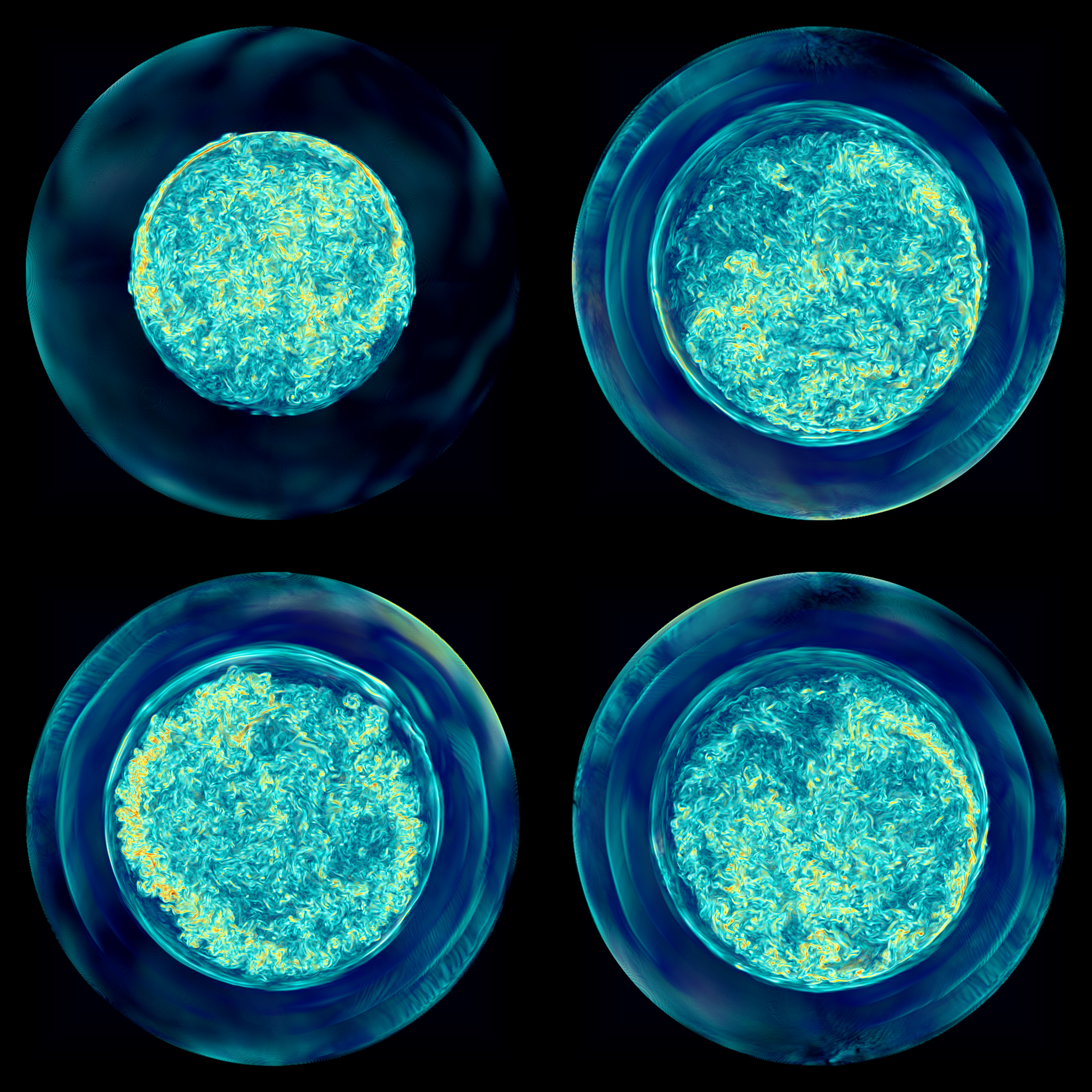
Figure 23: Four views of the vorticity magnitude in the far hemisphere of a non-rotating main-sequence stellar model of 25 solar masses are shown (M252, 10000x $L_{*}$ & $K_{*}$). The simulation was computed on a grid of $896^{3}$ cells, and in this simulation the luminosity of the star was boosted by a factor of 10000 in order to speed its approach to a dynamical and thermal equilibrium state. The image at the top left shows the star at time 12.06 days, when the dipole circulation pattern characteristic of core convection has become well established. The other three views of this same stellar model are shown at a much later time, when the flow has developed a much larger region of penetrative convection above the SB. Going clockwise from the top-right, these three later views are at times 732.41, 732.76, and 737.66 days. In the early flow, we see that the classic core-convection dipole circulation hugs the CB closely over about a quarter of the extent of this circle. The flow separates from the CB where the prominent shear layers, marked by very strong vorticity (shaded yellow), bend inward from the boundary. At top right, we see the flow much, much later. The convection zone has expanded substantially, and the dipole circulation ”contacts” the CB only along a very small segment, from which it immediately separates. Just 0.35 days later, at bottom right, the dipole circulation has left the CB entirely, leaving a thin layer of somewhat higher entropy gas between it and the boundary. In the image at the bottom left, despite the vigor of the dipole circulation flow, we see no contact with the CB, but we do see at about 2 o’clock, a strong gravity wave interfacial mode propagating along the CB, with a node in its flow pattern right at the CB radius. Our model of the convection zone identifies the thin, higher-entropy layer of convection zone gas right next to the CB as a key feature of this near-equilibrium penetrative convection structure. This layer is generated by local heating from a declining radiative diffusion heat flux that is approaching the total luminosity in this region from above. Our analysis indicates that the size of the convection zone, the location of the SB, and the structure of the penetration region does not change with the luminosity boost factor.

.

We have shown in Fig. 16 that the outward motion of the convective boundary, as indicated by the BV frequency peak location, slows greatly at late times in our run M252 with the luminosity and radiative heat conduction both boosted by a factor of 10,000. We have also argued that the simulation data suggest that the slowing of this outward motion occurs as a result of the development of a thin region just inside the compositional jump at the boundary in which there is a positive entropy gradient without any significant compositional change. This entropy gradient is maintained despite convective mixing by the local heat deposition caused by the negative radial gradient of the radiative heat flux as it approaches the full stellar luminosity value from above. The volume-rendered vorticity images in Fig. 23 give us a sense of how the convection flow changes as it approaches equilibrium. At early times, as seen in the image at top left, the dipole circulation pattern has the upwelling flow strike the composition jump at the convective boundary, become deflected, and travel along the boundary for a considerable distance. The snapshots in Fig. 23 cannot convey it, but indeed at early times the dipole circulation maintains its orientation and flows along the convective boundary for significant amounts of time before this orientation changes and the upwelling strikes the boundary in a different location. The dipole direction wanders constantly, but at early times there is a continual transport of gas from above the convective boundary, with this gas collecting at the location where the opposing flows along the boundary meet and plunge back toward the center of the star (about 5 o’clock in the top-left image in Fig. 23). At the much later times shown in the three later images in Fig. 23, the dipole circulation pattern is changing its direction more rapidly, and it is causing the upwelling gas to actually meet the compositional change at the convective boundary only briefly and occasionally. This means that the convection flow is far less effective at these late times in bringing stably stratified gas into the convection zone. In fact, the flow at this time is much more like the standard picture of rising plumes overshooting or penetrating into a stably stratified region. In this core convection flow, we have mainly a single ”plume” provided by the dominant dipole circulation, but it does appear to overshoot from time to time and at constantly varying locations along the convective boundary. This feature of the core convection flow suggests that for a convective shell, where the largest significant eddies are not global in scale, we might well expect the same forces working on the flow as it approaches equilibrium to produce the phenomenon of occasional identifiable plumes overshooting into a region of a stable entropy gradient, as has been observed in the simulations of Baraffe et al. (2017); Pratt et al. (2017, 2020); Korre & Featherstone (2021).

5 How to find a convection zone with penetration in equilibrium

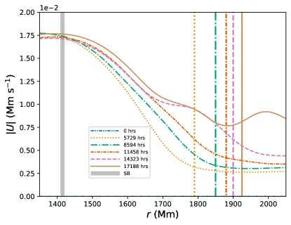
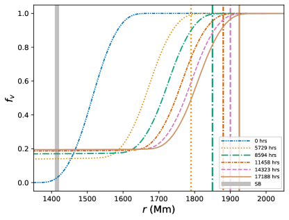
Figure 24: Spherical average of convective velocity and $f_{\rm V}$, averaged over 200 dumps, and over 20 radial points (equivalent to 116 $\mathrm{Mm}$) twice, of M252 (10000x $L_{*}$ & $K_{*}$) at dump 0, 2000, 3000, 4000, 5000, 6000. The location of the SB is denoted by the thick vertical line around 1415 Mm which does not move much during the simulation. The CB for all dumps except dump 0 are vertical lines at 1780 $\mathrm{Mm}$, 1850 $\mathrm{Mm}$, 1880 $\mathrm{Mm}$, 1900 $\mathrm{Mm}$, 1910 $\mathrm{Mm}$. The CBs are identified by the locations where the total convective entropy flux levels off, see Fig. 25.

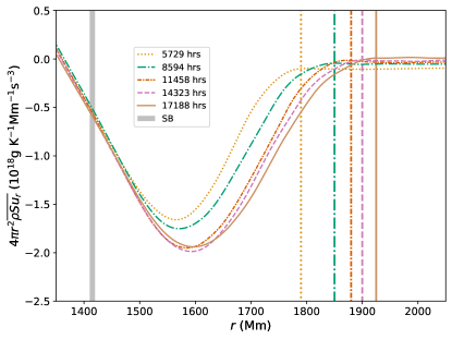
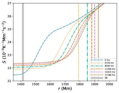
Figure 25: For run M252, spherical average of total entropy flux averaged over 200 dumps, and of entropy per unit mass, averaged over 200 dumps, and over 20 radial points twice, at dump 2000, 3000, 4000, 5000, 6000.

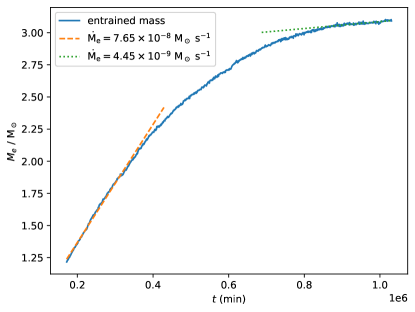
Figure 26: Entrained mass as a function of time of M252. Over the course of this long simulation, the entrainment rate has dropped by about a factor of $\sim 17$, although it has not fallen to zero when the simulation was stopped. The entrainment rates are measured from dump 1000 to 2000, and from dump 5000 to 6000 (durations of 278 $\mathrm{h}$)

The jumps in $f_{\rm V}$, $|U|$ are shown in the panels of Fig. 24, and Fig. 25 shows entropy advective flux and entropy profiles, with the CB location indicated by the location of vanishing flux. We see that at the CB, the fluid motions essentially stop, even though they do change character as we approach the CB within the thin region of the sharp entropy jump, as has been noted in Paper I. In Fig. 25, we show data from run M252, our case with $X=10000$. Even at the last time shown, the CB is still moving outward, but it has clearly slowed considerably.

From §4 discussing the simulation on the thermal timescale, we find that (1) penetrative convection develops above the SB (Fig. 25), (2) the entrainment decreases significantly at later times as the penetration region develops (Fig. 25 and Fig. 26), (3) there is a positive entropy gradient that develops in the penetration region (Fig. 25), (4) the convection is slowed down by the positive entropy gradient before it reaches the compositional gradient, which suppresses the entrainment significantly. We note that the $f_{\rm V}$ jump acts as a relatively hard barrier to the convection flow at every stage of the enlargement of the penetration zone, and it is undeniably dynamically important. It continues to move outward until the return of the overshooting radiation diffusion heat flux to the full luminosity is able to heat the gas in the penetration zone sufficiently to nearly arrest its outward motion. In the near equilibria shown in Fig. 27 it is clear from the curves plotted for the convective entropy flux that very little convective transport is still happening at the latest times shown in the range of radii in which $f_{\rm V}$ increases rapidly. All these observational properties suggest that our model star is approaching equilibrium asymptotically. A natural question to ask is whether or not we can find the ultimate equilibrium state, a convective core with penetrative convection in thermal equilibrium, that our simulation is approaching. At present, we are prevented from doing this by simply running our simulation further in time. However, we would like to explore the question of whether we can predict what the final equilibrium state is likely to be.

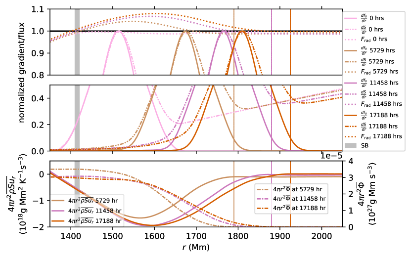
Figure 27: Top and middle: convective/radiative energy flux with $f_{\rm V}$ and entropy gradient normalized to 1 at dump 0, 2000, 4000, 6000 (0, 5729, 11458, 17188 $\mathrm{h}$). Bottom: total entropy flux and the measured dissipation rate per unit radial distance. All are averaged over 200 dumps, and over 20 radial points twice except for dump 0.

5.1 Roxburgh criterion

The evolution of our run M252, with $X=10000$, shows us that the convection flow, given sufficient time, develops a significant penetration region beyond the SB. In this region the total radiative flux exceeds the total nuclear heating rate, and this excess is compensated for by a negative convective flux. For carrying out 1-D stellar evolution simulations, we would like to have a model of convection that includes such a penetration region and that relates its extent to other parameters of the problem. Anders et al. (2022) addressed this problem by relating their simplified convection model to the arguments made by Roxburgh (1989). Roxburgh (1992, 1989) developed a constraint that a convection zone in an equilibrium state should satisfy. This constraint, known as the Roxburgh criterion,

$$\int_{0}^{r_{c}}(F_{\mathrm{rad}}-F_{\mathrm{nuc}})\frac{1}{T^{2}}\frac{dT}{dr}dr=0{}$$ (23)

where $F_{\mathrm{rad}}(r)$ is the total radiative energy flux, $F_{\mathrm{nuc}}(r)$ is the total nuclear energy flux at radius $r$, is an equation of the volume integral over the convective core bounded by the CB, at radius $r_{c}$, derived from the time evolution equation for the entropy. In brief, the entropy equation is integrated over the spatial extent of the convection zone, which in our case is from the center of the star out to the CB. Roxburgh assumed that the vector velocity vanishes everywhere on the spherical surface that we call the CB. Roxburgh assumes time-stationary convection, and of course our continued, although small, entrainment invalidates this assumption. Nevertheless, it is possible that the Roxburgh constraint Eq. 23 is nearly satisfied for our runs.

We examine the integral of the entropy equation without the assumption of being dissipationless (Eq. 24), by inserting the radial profiles of temperature, entropy, measured turbulent dissipation rate (by subtracting the sum of all other terms in the kinetic energy equation from zero) and radiative flux of M252,

$$\int_{0}^{r_{c}}(F_{\mathrm{rad}}-F_{\mathrm{nuc}})\frac{1}{T^{2}}\frac{dT}{dr}dr=\int_{V}\frac{\Phi}{T}dV{}$$ (24)

where $\Phi$ is the turbulent dissipation rate. The development of penetration and the resulting extended region of turbulence indicate that the convection is driven towards equilibrium but is not there yet (see the equality/inequality of the Eq. 24 with Table 2). Nevertheless, illuminated by the evolutionary trends of M252, we can devise a means of producing the final equilibrium state for this particular star, which we set out in §5.3.

Table 2: Numerical values of Roxburgh integral derived from spherical averages, and temperature weighted integral of dissipation measured from kinetic energy equation of run M252. Both are in units of $10^{18}~{}\rm{g\ \mathrm{Mm}^{2}s^{-3}K^{-1})}$.

Dump	$\int_{0}^{r_{c}}(F_{\mathrm{rad}}-F_{\mathrm{nuc}})\frac{1}{T^{2}}\frac{dT}{dr}dr$	$\int_{V}\frac{\Phi}{T}dV$	$r_{f_{\rm V}=0.5}/\mathrm{Mm}$
2000	0.280	0.225	1800
4000	0.258	0.216	1872
6000	0.242	0.213	1950

5.2 Entropy flux

We hope to devise a method to find the equilibrium convection zone structure that can be used in conjunction with 1D stellar evolution codes. Because $u\cdot\nabla p_{1}$ is inherently 3D by nature, we choose to work with the entropy equation, reducing it to 1D with assumptions that might be only minimally violated in 3D. Our simulations are initialized from the 1D stratification specified by MESA. The 1D MESA model is in hydrostatic and thermal equilibrium, because the nuclear timescale is much greater than either the thermal timescale or the dynamical timescale. By assuming a time-stationary state and spherical symmetry, because we are interested in the ultimate equlibrium state, and ignoring non-radial radiative heat flux, the entropy equation for every spherical shell becomes

$$\frac{\partial(\overline{\rho Su_{r}}r^{2})}{\partial r}4\pi=\overline{\frac{\Phi}{T}}4\pi r^{2}+\overline{\frac{1}{T}\frac{\partial(F_{\mathrm{nuc}}-F_{\mathrm{rad}})}{\partial r}}.{}$$ (25)

In this equation we use the assumption of a steady state with zero time derivative to enable us to solve for the convective flux term on the left. This term would be quite difficult to obtain through modeling, using mixing length arguments, but the terms on the right in this equation, at least the second such term, are easy to pin down in a 1-D computation. The nuclear heating input and the radial temperature and opacity structure come directly out of a 1-D simulation. The kinetic energy dissipation rate, which appears here as a heat source, does not. However, we have seen that we can solve for it using the kinetic energy equation in a similar fashion, as we will explain below.

5.3 A procedure to compute the extent of the penetration zone

In discussing the long-time behavior of our simulations of core convection, we found it notable that as the convective penetration region beyond the SB very slowly was extended outward, with the accompanying ingestion of stably stratified gas from the radiative envelope, the structure of the convection flow inside the SB radius changed hardly at all. This can be seen in Fig. 17 and Fig. 18. It is reasonable that this should be the case, because the region of convective penetration is not so very large in comparison to the convection zone as a whole. The extent to which the structure inside the SB does not change over the course of our long 3-D run M252 can also be assessed by examining the plots in Fig. 24 and Fig. 25. In these plots, the radii shown begin just inside of the SB, but it is nevertheless clear that for all the times shown the behavior near the SB is very closely the same. This insensitivity of the flow structure inside the SB to the development of the convection structure outside of it allows us to pin down the kinetic energy dissipation rate, shown in Fig. 18, inside the SB in a practical manner.

We determine the unknown dissipation rate, $\Phi(r)$, by performing a short-duration 3-D convection simulation on a modest grid. From the data shown in Fig. 19, we see that, at least with PPMstar, a grid of $768^{3}$ cells is sufficient. We begin with the 1-D structure produced by a stellar evolution code, use it to initialize our 3-D grid, and then run the simulation through its initial transient adjustment to 3 dimensions. After producing enough data to give us good time averages over multiple large eddy turn-over times, we can stop the run and measure the time-averaged radial profiles of the terms in the kinetic energy equation, which are shown in Fig. 19. If we have carried the run far enough in time, we will be able to verify that the time average of kinetic energy at each radius is nearly zero, as can be seen in Fig. 19. We can then use this vanishing of time derivatives to solve for the kinetic energy dissipation rate, $\Phi(r)$, using equation Eq. 21. This procedure allows us to build a first-principles model of the convection zone with its penetration region without involving paramters that would need to be calibrated against observations.

One might think that pinning down our 1-D model of the convection zone by solving a 3-D flow problem invalidates the advantage of a 1-D model. This might be true if we had to perform 3-D simulations often in order to carry a stellar model from the zero-age main sequence through its lifetime as a star. But this is unlikely to be the case. We can parameterize $\Phi(r)$ and match that form to the measured result from a 3D simulation only at wide intervals in time during the star’s evolution. A very simple model would relate $\Phi(r)$ to $|u(r)|$ through the turbulence model formula, Eq. 22, get $|u(r)|$ from the standard MLT estimate taken at a radius well inside the SB, and apply that value everywhere inside the SB. Fitting this to the 3-D simulation results would involve some constant of order unity, which could be checked and rechecked at regular time intervals against new 3-D simulations. On modern computing equipment, 1-D stellar evolution simulations cost very little, so that adding to that cost a few modest 3-D simulations should not be a problem. In any case, a table of results could in principle be generated and made available over the Internet.

With the convection flow pinned down inside the radius of the SB, our challenge remains to extend it outward to the CB. To do this, we can be guided by the long-time behavior that we have described in the previous section. In Fig. 24 and Fig. 25 we see how the convection flow slowly develops as it approaches an equilibrium structure. First, Fig. 18 shows how $\Phi(r)$ changes during this process. Its value at the SB stays roughly constant in time, while its value at the CB is, of course, zero. In addition, we can see that demanding that ${\partial\Phi}/{\partial r}$ vanish both at the SB and at the CB is a very reasonable constraint. We may then approximate $\Phi(r)$ between the SB and CB as a cubic polynomial, in which case it is uniquely determined. To get this function to approach zero more gradually, we could additionally demand that its second radial derivative vanishes at the CB. Then we would need to make this function a quartic polynomial. In this region, $\Phi(r)$ will be small relative to other terms, but it will nevertheless play an important role, because it is never negative.

The terms of the entropy equation are plotted in Fig. 21. In the absence of a long-duration 3-D simulation, it would be very hard to guess the functional form of $-4\pi T{\partial(r^{2}\rho Su_{r})}/{\partial r}$, which is plotted in Fig. 21. However, we know that in the absence of a time derivative of $\rho S$, this gradient of the convective entropy flux must cancel the sum of $\Phi$ and the gradient of the radiative heat conduction flux (Eq. 25). We have a model for $\Phi$, and if we can provide a model for ${\partial(F_{\rm nuc}-F_{\rm rad})}/{\partial r}$, then we can simply solve for the convective entropy flux using Eq. 25.

We know the value of $F_{\rm rad}$ and its first 2 derivatives at the SB, and we know that $F_{\rm rad}$ must equal $L$, by definition, at the CB. Looking at the results of our simulation shown in Fig. 25, it seems reasonable to assume that the first two radial derivatives of $F_{\rm rad}$ vanish at the CB. If we demand that $F_{\rm rad}$ be a quintic polynomial between the SB and the CB, these 6 constraints determine it uniquely. This determination then is enough to allow us to solve for the convective entropy flux term, $-4\pi T{\partial(\overline{r^{2}\rho Su_{r}})}/{\partial r}$, between the SB and CB. Of course, to do this, we must first guess a location for the CB. We cannot just make any guess for the CB location. Our model assumptions are sufficient to determine the terms in the entropy equation, Eq. 20, in its steady-state equilibrium form, which is Eq. 25. We need one further condition in order to distinguish the CB radius from all the possible guesses for it that we might make.

The final constraint that we need to impose in order to fully determine our 1-D model of the full convection zone is the demand that the convective entropy flux at the CB must vanish. To check whether this constraint is satisfied for any particular choice of the CB location, we can begin at the central fluid state at $r=0$ that we get from the 1-D stellar evolution code, and we can integrate outward in radius along an adiabat to the SB, remaining in hydrostatic equilibrium at each step. In this process, we keep the composition, $f_{\rm V}$, constant, because the convection zone is well mixed inside the SB. At each radius, the isentropic, hydrostatic fluid state determines both $F_{\rm nuc}$ and $F_{\rm rad}$. Because we know $\Phi(r)$, as described above, we may solve for $-4\pi T{\partial(\overline{r^{2}\rho Su_{r}})}/{\partial r}$. This convective entropy flux gradient allows us to determine the flux itself, $\overline{\rho Su_{r}}$, at our radius, if we have produced it at the previous radial step outward. In this process, we can determine the full fluid state and also the flux $\overline{\rho Su_{r}}$ at the SB

The conditions of our model, as just described above, are sufficient to carry this integration process onward to the CB if (1) we know the CB location and (2) we know $f_{\rm V}(r)$ between the SB and the CB. We know that $f_{\rm V}$ cannot be constant in this region, because it must be unity at the CB. Efficient convective mixing keeps $f_{\rm V}$ at a constant value below unity inside the SB, but inside the penetration region this mixing efficiency must be diminished progressively as the CB is approached. We appeal to the results of our 3-D simulation shown in Fig. 24 and Fig. 25 to produce a model for $f_{\rm V}(r)$. We focus particularly on the later times shown in that figure. It is clear that the sudden, but still smooth jump in $f_{\rm V}$ comes right at the end of the penetration region, and this jump is complete at the CB. It is also clear that there is a substantial smooth rise in entropy, S, immediately before the jump in $f_{\rm V}$ begins. That rise in entropy is caused by local heating due to the return of the radiation heat conduction flux, $F_{\rm rad}$, to the full luminosity value, $L$. We will assume, and it is of course an assumption rather than an established fact, that the jump in $f_{\rm V}$ begins at the point where this local heating rate has its maximum, hence where ${\partial^{2}F_{\rm rad}}/{\partial r^{2}}$ vanishes and also ${\partial F_{\rm rad}}/{\partial r}$ is negative. Between this point, which we call $r_{\rm foot}$, and the CB, at $r_{\rm CB}$, we assert that the shape of $f_{\rm V}(r)$ is that of the sine wave between values of its argument of $-{\pi}/{2}$ and ${\pi}/{2}$. Thus, we have the expression for $f_{\rm V}(r)$ as

$$f_{\rm V}(r)= \frac{1}{2}[1+\sin(\pi\frac{r-r_{\rm foot}}{r_{\rm CB}-r_{\rm foot}}-\frac{\pi}{2})](1-f_{\rm V}(r_{\rm SB}))$$ (26)

$$+f_{\rm V}(r_{\rm SB}){}$$

where $r_{\rm foot}<r<r_{\rm CB}$. Now it is possible to use a Newton iteration over the CB radius $r_{\rm CB}$ to converge upon a model of the convection zone including its penetration region, and that model will satisfy the following assumptions and constraints:

• The central state of the gas is given by the central state produced by the 1-D stellar evolution code, with a composition, $f_{\rm V}$, that reflects any additional entrained material from above the CB.

• The state of the gas inside the SB has the same entropy and composition as the state at the center, and it is in hydrostatic equilibrium.

• The kinetic energy dissipation rate, $\Phi(r)$, inside the SB is determined from a short-duration, modest grid, 3-D simulation that has achieved dynamical equilibrium, in that the time derivative of the kinetic energy everywhere inside the SB essentially vanishes.

• Inside the SB, where by definition $F_{\mathrm{rad}}=L$, both $F_{\mathrm{nuc}}$ and $F_{\mathrm{rad}}$ are determined by the fluid state.

• Inside the SB, the convective entropy flux, $4\pi r^{2}\overline{\rho Su_{r}}$, satisfies Eq. 25.

• Between the SB and the CB, $\Phi(r)$ is the unique quartic polynomial continuous at the SB with vanishing radial derivative there and vanishing at the CB, with vanishing first two radial derivatives there.

• Between the SB and the CB, $F_{\rm rad}(r)$ is the unique quintic polynomial that is continuous and twice continuously differentiable at the SB and which equals $L$ with vanishing first two radial derivatives at the CB.

• Between the SB and the CB, $F_{\rm rad}(r)$ has its minimum (negative) radial derivative at $r=r_{\rm foot}$.

• Between $r_{\rm foot}$ and the CB, the composition, $f_{\rm V}$, rises smoothly from its constant value inside $r_{\rm foot}$ to unity at the CB with the shape of a sine wave between its argument values of $-\pi/2$ and $\pi/2$, see Eq. 26.

• Between the SB and the CB, the convective entropy flux, $4\pi r^{2}\overline{\rho Su_{r}}$, satisfies Eq. 25, and it vanishes at the CB.

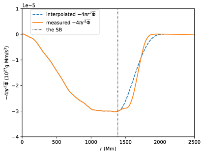
Figure 28: Top: dissipation measured from M252 at dump 6000 and interpolated beyond the SB; bottom: entropy flux implied by the predicted hydrostatic equilibrium stratification using the measured dissipation inside the SB and the interpolated dissipation above the SB. The 1st prediction uses central density, entropy and $f_{\rm V}$ and turbulent dissipation below the SB at dump 2000, 2nd at dump 4000, 3rd at dump 6000.

When stepping outward from the SB to the CB, we replace the isentropic condition we used to arrive at the SB with the demand that a hydrostatic fluid state must also have the prescribed radiative heat conduction flux. We have found such model solutions, starting from the state given by our M252 long-duration run at the three times shown in Fig. 24, and these model convection zone equilibrium structures are shown in Fig. 28. In Fig. 30 (top panel), we show the three model convection zone equilibrium structures that we arrive at starting with states in our three runs, M250, M251, and M252, when their peak values of ${\partial f_{\rm V}}/{\partial r}$ are all located at nearly the same radius. These three runs have luminosity enhancement factors of 1000, 3162, and 10000, and we compare their implied equilibria at times 716, 202, 48 days. We see that the implied equilibria are very nearly identical, which supports our discussion of the linear scaling with luminosity enhancement factor of the terms in the kinetic energy and entropy equations. For the three implied equilibria to agree, we must also have the width and location of the compositional jump in $f_{\rm V}$ agree. That this agreement between the $f_{\rm V}$ profiles is very nearly observed in the simulation results at these times is shown in Fig. 30 (bottom panel). We note that in Fig. 30 the $f_{\rm V}$ values used come from radial profiles in which we have performed no time averages or moving spatial averages that could broaden the compositional jumps so that they become more similar. The closely matched width and shape of the $f_{\rm V}$ jumps in these three runs with luminosity boosts ranging over a factor of 10 is remarkable. The rise in $f_{\rm V}$ from 0.1 to 0.9 in these radial profiles takes 6 to 7 grid cell widths. Our PPB moment-conserving advection scheme in PPMstar is able to describe and maintain sharper rises than this, but it is nevertheless possible that this 6-cell width represents a minimum that is produced by the combination of the PPB scheme and our method for producing a radial profile from data on our Cartesian grid. That such a doubt exists underscores the fact that the composition jump right inside the CB in our simulations and in our model is a thin feature, and therefore if the model does misrepresent its thickness, it cannot do so by very much. We also note that although one might imagine that this entire procedure could be simplified by approximating the kinetic energy dissipation rate with zero everywhere, we find that doing this makes it impossible to find a solution satisfying all these simultaneous constraints.

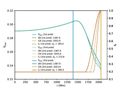
Figure 29: Actual temperature gradient (Eq. 10) implied by the predicted hydrostatic equilibrium stratification using the measured dissipation inside the SB at dump 6000 and the interpolated dissipation above. The $f_{\rm V}$ transition starts from 185 $\mathrm{Mm}$ (1st), 275 $\mathrm{Mm}$ (2nd, used in the procedure of this work) and 385 $\mathrm{Mm}$ (3rd), where the middle one is the location of the smallest derivative of $F_{\mathrm{rad}}$ in the penetration zone.

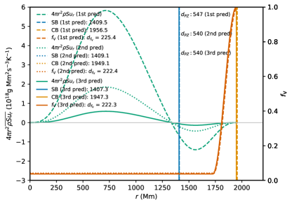
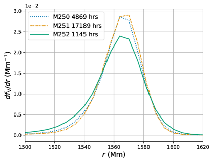
Figure 30: Entropy flux (top) implied by the predicted hydrostatic equilibrium stratification using the measured dissipation inside the SB and the interpolated dissipation above the SB at three times corresponding to dumps 400, 1700, 6000 when $f_{\rm V}$ gradient peaks (bottom) are located at about the same location for M252 (1st, 10000x), M250 (2nd, 3162x), M251 (3rd, 1000x). These entropy flux curves are all the same to within 1.0% tolerance when they are all scaled by their luminosity enhancement factors of 10000, 3162, and 1000.

5.4 Comparison of the simulation results with the equilibrium model state that they imply

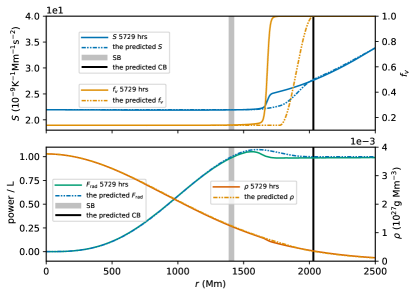
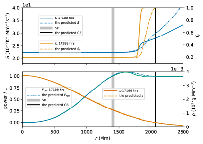
Figure 31: The thermal equilibria predicted by the procedure and the stratifications of M252 (10000x $L_{*}$ & $K_{*}$) at dump 2000 (top) and 6000 (bottom).

In this section, we compare the results of our long-duration simulation, M252, with the equilibrium model state that they imply at two times, dumps 2000 and 6000. The first time comes relatively early in the simulation, and the second very late. The simulation results and their implied equilibrium models are shown in Fig. 31. At each of these two times, we plot the radiative heat conduction flux, normalized by the total luminosity (including the enhancement by a factor 10,000 in this simulation). We also show the radial profile of $f_{\rm V}$ and of the entropy $S$. The simulation results are indicated with solid lines, while the projected equilibrium models are shown with dashed lines.

It is notable how closely the projected equilibria at these well separated times agree. The positions of their convective boundaries agree quite closely, as do their compositional jumps. The entropy curves differ a bit, because the central compositions at these two times differ significantly. In the equilibrium projected from the later time, the compositional jump is broadened from its width in the simulation, and a very significant rise in the entropy inside the foot of this jump causes the entropy signature of the composition jump to become nearly lost in a large, smooth increase. The change in the entropy structure from the simulation result to the implied equilibrium is significant, but the associated change in the radiation diffusion heat flux appears to be a rather minor adjustment. When we consider the earlier of these two times shown in Fig. 31, changes in the entropy structure are much less severe in the implied equilibrium beyond the convective boundary. Once again, we see that the implied equilibrium model inserts quite a substantial entropy rise inside the foot of the compositional jump. As we have pointed out earlier, this feature causes the convection to diminish before the compositional change is encountered, so that mass entrainment rate reduces to nearly zero.

6 Conclusions and Discussion

6.1 Discussion

One might ask if the above 1-D model of the convection zone does not simply exchange the mixing length theory’s (MLT’s) arbitrary paramters and assumptions with other, equally arbitrary parameters and assumptions. We have been guided by our simulations of core convection for a single stellar model near the beginning of its main-sequence life. Nevertheless, this single stellar model poses significant challenges for a 1-D model description. The convection flow is non-local, in that it is dominated by a huge dipole circulation pattern. Also, our 3-D simulations show that a region of penetrative convection develops above the SB in which the radiative energy flux exceeds the star’s total luminosity. We believe that an advantage of our 1-D model, as presented in the previous section, is that the assumptions we make do not require us to calibrate the value of an assumed constant of order unity against observations of the stellar surface with which this constant might be only tenuously related. We do require the determination of the kinetic energy dissipation rate, $\Phi(r)$ in the convection zone, but this does not require calibration against any observations. Instead, we determine this function from theory alone, using the assumption of dynamical equilibrium, the kinetic energy equation reduced to 1D, and a 3-D stellar hydrodynamics code (such as, for example, any in the recently published code comparison study, Andrassy et al., 2022).

We also assume various smoothness constraints on unknown functions inside the region of convective penetration, but we believe that these assumptions are quite natrural. We do assume what we believe is a reasonable location and shape for the jump in composition that must occur very near to the CB. We find very little dependence of our resulting model on where we place $r_{\rm foot}$, the radius at which our assumed sine-wave $f_{\rm V}$ radial profile begins. In Fig. 29, we show the projected equilibrium state using data from run M252’s dump 6000 for 3 different choices of $r_{\rm foot}$, with the middle one being the one we recommend for the model. Perhaps the placement of $r_{\rm foot}$ would matter more at a later stage of evolution, when the jump in $f_{\rm V}$ causes greater change in the composition of the gas. We have also shown in Fig. 30. that the breadth and shape of this rapid increase of $f_{\rm V}$ changes little as the luminosity enhancement factor is increased by as much as a factor of 10.

We believe that the outward motion of the CB can slow very greatly, but we can see no way that entrainment can ever fully stop, except through changes brought about on the nuclear reaction time scale. From this point of view our equilibrium model is an idealization. The jump in $f_{\rm V}$ is responsible for the wiggles in the temperature gradients shown in Fig. 16, yet the radiative heat conduction fluxes shown in Fig. 24 are very smooth as they pass through the region of this jump. This merely shows the power of thermal equilibration. The thermal adjustment cannot remove the jump in $f_{\rm V}$ or the feature in the opacity corresponding to it, but it can nevertheless produce a very smooth thermal conduction flux in this region of radii. Our model, in its present form, addresses core convection. We have not attempted as yet to generalize it to a convective shell. Nor have we attempted to make it time dependent, so that it might describe the creation of a convection zone other than by a sequence of near-equilibrium states.

We note that we have relied heavily on scaling relationships in order to carry out this study with our explicit stellar hydrodynamics code PPMstar. We have argued that the scaling relationships we rely on do hold, and we have produced evidence that they do in the specific instance of this stellar model over a reasonable range of luminosity enhancement factors. It is always possible that the scaling power laws might change in some unexplored regime, or that phenomena that produce the flows we compute might somehow scale with different powers of the luminosity. With the computational tools that we have available at present, widening our exploration to gain more confidence in the scaling relationships is not practical, although we do hope to improve our tools in the future.

6.2 Conclusion

In this work we have performed a series of numerical simulations of 25 $\mathrm{M}_{\odot}$ main sequence stars to investigate the effect of radiation ($P_{\mathrm{rad}}$ and radiative diffusion) on convective and thermal timescales on entrainment, IGWs, and convection. Below is a summary of our main findings.

Entrainment rate at the CB.

By including radiative diffusion enhanced by the same factor as luminosity, we see about a $\sim 30\%$ decrease in the entrainment rate at every luminosity enhancement §3.3. Consequently, the entrainment rate extrapolated to the nominal heating is reduced by about $30\%$ by radiative diffusion, from $1.31\times 10^{-4}$ $\mathrm{M}_{\odot}$/$\mathrm{yr}$ to $9.11\times 10^{-5}$ $\mathrm{M}_{\odot}$/$\mathrm{yr}$. Note that the entrainment is measured in a time window much shorter than the thermal timescale and before the stratification changes dramatically from the initial state.

Damping of the IGWs.

IGWs of small wavelengths are damped by radiative diffusion. Therefore, the vorticity in the radiative envelope converges upon mesh refinement, while it does not do so in the absence of radiative diffusion (§3.4). This behavior may have an impact on IGW mixing in the stable layer.

Thermal equilibrium.

Even in the cases where we scaled the thermal conductivity linearly with luminosity, the entrainment rate we measured was still too large to be consistent with observations. We conclude that our simulations only reach dynamical equilibrium, but the thermal stratification is still adjusting on a thermal timescale. Close to thermal equilibrium, the entrainment rate should drop to a very much lower level. The long time simulation that we carried out develops well defined penetration convection (§4). We identify a mechanism that slows convective boundary mixing and the outward movement of the CB: namely, the composition increase begins where $N^{2}$ is already significantly positive, see Fig. 16. When convection is gradually suppressed by the stable stratification in the penetration region, and the motion is more and more of IGW nature, the time it takes to fully mix increases. This behavior can explain why the entrainment slows down greatly but cannot stop. Thus it is possible that there is always a slow secular change in the composition profile and the stellar stratification.

Behavior of terms in the kinetic energy equation.

The $u\cdot\nabla p_{1}$ term in the kinetic energy equation has a major contribution from the tangential component of the pressure gradient (§4.3). This contribution is significant near the CB, where the flows turn horizontal. This term is determined by the global morphology of the flow and cannot be well approximated solely by the radial component. This discourages attempts at 1D approximations for the kinetic energy equation.

Turbulent kinetic energy dissipation.

In the entropy equation, the turbulent dissipation is about 10 times smaller than the advective entropy flux term and the $(F_{\mathrm{rad}}-F_{\mathrm{nuc}})$ term. Its magnitude does not depend on the physical or numerical viscosity, and we can measure it and get a converged result with modest grid resolutions (§4.3). Nevertheless, an accurate knowledge of the turbulent dissipation rate is required to know the size of the penetrative convection region. Overestimating the dissipation will end up producing convection zones that are unrealistically small. Fortunately, the turbulent dissipation does not vary much inside the SB over a thermal timescale and converges on a grid of $768^{3}$. Hence, only a modest grid (for PPMstar $768^{3}$ or more) and only a few hundred hours of simulated time is needed for the flow to sufficiently adjust inside the SB to give a good measurement of the turbulent dissipation rate that is implied by assuming that the kinetic energy equation is in balance there.

Mixing in the presence of positive $N^{2}$.

From our long time simulations, we observe heat conduction fluxes exceeding the total luminosity and compensating negative convective heat fluxes beyond the SB. These features are recognized as penetrative convection. The compositional jump occurs at all times just inside the CB, and at late times there is very little turbulent flow and mixing there. At late times, efficient convective mixing is spatially separated from the compositional change, and this separation impedes the entrainment of buoyant fluid from above the CB. The spatial separation is caused by local heating of the gas brought about by the declining outward heat flux associated with radiative diffusion in the penetration region, where the radiative flux is approaching the total luminosity from above. This property of the stratification does not present itself in the initial setups we have used, which suggests that our 1D initial state derived from the MESA code model does not characterize convective boundary mixing in a way that is consistent with 3D simulation. We believe this is the reason why very large entrainment rates are always observed early on in our 3D simulations.

A method to determine the convective penetration depth.

We can find a good approximation to the penetration depth as in §5.3 by

1. Integrate the entropy equation forward in radius from the center of the star to the SB, staying on a single adiabat and enforcing hydrostatic equilibrium at each radius.

2. Guess the penetration depth (the radius of the CB) and introduce in the penetration region smooth continuations of the kinetic energy dissipation rate, the radiative heat conduction flux, and the volumetric mixing fraction $f_{\rm V}$.

3. Integrate the entropy equation forward to the provisional CB radius, and then iterate on the penetration depth estimate (steps 2 and 3) until at that radius we find that the radial entropy flux vanishes.

To accomplish the first step and integrate up to the SB, we assume time independence and a well-mixed, adiabatic stratification. The convective entropy flux is then determined, if we know the relatively small rate of kinetic energy dissipation. We may find this rate from a short 3-D simulation of the convection on a relatively coarse grid, or we may interpolate between such simulation results carried out under similar but not identical conditions. We can find the dissipation rate inside the SB even from a non-equilibrium stratification (see Figure 18: the dissipation rate at an early time is very similar to that of a later time much closer to equilibrium). Alternatively, we may estimate the kinetic energy in the convection zone from classical mixing-length theory, or some equivalent approximating model, and then apply a turbulence model to arrive at the rate of kinetic energy dissipation. This approach, however, introduces two free parameters, the mixing length and the scale of the energy-containing turbulent eddies. After guessing the penetration depth, we integrate forward by assuming functional forms for three quantities: the kinetic energy dissipation rate, $\Phi(r)$, the radiative heat conduction flux, $F_{\mathrm{rad}}(r)$, and the volumetric mixing fraction, $f_{\rm V}(r)$, of convection zone gas and gas from the stably stratified envelope above the convection zone. Then we determine the penetration depth, and hence the radius of the CB, by demanding that the convective entropy flux must vanish there.

1. We approximate the radiative heat conduction flux by the unique fifth-order polynomial that is continuously twice differentiable at the SB and that equals the total luminosity at the boundary of the penetration region (CB) with vanishing first and second radial derivatives.

2. We prescribe the functional form of turbulent dissipation in the penetration region as the unique quartic polynomial that is continuously differentiable with vanishing radial derivative at the SB and that vanishes at the CB with vanishing first two radial derivatives.

3. We prescribe the functional form of the volumetric mixing fraction $f_{\rm V}$ in the penetration region as equal to its value at the SB up to a radius $r_{\rm foot}$ and then increasing to unity at the CB with the shape of the sine wave between its minimum and maximum at argument values $-\pi/2$ and $\pi/2$. We choose $r_{\rm foot}$ as the radius at which the local heating from the declining radiative heat conduction flux has its maximum value.

4. Finally, we require the entropy flux to vanish at the CB.

Dependence of the penetration depth on luminosity enhancement factor.

In the limit of large convection efficiency, the thermal relaxation is accelerated by enhancement of the luminosity and the radiative diffusion by a common factor, so long as this enhancement keeps the Mach number of the convection flow small, so that the character of the flow is not much changed. In the equilibrium that is reached, the penetration depth depends upon the radiative heat conduction flux, which establishes a positive entropy gradient in the penetration region, and the turbulent dissipation of kinetic energy, which together determine in a time-independent equilibrium the radial entropy flux, which must vanish at the CB. All these terms that must balance in equilibrium in this region scale linearly with the luminosity under these conditions (see similar arguments in §4.3.4, Fig. 30). Hence the penetration depth for an enhanced luminosity should equal the penetration depth for the actual star. We have tested this scaling law for enhancement factors of 1000 and greater, but, at present, technical issues prevent our demonstrating this scaling law for smaller enhancement factors.

Using this procedure, we see that the penetration depth depends upon our estimate of the turbulent convective energy dissipation rate and its functional form in the penetration region. This dissipation rate cannot be determined directly, without the use of a model, in a 1-D stellar evolution computation. We find that the penetration depth estimate increases/decreases by 30 $\mathrm{Mm}$ if we decrease/increase the turbulent dissipation everywhere by $5\%$ for our particular stellar model. We note that as the convection flow nears equilibrium, the convective mixing, as indicated by the size of $\Phi(r)$, declines near the CB to values very close to zero, which reduces the convective boundary mixing dramatically and allows the outward motion of the CB to very nearly cease. The thermal adjustment in the thin region just before the CB where the composition changes results in a smooth, nearly featureless form there for $F_{\mathrm{rad}}(r)$, although features do appear there in both the temperature and the opacity.

Future work.

In future work, we will expand the cases we have considered, and this will no doubt lead to refinements of the recommended procedure. However, we argue that finding the CB location is strictly impossible without knowing the kinetic energy dissipation as a function of radius, and knowing that is impossible in a 1D simulation without the use of a model.

References

- Aerts et al. (2019) Aerts, C., Mathis, S., & Rogers, T. M. 2019, Annual Review of Astronomy and Astrophysics, 57, 1, doi: 10.1146/annurev-astro-091918-104359
- Anders et al. (2022) Anders, E. H., Jermyn, A. S., Lecoanet, D., & Brown, B. P. 2022, ApJ, 926, 169, doi: 10.3847/1538-4357/ac408d
- Andrassy et al. (2020) Andrassy, R., Herwig, F., Woodward, P., & Ritter, C. 2020, MNRAS, 491, 972, doi: 10.1093/mnras/stz2952
- Andrassy et al. (2022) Andrassy, R., Higl, J., Mao, H., et al. 2022, A&A, 659, A193, doi: 10.1051/0004-6361/202142557
- Arnett et al. (2008) Arnett, D., Meakin, C., & Young, P. A. 2008, The Astrophysical Journal, 690, 1715
- Arnett et al. (2009) Arnett, D., Meakin, C., & Young, P. A. 2009, ApJ, 690, 1715, doi: 10.1088/0004-637X/690/2/1715
- Arnett et al. (2015) Arnett, W. D., Meakin, C., Viallet, M., et al. 2015, The Astrophysical Journal, 809, 30
- Baraffe et al. (2017) Baraffe, I., Pratt, J., Goffrey, T., et al. 2017, The Astrophysical Journal Letters, 845, L6
- Baraffe et al. (2021) Baraffe, I., Pratt, J., Vlaykov, D. G., et al. 2021, A&A, 654, A126, doi: 10.1051/0004-6361/202140441
- Blouin et al. (2023) Blouin, S., Mao, H., Herwig, F., et al. 2023, arXiv preprint arXiv:2303.07332
- Böhm-Vitense (1958) Böhm-Vitense, E. 1958, ZAp, 46, 108
- Bowman et al. (2020) Bowman, D. M., Burssens, S., Simón-Díaz, S., et al. 2020, A&A, 640, A36, doi: 10.1051/0004-6361/202038224
- Canuto & Mazzitelli (1991) Canuto, V., & Mazzitelli, I. 1991, The Astrophysical Journal, 370, 295
- Chan & Sofia (1989) Chan, K. L., & Sofia, S. 1989, The Astrophysical Journal, 336, 1022
- Cox & Giuli (1968) Cox, J. P., & Giuli, R. T. 1968, Principles of Stellar Structure. Vol. 1: Physical Principles (New York)
- Davis et al. (2018) Davis, A., Jones, S., & Herwig, F. 2018, MNRAS, 484, 3921
- Denissenkov et al. (2012) Denissenkov, P. A., Herwig, F., Bildsten, L., & Paxton, B. 2012, ApJ, 762, 8
- Edelmann et al. (2019) Edelmann, P. V. F., Ratnasingam, R. P., Pedersen, M. G., et al. 2019, ApJ, 876, 4
- Freytag et al. (1996) Freytag, B., Ludwig, H. G., & Steffen, M. 1996, A&A, 313, 497
- Frisch (1995) Frisch, U. 1995, Turbulence: The Legacy of A. N. Kolmogorov (Cambridge University Press), doi: 10.1017/CBO9781139170666
- Garaud et al. (2017) Garaud, P., Gagnier, D., & Verhoeven, J. 2017, ApJ, 837, 133, doi: 10.3847/1538-4357/837/2/133
- Gilet et al. (2013) Gilet, C., Almgren, A. S., Bell, J. B., et al. 2013, ApJ, 773, 137
- Grinstein et al. (2007) Grinstein, F. F., Margolin, L. G., & Rider, W. J. 2007, Implicit large eddy simulation, Vol. 10 (Cambridge university press Cambridge)
- Herwig et al. (2000) Herwig, F., Blöcker, T., & Driebe, T. 2000, in The changes in abundances in AGB stars, ed. F. D’Antona & R. Gallino, Vol. 71, 745
- Herwig et al. (2006) Herwig, F., Freytag, B., Hueckstaedt, R. M., & Timmes, F. X. 2006, ApJ, 642, 1057
- Herwig et al. (2023) Herwig, F., Woodward, P. R., Mao, H., et al. 2023, MNRAS, doi: 10.48550/arXiv.2303.05495
- Higgins & Vink (2019) Higgins, E. R., & Vink, J. S. 2019, A&A, 622, A50, doi: 10.1051/0004-6361/201834123
- Higl et al. (2021) Higl, J., Mueller, E., & Weiss, A. 2021, Astronomy & Astrophysics, 646, A133
- Hurlburt et al. (1986) Hurlburt, N. E., Toomre, J., & Massaguer, J. M. 1986, The Astrophysical Journal, 311, 563. https://ui.adsabs.harvard.edu/abs/1986ApJ...311..563H/abstract
- Hurlburt et al. (1994) Hurlburt, N. E., Toomre, J., Massaguer, J. M., & Zahn, J.-P. 1994, The Astrophysical Journal, 421, 245
- Iglesias & Rogers (1996) Iglesias, C. A., & Rogers, F. J. 1996, ApJ, 464, 943, doi: 10.1086/177381
- Jones et al. (2017) Jones, S., Andrássy, R., Sandalski, S., et al. 2017, MNRAS, 465, 2991
- Kaiser et al. (2020) Kaiser, E. A., Hirschi, R., Arnett, W. D., et al. 2020, MNRAS, 496, 1967, doi: 10.1093/mnras/staa1595
- Kippenhahn et al. (1990) Kippenhahn, R., Weigert, A., & Weiss, A. 1990, Stellar structure and evolution, Vol. 192 (Springer)
- Korre & Featherstone (2021) Korre, L., & Featherstone, N. A. 2021, The Astrophysical Journal, 923, 52
- Lecoanet & Quataert (2013) Lecoanet, D., & Quataert, E. 2013, Monthly Notices of the Royal Astronomical Society, 430, 2363
- Maeder (1976) Maeder, A. 1976, A&A, 47, 389
- Meakin & Arnett (2007) Meakin, C. A., & Arnett, W. D. 2007, ApJ, 667, 448
- Michielsen et al. (2021) Michielsen, M., Aerts, C., & Bowman, D. M. 2021, Astronomy & Astrophysics, 650, A175, doi: 10.1051/0004-6361/202039926
- Michielsen et al. (2019) Michielsen, M., Pedersen, M. G., Augustson, K. C., Mathis, S., & Aerts, C. 2019, A&A, 628, A76
- Moravveji et al. (2015) Moravveji, E., Aerts, C., Papics, P. I., Triana, S. A., & Vandoren, B. 2015, A&A, 580, A27
- Pasetto et al. (2014) Pasetto, S., Chiosi, C., Cropper, M., & Grebel, E. 2014, Monthly Notices of the Royal Astronomical Society, 445, 3592
- Paxton et al. (2010) Paxton, B., Bildsten, L., Dotter, A., et al. 2010, The Astrophysical Journal Supplement Series, 192, 3, doi: 10.1088/0067-0049/192/1/3
- Paxton et al. (2013) Paxton, B., Cantiello, M., Arras, P., et al. 2013, The Astrophysical Journal Supplement Series, 208, 4, doi: 10.1088/0067-0049/208/1/4
- Paxton et al. (2015) Paxton, B., Marchant, P., Schwab, J., et al. 2015, The Astrophysical Journal Supplement Series, 220, 15, doi: 10.1088/0067-0049/220/1/15
- Pinçon et al. (2016) Pinçon, C., Belkacem, K., & Goupil, M. 2016, Astronomy & Astrophysics, 588, A122
- Porter & Woodward (1994) Porter, D. H., & Woodward, P. R. 1994, The Astrophysical Journal Supplement Series, 93, 309, doi: 10.1086/192057
- Porter et al. (2000) Porter, D. H., Woodward, P. R., & Jacobs, M. L. 2000, in New York Academy Sciences Annals, Vol. 898, Astrophysical Turbulence and Convection, ed. J. R. Buchler & H. Kandrup, 1–+
- Porter et al. (1998) Porter, D. H., Woodward, P. R., & Pouquet, A. 1998, Physics of Fluids, 10, 237
- Pratt et al. (2017) Pratt, J., Baraffe, I., Goffrey, T., et al. 2017, Astronomy & Astrophysics, 604, A125
- Pratt et al. (2020) —. 2020, Astronomy & Astrophysics, 638, A15
- Press (1981) Press, W. H. 1981, Astrophysical Journal, 245, 286
- Prialnik (2000) Prialnik, D. 2000, An introduction to the theory of stellar structure and evolution (Cambridge University Press)
- Ribas et al. (2000) Ribas, I., Jordi, C., & Gimenez, A. 2000, Monthly Notices of the Royal Astronomical Society, 318, L55 , doi: 10.1046/j.1365-8711.2000.04035.x
- Rogers & McElwaine (2017) Rogers, T. M., & McElwaine, J. N. 2017, ApJ, 848, L1, doi: 10.3847/2041-8213/aa8d13
- Roxburgh (1989) Roxburgh, I. 1989, Astronomy and Astrophysics, 211, 361
- Roxburgh (1992) —. 1992, Astronomy and Astrophysics, 266, 291
- Salaris & Cassisi (2017) Salaris, M., & Cassisi, S. 2017, Royal Society Open Science, 4, 170192
- Schaller et al. (1992) Schaller, G., Schaerer, D., Meynet, G., & Maeder, A. 1992, Astronomy and Astrophysics Supplement Series, 96, 269
- Scott et al. (2021) Scott, L., Hirschi, R., Georgy, C., et al. 2021, Monthly Notices of the Royal Astronomical Society, 503, 4208
- Staritsin (2013) Staritsin, E. 2013, Astronomy Reports, 57, 380
- Stephens et al. (2021) Stephens, D., Herwig, F., Woodward, P., et al. 2021, MNRAS, 504, 744, doi: 10.1093/mnras/stab500
- Sukhbold & Woosley (2014) Sukhbold, T., & Woosley, S. E. 2014, ApJ, 783, 10, doi: 10.1088/0004-637X/783/1/10
- Thompson et al. (2023) Thompson, W., Herwig, F., Woodward, P. R., et al. 2023, MNRAS, resubmitted, arXiv:2303.06125, doi: 10.48550/arXiv.2303.06125
- Tkachenko et al. (2020) Tkachenko, A., Pavlovski, K., Johnston, C., et al. 2020, A&A, 637, A60, doi: 10.1051/0004-6361/202037452
- Townsend (1958) Townsend, A. A. 1958, Journal of Fluid Mechanics, 4, 361, doi: 10.1017/S0022112058000501
- Trampedach et al. (2014) Trampedach, R., Stein, R. F., Christensen-Dalsgaard, J., Nordlund, A., & Asplund, M. 2014, Monthly Notices of the Royal Astronomical Society, 445, 4366, doi: 10.1093/mnras/stu2084
- Wieczorek & Meschede (2018) Wieczorek, M. A., & Meschede, M. 2018, Geochemistry, Geophysics, Geosystems, 19, 2574, doi: 10.1029/2018GC007529
- Woodward (1986) Woodward, P. R. 1986, in Astrophysical Radiation Hydrodynamics, ed. K.-H. A. Winkler & M. L. Norman, Vol. 188 (Dordrecht: Springer), 245–326. https://doi.org/10.1007/978-94-009-4754-2_8
- Woodward et al. (2015) Woodward, P. R., Herwig, F., & Lin, P.-H. 2015, ApJ, 798, 49
- Woodward & Porter (2006) Woodward, P. R., & Porter, D. H. 2006, in International Workshop on Applied Parallel Computing, Springer, 1074–1083
- Xiong (1986) Xiong, D.-r. 1986, Astronomy and Astrophysics, 167, 239
- Zahn (1974) Zahn, J. P. 1974, in Stellar Instability and Evolution, ed. P. Ledoux, A. Noels, & A. W. Rodgers, Vol. 59, 185
- Zahn (1989) Zahn, J.-P. 1989, Astronomy and Astrophysics, 220, 112
- Zahn et al. (1997) Zahn, J. P., Talon, S., & Matias, J. 1997, A&A, 322, 320. https://arxiv.org/abs/astro-ph/9611189