Pattern formation by non-dissipative arrest of turbulent cascades

Abstract

Fully developed turbulence is a universal and scale-invariant chaotic state characterized by an energy cascade from large to small scales where the cascade is eventually arrested by dissipation. In this Letter, we show how to harness these seemingly structureless turbulent cascades to generate patterns. Conceptually, pattern or structure formation entails a process of wavelength selection: patterns typically arise from the linear instability of a homogeneous state. By contrast, the mechanism we propose here is fully non-linear and triggered by a non-dissipative arrest of turbulent cascades. Instead of being dissipated, energy piles up at intermediate scales. Using a combination of theory and large-scale simulations, we show that the tunable wavelength of these cascade-induced patterns is set by a non-dissipative transport coefficient called odd or gyro viscosity. This non-dissipative viscosity is ubiquitous in chiral systems ranging from plasmas, bio-active media and quantum fluids. Beyond chiral fluids, cascade-induced pattern formation could occur in natural systems including oceanic and atmospheric flows, planetary and stellar plasma such as the solar wind, as well as in industrial processes such as the pulverization of objects into debris or in chemistry and biology where the coagulation of droplets can be interrupted at a tunable scale.

Fully-developed turbulence is a highly chaotic non-equilibrium state in which energy is transferred across scales through a non-linear mechanism known as a turbulent cascade [1, 2, 3, 4, 5, 6]. Heuristically, large eddies, typically created by the injection of energy at macroscopic scales, break-up into smaller and smaller eddies. This energy transfer towards small scales, called a direct or forward cascade, is eventually arrested by dissipation (Fig. 1a). Away from the scales at which energy is injected and dissipated, turbulence is universal and scale invariant.

We start by asking an almost paradoxical question: can we harness turbulence to generate patterns? Our approach to tackle this task rests on the simple observation that different classes of turbulent cascades exist [4]. For example, turbulence in two-dimensional and rotating fluids has a tendency to transfer energy towards larger scales in what is known as an inverse cascade (Fig. 1b). We can then consider what happens when a direct cascade is combined with an inverse cascade. In this situation, represented in Fig. 1c, energy is transferred to an intermediate length scale $k_{\text{c}}^{-1}$ ($k$ are wavenumbers, so their inverses are lengths) both from smaller and larger scales, depending on where energy is injected. As a consequence of this energy accumulation, we expect the emergence of structures with characteristic size $k_{\text{c}}^{-1}$. This ‘spectral condensation’ at intermediate scales requires the mechanism responsible for arresting both cascades to be non-dissipative. As we shall see, Nature has found a very elegant solution to this problem: a viscosity that does not dissipate energy, variously known as odd viscosity [7], Hall viscosity [8, 9, 10] or gyroviscosity [11, 12, 13], see Ref. [14] for a review.

Before delving into concrete realizations, let us compare and contrast this scenario with usual mechanisms of pattern formation, represented in Fig. 1d. In the standard picture of pattern formation [15, 16], patterns arise from the linear instability of a homogeneous system: the length scale $k_{\text{c}}^{-1}$, corresponding to the maximum of the growth rate $\sigma(k)$, is selected because the corresponding mode grows faster, and gives the characteristic size of the emerging pattern. While non-linearities are important in saturating the growth and selecting the precise shape of the pattern, they only play a secondary role, once the linear instability has set in. This paradigm has been very successful in many areas of science. In the context of turbulent fluids, for instance, it is believed to describe laminar/turbulent patterns near the onset of turbulence [17, 18, 19, 20]. By contrast, in the cascade-induced mechanism of pattern formation shown in Fig. 1c, non-linearities play the central role — it is the non-linear interaction between modes that gives rise to the turbulent cascade in the first place.

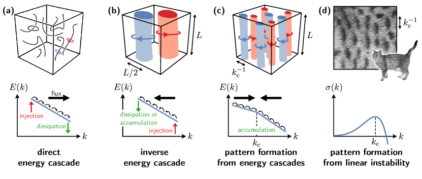
Figure 1: Cascade-induced pattern formation. (a) Direct energy cascade: in a turbulent 3D fluid, energy injected at large scales (red arrow) is transferred to smaller and smaller length scales (black arrows) as vortices break up to microscopic length scales where dissipation occurs (green arrow). This mechanism is intrinsically nonlinear: it relies on triadic couplings between the modes of the system. (b) Inverse energy cascade: in a turbulent 2D fluid, or in a rotating 3D fluid, there is instead a transfer of energy from the scale where energy is injected (red arrow) to larger and larger scales, where energy is either dissipated or piles up at the largest scale available (green arrow), the size of the system. Correspondingly, vortices merge together until only a positive and a negative vortex remain, both of which have approximately half the size $L$ of the system. Inverse cascades can also arise in 3D from rotation or mirror symmetry breaking [4, 21, 22]. (c) In an hypothetical situation where a direct and an inverse cascades can be put together in the right order (black arrows in the figure), energy will be transferred to an intermediate length scale $k_{\text{c}}^{-1}$, leading to the appearance of structure with a characteristic size $k_{\text{c}}^{-1}$ independent of the size $L$ of the system. This non-linear wavelength selection mechanism relying on combined turbulent cascades can be seen as an instance of pattern formation. (d) Standard pattern formation from a linear instability: the wavelength $k_{\text{c}}^{-1}$ corresponding to the most unstable linear mode (i.e., the one with the largest growth rate $\sigma(k)$) is selected. This is a linear mechanism, even though nonlinearities play a crucial role in saturating and modifying the instability. As an example, we have shown patterns on the fur of a cat.

Turbulence with odd viscosity. We start with the three-dimensional incompressible Navier-Stokes equations that govern the dynamics of simple fluids

$$\rho D_{t}v_{i}=-\partial_{i}P+\eta_{ijk\ell}\partial_{j}\partial_{\ell}v_{k}+f_{i}(t,\bm{x})$$ (1)

with the incompressibility condition $\partial_{i}v_{i}=0$, in which $\bm{v}(t,\bm{x})$ is the velocity field, $\rho$ is the density, $P$ is the pressure, $\eta_{ijk\ell}$ is the viscosity tensor, $D_{t}=(\partial_{t}+v_{k}\partial_{k})$ is the convective derivative, $\partial_{k}=\partial/\partial x_{k}$, and $f_{i}(t,\bm{x})$ is an external forcing representing energy injection. In typical fluids such as water, the viscous term in Eq. (1) reads $\eta\Delta\bm{v}$.

In order to realize the mixed cascade of Fig. 1c, we first need to turn a direct cascade into an inverse cascade. This can be achieved by simply rotating the fluid at high velocities (Fig. 2; see Refs. [2, 4]): the Coriolis force $\bm{f}_{\bm{\Omega}}=2\rho\bm{\Omega}\times\bm{v}$ (where $\bm{\Omega}$ is the rotation vector and $\times$ is the vector product), added in the right-hand side of the Navier-Stokes equation (1), leads to an alignment of the vortex lines with the rotation axis. In addition, energy is not injected nor dissipated by the Coriolis force. As the rotation speed increases, the vortex tangle becomes more and more polarized, which induces a two-dimensionalization of the flow and an inverse energy cascade similar to the case of 2D fluids, eventually leading to the condensation of two vortices of opposite vorticity at the size of the system (Fig. 2b,c).

For our purpose, however, we need an inverse cascade at large wavevectors only: this suggests a gradient term in the Navier-Stokes equation, like the viscosity term, but with the additional requirement that it does not dissipate so we can have energy pile-up, i.e. a condensate, at the length scale $k_{\text{c}}^{-1}$. All we need to do is to allow an antisymmetric part in the viscosity tensor

$$\eta_{ijk\ell}\neq\eta_{k\ell ij}$$ (2)

in Eq. (1). Like the Coriolis force, the antisymmetric part of the viscosity tensor does not contribute to energy dissipation or injection as it drops out from the energy balance equation [23]. The corresponding viscosities are called odd, Hall, or gyro viscosities, and they typically arise in systems breaking time-reversal and inversion symmetry at the microscopic scale [7, 24, 14]. Odd viscosities have been experimentally measured in polyatomic gases under magnetic fields [25, 26], spinning colloids [27], and magnetized electron fluids [10]. They have also been predicted in systems including fluids under rotation [28], magnetized plasma [11, 12, 13], chiral superfluids [29], vortex matter [30], sheared granular gases [31], assemblies of spinning objects [32, 33, 34, 35], and circle swimming bacteria [36, 37]. As isotropic 3D systems always have $\eta_{ijk\ell}=\eta_{k\ell ij}$, we assume that the system is invariant under rotation about the $z$-axis (cylindrical symmetry), see [23]. The most general Navier-Stokes equation with odd viscosities compatible with this symmetry is given in the Methods. For concreteness, we focus in the main text on a simple case where the Navier-Stokes equations read

$$\rho D_{t}\bm{v}=-\nabla\tilde{P}+\eta\Delta\bm{v}+\eta_{\text{odd}}\bm{e}_{z}\times\Delta\bm{v}+\bm{f}(t,\bm{x})$$ (3)

in which $\eta$ is the familiar shear viscosity, $\eta_{\text{odd}}$ is a particular combination of odd viscosities (see Methods Eq. 16), and $\bm{e}_{z}$ is the unit vector along $z$. We have defined an effective pressure $\tilde{P}=P+\eta_{\text{odd}}\omega_{z}$ where $\bm{\omega}=\nabla\times\bm{v}$ is the vorticity. This modification of the pressure is unimportant because we consider an incompressible fluid with periodic boundary conditions. The odd viscosity term $\eta_{\text{odd}}\bm{e}_{z}\times\Delta\bm{v}$ is very similar to the Coriolis force. Both are non-dissipative and anisotropic, in this case with axes along the $z$-direction. The main difference is the additional Laplacian, which ensures that its action vanishes at large length scales (small wavenumber). In wavenumber space, the odd viscosity term in Eq. (3) reads $-\eta_{\text{odd}}k^{2}\bm{e}_{z}\times\bm{v}(\bm{k})$ and can be thought of as a wavenumber-dependent rotation ($\bm{k}$ is the wavevector and $k=\lVert\bm{k}\rVert$).

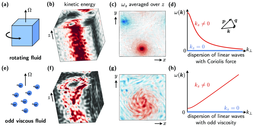
Figure 2: Two-dimensionalization in rotating and odd turbulence. We compare (a-d) a turbulent fluid flow rotating with high frequency $\bm{\Omega}$ and (e-h) a fluid with strong odd (dissipationless) viscosity. The odd fluid is composed of constituents that all spin in one direction. Both fluids are anisotropic, with $\bm{\Omega}$ pointing along the $z$-axis in each system. (b,f) The kinetic energy is concentrated in a system-size condensate. (c, g) The vertical vorticity ($\omega_{z}$) is averaged over $z$ to highlight vertical coherence in both systems. (d,h) We plot the dispersion of inertial waves in a rotating fluid (panel d) and of odd waves in an odd fluid (panel h, see Eq. (7)). These anisotropic dispersion relations hint at an inverse cascade: modes with no vertical variation ($k_{z}=0$, blue lines) do not support waves, while modes with non-zero horizontal wavenumber have a finite frequency (red lines) and therefore quickly decorrelate, which results in a two-dimensionalization of the flow in both fluids. Panels b-c and f-g are obtained by numerical simulations of the Navier-Stokes equations, see main text.

Two-dimensionalization: Taylor-Proudman argument. The two-dimensionalization of turbulence in fluids under rotation can be qualitatively understood from the so-called Taylor-Proudman argument [38, 39]. When both inertial and viscous forces can be neglected with respect to the Coriolis force in a stationary flow, the pressure force balances the Coriolis force ($2\rho\Omega\bm{e}_{z}\times\bm{v}=\nabla P$). Taking the curl of the Navier-Stokes equation and using incompressibility then gives $\partial_{z}\bm{v}=0$, heralding the two-dimensionalization of the flow, as the velocity no longer depends on $z$. This is known as the Taylor-Proudman theorem [38, 39] (see e.g. [2, § 9.2.2] for a pedagogical discussion). Although in a turbulent flow, the inertial term is not negligible, vertical variations of the turbulent flow field are still largely suppressed under strong rotation, resulting in a quasi-2D state, see Fig. 2a-c.

We now extend this argument to the case of odd fluids (Fig. 2e-g) in which the Coriolis force is replaced with odd viscosity. Under the same assumptions as before, we find $\eta_{\text{odd}}\bm{e}_{z}\times\Delta\bm{v}=\bm{\nabla}P$. Taking the curl of this equation and using incompressibility, we get (see Methods)

$$\eta_{\text{odd}}\,\partial_{z}\Delta\bm{v}=\bm{0}.$$ (4)

Compared to the traditional Taylor-Proudman theorem, Eq. (4) has an extra Laplacian: it shows that the variations of $\Delta\bm{v}$ are suppressed in the $z$ direction. Similar to rotating turbulence, this suggests two-dimensionalization of the flow, but in a way that is enforced more strongly on small scales, owing to the Laplacian. Similar variations of the Taylor-Proudman theorem (4) hold for all odd viscosities compatible with cylindrical symmetry; we provide a derivation in the Methods. Based on this modified theorem, we can expect fluids with strong odd viscosity to exhibit features similar to quickly rotating fluids such as the equivalent of Taylor columns and quasi-two-dimensionalization [2].

A qualitative comparison between turbulence under strong rotation and turbulence under strong odd viscosity provided in Fig. 2 (resulting from our direct numerical simulations of the Navier-Stokes equations, see Methods for details) confirms these expectations.

Energy transfer and odd waves. We now turn to the analysis of the turbulent cascade. To do so, let us introduce the energy spectrum $E(t,\bm{k})=\frac{1}{2}\lVert\bm{v}(t,\bm{k})\rVert^{2}$ describing the distribution of energy among scales [2]. Starting from the Fourier-transformed Navier-Stokes equation and multiplying with $\bm{v}^{*}(t,\bm{k})$ (the star denotes complex conjugation), we find the energy budget equation

$$\partial_{t}E=-2\nu k^{2}E-T+F$$ (5)

where $\nu=\eta/\rho$ is the kinematic viscosity, and in which

$$T(\bm{k},t)=\textrm{Im}\sum_{\bm{p}+\bm{q}=\bm{k}}{v}_{i}^{*}(\bm{k},t)P_{ij}(\bm{k})q_{\ell}{v}_{\ell}(\bm{p},t){v}_{j}(\bm{q},t)$$ (6)

describes the non-linear energy transfer between scales, while $F=\bm{v}^{*}\cdot\bm{f}$ corresponds to energy injection by the forcing term $\bm{f}$. In addition, $P_{ij}(\bm{k})=\delta_{ij}-k_{i}k_{j}/k^{2}$ is the projector on incompressible flows. In Eq. (6), the sum runs on momenta $\bm{p}$ and $\bm{q}$ such that $\bm{p}+\bm{q}=\bm{k}$ (see inset of Fig. 2d). The tuple $(\bm{p},\bm{q},\bm{k})$ is known as a triad. Here, we focus on the stationary energy spectrum $E(\bm{k})$ obtained by setting $\partial_{t}E=0$ in Eq. (5), and consider its spherical average $E(k)$.

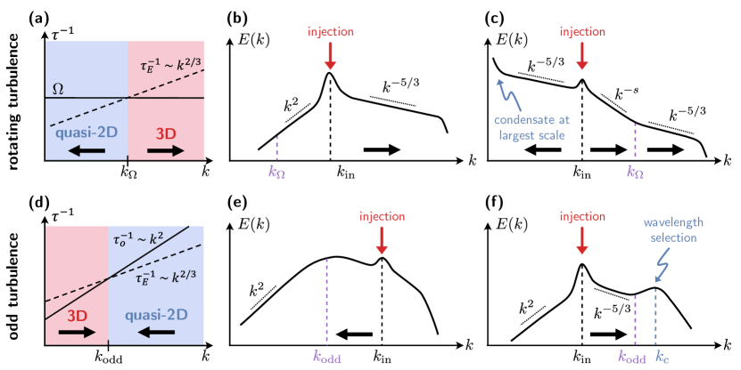
Figure 3: Scaling theory of rotating and odd turbulence. We compare features of (a-c) rotating and (d-f) odd turbulence. (a,d) A comparison of time scales predicts cascade direction. In a rotating fluid (panel a), since the eddy turnover frequency scales as $\tau_{E}^{-1}\sim k^{2/3}$, the rotating fluid is quasi-2D at small scales (blue region) and isotropic at small scales (once $\tau_{E}^{-1}>\Omega$, red region). In an odd fluid (panel d), since $\tau_{\text{odd}}^{-1}=\omega(k)\sim k^{2}$, we expect the odd fluid to remain quasi-2D at large wavenumbers (blue region), and instead isotropize at low $k$, when $\tau_{E}^{-1}>\tau_{\text{odd}}^{-1}$ (red region). The crossover point defines the odd viscosity length scale $k_{\text{odd}}$, in analogy to the Zeman scale $k_{\Omega}$ in rotating fluids. The direction of the energy flux in indicated by the black arrows. Cascades in the energy spectra when the injection scale is smaller (b,e) and larger (c,f) than the characteristic scale. In the rotating fluid, there is a direct cascade of energy below the rotation (Zeman) scale (b), and an inverse cascade above (c). In the odd fluid, we expect the situation to be reversed. Following the timescale argument in (d), energy cascades directly for wavenumbers below $k_{\text{odd}}$ (f) and inversely above (e), causing a pile up of energy at the odd viscosity length scale and arresting both cascades. The pileup is eventually saturated by viscous dissipation, leading to a bump in the energy spectrum at a characteristic scale $k_{\text{c}}$, compared to the spectrum that would occur without odd viscosity.

Equation (5) is not modified by odd viscosity, because it is not dissipative. Nevertheless, odd viscosity does indirectly affect the nonlinear energy transfer. To see that, let us first identify the natural modes of the odd fluid by performing a linear stability analysis about the fluid at rest. We find that the complex growth rate is (see Methods)

$$\sigma(\bm{k})+\text{i}\omega(\bm{k})=-\nu k^{2}\pm i\nu_{\text{odd}}k_{z}\mathinner{\!\left\lvert k\right\rvert}$$ (7)

where we have defined $\nu_{\text{odd}}=\eta_{\text{odd}}/\rho$ and in which $\sigma(\bm{k})$ is the growth/decay rate of the perturbations and $\omega(\bm{k})$ is their frequency. This dispersion relation is shown in Fig. 2h (compare with the case of rotating fluids in panel d). The odd waves with dispersion $\omega(\bm{k})$ given by Eq. (7) are the equivalent for odd fluids of the so-called inertial waves in rotating fluids, in which the Coriolis force leads to a dispersion relation $\omega_{\bm{\Omega}}(\bm{k})=\pm 2\bm{\Omega}\cdot\bm{k}/k$ (see e.g. [2, § 9.2.3]). Unlike normal fluids (where $\eta_{\text{odd}}=0$), and similar to fluids under rotation, fluids with odd viscosity support decaying wave solutions. In contrast with fluids under rotation, for which $\omega_{\bm{\Omega}}(\bm{k})=\pm 2\Omega k_{z}/k$ saturates, here the frequency keeps increasing with $k_{z}$.

The physical significance of these fast waves is that they decorrelate the triadic interactions that compose the non-linear energy transport in the turbulent flow (inset of Fig. 2d), because the corresponding modes quickly go out of phase with each other. From the expression (6) of the non-linear energy transfer, we find that

$$T(\bm{k},t)\sim\exp(-\text{i}[\omega(\bm{p})+\omega(\bm{q})+\omega(\bm{k})]t).$$ (8)

This quantity averages to zero in one period, unless the resonance condition $\omega(\bm{p})+\omega(\bm{q})+\omega(\bm{k})=0$ is satisfied. The modes with $k_{z}=0$ all have $\omega=0$ (blue line in Fig. 2h), so they do not decorrelate. These 2D modes form the so-called slow manifold that contributes to most of the non-linear energy transfer. In addition, isolated triads with $k_{z}\neq 0$ can also satisfy the resonance condition. In the case of rotating turbulence, it is understood that resonant triads primarily transfer energy from the 3D modes to quasi-2D slow manifold with $k_{z}=0$, leading to an accumulation of energy in the slow manifold, enhancing the two-dimensionalization of the flow [40, 41, 42, 4]. There, at large wavenumbers, however, triadic interactions between the fast 3D modes are responsible for a direct cascade. Here, the dispersion relation is noticeably different: $\omega(\bm{k})$ does not saturate when $k_{z}$ increases, and it increases with $k_{\perp}$ ($\bm{k}_{\perp}$ is the part of the wavevector orthogonal to the $z$ axis, and $k_{\perp}=\lVert\bm{k}_{\perp}\rVert$). Therefore, we expect a markedly different phenomenology, which we now analyze using scaling arguments.

Scaling theory of the arrested cascade. In a turbulent flow, the lifespan of a typical eddy is called the turnover time $\tau_{E}$, and its inverse is called the eddy turnover frequency. The mechanisms transferring energy across scales occur over a few turnover times, so the average of the non-linear energy transfer (8) should be performed over $\tau_{E}$. To analyze whether the effect of odd viscosity is important, we therefore compare the eddy turnover frequency $\tau_{E}^{-1}$ with the frequency $\omega(\bm{k})$ of the waves given in Eq. (7). Assuming $k_{z}\sim k$ because of the two-dimensionalization, we look for the scale $k_{\text{odd}}$ such that $\omega(k=k_{\text{odd}})=\tau_{E}^{-1}(k=k_{\text{odd}})$. Estimating the eddy turnover frequency $\tau_{E}^{-1}\sim k^{2/3}\epsilon^{1/3}$ from the rate of dissipation of energy at small scales $\epsilon$ (see e.g. [2]), we find

$$k_{\text{odd}}\equiv\epsilon^{1/4}\nu_{\text{odd}}^{-3/4}.$$ (9)

When $k\gg k_{\text{odd}}$, the effect of odd viscosity is important: $T$ in Eq. (8) averages to zero over the lifespan of a typical eddy, and we expect quasi-2D behavior. In contrast, when $k\ll k_{\text{odd}}$, the effect of odd viscosity is negligible and we expect normal 3D behavior. This is summarized in Fig. 3d. In the case of rotating turbulence, the same analysis leads to the so-called Zeman scale [43, 44]: the wavenumber $k_{\Omega}=\Omega^{3/2}\epsilon^{-1/2}$. In rotating turbulence, since $\Omega$ is $k$-independent, it dominates the eddy turnover frequency at small wavenumbers, giving rise to a quasi-2D inverse cascade at large scales, but it is exceeded by $\tau_{E}^{-1}$ at wavenumbers above the Zeman scale, leading to small scale isotropization and a direct cascade (Fig. 3a).

Comparing panels a and d of Fig. 3 shows that the order of the 3D behavior (with a direct cascade) and the quasi-2D behavior (with an inverse cascade) are permuted in rotating and odd fluids, because of the $k^{2}$ scaling of $\omega(\bm{k})$ in odd fluids. As a consequence, both a direct and an inverse cascade are thus arrested when they approach the odd viscosity wavenumber $k_{\text{odd}}$ (Fig. 3e,f). Since odd viscosity is non-dissipative, kinetic energy can be expected to pile up into a condensate around $k_{\text{odd}}$ until its growth is stopped by the regular dissipation from the normal shear viscosity (first term in the RHS of Eq. (5)).

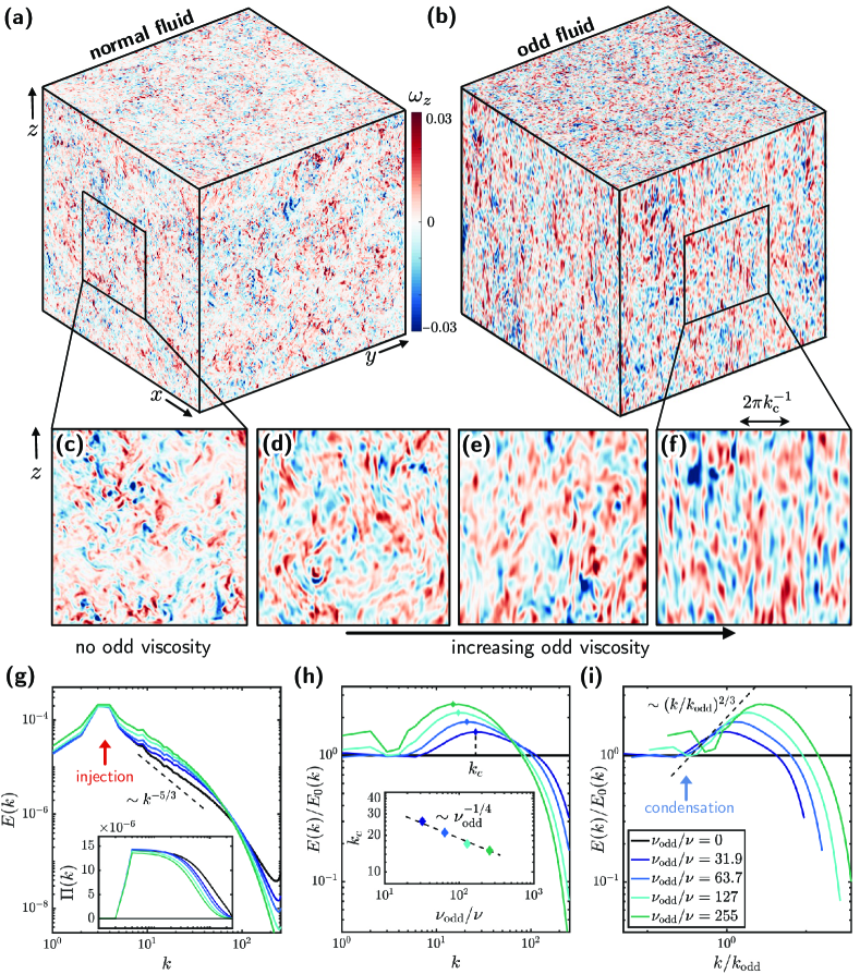
Figure 4: Wavelength selection in numerical direct cascade. We show the vorticity in the $z$-direction ($\omega_{z}$) obtained by direct simulations of the Navier-Stokes equation without and with odd viscosity in panels a-f In the absence of odd viscosity (a,c), vortices of all sizes are present. With odd viscosity (b,d-f), a dominant scale for vortex features is selected ($\sim k_{\text{c}}^{-1}$). The values of $\nu_{\text{odd}}/\nu$ for panels c-f are given in the legend of panel i. The mechanism for wavelength selection is the arrest of the direct cascade near $k_{\text{odd}}$, which occurs when energy is injected at low wavenumbers $k_{\text{in}}<k_{\text{odd}}$. (g) We plot the energy spectrum $E(k)$ and the energy flux $\Pi(k)$ obtained from the simulations, for different values of odd viscosity (see legend in panel i). Energy flows towards larger $k$ but piles up from $k_{\text{odd}}$ around a scale $k_{\text{c}}$, as indicated by the compensated spectra $E(k)/E_{0}(k)$ in panel h, which are obtained by dividing the energy spectrum $E(k)$ by the energy spectrum $E_{0}(k)$ without odd viscosity. This shows the relative amplification/attenuation per wavenumber. The peak condensation scale $k_{\text{c}}$ decreases as a function of the odd viscosity (inset of panel h), as predicted by scaling arguments. (i) Plotting the compensated spectra against $k/k_{\text{odd}}$ confirms that condensation begins near $k_{\text{odd}}$ and follows the theorized scaling prediction.

Wavelength selection in the energy spectrum. To analyze how the pile-up of energy due to odd viscosity modifies the energy spectrum, we develop a phenomenological argument inspired by Refs. [45, 46] (see also [43, 47, 48, 40]). We assume that energy is injected at large scale $k_{\text{in}}<k_{\text{odd}}$, emphasizing the direct cascade, as represented in Fig. 3f (see Methods and Fig. 3e for the case $k_{\text{in}}>k_{\text{odd}}$). As the cascade is generated by nonlinear triadic interactions (see Eq. (6) and inset of Fig. 2d), one expects that it is related to the correlation time $\tau_{3}(k)$ of the triadic interactions (equivalently, the characteristic decay time of triple correlations). Assuming energy conservation and locality in scale of the cascade, dimensional analysis leads to $E(k)=C\,[\epsilon/\tau_{3}(k)]^{1/2}\,k^{-2}$ in which $C$ is a constant [45, 46]. In the absence of odd viscosity, or when it is negligible ($k\ll k_{\text{odd}}$), the only time scale available is the eddy turnover time $\tau_{E}(k)=k^{-3/2}E^{-1/2}(k)$, leading to the Kolmogorov spectrum

$$E(k)\sim\epsilon^{2/3}k^{-5/3}\qquad\text{({\hbox{k \ll k_\text{odd}}}).}$$ (10)

When odd viscosity is dominant, namely when $k\gg k_{\text{odd}}$, the relevant time scale is given by the dispersion of odd waves $\omega^{-1}(k)$ (again, we assume that $k\sim k_{z}$), so we set $\tau_{3}^{-1}(k)=\omega(k)=\nu_{\text{odd}}k^{2}$, leading to

$$E(k)\sim\epsilon^{1/2}\nu_{\text{odd}}^{1/2}k^{-1}\qquad\text{({\hbox{k \gg k_\text{odd}}})}.$$ (11)

As a point of comparison, in turbulence under strong rotation the relevant time scale is $\Omega^{-1}$, so this arguments leads to a spectrum $E\sim k^{-2}$ [46], which is in qualitative agreement with numerical simulations [40].

We now understand that the cascade starts to get arrested when it reaches $k_{\text{odd}}$ and deposits energy in the wavenumbers $k>k_{\text{odd}}$, amplifying the modes in this range. The relative amplification due to odd viscosity can thus be described by the ratio between the modified spectrum Eq. (11) and the Kolmogorov spectrum $E_{0}(k)$ given by Eq. (10), that would occur in the absence of odd viscosity. Ignoring first the effect of dissipation, this yields

$$\frac{E(k)}{E_{0}(k)}\sim\begin{cases}1\quad&\text{for $k\ll k_{\text{odd}}$}\\ \left(k/k_{\text{odd}}\right)^{2/3}\quad&\text{for $k\gg k_{\text{odd}}$.}\end{cases}$$ (12)

As energy piles up after $k_{\text{odd}}$, it is eventually be balanced by viscous dissipation, leading to a maximum in $E(k)/E_{0}(k)$, after which the spectrum decays dissipatively. As most of the energy must be dissipated near the peak, we can find its position $k_{\text{c}}$ by balancing energy injection $\epsilon$ and dissipation as $\epsilon\sim\nu\int_{0}^{k_{\text{c}}}k^{2}E(k)dk$. Using Eq. (11), we then obtain (see Methods)

$$k_{\text{c}}\sim\epsilon^{1/4}\nu^{-1/2}\nu_{\text{odd}}^{-1/4}.$$ (13)

The overall picture is summarized in Fig. 3f: as the direct cascade (black arrow) approaches $k_{\text{odd}}$ (purple dashed line), it is gradually arrested, condensing kinetic energy in wavenumbers $k>k_{\text{odd}}$, resulting in an amplification of modes described by Eq. (12) that peaks around the wavenumber $k_{\text{c}}$ (blue dashed line) given by Eq. (13).

Numerical results. We numerically integrate the Navier-Stokes equation (3) using a fully parallelized pseudo-spectral solver (see Methods). Unlike the situation for a normal fluid, in which eddies of all sizes can be found in the statistical steady state (Fig. 4a,c), in the presence of odd viscosity, the turbulent state selects a dominant scale, as shown in the visualizations of the vorticity field (Fig. 4b,d-f). The features manifest as largely vertically coherent, intermediate scale structures, as expected from the quasi-2D nature of the system. We focus on the case where energy is injected at large scales, $k_{\text{in}}<k_{\text{odd}}$, emphasizing the direct cascade (the other case where $k_{\text{in}}>k_{\text{odd}}$ is treated in the Methods). As predicted, we find that the turbulent cascade is arrested due to odd viscosity as exemplified also from the energy fluxes $\Pi(k,t)=\int_{k^{\prime}<k}T(k^{\prime},t)$ (Fig. 4g, inset). Indeed, due to the non-dissipative nature of the odd viscosity, as the cascade is gradually arrested near $k_{\text{odd}}$, one can observe spectral condensation at intermediate scales. Quantitatively, the spectral condensation and wavelength selection can best be appreciated from the energetic amplification of each mode $E(k)/E_{0}(k)$ shown in Fig. 4h. Rescaling the wavenumbers by $k_{\text{odd}}$ (Fig. 4i), we find a satisfactory collapse with a scaling prediction that suggests agreement with the predicted Eq. (12). The condensation peaks around a wavenumber $k_{\text{c}}$, which we can compare quantitatively with our scaling prediction Eq. (13), see Fig. 4h (inset). This yields a satisfactory agreement, albeit over a limited range of around one decade in $\nu_{\text{odd}}$, due to inherent computational limitations of increasing scale separation. Overall, the numerical results agree with the qualitative and quantitative picture described in the previous sections.

Discussion. Our analysis demonstrates that the presence of non-dissipative viscosities can produce a mechanism of wavelength selection through the arrest of turbulent cascades. Potential platforms for realizing it using odd viscosities include three-dimensional assemblies of circle-swimming bacteria [36, 37] or suspensions of spinning particles suspended in fluids [49, 50, 27, 51, 52, 53, 54] provided that the particle size is large enough to fall in the inertial regime. When brought into a turbulent state, all these systems are expected to generate cascade-induced patterns. The presence of energy cascades would distinguish these chaotic states from the so-called active turbulence that occurs in bacterial suspensions and self-propelled colloids [53, 55, 56, 57], where energy is typically dissipated at the same scale where it is injected.

Cascade-induced pattern formation may naturally occur in systems such as the solar corona in which a mechanism for the interruption of the cascade has been identified in cross-helicity barriers [58, 59, 60], in oceanic and atmospheric flows as well as planetary plasma [61] where the modes responsible for the arrest of the cascade would be Rossby waves [62, 63, 64, 65, 66, 67, 68], or even in normal fluids in which the arrest can be generated by the usual viscosity through a process known as the bottleneck effect [69, 70, 71, 72, 73, 74]. Beyond fluids, it would be interesting to explore cascade-induced patterns that occur for mass cascades (rather than energy) during industrially relevant processes such as the pulverization of objects into debris [75, 76, 77] or in chemical and biological contexts where droplets can split and merge [78, 79, 80, 81, 82].

Acknowledgements. We are grateful for the support of the Netherlands Organisation for Scientific Research (NWO) for the use of supercomputer facilities (Snellius) under Grant No. 2021.035. This publication is part of the project “Shaping turbulence with smart particles” with project number OCENW.GROOT.2019.031 of the research programme Open Competitie ENW XL which is (partly) financed by the Dutch Research Council (NWO).

Materials and Methods

Direct numerical simulations of the Navier-Stokes equations

Numerical simulations are performed in a cubic box of size $L=2\pi$ with periodic boundary conditions. We use a pseudo-spectral method with Adam-Bashforth time-stepping and a 2/3-dealiasing rule. The odd viscosity as well as the normal viscosity are integrated exactly using integrating factors. The forcing $\bm{f}(t,\bm{k})$ acts on a band of wavenumbers $k\in[k_{\text{in}},k_{\text{in}}+1]$ with random phases that are delta-correlated in space and time, ensuring a constant average energy injection rate $\epsilon=\langle\bm{u}\cdot\bm{f}\rangle$. It has a zero mean component

$$\langle\bm{f}(t,\bm{k})\rangle=\bm{0},$$ (14)

and covariance

$$\langle\bm{f}(t,\bm{k})\cdot\bm{f}(t^{\prime},\bm{k}^{\prime})\rangle=\epsilon\delta(t-t^{\prime})\delta(\bm{k}-\bm{k}^{\prime}).$$ (15)

For the time-step, we are subject to the constraint that we need to resolve the fastest odd wave with frequency $\tau_{\text{odd},\text{max}}^{-1}=\nu_{\text{odd}}k_{\text{max}}^{2}$, see Eq. (7), where $k_{\text{max}}$ is the highest resolved wavenumber in the domain. We find that stable integration requires a time-step $dt\lesssim 0.1\tau_{\text{odd},\text{max}}$. A complete overview of the input parameters for the simulations in this work are provided in Tab. 1. The simulations underlying this work comprise a total of $\sim 3$ million CPU hours.

Table 1: Input parameters that are used for the simulations in this work for the inverse cascade runs (I) and forward cascade runs (II). Listed are the average energy injection rate $\langle\epsilon\rangle$, normal shear viscosity $\nu$, odd viscosity $\nu_{\text{odd}}$, injection wavenumber $k_{\text{in}}$, grid resolution $N^{3}$, Kolmogorov length $\ell_{\nu}$, total simulation time $T$, time-step $dt$ and Kolmogorov time $\tau_{\nu}$.

	$\langle\epsilon\rangle$	$\nu$	$\nu_{\text{odd}}$	$k_{\text{in}}$	$N^{3}$	$l_{\nu}$	$\ell_{\nu}/(L/N)$	$T$	$dt$	$\tau_{\nu}$	$\tau_{\nu}/dt$
I	$2.1\times 10^{-6}$	$9.4\times 10^{-6}$	$[0-5.0]\times 10^{-3}$	$24$	$512^{3}$	$4.5\times 10^{-3}$	$0.37$	$8\times 10^{3}$	$[1-0.5]\times 10^{-2}$	$2.1$	$[210-420]$
II	$1.4\times 10^{-5}$	$9.4\times 10^{-6}$	$[0-2.4]\times 10^{-3}$	$3$	$768^{3}$	$2.8\times 10^{-3}$	$0.34$	$2\times 10^{3}$	$[1-0.2]\times 10^{-2}$	$0.82$	$[82-410]$

Numerical realization of arrested inverse cascade

In the main text, we consider the case of a direct cascade, in which energy is injected at large scales. If energy is instead injected at smaller scales ($k_{\text{in}}>k_{\text{odd}}$), it flows towards larger scales in an inverse cascade. Visualizations of in-plane velocity are shown in Fig. 5a,b. In the normal fluid, the injection scale dominates the velocity amplitude, but in the odd fluid, larger scale structures appear. With increasing odd viscosity, the quasi-2D constraint of the flow becomes stronger, and thus so does the inverse cascade. The numerical results confirm that the inverse cascade travels up to a typical wavelength set by $k_{\text{odd}}$, as evidenced from the energy spectra as well as the decaying fluxes in Fig. 5c. This can be understood as the inverse cascade losing the quasi-2D constraint as it approaches $k_{\text{odd}}$, such that the kinetic energy is deposited in the intermediate wavenumbers between the injection scale and the system size. We thus find that the odd viscosity is able to arrest the inverse cascade in absence of a large scale dissipation mechanism at a wavenumber that is controlled by $k_{\text{odd}}$. For the largest values of odd viscosity, we find that some of the inverse flux reaches the system scale, where it accumulates sharply on the largest available wavenumber $k=1$, resulting in the large-scale condensate that is the hallmark of (quasi-)2D turbulence, see also Fig. 2c,g.

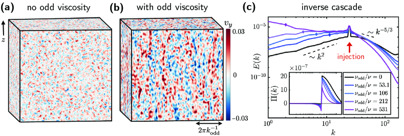
Figure 5: Wavelength selection in numerical inverse cascade. (a-b) Visualizations of the in-plane velocity $v_{y}$. In the absence of odd viscosity (a), structures of all scales are present, but are dominated by the injection scale. With odd viscosity $\nu_{\text{odd}}/\nu=212$ (b), secondary features appear on the scale of $\sim k_{\text{odd}}^{-1}$. The mechanism for this wavelength selection is the arrest of an inverse cascade, which can be observed if energy is injected at large wavenumbers (c). In this case, energy flows to large scales (inset), until it approaches the odd viscosity scale $k_{\text{odd}}$ (diamonds) where it is gradually arrested and leads to intermediate scale condensation. If $k_{\text{odd}}^{-1}$ is close to system size, energy sharply collects into largest available system-scale mode, as shown in Fig. 2f,g.

Navier-Stokes equation with odd viscosity

In an incompressible fluid, any gradient term in the Navier-Stokes equation can be absorbed in the pressure, without modifying the flow. Although a cylindrically symmetric viscosity tensor can have eight independent non-dissipative (odd) viscosities, the Navier-Stokes equation only contains two independent odd viscosity terms:

$$\rho_{0}D_{t}\bm{v} =-\nabla P+\eta\Delta\bm{v}$$ (16)

$$+\eta_{1}^{o}\begin{bmatrix}(\partial_{x}^{2}+\partial_{y}^{2})v_{y}\\ \\ -(\partial_{x}^{2}+\partial_{y}^{2})v_{x}\\ \\ 0\end{bmatrix}+\eta_{2}^{o}\begin{bmatrix}-\partial_{z}^{2}v_{y}-\partial_{y}\partial_{z}v_{z}\\ \\ \partial_{z}^{2}v_{x}+\partial_{x}\partial_{z}v_{z}\\ \\ \partial_{z}(\partial_{y}v_{x}-\partial_{x}v_{y})\end{bmatrix}$$

The forces due to the remaining odd viscosity coefficients can be expressed as linear combinations of the $\eta_{1}^{o}$ and $\eta_{2}^{o}$ terms and gradients of functions (see [23] for further details). In the main text, we consider the limit $\eta_{1}^{o}=-2\eta_{2}^{o}$, where we define $\eta_{\text{odd}}\equiv\eta_{2}^{o}$. In this case, the force due to the odd viscosities is $\eta_{\text{odd}}(\bm{e}_{z}\times\Delta\bm{v}-\nabla\omega_{z})$, where the second (gradient) term can be absorbed into the pressure.

Modified Taylor-Proudman theorem

The Taylor-Proudman theorem applied to a fluid under rotation implies $\partial_{z}\bm{v}=0$. In the main text, we have used an extension of this result to the case of a fluid with non-dissipative viscosities. Here, we give the detailed proof of this result for all non-dissipative viscosities compatible with cylindrical symmetry.

We first rewrite the odd force terms in the Navier-Stokes equation (Eq. 16) in terms of a cross product with $\bm{e}_{z}$:

$$\eta_{1}^{o}\begin{bmatrix}(\partial_{x}^{2}+\partial_{y}^{2})v_{y}\\ \\ -(\partial_{x}^{2}+\partial_{y}^{2})v_{x}\\ \\ 0\end{bmatrix}=-\eta_{1}^{o}\bm{e}_{z}\times\Delta_{\perp}\bm{v},$$ (17)

$$\eta_{2}^{o}\begin{bmatrix}-\partial_{z}^{2}v_{y}-\partial_{y}\partial_{z}v_{z}\\ \\ \partial_{z}^{2}v_{x}+\partial_{x}\partial_{z}v_{z}\\ \\ \partial_{z}(\partial_{y}v_{x}-\partial_{x}v_{y})\end{bmatrix}+\nabla\omega_{z}=\eta_{2}^{o}\bm{e}_{z}\times(\Delta\bm{v}-2\Delta_{\perp}\bm{v}),$$ (18)

where $\Delta_{\perp}\equiv\partial_{x}^{2}+\partial_{y}^{2}$. Note that we can add gradient terms to these expressions without modifying the flow. Assuming that the dominant balance is between the odd viscosity term and the pressure gradient term, we write for $\eta_{1}^{o}$:

$$-\eta_{1}^{o}\bm{e}_{z}\times\Delta_{\perp}\bm{v} =\nabla P.$$ (19)

Next, we take the curl of this equation to remove the pressure term, and simplify the resulting expression by applying the vector calculus identity

$$\bm{\nabla}\times(\bm{A}\times\bm{B})=\bm{A}(\bm{\nabla}\cdot\bm{B})-(\bm{A}\cdot\bm{\nabla})\bm{B}+(\bm{B}\cdot\bm{\nabla})\bm{A}-\bm{B}(\bm{\nabla}\cdot\bm{A}).$$

Enforcing incompressibility ($\nabla\cdot\bm{v}=0$), we obtain

$$\eta_{1}^{o}(\bm{e}_{z}\cdot\nabla)\Delta_{\perp}\bm{v} =0,$$ (20)

which can be simplified into a modified version of the Taylor-Proudman theorem:

$$\partial_{z}\Delta_{\perp}\bm{v} =0.$$ (21)

Repeating for $\eta_{2}^{o}$, we obtain

$$\partial_{z}(\Delta-2\Delta_{\perp})\bm{v} =0.$$ (22)

In the main text, we consider the simplifying limit $\eta_{1}^{o}=-2\eta_{2}^{o}$, in which case the theorem takes the form

$$\partial_{z}\Delta\bm{v} =0.$$ (23)

In an incompressible flow, all the odd viscosity coefficients compatible with cylindrical symmetry can be expressed as combinations of $\eta_{1}^{o}$ and $\eta_{2}^{o}$ (plus gradient terms that can be absorbed into the pressure). As the (modified) Taylor-Proudman theorem relies on the linearized Navier-Stokes equation (i.e., the Stokes equation), we can take linear combinations of Eqs. 20-21 above. Therefore, modified versions of the Taylor-Proudman theorem hold for all odd viscosities compatible with cylindrical symmetry.

Linear stability of the fluid and odd waves

To analyze the linear stability of a fluid with odd viscosity, we linearize the Navier-Stokes equations (1) about $\rho=\rho_{0}$ and $\bm{v}=\bm{0}$. We end up with the incompressible Stokes equations

$$\rho_{0}\partial_{t}v_{i} =-\partial_{i}P+\eta_{ijk\ell}\partial_{j}\partial_{\ell}v_{k}$$ (24)

$$\partial_{i}v_{i} =0.$$ (25)

Considering solutions of the form $\text{e}^{st+\text{i}\bm{k}\cdot\bm{x}}$, where $s=\sigma+\text{i}\omega$ is a complex growth rate, we rewrite them in Fourier space:

$$s\rho_{0}v_{i} =-ik_{i}P-\eta_{ijk\ell}k_{j}k_{\ell}v_{k}$$ (26)

$$k_{i}v_{i} =0.$$ (27)

Using the incompressibility condition, we solve for the pressure by multiplying by $k_{i}$, and find

$$P =i\eta_{ijk\ell}\frac{k_{i}k_{j}k_{\ell}}{k^{2}}v_{k}$$ (28)

Plugging this back into the Stokes equation, we arrive at an equation just for the velocity:

$$\rho_{0}sv_{n}=\eta_{ijk\ell}\frac{k_{n}k_{i}k_{j}k_{\ell}}{k^{2}}v_{k}-\eta_{njk\ell}k_{j}k_{\ell}v_{k}\equiv M_{nk}(\bm{k})v_{k}.$$ (29)

The dispersion relation $s(\bm{k})=\sigma(\bm{k})+\text{i}\omega(\bm{k})$ is then given by the eigenvalues of $iM_{nk}/\rho_{0}$.

In the case of Eq. (16) where the two independent odd viscosities $\eta_{1}^{o}$ and $\eta_{2}^{o}$ are present in addition to the normal shear viscosity $\eta$, we obtain

$$\rho_{0}\omega(\bm{k})=\pm\eta_{1}^{o}\frac{k_{z}(k_{x}^{2}+k_{y}^{2})}{|k|}\pm\eta_{2}^{o}\frac{k_{z}\mathinner{\!\left\lvert k_{x}^{2}+k_{y}^{2}-k_{z}^{2}\right\rvert}}{|k|}$$ (30)

in which the two $\pm$ are independent, and

$$\rho_{0}\sigma(\bm{k})=-\eta k^{2}.$$ (31)

In the main text, we consider the case $\eta_{1}^{o}=-2\eta_{2}^{o}$, in which case the above dispersion relations reduce to Eq. (7).

Details on the scaling arguments

The phenomenological theory of [45] relies on the following hypotheses: (i) energy is conserved away from injection and dissipative scales, (ii) the cascade is local, which means that different length scales are only coupled locally (e.g. very large scales are not directly coupled to very small scales), and (iii) the rate of energy transfer $\varepsilon(k)$ from scales higher than $k$ to scales smaller than $k$ is directly proportional to the triad correlation time $\tau_{3}$. Because of hypotheses (i) and (ii), rate of energy transfer $\varepsilon(k)$ is constant across the scales (i.e. does not depend on $k$), and can be identified with the energy dissipation rate $\epsilon$. In addition, because of hypothesis (ii), $\varepsilon(k)$ should only depend on local quantities $k$ and $E(k)$, in addition to $\tau_{3}(k)$. Therefore, using hypothesis (iii), we write

$$\epsilon=\varepsilon(k)=A\tau_{3}(k)k^{\alpha}E^{\beta}$$ (32)

where $A$ is a constant. The exponents are found using dimensional analysis (with $[E]=L^{3}T^{-2}$, $[\epsilon]=L^{2}T^{-3}$, $[k]=L^{-1}$, $[\tau_{3}]=T$), which yields $\alpha=4$ and $\beta=2$.

Scaling relation for $k_{\text{c}}$

For the condensation of the forward energy flux, the collapse of numerical results suggest that it can be described by a master scaling law

$$\frac{E(k)}{E_{0}(k)}\sim\begin{cases}1\quad&\text{for}\quad k\ll k_{\text{odd}},\\ \left(k/k_{\text{odd}}\right)^{s}\quad&\text{for}\quad k\gg k_{\text{odd}},\end{cases}$$ (33)

where we find $s=2/3$. Using the Kolmogorov spectrum for the case without odd viscosity, $E_{0}(k)\sim\epsilon^{2/3}k^{-5/3}$, we find for the energy spectrum

$$E(k)\sim\begin{cases}\epsilon^{2/3}k^{-5/3}\quad&\text{for}\quad k\ll k_{\text{odd}},\\ \epsilon^{2/3}k^{-5/3}\left(k/k_{\text{odd}}\right)^{s}\quad&\text{for}\quad k\gg k_{\text{odd}}.\end{cases}$$ (34)

This scaling continues until dissipation saturates the condensation. We can thus compute the condensation peak $k_{\text{c}}$ from the balance between injection and dissipation. Neglecting contributions to the dissipation from wavenumbers $k<k_{\text{odd}}$ and assuming $k_{\text{odd}}\ll k_{\text{c}}$, we obtain

$$\epsilon\sim\int_{0}^{k_{\text{c}}}\eta k^{2}E(k)dk,$$ (35)

yielding

$$\epsilon\sim\epsilon^{2/3}\eta k_{\text{c}}^{4/3}\left(k_{\text{c}}/k_{\text{odd}}\right)^{s},$$ (36)

resulting in the scaling relation for the peak condensation

$$k_{\text{c}}\sim(\epsilon^{1/3}\nu^{-1}k_{\text{odd}}^{s})^{\frac{1}{4/3+s}}\sim(k_{\nu}^{4/3}k_{\text{odd}}^{s})^{\frac{1}{4/3+s}},$$ (37)

where in the last relation, we substituted the normal Kolmogorov wavenumber $k_{\nu}\sim\epsilon^{1/4}\nu^{-3/4}$.

For $s=2/3$, we find

$$k_{\text{c}}\sim(k_{\nu}^{4/3}k_{\text{odd}}^{2/3})^{1/2}\sim\epsilon^{1/4}\nu^{-1/2}\nu_{\text{odd}}^{-1/4}.$$ (38)

Anisotropic spectra

Here, we consider the cylindrically-averaged spectra $E(k_{\perp},k_{z})$. These obey the cylindrical symmetry of the system, but being a function of two wavenumbers, they are not as straightforward to interpret as the spherically-averaged spectra $E(k)$ considered in the main text. Example spectra are shown in Fig. 6. The comparison of panels a and b (or panels c and d) evidences the two-dimensionalization in spectral space as gradual suppression of the modes with $k_{z}>0$.

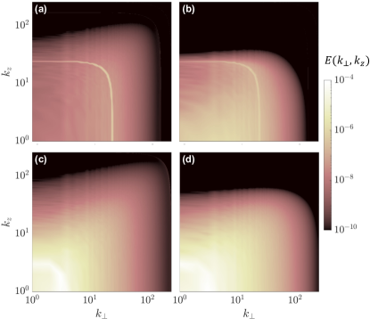
Figure 6: Anisotropic energy spectra. (a, b) Examples of $E(k_{\perp},k_{z})$ for the inverse cascading case ($k_{\text{in}}>k_{\text{odd}}$); without odd viscosity $\nu_{\text{odd}}=0$ (a) and with odd viscosity $\nu_{\text{odd}}=212\nu$ (b). (c,d) Examples of $E(k_{\perp},k_{z})$ for the direct cascading case ($k_{\text{in}}<k_{\text{odd}}$); without odd viscosity $\nu_{\text{odd}}=0$ (c) and with odd viscosity $\nu_{\text{odd}}=255\nu$ (d). This shows the two-dimensionalization effect of odd viscosity as gradual suppression of the modes with $k_{z}>0$.

Odd hyperviscosity

The crucial ingredient to observe this turbulent pattern formation is the competing direct cascade (at small $k$) and inverse cascade (at large $k$), and a non-dissipative mechanism that discriminates between the two. In fact, the scaling theories presented in this work can be straightforwardly extended to odd hyperviscosities of the form $\tilde{\eta}_{\text{odd}}\bm{e}_{z}\times\Delta^{p}\bm{v}$ with power $p>1$, which would make the transition from 3D to quasi-2D arbitrarily sharp/smooth, rendering also the region of spectral condensation arbitrarily peaked. This could be an ideal model system to study more complex natural geophysical or astrophysical flow systems in which a variety of different multi-scale mechanisms could exists that produce competing cascades, with either sharp or smooth transitions between them.

References

- Cardy et al. [2008] J. Cardy, G. Falkovich, K. Gawędzki, S. Nazarenko, and O. Zaboronski, Non-equilibrium Statistical Mechanics and Turbulence, London Mathematical Society Lecture Note Series (Cambridge University Press, 2008).
- Davidson [2015] P. Davidson, Turbulence: An Introduction for Scientists and Engineers (Oxford University Press, 2015).
- Falkovich et al. [2001] G. Falkovich, K. Gawędzki, and M. Vergassola, Reviews of Modern Physics 73, 913 (2001).
- Alexakis and Biferale [2018] A. Alexakis and L. Biferale, Physics Reports 767, 1 (2018).
- Eyink and Sreenivasan [2006] G. L. Eyink and K. R. Sreenivasan, Reviews of Modern Physics 78, 87 (2006).
- Frisch and Kolmogorov [1995] U. Frisch and A. N. Kolmogorov, Turbulence: the legacy of AN Kolmogorov (Cambridge university press, 1995).
- Avron et al. [1995] J. E. Avron, R. Seiler, and P. G. Zograf, Physical Review Letters 75, 697–700 (1995).
- Hoyos and Son [2012] C. Hoyos and D. T. Son, Physical Review Letters 108, 066805 (2012).
- Read [2009] N. Read, Physical Review B 79, 045308 (2009).
- Berdyugin et al. [2019] A. I. Berdyugin, S. G. Xu, F. M. D. Pellegrino, R. K. Kumar, A. Principi, I. Torre, M. B. Shalom, T. Taniguchi, K. Watanabe, I. V. Grigorieva, M. Polini, A. K. Geim, and D. A. Bandurin, Science 364, 162–165 (2019).
- Chapman et al. [1990] S. Chapman, T. Cowling, D. Burnett, and C. Cercignani, The Mathematical Theory of Non-uniform Gases: An Account of the Kinetic Theory of Viscosity, Thermal Conduction and Diffusion in Gases, Cambridge Mathematical Library (Cambridge University Press, 1990).
- Lingam et al. [2020] M. Lingam, P. J. Morrison, and A. Wurm, Journal of Plasma Physics 86, 10.1017/s0022377820001038 (2020).
- Morrison et al. [1984] P. J. Morrison, I. L. Caldas, and H. Tasso, Zeitschrift für Naturforschung A 39, 1023–1027 (1984).
- Fruchart et al. [2023] M. Fruchart, C. Scheibner, and V. Vitelli, Annual Review of Condensed Matter Physics 14, 471 (2023).
- Cross and Hohenberg [1993] M. C. Cross and P. C. Hohenberg, Reviews of Modern Physics 65, 851–1112 (1993).
- Cross and Greenside [2009] M. Cross and H. Greenside, Pattern Formation and Dynamics in Nonequilibrium Systems (Cambridge University Press, 2009).
- Tuckerman et al. [2020] L. S. Tuckerman, M. Chantry, and D. Barkley, Annual Review of Fluid Mechanics 52, 343 (2020).
- Prigent et al. [2002] A. Prigent, G. Grégoire, H. Chaté, O. Dauchot, and W. van Saarloos, Physical Review Letters 89, 014501 (2002).
- Duguet et al. [2010] Y. Duguet, P. Schlatter, and D. S. Henningson, Journal of Fluid Mechanics 650, 119 (2010).
- Kashyap et al. [2022] P. V. Kashyap, Y. Duguet, and O. Dauchot, Physical Review Letters 129, 244501 (2022).
- Biferale et al. [2012] L. Biferale, S. Musacchio, and F. Toschi, Physical Review Letters 108, 164501 (2012).
- Słomka and Dunkel [2017] J. Słomka and J. Dunkel, Proceedings of the National Academy of Sciences 114, 2119 (2017).
- Khain et al. [2022] T. Khain, C. Scheibner, M. Fruchart, and V. Vitelli, Journal of Fluid Mechanics 934, A23 (2022).
- Ganeshan and Abanov [2017] S. Ganeshan and A. G. Abanov, Physical Review Fluids 2, 094101 (2017).
- Beenakker and McCourt [1970] J. J. M. Beenakker and F. R. McCourt, Annual Review of Physical Chemistry 21, 47 (1970).
- McCourt [1990] F. McCourt, Nonequilibrium phenomena in polyatomic gases (Clarendon Press Oxford University Press, Oxford New York, 1990).
- Soni et al. [2019] V. Soni, E. S. Bililign, S. Magkiriadou, S. Sacanna, D. Bartolo, M. J. Shelley, and W. T. M. Irvine, Nature Physics 15, 1188–1194 (2019).
- Nakagawa [1956] Y. Nakagawa, Journal of Physics of the Earth 4, 105–111 (1956).
- Vollhardt and Wolfle [2013] D. Vollhardt and P. Wolfle, The Superfluid Phases of Helium 3 (Dover Publications, 2013).
- Wiegmann and Abanov [2014] P. Wiegmann and A. G. Abanov, Physical Review Letters 113, 034501 (2014).
- Zhao et al. [2022] Z. Zhao, M. Yang, S. Komura, and R. Seto, Odd viscosity in chiral passive suspensions (2022), arXiv:2205.11881 .
- Banerjee et al. [2017] D. Banerjee, A. Souslov, A. G. Abanov, and V. Vitelli, Nature Communications 8, 1573 (2017).
- Han et al. [2021] M. Han, M. Fruchart, C. Scheibner, S. Vaikuntanathan, J. J. de Pablo, and V. Vitelli, Nature Physics 17, 1260–1269 (2021).
- Markovich and Lubensky [2021] T. Markovich and T. C. Lubensky, Physical Review Letters 127, 048001 (2021).
- Fruchart et al. [2022] M. Fruchart, M. Han, C. Scheibner, and V. Vitelli, The odd ideal gas: Hall viscosity and thermal conductivity from non-hermitian kinetic theory (2022), arXiv:2202.02037 .
- Denk et al. [2016] J. Denk, L. Huber, E. Reithmann, and E. Frey, Physical Review Letters 116, 178301 (2016).
- Liebchen and Levis [2017] B. Liebchen and D. Levis, Physical Review Letters 119, 058002 (2017).
- Taylor [1923] G. I. Taylor, Proceedings of the Royal Society of London 104, 213 (1923).
- Proudman [1916] J. Proudman, Proceedings of the Royal Society of London 92, 408 (1916).
- Biferale et al. [2016] L. Biferale, F. Bonaccorso, I. M. Mazzitelli, M. A. T. van Hinsberg, A. S. Lanotte, S. Musacchio, P. Perlekar, and F. Toschi, Physical Review X 6, 041036 (2016).
- Buzzicotti et al. [2018] M. Buzzicotti, H. Aluie, L. Biferale, and M. Linkmann, Physical Review Fluids 3, 034802 (2018).
- Smith and Waleffe [1999] L. M. Smith and F. Waleffe, Physics of Fluids 11, 1608 (1999).
- Zeman [1994] O. Zeman, Physics of Fluids 6, 3221 (1994).
- Mininni et al. [2012] P. D. Mininni, D. Rosenberg, and A. Pouquet, Journal of Fluid Mechanics 699, 263 (2012).
- Kraichnan [1965] R. H. Kraichnan, Physics of Fluids 8, 1385 (1965).
- Zhou [1995] Y. Zhou, Physics of Fluids 7, 2092 (1995).
- Mahalov and Zhou [1996] A. Mahalov and Y. Zhou, Physics of Fluids 8, 2138 (1996).
- Chakraborty and Bhattacharjee [2007] S. Chakraborty and J. K. Bhattacharjee, Physical Review E 76, 036304 (2007).
- Grzybowski et al. [2000] B. A. Grzybowski, H. A. Stone, and G. M. Whitesides, Nature 405, 1033–1036 (2000).
- Yan et al. [2015] J. Yan, S. C. Bae, and S. Granick, Soft Matter 11, 147 (2015).
- Bililign et al. [2021] E. S. Bililign, F. Balboa Usabiaga, Y. A. Ganan, A. Poncet, V. Soni, S. Magkiriadou, M. J. Shelley, D. Bartolo, and W. T. M. Irvine, Nature Physics , 212–218 (2021).
- Tan et al. [2022] T. H. Tan, A. Mietke, J. Li, Y. Chen, H. Higinbotham, P. J. Foster, S. Gokhale, J. Dunkel, and N. Fakhri, Nature 607, 287–293 (2022).
- Dunkel et al. [2013] J. Dunkel, S. Heidenreich, K. Drescher, H. H. Wensink, M. Bär, and R. E. Goldstein, Physical Review Letters 110, 228102 (2013).
- Petroff et al. [2015] A. P. Petroff, X.-L. Wu, and A. Libchaber, Physical Review Letters 114, 158102 (2015).
- Wensink et al. [2012] H. H. Wensink, J. Dunkel, S. Heidenreich, K. Drescher, R. E. Goldstein, H. Löwen, and J. M. Yeomans, Proceedings of the National Academy of Sciences 109, 14308 (2012).
- Alert et al. [2022] R. Alert, J. Casademunt, and J.-F. Joanny, Annual Review of Condensed Matter Physics 13, 143 (2022).
- Martínez-Prat et al. [2019] B. Martínez-Prat, J. Ignés-Mullol, J. Casademunt, and F. Sagués, Nature Physics 15, 362 (2019).
- Squire et al. [2022] J. Squire, R. Meyrand, M. W. Kunz, L. Arzamasskiy, A. A. Schekochihin, and E. Quataert, Nature Astronomy 6, 715 (2022).
- Meyrand et al. [2021] R. Meyrand, J. Squire, A. Schekochihin, and W. Dorland, Journal of Plasma Physics 87, 535870301 (2021).
- Miloshevich et al. [2021] G. Miloshevich, D. Laveder, T. Passot, and P. L. Sulem, Journal of Plasma Physics 87, 905870201 (2021).
- Diamond et al. [2005] P. H. Diamond, S.-I. Itoh, K. Itoh, and T. S. Hahm, Plasma Physics and Controlled Fusion 47, R35 (2005).
- Sukoriansky et al. [2007] S. Sukoriansky, N. Dikovskaya, and B. Galperin, Journal of the Atmospheric Sciences 64, 3312 (2007).
- Berloff et al. [2009] P. Berloff, I. Kamenkovich, and J. Pedlosky, Journal of Fluid Mechanics 628, 395 (2009).
- Chekhlov et al. [1996] A. Chekhlov, S. A. Orszag, S. Sukoriansky, B. Galperin, and I. Staroselsky, Physica D: Nonlinear Phenomena 98, 321 (1996).
- Rhines [1975] P. B. Rhines, Journal of Fluid Mechanics 69, 417 (1975).
- Rhines [1979] P. B. Rhines, Annual Review of Fluid Mechanics 11, 401 (1979).
- Legras et al. [1999] B. Legras, B. Villone, and U. Frisch, Physical Review Letters 82, 4440 (1999).
- Grianik et al. [2004] N. Grianik, I. M. Held, K. S. Smith, and G. K. Vallis, Physics of Fluids 16, 73 (2004).
- Falkovich [1994] G. Falkovich, Physics of Fluids 6, 1411 (1994).
- Küchler et al. [2019] C. Küchler, G. Bewley, and E. Bodenschatz, Journal of Statistical Physics 175, 617 (2019).
- Lohse and Müller-Groeling [1995] D. Lohse and A. Müller-Groeling, Physical Review Letters 74, 1747 (1995).
- Donzis and Sreenivasan [2010] D. A. Donzis and K. R. Sreenivasan, Journal of Fluid Mechanics 657, 171 (2010).
- Verma and Donzis [2007] M. K. Verma and D. Donzis, Journal of Physics A: Mathematical and Theoretical 40, 4401 (2007).
- Sreenivasan and Antonia [1997] K. R. Sreenivasan and R. A. Antonia, Annual Review of Fluid Mechanics 29, 435 (1997).
- Kolmogorov [1941] A. N. Kolmogorov, in Dokl. Akad. Nauk SSSR, Vol. 31 (1941) p. 99.
- Connaughton et al. [2004] C. Connaughton, R. Rajesh, and O. Zaboronski, Physical Review E 69, 10.1103/physreve.69.061114 (2004).
- Cheng and Redner [1988] Z. Cheng and S. Redner, Physical Review Letters 60, 2450 (1988).
- Politi and Misbah [2006] P. Politi and C. Misbah, Physical Review E 73, 036133 (2006).
- Politi and Misbah [2004] P. Politi and C. Misbah, Physical Review Letters 92, 090601 (2004).
- Halatek and Frey [2018] J. Halatek and E. Frey, Nature Physics 14, 507 (2018).
- Brauns et al. [2021] F. Brauns, H. Weyer, J. Halatek, J. Yoon, and E. Frey, Physical Review Letters 126, 104101 (2021).
- Cates and Tailleur [2015] M. E. Cates and J. Tailleur, Annual Review of Condensed Matter Physics 6, 219 (2015).