Measuring the Hubble Constant Using Strongly Lensed Gravitational Wave Signals

Abstract

The measurement of the Hubble constant $H_{0}$ plays an important role in the study of cosmology. In this work, we propose a new method to constrain the Hubble constant using the strongly lensed gravitational wave (SLGW) signals. Through reparameterization, we find that the lensed waveform is sensitive to the $H_{0}$. Assuming the scenario that no electromagnetic counterpart of the GW source can be identified, our method can still give meaningful constraints on the $H_{0}$ with the information of the lens redshift. We then apply Fisher information matrix and Markov Chain Monte Carlo to evaluate the potential of this method. For the space-based GW detector, TianQin, the $H_{0}$ can be constrained within a relative error of $\sim$ 1% with a single SLGW event.

I Introduction

The Hubble constant has been independently measured by various methods with ever-increasing measurement precision in recent years. However, type-Ia supernovae (SNe Ia) observations consistently prefer a higher value of $H_{0}=73.04\pm 1.04\mathrm{\ km\ s^{-1}\ Mpc^{-1}}$ Riess et al. (2022), while the cosmic microwave background (CMB) observations prefer a lower value of $H_{0}=67.4\pm 0.5\mathrm{\ km\ s^{-1}\ Mpc^{-1}}$ under the flat $\Lambda$ cold dark matter ($\Lambda$CDM) model Planck Collaboration et al. (2020). The discrepancy between these two reference measurements is thus established at 5$\sigma$, which is recognized as the “Hubble crisis” Di Valentino et al. (2021); Riess et al. (2022).

Ever since the first direct detection in September 2015, 90 gravitational wave (GW) events have been reported by the LIGO-Virgo-KAGRA (LVK) collaboration Abbott et al. (2019, 2021a, 2021b, 2021c, 2021d), which made the GW observation a new window to understanding the Universe. GW signals provide direct measurements of the luminosity distance, and combined with the redshift information, they can serve as standard sirens to map the evolution of the Universe Schutz (1986); Holz and Hughes (2005); Nissanke et al. (2013); Abbott et al. (2017). The latest LVK measurement yields $H_{0}=68^{+8}_{-6}\mathrm{\ km\ s^{-1}\ Mpc^{-1}}$ using 47 GW events from the third LVK Gravitational-Wave Transient Catalog (GWTC–3) Abbott et al. (2021e).

If the GW from a coalescing binary passes near massive objects, gravitational lensing (GL) will affect the GW in the same way as it does for light Wang et al. (1996); Nakamura (1998); Takahashi and Nakamura (2003), which will influence the strain of GW, and, in strong lensing cases, produce multiple images with arrival time delay. It has been proposed that the GL can also be used to study cosmology by measuring the difference in arrival time from multiple images and some lens properties Refsdal (1964); Treu (2010). This idea has been applied in the electromagnetic (EM) domain to infer the value of $H_{0}=73.3^{+1.7}_{-1.8}\mathrm{\ km\ s^{-1}\ Mpc^{-1}}$ from a joint analysis of six lensed quasars in flat $\Lambda$CDM Treu and Marshall (2016); Wong et al. (2020). Several searches for GW lensing signatures have already been performed during the first three observing (from O1 to O3) runs (see Hannuksela et al. (2019); The LIGO Scientific Collaboration et al. (2021); Diego et al. (2021) and the references therein), and there is still no officially confirmed lensing signal by LVK. The lensed GW signals are also expected to be detected by space-based gravitational wave detectors such as LISA Amaro-Seoane et al. (2017); Gao et al. (2022).

Recently it’s been realized that time delays between multiple signals of lensed GWs by the future GW detections can be used to measure the Hubble constant Sereno et al. (2011); Liao et al. (2017); Wei and Wu (2017); Li et al. (2019); Cremonese and Salzano (2020); Hannuksela et al. (2020); Cao et al. (2022); Hou et al. (2021); Qi et al. (2022). Liao et al. Liao et al. (2017) reported a waveform-independent strategy by combining the accurately measured time delays from strongly lensed gravitational wave (SLGW) signals with the images and lens properties observed in the EM domain and shows that 10 such systems are sufficient to constrain the Hubble constant within an uncertainty of $0.68\%$ for a flat $\Lambda$CDM universe in the era of third-generation ground-based detectors.

The traditional GW cosmology method relies on the identification of the EM counterpart or the host galaxy of the GW source Schutz (1986), which may not always be feasible. In this work, we propose a new method to measure the Hubble constant $H_{0}$ using SLGW signals. The waveform is reparameterized to explicitly include $H_{0}$ in the parameter set. We find that the SLGW waveforms are sensitive to $H_{0}$, making the system a promising probe to study the Universe even without the identification of the EM counterpart of the GW source. This was made possible by utilizing the waveform per se, instead of just the time delay or the magnification Sereno et al. (2011); Liao et al. (2017); Wei and Wu (2017); Li et al. (2019); Cremonese and Salzano (2020); Hannuksela et al. (2020); Cao et al. (2022); Hou et al. (2021); Qi et al. (2022). The method we propose here only requires the SLGW signal and the lens redshift. Since the lenses are closer, they might be easier to observe compared to GW sources. As a result, our method is capable of measuring $H_{0}$ even when the host galaxy is too dark to be directly observable.

We evaluate the potential of this new method in measuring the Hubble constant and provide preliminary results for TianQin, which is a planned space-based GW observatory sensitive to the millihertz band Luo and others (TianQin Collaboration). In recent years, a significant amount of effort has been put into the study and consolidation of the science cases for TianQin Hu et al. (2017); Wang et al. (2019); Feng et al. (2019); Bao et al. (2019); Shi et al. (2019); Liu et al. (2020); Fan et al. (2020); Huang et al. (2020); Mei and others (TianQin Collaboration); Zi et al. (2021); Liang et al. (2022); Liu et al. (2022); Zhu et al. (2022a, b); Zhang et al. (2022); Lu et al. (2022); Sun et al. (2022); Xie et al. (2022). For the detected GW sources, TianQin’s sky localization precision can reach the level of 1 deg² to 0.1 deg² Wang et al. (2019); Liu et al. (2020); Fan et al. (2020); Huang et al. (2020), which makes it possible to combine subsequent EM observations to implement multi-messenger astronomy. For an order-of-magnitude estimation of the SLGW detection rate, we adopt the detecting probability of SLGW from massive binary black hole (MBBH) mergers as $\sim 1\%$ for space-based gravitational wave detector Gao et al. (2022), while under the optimistic model, the detection rate of GW from MBBH is $\gtrsim O(10^{2})/yr$ Wang et al. (2019). Therefore the total detection number for SLGW events can be as high as $\gtrsim O(5)$ over the five-year mission lifetime. We consider three cases: a) lens only, b) GW source only, and c) GW source and lens simultaneously. These cases represent different levels of information available, in the last two we assume the optimistic case where the EM counterpart of GW source is observed. This can be justified as some studies have argued that if the massive binary black hole evolve in gas-rich environment, the accretion of gas could produce EM radiation d’Ascoli et al. (2018), which can be used to determine the source redshift Tamanini et al. (2016). Our calculations show that the Hubble constant can be well constrained using our method in all three cases, even in the absence of the GW source’s EM counterpart.

This manuscript is organized as follows. In section II, we describe our method to measure $H_{0}$ using SLGW signals. In section IV, we evaluate the expected measurement precision of H0 using our new method. Finally, we summarize and discuss in section V. Throughout this manuscript, we use $G=c=1$ and assume a flat $\Lambda$CDM cosmology with the parameters $\Omega_{M}=0.315$, $\Omega_{\Lambda}=0.685$. For the simulation, we also adopt $H_{0}=67.66\mathrm{\ km\ s^{-1}\ Mpc^{-1}}$ Planck Collaboration et al. (2020).

II The SLGW signals

The strong GL not only alters the GW amplitude and phase but also produces multiple duplicates of the same signal. The calculation of the SLGW waveform considering the detector response is complicated and generally speaking, there is no compact form. However, analytical description is available when certain simplifications are adopted. For example, in the case of the point mass (PM) lens model, and utilizing the geometric optics approximation (which means that the Schwarzschild radius of the lens is much larger than the wavelength of the GWs), one can express the waveform as a superposition of two GW signals. This can be derived by applying the stationary phase approximation, which is valid as the GWs phases evolve much faster than their amplitude. One can derive Takahashi and Nakamura (2003)

$${\widetilde{h}}_{\alpha}^{L}\left(f\right) = \bigg{[}|\mu_{+}|^{1/2}\Lambda_{\alpha}(t)e^{-i(\phi_{D}+\phi_{p,\alpha})(t)}$$ (1)

$$-i|\mu_{-}|^{1/2}e^{2\pi ift_{d}}\Lambda_{\alpha}(t+t_{d})e^{-i(\phi_{D}+\phi_{p,\alpha})(t+t_{d})}\bigg{]}$$

$$\times\mathcal{A}f^{-7/6}e^{i\Psi(f)},\qquad\qquad\qquad\alpha=I,II$$

where $\alpha=I,II$ denotes the index of two interferometer. In this proof-of-principle study, for the convenience and efficiency of calculation, we use this analytical waveform derived from the point-mass model and geometric optics approximation to simulate the SLGW signals. The GW amplitude and phase are

$$\mathcal{A}=\sqrt{\frac{5}{96}}\frac{\pi^{-2/3}\mathcal{M}_{z}^{5/6}}{D_{S}(1+z_{S})^{2}}$$ (2)

and

$$\Psi(f)=2\pi ft_{\mathrm{c}}-\phi_{\mathrm{c}}-\frac{\pi}{4}+\psi_{\mathrm{PN}},$$ (3)

where $D_{S}$ is the angular diameter distances from the source to the observer, $D_{S}(1+z_{S})^{2}$ is the luminosity distance to the source, and $\psi_{\mathrm{PN}}$ is the post-Newtonian (PN) phase as a function of the redshifted chirp mass $\mathcal{M}_{z}=(1+z_{S})(M_{1}M_{2})^{3/5}/(M_{1}+M_{2})^{1/5}$ and symmetric mass ratio $\eta=(M_{1}M_{2})/(M_{1}+M_{2})^{2}$. In this work, we expand the PN phase to 2 PN order (see Feng et al. (2019) and the references therein).

The initial frequency of the waveform is

$$f_{\mathrm{in}}=(5/256)^{3/8}\frac{1}{\pi}\mathcal{M}_{z}^{-5/8}(t_{c}-t)^{-3/8},$$ (4)

and we adopt the cutoff frequency at the innermost stable circular orbit (ISCO)

$$f_{\mathrm{ISCO}}=(6^{3/2}\pi M_{z})^{-1},$$ (5)

where $M_{z}=(1+z_{S})(M_{1}+M_{2})$ is the redshifted total mass.

The detector response, the polarization phase, and the Doppler phase can be defined by

$$\Lambda_{\alpha}(t) = \sqrt{(1+\cos^{2}\iota)^{2}{F_{\alpha}^{+}(t)}^{2}+4\cos^{2}\iota{F_{\alpha}^{\times}(t)}^{2}},$$ (6)

$$\phi_{P,\alpha}(t) = {\tan}^{-1}\ \left[\frac{{2\cos\iota\ F}_{\alpha}^{\times}(t)}{{(1+\cos^{2}\iota)F}_{\alpha}^{+}(t)}\right],$$ (7)

and

$$\phi_{D}(t)=2\pi fR\sin\left(\frac{\pi}{2}-\beta\right)\ \cos(2\pi f_{\mathrm{m}}t-\lambda),$$ (8)

with $R=1$ AU and $f_{m}=1/\mathrm{year}$. $F_{\alpha}^{+,\times}(t)$ is the antenna pattern functions of the source position ($\beta,\lambda$) and polarization angle $\psi_{S}$ Huang et al. (2020), and related to the motion and pointing of the detector.

The magnification factor of each image and the time delay between the double images for the case of the PM lens are given by Takahashi and Nakamura (2003)

$$\mu_{\pm}=\frac{1}{2}\pm\frac{y^{2}+2}{2y\sqrt{y^{2}+4}}$$ (9)

and

$$t_{d} = 4M_{L}(1+z_{L})\left[\frac{y\sqrt{y^{2}+4}}{2}+\ln\left(\frac{\sqrt{y^{2}+4}+y}{\sqrt{y^{2}+4}-y}\right)\right],$$

where $y=D_{L}\eta_{L}/(D_{S}\xi_{0})$ is the dimensionless source position in the lens plane, $D_{L}$ is the angular diameter distances from the lens to the observer, $\eta_{L}$ and $\xi_{0}$ are the GW source position in the lens plane and the normalization constant of the length, respectively. When $y\rightarrow\infty$ ($\mu_{+}=1$ and $\mu_{-}=0$), Eq. (1) reduces to the unlensed waveform.

For the case of the PM lens, the normalization constant can be given by $\xi_{0}=\sqrt{4M_{L}D_{L}D_{LS}/D_{S}}$, where $D_{LS}$ is the angular diameter distances from the source to the lens, and $M_{L}$ is the lens mass. In this case, the dimensionless source position can be written as

$$y=\frac{\eta_{L}}{2\sqrt{M_{L}}}\sqrt{\frac{D_{L}}{D_{S}D_{LS}}},$$ (11)

using the distance-redshift relationship Hogg (1999)

$$D=\frac{1}{H_{0}(1+z)}\int_{0}^{z}dz^{\prime}\frac{1}{E(z^{\prime})},$$ (12)

where $E(z^{\prime})$ depicts the background evolution of the Universe, it can be found that $y$ is proportional to $\sqrt{H_{0}}$ in the PM lens model.

For the singular isothermal sphere (SIS) lens model, there are

$$\mu_{\pm}=\pm 1+\frac{1}{y}$$ (13)

and

$$t_{d} = 8M_{L}(1+z_{L})y,$$ (14)

where the lens mass inside the Einstein radius is given by $M_{L}=4\pi^{2}v_{d}^{4}D_{L}D_{LS}/D_{S}$, and $v_{d}$ is the velocity dispersion of lens galaxy. In this case, the dimensionless source position can be written as

$$y=\frac{\eta_{L}}{4\pi v_{d}^{2}D_{LS}}.$$ (15)

Using the distance-redshift relationship again, $y$ is proportional to $H_{0}$ in the SIS lens model.

For general GW signals with no EM counterpart, it is usually impossible to measure the Hubble constant since it degenerates with other parameters Schutz (1986). The SLGW signals provides a mechanism to measure the Hubble constant directly, as the GL effect carries the information of $D_{S}$ while the GW amplitude is linked with $D_{S}(1+z_{S})^{2}$. When the GL redshift is known, the GW source redshift can be determined. The cosmological information is embedded in the SLGW waveform, and therefore constraining $H_{0}$ becomes possible even if the EM counterpart is not available.

Assuming a flat $\Lambda$CDM model, we can describe a lensed waveform with a set of 13 parameters: the Hubble constant $H_{0}$, lens mass $M_{L}$, lens redshift $z_{L}$, GW source position in the lens plane $\eta_{L}$, GW source redshift $z_{S}$, redshifted chirp mass $\mathcal{M}_{z}$, symmetric mass ratio $\eta$, inclination angle $\iota$, coalescence time $t_{c}$, coalescence phase $\phi_{c}$, GW source ecliptic coordinates $\beta$, $\lambda$, and polarization angle $\psi_{S}$.

III Parameter Estimation Methods

To evaluate the potential of measuring the Hubble constant using the SLGW signals, we apply both analytical and numerical methods with Fisher information matrix (FIM) and Markov Chain Monte Carlo (MCMC), respectively.

The FIM $\Gamma_{ij}$ is defined as

$$\Gamma_{ij}=\left(\frac{\partial h}{\partial\theta_{i}}\bigg{|}\frac{\partial h}{\partial\theta_{j}}\right),$$ (16)

where $\theta_{i}$ stands for the $i$-th GW parameter, In the limit that a signal is associated with a large signal-to-noise ratio (SNR) $\rho=\sqrt{(h|h)}\gg 1$, one can approximate the variance-covariance matrix with the inverse of the FIM $\Sigma=\Gamma^{-1}$, with $\Sigma_{ii}$ describing the marginalized variances of the $i$-th parameter.

Under the framework of Bayesian inference, one would like to constrain parameters $\theta$ with data $d$, or to obtain the posterior distribution $p(\theta|d,H)$ under model $H$. Under the Bayes’ theorem,

$$p(\theta|d,H)=\frac{p(\theta|H)p(d|\theta,H)}{p(d|H)},$$ (17)

the posterior is the product of the prior $p(\theta|H)$ and the likelihood $p(d|\theta,H)$, normalized by the evidence $p(d|H)$. The likelihood of the GW signal can be written as

$$p(d|\theta,H)\propto\exp\left[-\frac{1}{2}\bigg{(}d-h(\theta)\bigg{|}d-h(\theta)\bigg{)}\right],$$ (18)

where the inner product $(\cdot|\cdot)$ defined as Finn (1992); Cutler and Flanagan (1994)

$$(a|b)=4\Re e\int^{\infty}_{0}\mathrm{d}f\frac{\tilde{a}^{*}(f)\tilde{b}(f)}{{S}_{n}(f)},$$ (19)

and $S_{n}(f)$ is the one-sided power spectral density, we adopt the formula from Huang et al. (2020) for the expression of TianQin. In our case we consider the SLGW waveform $h(\theta)$ described by Eq. (1). We adopt the emcee Foreman-Mackey et al. (2013) implementation of the affine invariant MCMC sampler.

IV Measurement precision of $H_{0}$

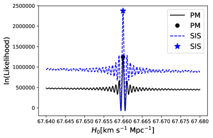
Figure 1: The conditional probability of $H_{0}$ for PM (black solid line) and SIS (blue dashed line) lens model, respectively, the black point and blue star indicates the injected value.

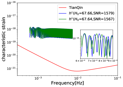
Figure 2: Two strongly lensed waveforms, with all other parameters fixed but $H_{0}$ slightly different. The values of parameters are listed at the beginning of Sec. IV

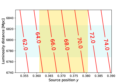
Figure 3: The contour of $H_{0}$ over different luminosity distances and source positions. The blue and yellow shaded regions represent the measurement error from FIM analysis around the true value, showing that measurement of both parameters can be used to constrain the Hubble constant.

For the lens system parameters, we choose the lens mass $M_{L}=1\times 10^{12}\,\mathrm{M}_{\odot}$, the lens redshift $z_{L}=0.5$, the GW source position $\eta_{L}=5$ kpc, and the GW source redshift $z_{S}=1$. For the remaining GW source parameters, we adopt the redshifted chirp mass $\mathcal{M}_{z}=2.43\times 10^{5}\,\mathrm{M}_{\odot}$, symmetric mass ratio $\eta=0.222$ ($M_{1}=2\times 10^{5}\,\mathrm{M}_{\odot}$, $M_{2}=1\times 10^{5}\,\mathrm{M}_{\odot}$), inclination angle $\iota=\pi/3$, coalescence time $t_{c}=2^{18}$ s ($\sim 3\ \mathrm{days}$), coalescence phase $\phi_{c}=\pi/2$, GW source ecliptic coordinates $\beta=-4.7^{\circ}$, $\lambda=120.4^{\circ}$ (The zenith of TianQin), and polarization angle $\psi_{S}=\pi/2$.

We first inject a simulated SLGW signal $h(H_{0}^{\rm inject})$ without noise, and match it with a signal with different Hubble constant $h(H_{0}^{\rm match})$. The log likelihood is calculated as $\left(h(H_{0}^{\rm inject})\middle|h(H_{0}^{\rm match})\right)-\frac{1}{2}\left(h(H_{0}^{\rm match})\middle|h(H_{0}^{\rm match})\right)$, In Figure 1 we demonstrate the sensitivity of log likelihood with respect to the Hubble constant for the PM (black solid line) and SIS (blue dashed line) lens model, respectively. It can be found that the sensitivity curves of PM and SIS models are similar in shape, except that the log likelihood function value of SIS model is larger because the magnification of GL effect is larger. For convenience, the PM model is used for subsequent calculations. We observe that the log likelihood varies violently at the level of $0.001\mathrm{\ km\ s^{-1}\ Mpc^{-1}}$, or $10^{-5}$ for relative uncertainty in Figure 1. The amplitude of the injected lensed waveform as well as a typical template is shown in Figure 2. We observe that indeed that the lensed waveform is highly sensitive to the choice of $H_{0}$ and even a tiny difference in the Hubble constant can lead to significant deviation in the waveform.

Given all other parameters fixed, Figure 1 and 2 indidcate that the waveform is highly sensitive to the Hubble constant. However, we do not know other parameters a priori, and due to the degeneracy between parameters, if neither lens redshift $z_{L}$ nor $z_{S}$ is determined, one can not constrain the Hubble constant. However, studies suggested that space-borne GW missions have the potential to accurately localize sources, especially when a network of detectors is considered (e.g. Gong et al., 2021; Liu et al., 2022). Therefore, it is fair to assume that although the EM counterpart might be absent, some EM information is still available to break the degeneracy. For the following analysis, we choose to fix the other cosmological parameter $\Omega_{M}$ as we specifically focus on the $H_{0}$. We also fix angles like $\beta,\ \lambda$, as any EM information about the lens or the host galaxy can help to set these angles Wong et al. (2020); Dye and Warren (2005); Schutz (1986); Bogdanović et al. (2022). We consider three cases for the different observed EM counterparts: a) lens only, in which case we fix $z_{L}$, b) GW source only, where we fix $z_{S}$, and c) GW source and lens simultaneously, where both $z_{L}$ and $z_{S}$ are fixed.

In Figure 3, we illustrate that by matching template with injected signal, one can constrain both the luminosity distance $D_{S}(1+z_{S})^{2}$ and the source location $y$, with the associated uncertainties represented by the shaded regions. From simple derivation one can deduce that by measuring both parameters, it is possible to constrain the Hubble constant. The FIM analysis predicts that the $H_{0}$ can be constrained to the relative precision to 2.01%, 0.42%, and 0.31%, for case a), b) and c) respectively.

We present an example posterior distribution in Figure 4 from the MCMC sampling, with the black contour lines indicating 90% credible region and we fix lens redshift $z_{L}$. We adopt the uniform prior for $H_{0}\in(40,100)\mathrm{\ km\ s^{-1}\ Mpc^{-1}}$, $\eta_{L}\in(0,10)$ kpc, $\eta\in(0,0.25)$, $\cos\iota\in(0,1)$, and $\phi_{c}\in(-\pi,\pi)$. For $M_{L}$, $\mathcal{M}_{z}$, $t_{c}$, and $z_{S}$, we adopt uniform priors greater than zero, with the constraint that $z_{S}\textgreater z_{L}$. We check the convergence of the MCMC by looking at the Gelman-Rubin statistic Gelman and Rubin (1992), and for all parameters they are consistently smaller than 1.05.

In Figure 4, we overlap the red ellipses as FIM 90% credible regions for comparison. It can be observed that the two methods give consistent results, both predict that even with many parameters unfixed, the lensing waveform method can still pinpoint the Hubble constant $H_{0}$ to the level of 1%. Notice that this value is about three orders of magnitude worse than from Figure 1. This can be explained by the large correlation between $H_{0}$ and other parameters like source redshift $z_{S}$ and lens mass $M_{L}$. Nevertheless, the 1% level precision of $H_{0}$ is still highly encouraging, as it provides an independent measurement from a single event, and it can be achieved even without the direct EM counterpart identification.

In addition, we add $\beta$ and $\lambda$ into the calculation of the FIM. The $H_{0}$ can be constrained to the relative precision to 4.34%, and the measurement accuracy of $\beta$ and $\lambda$ are 0.0044 rad and 0.0002 rad, respectively.

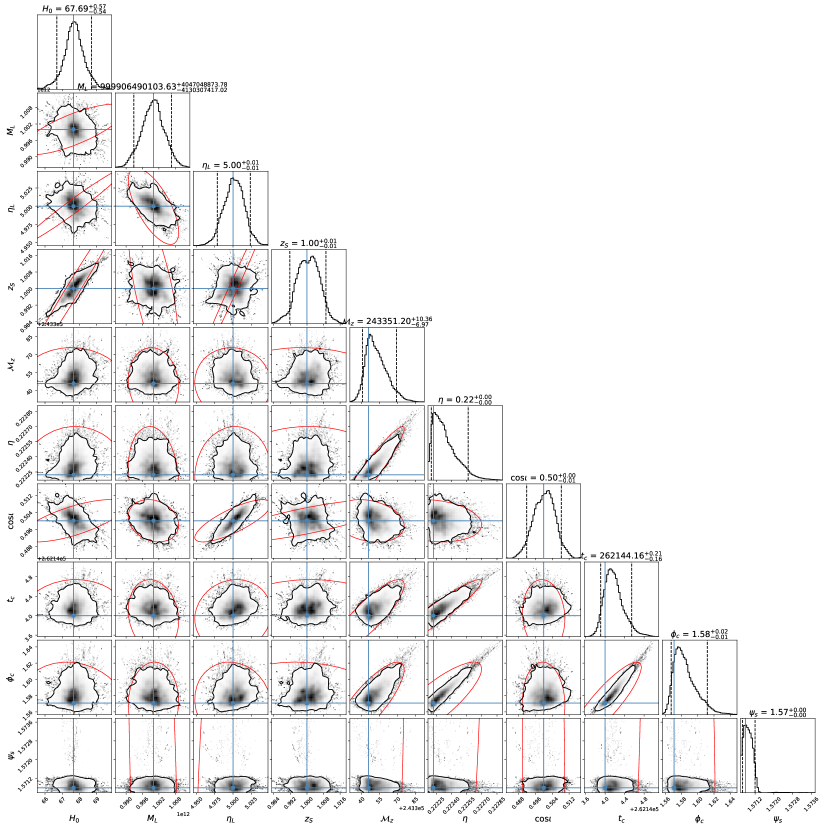
Figure 4: Comparison between the posterior distribution sampled by MCMC (black) and the ellipses based on the FIM (red) with 90% credible regions.

V Summary and discussion

In this work, we proposed a new method to measure the Hubble constant using SLGW signals. For such systems, the luminosity distance and the location parameter $y$ by the GW waveform and the GL pattern, respectively, which in principle can be used to constrain the Hubble constant. We reparameterize the waveform to include the Hubble constant in the parameter set. We find that the space-borne GW missions can determine the Hubble parameter to the relative precision of 1%, even when the EM counterpart or host galaxy is absent. In this method, we relax the requirement on the identification of the EM counterpart or host galaxy, as the cosmological information is already embedded within the lensed waveform (see Eq. (1), (2),(9)-(12)). So our work extract cosmological parameters from the waveform while many previous works only use information distilled from the waveform, like the time differences between images and magnification factors Sereno et al. (2011); Liao et al. (2017); Wei and Wu (2017); Li et al. (2019); Cremonese and Salzano (2020); Hannuksela et al. (2020); Cao et al. (2022); Hou et al. (2021); Qi et al. (2022). When the EM counterpart is identified and the source redshift $z_{S}$ is also fixed, one can constrain $H_{0}$ to the level of 0.3%.

We adopted a number of simplifications in this proof-of-principle study. For example, we only considered the PM lens model for lensing effect calculation. In future we can extend to more general models like the SIS or the Navarro-Frenk-White model. Secondly, we calculate the GL effect under the geometric optics approximation Takahashi and Nakamura (2003). For the parameters we choose it is still valid, but a more general treatment would require the consideration of wave optics Takahashi and Nakamura (2003); Gao et al. (2022). Last but not least, we only considered the PN waveform for the inspiral of a quasi-circular, non-spinning compact binary. Although this hugely saves the computation time, we plan to include a full inspiral-merger-ringdown waveform for a more general binary in the future for more realistic analysis. We remark though that the discard of merger and ringdown means that a portion of information and SNR are not used and we expect a better constraint with the consideration of the IMR waveforms.