Enhanced efficiency in quantum Otto engine via additional magnetic field
and effective negative temperature

Abstract

A four-stroke quantum Otto engine can outperform when conducted between two thermal reservoirs, one at a positive spin temperature and the other one at an effective negative spin temperature. Along with a magnetic field in the $(x,y)$-plane, we introduce an additional magnetic field in the $z$-direction. We demonstrate that the efficiency increases with the increase in the strength of the additional magnetic field although the impact is not monotonic. Specifically, we report a threshold value of the magnetic field, depending on the driving time which exhibits a gain in efficiency. We argue that this benefit may result from the system being more coherent with driving time, which we assess using the $l_{1}$-norm coherence measure. Moreover, we find that the increment obtained in efficiency with an additional magnetic field endures even in presence of disorder in parameter space.

I Introduction

The goal of a thermal machine is to maximize the work which is obtained from the conversion of heat through a reversible process Peña et al. (2020). For instance, they have been used to store energy like in batteries, to decrease the temperature in quantum refrigerators, and to produce motion, essential to manufacture vehicles. In the middle of last century, it was discovered that the efficiencies of thermal machines can be qualitatively improved if they are built using quantum systems having finite or infinite dimensions Scovil and Schulz-DuBois (1959); Jochen Gemmer (2009); Deffner and Campbell (2019); Myers et al. (2022). By exploiting atomic coherence, a quantum Carnot engine containing a heat bath of three-level atoms was found which can provide higher efficiency than that can be obtained by classical engine Scully et al. (2003, 2003). Heat engines have been studied with different reservoirs including squeezed Klaers et al. (2017); de Assis et al. (2021); Zhang (2020); Tabatabaei et al. (2022); Hardal et al. (2017); Scully (2001); Huang et al. (2012); Zagoskin et al. (2012); Roßnagel et al. (2014); Altintas et al. (2014); Long and Liu (2015); Xiao and Li (2018); Niedenzu et al. (2018); Wang et al. (2019); de Assis et al. (2020), spin  Wright et al. (2018), superconducting reservoirs Tabatabaei et al. (2022); Hardal et al. (2017), etc. Importantly, current technological advances promise to build such reservoirs in physical systems like trapped ions, cavity QED, nuclear magnetic resonance (NMR) etc Murch et al. (2013); Carvalho et al. (2001); Werlang et al. (2008); Pielawa et al. (2007); Werlang and Villas-Boas (2008); Prado et al. (2009); Verstraete et al. (2009); Hama et al. (2018); Lovrić et al. (2007); Álvarez and Suter (2011a). The main motive behind this quantum reservoir engineering is to find ways to obtain a better overall performance of the engines Myers et al. (2022); Mendonça et al. (2020). On the other hand, there are also constant efforts to quantify quantum correlations from the thermodynamic perspective Ollivier and Zurek (2001); Oppenheim et al. (2002); Horodecki et al. (2005); Bera et al. (2017) and such quantities can also be shown to have relation with the efficiency of quantum Carnot engines Dillenschneider and Lutz (2009); Perarnau-Llobet et al. (2015).

In the practical world, the Otto cycle is used in a spark-ignition engine, which is the type of engine commonly found in cars and small vehicles Breeze (2019). The Otto cycle was developed for a number of reasons, including great efficiency while emitting little emissions Heywood (2018); Hill and Peterson (1991); Stone (1985), and has applications ranging from small generators to massive industrial engines. In a similar spirit, it was realized that the quantum version of the Otto engine (QOE) consists of four strokes – in two of the strokes, a working medium is connected to cold or hot thermal reservoirs while the working medium either expands or compresses unitarily, thereby producing work in the other two strokes. In this work, we will be concentrating on two thermal reservoirs, one at a positive temperature while the other one is prepared at an effective negative temperature de Assis et al. (2019); Nettersheim et al. (2022) based on the population of energy eigenstates. Recently, it was demonstrated experimentally in an NMR set-up that if both the reservoirs are at positive temperatures, the work of QOE cannot defeat the corresponding classical Otto engine (COE) Peterson et al. (2019) while a higher efficiency than that of the COE is obtained if one of the reservoirs is at effective negative temperature de Assis et al. (2019).

In this paper, we choose a similar set-up of QOE proposed by Assis et al. de Assis et al. (2019) in terms of reservoirs. In contrast, the driving Hamiltonian has a rotating magnetic field in the $(x,y)$-plane and an additional magnetic field in the $z$-direction. We report that the efficiency of QOE increases with the increase in the strength of the magnetic field in the $z$-direction. However, such enhancement is not ubiquitous. It depends on the driving time and effective negative temperature. In particular, with the increase in driving time period, the enhancement fades off. Moreover, the population of the excited states increases after a certain critical strength of the additional magnetic field for any gain to be obtained in efficiency. We also assert that the behavior of coherence during expansion and compression steps is responsible for the high efficiency in presence of negative temperature. Specifically, we find that the states possess a higher $l_{1}$-norm based coherence Streltsov et al. (2017) when the strength of the magnetic field in the $z$-direction is moderate compared to the situation without the magnetic field. It is in good agreement with the results obtained for the efficiency of the QOE, proposed here.

Execution of each step perfectly in QOE is an ideal scenario. It is natural that imperfections enter Lewenstein et al. (2007); Ahufinger et al. (2005); Konar et al. (2022); Ghoshal et al. (2020); Ghosh et al. (2020); Sanchez-Palencia and Lewenstein (2010) in the engine during the preparation of thermal states or during unitary dynamics. We introduce disorder in parameters by choosing them randomly from Gaussian and uniform distributions. We then demonstrate that the efficiency of QOE is robust against such impurities. Interestingly, we observe that the advantage in efficiency obtained for an additional magnetic field persists even in presence of disorder.

In Sec. II, we provide the framework of four-stroke quantum Otto engine. In Sec. III, the transition probability is analytically calculated and the nature of transition probability is also shown graphically. We compute the efficiency and coherence in Sec. III and try to argue that they are interconnected. Sec. IV considers the effects of disorder on the performance of the engine. A conclusion is presented in Sec. V.

II Design of Quantum Otto engine

A four-stroke quantum version of a Otto engine operates between two thermal reservoirs – one of them is at positive spin temperature while the other one is at effective negative spin temperature Nettersheim et al. (2022); de Assis et al. (2019). Typically, the four strokes of QOE consists of (i) cooling, (ii) expansion, (iii) heating, and (iv) compression (see Fig. 1 for the schematic diagram). Note that in each stroke, either heat or work is exchanged but never both are converted simultaneously.

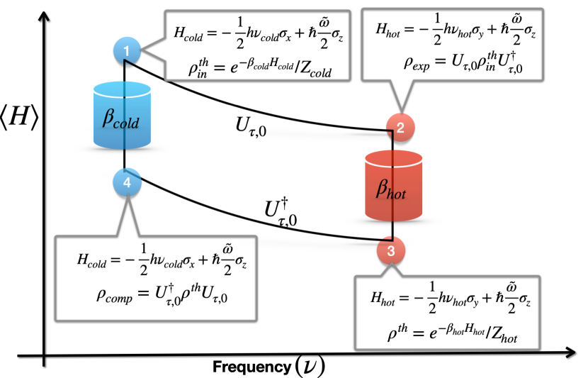
Figure 1: Schematic diagram of four-stroke Otto cycle. The path $1\rightarrow 2$ indicates the expansion stroke, $2\rightarrow 3$ heating stroke, while $3\rightarrow 4$ represents the compression stroke and $4\rightarrow 1$ is the cooling stroke. States and the corresponding Hamiltonian in each stroke are mentioned. Note that $1\rightarrow 2$ and $3\rightarrow 4$ evolve unitarily.

1. Cooling stroke. For a given Hamiltonian, $H_{cold}$, the working medium is initially prepared in a thermal state, i.e., $\rho^{th}_{in}=e^{-\beta_{cold}H_{cold}}/Z_{cold}$, where $\beta_{\text{cold}}=1/{k_{B}T_{\text{cold}}}$ with $k_{B}$ being the Boltzmann constant and $T_{\text{cold}}$ being the cold effective spin temperature, and $Z_{\text{cold}}=\Tr[e^{-\beta_{cold}H_{cold}}]$ represents the partition function. Unlike the previous works de Assis et al. (2019), the Hamiltonian corresponding to the equilibrium state can be represented as $H_{\text{cold}}=-\frac{1}{2}h\nu_{\text{cold}}\sigma_{x}+\hbar\frac{\tilde{\omega}}{2}\sigma_{z}$ where $h$ is the Planck constant, $\hbar=\frac{h}{2\pi}$ and $\nu_{\text{cold}}$ is the frequency, fixed by the physical system where the experiment can be performed, $\sigma_{i}$ $(i=x,y,z)$ represents the Pauli matrices, and $\tilde{\omega}$ is the strength of the magnetic field in the z-direction whose details is described below.

2. Expansion stroke. The system evolves from time, $t=0$ to $t=\tau$ according to the Hamiltonian,

$$H_{exp}(t)=-\frac{1}{2}h\nu(t)\Big{[}\sigma_{x}\cos wt+\sigma_{y}\sin wt\Big{]}+\hbar\sigma_{z}\frac{\tilde{\omega}}{2},$$ (1)

where $\omega=\frac{\pi}{2\tau}$, thereby ensuring a full rotation of the magnetic field from $x$- to $y$-direction Peterson et al. (2019); Denzler and Lutz (2020), $\nu(t)=\nu_{cold}\Big{[}1-\left(\frac{t}{\tau}\right)\Big{]}+\nu_{hot}\left(\frac{t}{\tau}\right)$ which reflects how the energy spacing widens from $\nu_{cold}$ at time $t=0$ to $\nu_{hot}$ at $t=\tau$, and additionally, we consider a constant magnetic field with strength $\frac{\tilde{\omega}}{2}$ and $\tilde{\omega}=\mathbf{g}\omega$ with $\mathbf{g}$ being a constant. The final evolution time, $\tau$, is fixed by the experiment performed. Moreover, $\tau$ should be chosen to be much shorter than the decoherence time, so that the evolution can be performed via unitary operator Batalhão et al. (2014, 2015). Note that the driving Hamiltonian which has only rotating magnetic field with varying strength $\nu(t)$ in the $(x,y)$-plane are used to design quantum heat engines Peterson et al. (2019); Batalhão et al. (2014, 2015); Nakazato et al. (2023); Denzler and Lutz (2020). We will demonstrate that the constant magnetic field, associated with the rotating field can give rise to a significant difference in the performance of QOE.

The unitary operator responsible for the dynamics, in this case, takes the form as $U_{\tau,0}=\mathcal{T}e^{-\frac{i}{\hbar}\int_{t=0}^{\tau}H_{exp}(t)dt}$ where $\mathcal{T}$ is the time-ordering parameter. At the end of the expansion stroke, i.e., at time $\tau$, the Hamiltonian reduces to

$$H_{hot}=-\frac{1}{2}h\nu_{hot}\sigma_{y}+\hbar\frac{\tilde{\omega}}{2}\sigma_{z},$$

since at $t=\tau$, $\nu(t=\tau)=\nu_{hot}$ while the resulting state becomes $\rho_{exp}=U_{\tau,0}\rho^{th}_{in}U^{\dagger}_{\tau,0}$. The transition probability ($\xi$) between the eigenstates of the Hamiltonians $H_{cold}$ and $H_{hot}$ is defined as

$$\xi=|\bra{\Psi^{hot}_{\pm}}U(t)\ket{\Psi^{cold}_{\mp}}|^{2}=|\bra{\Psi^{cold}_{\pm}}U^{\dagger}(t)\ket{\Psi^{hot}_{\mp}}|^{2},$$ (2)

where $\ket{\Psi^{hot}_{\pm}}$ and $\ket{\Psi^{cold}_{\mp}}$ are the eigenstates of $H_{hot}$ and $H_{cold}$ respectively. When the process obeys the adiabatic theorem and there is no transition between the instantaneous eigenstates of the Hamiltonian, $\xi$ vanishes. Due to the transition between the instantaneous eigenstates of the Hamiltonian (i.e., associated with a finite time), the irreversibility is introduced in the QOE which leads to the low performance for general quantum engine protocol when both the thermal reservoirs are at a positive spin temperature Peterson et al. (2019); Plastina et al. (2014); Cakmak et al. (2017). Interestingly, when one considers two reservoirs having a positive and an effective negative spin temperatures, the performance of the QOE is enhanced de Assis et al. (2019).

3. Heating stroke. This is again a thermalization process (see $2\rightarrow 3$ step in Fig. 1) in which the state reaches to the equilibrium state corresponding to the Hamiltonian, $H_{hot}$, represented as $\rho^{th}=e^{-\beta_{hot}H_{hot}}/\Tr[e^{-\beta_{hot}H_{hot}}]$. It occurs through the heat exchange between the working medium and the bath.

4. Compression stroke. It is the fourth stroke of the Otto cycle and is the reverse process of the expansion in which an energy gap compression is attained Camati and Serra (2018); Campisi et al. (2011); Kieu (2004). Therefore, time-reversed protocol of the expansion stroke occurs such that the Hamiltonian can be written as $H_{comp}(t)=-H_{exp}(\tau-t)$. As in the case of expansion, it can also be assumed to be unitary, denoted as $U^{\dagger}_{\tau,0}$. The compression stroke acts on $\rho^{th}$ and leads to the final state as $\rho_{comp}=U^{\dagger}_{\tau,0}\rho^{th}U_{\tau,0}$ in which the Hamiltonian can be written as

$$H_{cold}=-\frac{1}{2}h\nu_{cold}\sigma_{x}+\hbar\frac{\tilde{\omega}}{2}\sigma_{z}$$

since at $t=0$, $\nu({t=0})=\nu_{cold}$.

III Enhanced Efficiency via constant magnetic field

III.1 Transition Probability

To establish the role of additional magnetic field in the performance of QOE, let us now investigate the effects of $\mathbf{g}$ in $\tilde{\omega}$ on the transition probability and the efficiency of QOE. To obtain the transition probability, $\xi$ in Eq. (2), we use the eigenvalue equation of $H_{cold(hot)}$ corresponding to the eigenstate $\ket{\Psi^{cold(hot)}_{\pm}}$ as

$$H_{cold(hot)}\ket{\Psi^{cold(hot)}_{\pm}}$$

$$=\pm\frac{h}{4\pi}\sqrt{4\pi^{2}\nu^{2}_{cold(hot)}+\tilde{\omega}^{2}}\ket{\Psi^{cold(hot)}_{\pm}}$$

$$=\pm E_{cold(hot)}\ket{\Psi^{cold(hot)}_{\pm}}$$ (3)

where $E_{cold(hot)}=\frac{h}{4\pi}\sqrt{4\pi^{2}\nu^{2}_{cold(hot)}+\tilde{\omega}^{2}}$. Let us rewrite the Hamiltonian for the dynamics in step 2, i.e.,

$$H_{exp}(t)= -\frac{1}{2}h\nu(t)\Big{[}\sigma_{x}\cos wt+\sigma_{y}\sin wt\Big{]}+\hbar\sigma_{z}\frac{\tilde{\omega}}{2}$$

$$= -\frac{1}{2}h\nu(t)\Big{[}(\sigma_{+}+\sigma_{-})\cos wt+(\sigma_{+}-\sigma_{-})\sin wt\Big{]}$$

$$~{}~{}~{}~{}~{}~{}~{}~{}~{}~{}~{}~{}~{}~{}~{}~{}~{}~{}~{}~{}~{}~{}~{}~{}~{}~{}~{}~{}~{}~{}~{}~{}~{}~{}~{}~{}~{}~{}~{}~{}~{}~{}~{}~{}~{}~{}~{}~{}~{}~{}~{}+\hbar\sigma_{z}\frac{\tilde{\omega}}{2}$$

$$= -\frac{1}{2}h\nu(t)\Big{[}e^{-i\frac{\omega}{2}\sigma_{z}t}\sigma_{x}e^{i\frac{\omega}{2}\sigma_{z}t}\Big{]}+\hbar\sigma_{z}\frac{\tilde{\omega}}{2},$$ (4)

where $\sigma_{\pm}=\frac{1}{2}\left(\sigma_{x}\pm i\sigma_{y}\right)$. Now from the equation, $i\hbar\frac{dU(t,0)}{dt}=H_{exp}(t)U(t,0)$ for the Hamiltonian of above Eq. (III.1) we can get

$$i\frac{dU^{\prime}(t,0)}{dt}=\left[-\pi\nu(t)\sigma_{x}+\left(\frac{\tilde{\omega}}{2}-\frac{\omega}{2}\right)\sigma_{z}\right]U^{\prime}(t,0),$$ (5)

where $U^{\prime}(t,0)=e^{i\frac{\omega}{2}\sigma_{z}t}U(t,0)$. If we consider the same magnetic strength for rotating axis and z-axis, i.e, $\tilde{\omega}=\omega$, it is very straight forward. In this article, we are curious about the the case when $\tilde{\omega}\neq\omega$. The principle question that we want to investigate is whether there is any advantage of taking $\tilde{\omega}$ instead of taking $\omega$.
We can write the time-evolution operator corresponding to Hamiltonian as Barnes and Das Sarma (2012); Barnes (2013)

$$U=\begin{pmatrix}u_{11}&-u^{*}_{21}\\ u_{21}&u^{*}_{11}\end{pmatrix},~{}~{}~{}|u_{11}|^{2}+|u_{21}|^{2}=1,$$ (6)

and we transform the unitary to a rotating x-basis. We have

$$D_{\pm}=\frac{1}{\sqrt{2}}e^{\pm iJ(t)}\{u_{11}(t)\pm u_{21}(t)\}$$ (7)

where $J(t)=\int_{0}^{t}-\pi\nu(t^{\prime})dt^{\prime}$. By solving the Schr$\ddot{o}$dinger equation, we get

$$\dot{D}_{\pm}(t)=-i\left(\frac{\tilde{\omega}}{2}-\frac{\omega}{2}\right)e^{\pm 2iJ(t)}D_{\mp}(t).$$ (8)

For the Hamiltonian where $\tilde{\omega}=\omega$, and from this first order differential equation, we can construct the unitary which alike with the unitary of Ref. Denzler and Lutz (2020). For our case, we go to the second order differential equation for $D_{+}$ which is

$$\ddot{D}_{+}(t)+2i\pi\nu(t)\dot{D}_{+}(t)+\left(\frac{\tilde{\omega}}{2}-\frac{\omega}{2}\right)^{2}D_{+}(t)=0.$$ (9)

By solving the above differential equation, we can obtain the unitary operator, $U_{\tau,0}$ which leads to the transition probability $\xi$ between the energy eigenstate of $H_{cold}$ and $H_{exp}$ during the compression stroke. The transition probability, $\xi$, with driving time, $\tau$ is shown in Fig. 2.

Unlike the conventional Hamiltonian considered in QOE (without constant magnetic field in the $z$-direction), $\xi$ increases with the expansion (compression) time, $\tau$ and then decreases with $\tau$ as is the case for Hamiltonian with $\tilde{\omega}=0$. For a certain nonvanishing $\mathbf{g}$ values, we clearly find that there exists a range of driving time, $\tau$, such that $\xi(\mathbf{g}>0)>\xi(\mathbf{g}=0)$ (see Fig. 2). It is also noted that such advantage decreases with the increase of $\mathbf{g}$ and high value of $\tau$. Notice that the net work of the cycle, and hence the efficiency of QOE is related to $\xi$. Therefore, we can expect that if we choose $\tau$ close to the case with $\xi$ being maximum or higher than the one obtained with $\mathbf{g}=0$, the efficiency can be enhanced. We will now manifest that this is indeed the case. For demonstration, we choose those set of parameters which are used in NMR experiment de Assis et al. (2019); Peterson et al. (2019) so that the benefit of additional magnetic field can be illustrated.

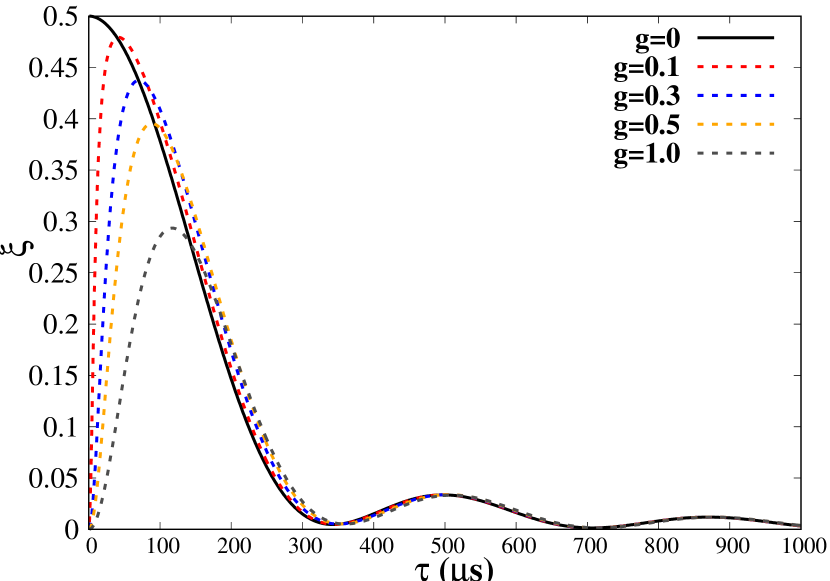
Figure 2: Transition probability ($\xi$) (ordiante) with respect to driving time $\tau$ (abscissa) for different strengths of the magnetic field in the $z$ direction ($\mathbf{g}$). The driving time is taken in microseconds and the ordinate is dimensionless. We take $\nu_{cold}=2.0$ and $\nu_{hot}=3.6kHz$. For $\mathbf{g}=0$, $\xi$ is plotted in solid line and for higher $\mathbf{g}$ values, it is plotted in dashed lines.

III.2 Calculate the Efficiency

Before computing the net work and efficiency, let us define the local temperature in terms of population as

$$\beta_{cold(hot)}=\frac{1}{h\sqrt{\nu^{2}_{cold(hot)}+(\frac{\tilde{\omega}}{2\pi}})^{2}}\ln\left(\frac{1-p^{+}_{cold(hot)}}{p^{+}_{cold(hot)}}\right)$$ (10)

where $p^{+}_{cold(hot)}=\bra{\Psi^{cold(hot)}_{+}}\rho^{th}_{in}(\rho^{th})\ket{\Psi^{cold(hot)}_{+}}$. When the population of high energy states exceeds the population of low-energy states, the effective temperature becomes negative. From Eq. (10), we get that $p^{+}_{cold(hot)}\in[0,0.5)$ leads to $\beta_{cold(hot)}$ to be positive while $p^{+}_{cold(hot)}\in[0.5,1.0)$, thereby giving $\beta_{cold(hot)}$ negative. It was already shown that QOE can be efficient, when $\beta_{cold(hot)}$ takes negative values de Assis et al. (2019). In our analysis, we vary $p^{+}_{hot}$ within $0.5$ and $1.0$ by fixing $p^{+}_{cold}=0.261$.

Let us first compute the partition function,

$$Z_{cold(hot)}= \Tr[e^{-\beta_{cold(hot)}H_{cold(hot)}}]$$

$$= 2\cosh\left(\beta_{cold(hot)}E_{cold(hot)}\right).$$

Now to derive the QOE efficiency($\eta$), we have to calculate the average net work $\langle W\rangle$ performed by the QOE and then the average heat $\langle Q_{hot}\rangle$. Lets calculate them with the constraints $\beta_{cold}>0$ and $\beta_{hot}<0~{}(\beta_{hot}=-|\beta_{hot}|)$. The detail calculations are done in Appendix (A). The net work of the cycle occurs during $1\rightarrow 2$ and $3\rightarrow 4$. Hence it is defined as

$$\langle W\rangle= \langle W_{1\rightarrow 2}\rangle+\langle W_{3\rightarrow 4}\rangle$$

$$= \Tr[\rho_{exp}H_{hot}]-\Tr[\rho^{th}_{in}H_{cold}]+\Tr[\rho_{comp}H_{cold}]$$

$$-\Tr[\rho^{th}H_{hot}]$$

$$= \Xi_{1}+\xi~{}\Xi_{2}$$ (12)

where

$$\Xi_{1}=(E_{cold}-E_{hot})\left[\tanh(\beta_{cold}E_{cold})+\tanh(|\beta_{hot}|E_{hot})\right]$$

and

$$\Xi_{2}=2\left[E_{hot}\tanh(\beta_{cold}E_{cold})-E_{cold}\tanh(|\beta_{hot}|E_{hot})\right]$$

while the heat exchanged between the working medium and the hot as well cold reservoirs happens during other steps since they cannot take place simultaneously, i.e., during $3\rightarrow 2$ and $4\rightarrow 1$. They are respectively given by

$$\langle Q_{hot}\rangle= \langle Q_{3\rightarrow 2}\rangle$$

$$= \Tr[\rho^{th}H_{hot}]-\Tr[\rho_{exp}H_{hot}]$$

$$= \Pi_{1}-\xi~{}\Pi_{2}$$ (13)

where

$$\Pi_{1}=E_{hot}\left[\tanh(\beta_{cold}E_{cold})+\tanh(|\beta_{hot}|E_{hot})\right]$$

and

$$\Pi_{2}=2\left[E_{hot}\tanh(\beta_{cold}E_{cold})\right]$$

In addition,

$$\langle Q_{cold}\rangle= \langle Q_{4\rightarrow 1}\rangle$$

$$= \Tr[\rho^{th}_{in}H_{cold}]-\Tr[\rho_{comp}H_{cold}]$$

$$= \Pi_{3}+\xi~{}\Pi_{4}$$ (14)

where

$$\Pi_{3}=-E_{cold}\left[\tanh(\beta_{cold}E_{cold})+\tanh(|\beta_{hot}|E_{hot})\right]$$

and

$$\Pi_{4}=2\left[E_{cold}\tanh(|\beta_{hot}|E_{hot})\right].$$

Before we calculate the efficiency, we can note that the net work depends on transition probability in Eq. (III.2). Therefore, we can expect a better efficiency if we choose $\xi$ for a proper $\mathbf{g}$ value (see Fig. 2) as such which is more than the $\mathbf{g}=0$. The efficiency in terms of net work and heat can be computed analytically (see Appendix A) as

$$\eta= -\frac{\langle W\rangle}{\langle Q_{hot}\rangle}$$

$$= 1-\frac{E_{cold}}{E_{hot}}\left(\frac{1-2\xi\mathcal{F}}{1-2\xi\mathcal{G}}\right)$$

Here

$$\hskip 36.135pt\mathcal{F}=\frac{\tanh\left(|\beta_{hot}|E_{hot}\right)}{\tanh\left(\beta_{cold}E_{cold}\right)+\tanh\left(|\beta_{hot}|E_{hot}\right)},$$ (16)

and

$$\mathcal{G}=\frac{\tanh\left(\beta_{cold}E_{cold}\right)}{\tanh\left(\beta_{cold}E_{cold}\right)+\tanh\left(|\beta_{hot}|E_{hot}\right)}.$$ (17)

As seen in Fig. 2, we realize that when the driving time is moderate, $\xi$ gives higher value with $\mathbf{g}>0$ than that of the system having $\mathbf{g}=0$.

Let us concentrate on $\tau\in[100,200]\,\text{in}\,\mu s$. Note that the range of $\tau$ is also chosen for demonstration in the NMR experiment of QOE de Assis et al. (2019) which implies that such driving time is accessible in the laboratory. In this regime, we observe that when $p^{+}_{hot}$ is in the neighbourhood of unity, the efficiency of QOE with system having $\mathbf{g}>0$ is higher than that of the system without the magnetic field. The small driving time leads to a higher range of $p^{+}_{hot}$ values for which $\eta(\mathbf{g}>0)>\eta(\mathbf{g}=0)$ (as depicted in Fig. 3).

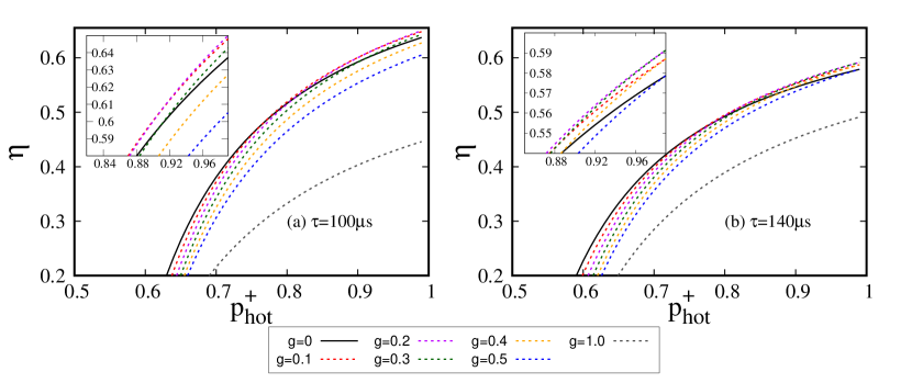
Figure 3: Efficiency, $\eta$, (ordinate) versus the population of the excited state, $p^{+}_{hot}$ (abscissa) for a fixed driving time $\tau$. Solid lines represent $\mathbf{g}=0$ and all dotted lines are for $\mathbf{g}>0$. We take $p^{+}_{cold}=0.261$ and vary $p^{+}_{hot}$ within $[0.5,1.0)$. All the other parameters are same as in Fig. 2. (left) Driving time is fixed to $\tau=100\mu s$ and (right) it is $\tau=140\mu s$. The maximum efficiency is achieved at $\mathbf{g}=0.2$ for $\tau=100\mu s$ while it is $\mathbf{g}=0.3$ when $\tau=140\mu s$. All the axes are dimensionless.

Interestingly, introduction of magnetic field is not ubiquitous to obtain a high efficiency in QOE. Specifically, there exists a critical strength of the magnetic field, $\mathbf{g}_{c}$, above which the efficiency goes below the one obtained with $\mathbf{g}=0$, when all the parameters are fixed to a certain value. For a fixed $\tau$, and $p^{+}_{cold}$, there exists a lower bound of $p^{+}_{hot}$ above which high $\eta(\mathbf{g}>0)$ is obtained. More precisely, we notice that

$$\eta(\tau=100\mu s,\mathbf{g}=0.2)-\eta(\tau=100\mu s,\mathbf{g}=0)=0.012,$$

where we fix $p^{+}_{cold}=0.261$ and $p^{+}_{hot}=0.99$ while

$$\eta(\tau=200\mu s,\mathbf{g}=0.3)-\eta(\tau=100\mu s,\mathbf{g}=0)=0.007$$

for the same set of values of $p^{+}_{cold}$ and $p^{+}_{hot}$. For $\tau=140\mu s$, the efficiency advantage we get is $0.012$ for $g=0.3$ and the other parameters $p^{+}_{cold(hot)}$ are same as above. When $\xi=0$, it represents the conventional heat engine with efficiency $\eta=1-(E_{cold}/E_{hot})$. When the expansion and compression strokes follow ideal adiabatic process, i.e., $\xi=0$, $\eta$ tends to $\eta_{Otto}$. The condition for which we can get $\eta\geq\eta_{Otto}$ is given by (see Appendix A)

$$|\beta_{hot}|\sqrt{4\pi^{2}\nu^{2}_{hot}+\tilde{\omega}^{2}}\geq\beta_{cold}\sqrt{4\pi^{2}\nu^{2}_{cold}+\tilde{\omega}^{2}}$$ (18)

Remark. Let us take $\mathbf{g}<0$ and ask whether such a benefit reported above with $\mathbf{g}>0$ persists. The answer is affirmative. We observe that with $\mathbf{g}<0$, $\eta(\mathbf{g}<0)>\eta(\mathbf{g}=0)$ upto certain values of $\mathbf{g}$. However, unlike $\mathbf{g}>0$, where the advantage is obtained when $p^{+}_{hot}\approx 1$, we find that the enhancement of $\eta$ is found, when $p^{+}_{hot}$ is close to $0.5$ with the same values of $p^{+}_{cold}$.

We will now try to find out the reason behind the advantage obtained with the addition of magnetic field in each stroke.

III.3 Coherence: An indicator of enhanced performance in QOE

Let us investigate the behavior of coherence for the expansion and compression stroke in the Otto cycle. It was indicated that the performance of four-stroke Otto cycle can be linked to coherence Feldmann and Kosloff (2006); Rezek and Kosloff (2006); Feldmann and Kosloff (2012); Thomas and Johal (2014); Correa et al. (2015); Santos et al. (2019); Francica et al. (2019). The Hamiltonian $H_{exp}(t)$ and $H_{comp}(t)$ do not commute with itself at different times, so these non-commuting Hamiltonian generates coherence in the expansion and compression strokes of the QOE while it vanishes during thermalization. Here we assume that coherence is computed in the energy eigenbasis of $H_{cold}$ and $H_{hot}$.

We quantify the coherence by $l_{1}$-norm measure which is defined as the sum of the absolute values of the off diagonal elements of a given state which is written in the eigenbasis of $H_{cold}$ and $H_{hot}$, i.e., $C_{l_{1}}(\rho)=\sum_{i\neq j}|\rho_{ij}|$ Streltsov et al. (2017). One of our goal is to examine how the coherence is affected by introducing $\tilde{\omega}$ in the driving Hamiltonian. To study this, we calculate coherence with respect to $\tau$ for different $\mathbf{g}$ values.

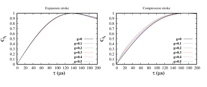
Figure 4: $l_{1}$-norm of coherence ($C_{l_{1}}$) (vertical axis) with driving time $\tau$ (horizontal axis) for different $\mathbf{g}$ values. The unit of the horizontal axis is $\mu s$ and the vertical axis is dimensionless. We calculate the coherence for $p^{+}_{hot}=0.9$. All the other specifications are same as in Fig. 3.

Specifically, during the expansion and the compression strokes, we study the trends of coherence measure with the variation of the driving time ($\tau$) for different strengths in the $z$-directional magnetic field, $\mathbf{g}$. We can observe that there exits a range of $\mathbf{g}$ for which the coherence is more than that obtained $\mathbf{g}=0$ (see Fig. 4). Since the states are different for the expansion and compression strokes, the coherence is not equal. In summary, we notice that when $\tau\in[100,200]$, the coherence generated with positive $\mathbf{g}$ is higher than the one produced without the magnetic field in the $z$-direction. However, we cannot find a close relation between $C_{l_{1}}$ and the efficiency of QOE, $\eta$.

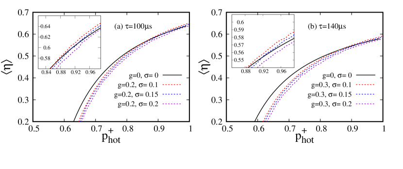
Figure 5: Quenched average efficiency, denoted as $\langle\eta\rangle$ (ordinate) against the population of the excited state, $p^{+}_{hot}$ (abscissa) for two different values of $\mathbf{g}$. $\delta_{i}$ ($i=1,2$) involved in $(1+\delta_{1})\nu_{cold}$ and $(1+\delta_{2})\nu_{hot}$ of the QOE are chosen randomly from two Gaussian distributions with zero mean and the same standard deviation, $\sigma$ for a fixed driving time $\tau$. (left) We compare $\mathbf{g}=0.2$ by varying the strength of the disorder, $\sigma$ with the QOE having $\mathbf{g}=0$ without disorder. (right) The same comparison is performed with $\mathbf{g}=0.3$. Choices of $\mathbf{g}$ is due to the observations in Fig. 3. We take all the others parameters are same as in Fig. 3. All the axes are dimensionless.

IV Robustness of Otto engine against impurities

During implementation of any quantum devices, some imperfection or impurities or noise is inevitable, thereby creating hindrances in the performance Lewenstein et al. (2007); Ahufinger et al. (2005); Konar et al. (2022); Ghoshal et al. (2020); Ghosh et al. (2020); Sanchez-Palencia and Lewenstein (2010); Breuer and Petruccione (2002); Rivas and Huelga (2012). To study such scenario, decoherence or disorder can be introduced during several steps of the engines. For example, noise can effect during the preparation of the initial state Farina et al. (2019); Ghosh et al. (2021), or imperfect unitary operator Halder et al. (2022) can also reduce the performance of the engine. Generally, disorders are often present in the engine’s control and in the measurement process Kosloff and Levy (2014). Due to impurities in the Hamiltonian, the quantum coherence may be disturbed, thereby leading to a change in efficiency. To attenuate the effects of disorder on the quantum engine, there are some approaches that can be taken like quantum error correction Knill (2005); Terhal (2015); Georgescu (2020), dynamical decoupling Viola et al. (1999); Álvarez and Suter (2011b), and robust control methods Daoyi Dong (2023); Shermer (2023). Further, the current experimental developments also give rise to the possibility to probe properties of such disordered models where disorder can be added in the system.

Let us check the effect of disorder on the design of four-stroke engine presented in the preceding section. To introduce disorder in the model, a single or several parameters involved in the model are chosen randomly, and one then preforms averaging of the quantity of interest which, in this case, is efficiency in over large number of configurations - quenched averaging. In this scenario, it is assumed that the observation time of some parameters is much smaller than the time taken by the same set of parameters to reach the equilibrium. Quenched disorder typically creates a energy landscape with many local minima and it confines the system in a metastable state, thereby remaining in one of the local minima for a long time Sethna (2006); Bouchaud (1992); Fisher and Huse (1988); Binder and Young (1986); Suzuki et al. (2013); Sachdev (2011); B.K.Chakrabarti et al. (1996); M. Mezard and Virasoro (1987); Chowdhury (1986).

We here incorporate disorder in the frequency of the ideal system, $\nu_{cold}$ and $\nu_{hot}$ as $(1+\delta_{1})\nu_{cold}$ and $(1+\delta_{2})\nu_{hot}$. Here $\delta_{1(2)}$ is chosen from two different Gaussian distributions having same vanishing mean and standard deviation $\sigma$ which can be called strength of the disorder. The probability density function for Gaussian disorder with vanishing mean and standard deviation, $\sigma$ is given by $P(\delta_{i})=\frac{1}{\sigma\sqrt{2\pi}}e^{-\frac{1}{2}(\frac{\delta_{i}}{\sigma})^{2}},~{}~{}-\infty\leq\delta\leq\infty$. The quenched averaged efficiency for a given strength of disorder, $\sigma$ can be written as

$$\langle\eta(\sigma)\rangle=\int P(\delta_{1})P(\delta_{2})\eta\left(\nu_{cold}(1+\delta_{1}),\nu_{hot}(1+\delta_{2})\right)d\delta_{1}\delta_{2}.$$

We have already shown that in presence of magnetic field in the z-direction, the efficiency of the four-stroke machine can be improved. We now want to find out whether even in presence of disorder, the advantage persists or not. For comparison, we take the system with $\mathbf{g}=0$ without disorder. For a fixed driving time, a fixed $\mathbf{g}>0$ and $p^{+}_{cold}$, we compute the quenched average efficiency, $\langle\eta\rangle$ by varying $p^{+}_{hot}$ for different values of disorder strength. We observe that the efficiency slightly decreases in presence of impurities in $\nu_{hot}$ and $\nu_{cold}$. However, we find that if the strength of the disorder is moderate, $\langle\eta\rangle$ is higher than that can be obtained by the system with $\mathbf{g}=0$ (as shown in Fig. 5).

Again, there is a trade-off relation between $\sigma$ and the driving time $\tau$. Surprisingly, the robustness of this QOE based on effective negative temperature increases with the increase of $p^{+}_{hot}$ (in Fig. 5, compare $\langle\eta\rangle$ when $p^{+}_{hot}\sim 0.5$ and $p^{+}_{hot}\sim 1.0$ ). We emphasis here that the four-stroke quantum Otto engine can be shown to be robust against disorder, when parameters are chosen both from Gaussian and uniform distributions, given by ($P(\delta)=\frac{1}{\sigma},~{}~{}\text{when}-\frac{\sigma}{2}\leq\delta\leq\frac{\sigma}{2}$ and $=0,\,\text{otherwise}$ (for illustration, we only consider Gaussian disorder in Fig. 5).

V Conclusion

The performance of the thermal machines like heat engines, refrigerators, and batteries can be shown to be enhanced if one builds these devices by using quantum mechanical systems. A four-stroke quantum Otto engine is the main focus of this work. In this respect, it was shown recently that the efficiency of the engines working under thermal reservoirs having effective negative and positive temperatures can be improved in comparison to the engines having reservoirs with positive temperatures.

Summarising, we build a quantum Otto engine in which the four strokes involve additional magnetic fields in the $z$-direction and the rotating magnetic field applied in the $(x,y)$-plane. We explored that by manipulating the strength of the additional magnetic field and other parameters involved in the system, we can enhance efficiency compared to the one without the magnetic field in the $z$-direction. We analytically compute the transition probability, total work, and the average heat which leads to a closed form expression of the efficiency in the engine. We found that the increase in strength of the additional magnetic field does not universally increase the efficiency. A critical strength of the constant magnetic field exists for a fixed driving time. With a very high driving time, such an advantage disappears. We argued that generated coherence in the expansion and compression strokes and the transition probability for a moderate driving time can be accountable for the gain in efficiency of the proposed quantum Otto engine.

Realization of any quantum devices suffers imperfections or impurities during building or during the running of the engines. We showed that the frequency involved in all the strokes has some disorder. We observed that if such parameters are chosen randomly from Gaussian or uniform distribution, the quenched averaged efficiency can still be higher than the system without a constant magnetic field. It illustrates that the quantum Otto engine presented here is robust against impurities. The results obtained here indicate that the performance of the quantum heat engines can be improved even by locally tunable properties like the coherence of the system.

VI Acknowledgment

We acknowledge the support from the Interdisciplinary Cyber-Physical Systems (ICPS) program of the Department of Science and Technology (DST), India, Grant No.: DST/ICPS/QuST/Theme- 1/2019/23.

Appendix A Computation of efficiency via net work and heat

The net work of the cycle in the four-stroke QOE can be defined as

$$\langle W\rangle= \langle W_{1\rightarrow 2}\rangle+\langle W_{3\rightarrow 4}\rangle$$

$$= \Tr[\rho_{exp}H_{hot}]-\Tr[\rho^{th}_{in}H_{cold}]+\Tr[\rho_{comp}H_{cold}]$$

$$-\Tr[\rho^{th}H_{hot}].$$

On the other hand, the heats exchanged between the working medium and the hot reservoir can be written as

$$\langle Q_{hot}\rangle= \langle Q_{3\rightarrow 2}\rangle$$

$$= \Tr[\rho^{th}H_{hot}]-\Tr[\rho_{exp}H_{hot}].$$ (19)

When the heat exchange occurs between the medium and cold reservoir, the above quantity takes the form as

$$\langle Q_{cold}\rangle= \langle Q_{4\rightarrow 1}\rangle$$

$$= \Tr[\rho^{th}_{in}H_{cold}]-\Tr[\rho_{comp}H_{cold}].$$ (20)

Let us analytically compute the each quantity involved in the definition of heat and net work.

$$\Tr[\rho_{exp}H_{hot}]= \Big{[}-\frac{h}{4\pi}\sqrt{4\pi^{2}\nu^{2}_{hot}+\tilde{\omega}^{2}}~{}~{}\tanh\left(\beta_{cold}\frac{h}{4\pi}\sqrt{4\pi^{2}\nu^{2}_{cold}+\tilde{\omega}^{2}}\right)\left(1-2\xi\right)\Big{]},$$

$$= -E_{hot}\tanh(\beta_{cold}E_{cold})\left(1-2\xi\right),$$ (21)

$$\Tr[\rho_{comp}H_{cold}]= \Big{[}-\frac{h}{4\pi}\sqrt{4\pi^{2}\nu^{2}_{cold}+\tilde{\omega}^{2}}~{}~{}\tanh\left(\beta_{hot}\frac{h}{4\pi}\sqrt{4\pi^{2}\nu^{2}_{hot}+\tilde{\omega}^{2}}\right)\left(1-2\xi\right)\Big{]},$$

$$= -E_{cold}\tanh(\beta_{hot}E_{hot})\left(1-2\xi\right),$$ (22)

and

$$\Tr[\rho^{th}_{in}H_{cold}]= \Big{[}-\frac{h}{4\pi}\sqrt{4\pi^{2}\nu^{2}_{cold}+\tilde{\omega}^{2}}~{}~{}\tanh\left(\beta_{cold}\frac{h}{4\pi}\sqrt{4\pi^{2}\nu^{2}_{cold}+\tilde{\omega}^{2}}\right)\Big{]},$$

$$= -E_{cold}\tanh(\beta_{cold}E_{cold}),$$ (23)

and

$$\Tr[\rho^{th}H_{hot}]= \Big{[}-\frac{h}{4\pi}\sqrt{4\pi^{2}\nu^{2}_{hot}+\tilde{\omega}^{2}}~{}~{}\tanh\left(\beta_{hot}\frac{h}{4\pi}\sqrt{4\pi^{2}\nu^{2}_{hot}+\tilde{\omega}^{2}}\right)\Big{]},$$

$$= -E_{hot}\tanh(\beta_{hot}E_{hot}).$$ (24)

With the help of the above quantities, we can arrive at the expression of the $\langle W\rangle$, $\langle Q_{hot}\rangle$ and $\langle Q_{cold}\rangle$ as

$$\langle W\rangle=\left(E_{cold}-E_{hot}\right) \Big{[}\tanh(\beta_{cold}E_{cold})-\tanh(\beta_{hot}E_{hot})\Big{]}+$$ (25)

$$2\xi\Big{[}E_{hot}\tanh(\beta_{cold}E_{cold})+E_{cold}\tanh(\beta_{hot}E_{hot})\Big{]},$$

$$\langle Q_{hot}\rangle=E_{hot}\Big{[}\tanh(\beta_{cold}E_{cold})-\tanh(\beta_{hot}E_{hot})\Big{]}-2\xi\Big{[}E_{hot}\tanh(\beta_{cold}E_{cold})\Big{]},$$ (26)

and

$$\langle Q_{cold}\rangle=-E_{cold}\Big{[}\tanh(\beta_{cold}E_{cold})-\tanh(\beta_{hot}E_{hot})\Big{]}-2\xi\Big{[}E_{cold}\tanh(\beta_{hot}E_{hot})\Big{]}.$$ (27)

Now by considering $\beta_{cold}>0$ and $\beta_{hot}<0~{}(\beta_{hot}=-|\beta_{hot}|)$, the above expressions reduces to

$$\langle W\rangle=\left(E_{cold}-E_{hot}\right) \Big{[}\tanh(\beta_{cold}E_{cold})+\tanh(|\beta_{hot}|E_{hot})\Big{]}+$$ (28)

$$2\xi\Big{[}E_{hot}\tanh(\beta_{cold}E_{cold})-E_{cold}\tanh(|\beta_{hot}|E_{hot})\Big{]},$$

$$\langle Q_{hot}\rangle=E_{hot}\Big{[}\tanh(\beta_{cold}E_{cold})+\tanh(|\beta_{hot}|E_{hot})\Big{]}-2\xi\Big{[}E_{hot}\tanh(\beta_{cold}E_{cold})\Big{]},$$ (29)

and

$$\langle Q_{cold}\rangle=-E_{cold}\Big{[}\tanh(\beta_{cold}E_{cold})+\tanh(|\beta_{hot}|E_{hot})\Big{]}+2\xi\Big{[}E_{cold}\tanh(|\beta_{hot}|E_{hot})\Big{]}.$$ (30)

With the help of the above quantities, we can arrive at the expression of the efficiency as

$$\eta= -\frac{\langle W\rangle}{\langle Q_{hot}\rangle}$$

$$= \frac{\left(E_{cold}-E_{hot}\right)\Big{[}\tanh(\beta_{cold}E_{cold})+\tanh(|\beta_{hot}|E_{hot})\Big{]}+2\xi\Big{[}E_{hot}\tanh(\beta_{cold}E_{cold})-E_{cold}\tanh(|\beta_{hot}|E_{hot})\Big{]}}{E_{hot}\Big{[}\tanh(\beta_{cold}E_{cold})+\tanh(|\beta_{hot}|E_{hot})\Big{]}-2\xi\Big{[}E_{hot}\tanh(\beta_{cold}E_{cold})\Big{]}}$$

$$= 1-\frac{E_{cold}}{E_{hot}}\left(\frac{1-2\xi\mathcal{F}}{1-2\xi\mathcal{G}}\right).$$ (31)

Here, let us define $F$ and $G$ as

$$\mathcal{F}= \frac{\tanh\left(|\beta_{hot}|E_{hot}\right)}{\tanh\left(\beta_{cold}E_{cold}\right)+\tanh\left(|\beta_{hot}|E_{hot}\right)},$$ (32)

and

$$\mathcal{G}= \frac{\tanh\left(\beta_{cold}E_{cold}\right)}{\tanh\left(\beta_{cold}E_{cold}\right)+\tanh\left(|\beta_{hot}|E_{hot}\right)}.$$ (33)

Let us now find out the condition for which we can get $\eta\geq\eta_{Otto}$ in the form of $F$ and $G$, i.e. ,

$$1-\frac{E_{cold}}{E_{hot}}\left(\frac{1-2\xi\mathcal{F}}{1-2\xi\mathcal{G}}\right) \geq 1-\frac{E_{cold}}{E_{hot}}$$

$$\implies\left(\frac{1-2\xi\mathcal{F}}{1-2\xi\mathcal{G}}\right) \leq 1$$

$$\implies F \geq G$$

$$\implies\tanh\left(|\beta_{hot}|\frac{h}{4\pi}\sqrt{4\pi^{2}\nu^{2}_{hot}+\tilde{\omega}^{2}}~{}\right) \geq \tanh\left(\beta_{cold}\frac{h}{4\pi}\sqrt{4\pi^{2}\nu^{2}_{cold}+\tilde{\omega}^{2}}~{}\right)$$

$$\implies|\beta_{hot}|\sqrt{4\pi^{2}\nu^{2}_{hot}+\tilde{\omega}^{2}} \geq \beta_{cold}\sqrt{4\pi^{2}\nu^{2}_{cold}+\tilde{\omega}^{2}}.$$ (34)

References

- Peña et al. (2020) F. J. Peña, O. Negrete, N. Cortés, and P. Vargas, Entropy 22 (2020), 10.3390/e22070755.
- Scovil and Schulz-DuBois (1959) H. E. D. Scovil and E. O. Schulz-DuBois, Phys. Rev. Lett. 2, 262 (1959).
- Jochen Gemmer (2009) G. M. Jochen Gemmer, M. Michel, Quantum Thermodynamics (Springer Berlin, Heidelberg, 2009).
- Deffner and Campbell (2019) S. Deffner and S. Campbell, Quantum Thermodynamics, 2053-2571 (Morgan & Claypool Publishers, 2019).
- Myers et al. (2022) N. M. Myers, O. Abah, and S. Deffner, AVS Quantum Science 4, 027101 (2022), https://doi.org/10.1116/5.0083192 .
- Scully et al. (2003) M. O. Scully, M. S. Zubairy, G. S. Agarwal, and H. Walther, Science 299, 862 (2003).
- Klaers et al. (2017) J. Klaers, S. Faelt, A. Imamoglu, and E. Togan, Phys. Rev. X 7, 031044 (2017).
- de Assis et al. (2021) R. J. de Assis, J. S. Sales, U. C. Mendes, and N. G. de Almeida, Journal of Physics B: Atomic, Molecular and Optical Physics 54, 095501 (2021).
- Zhang (2020) Y. Zhang, Physica A: Statistical Mechanics and its Applications 559, 125083 (2020).
- Tabatabaei et al. (2022) S. M. Tabatabaei, D. Sánchez, A. L. Yeyati, and R. Sánchez, Phys. Rev. B 106, 115419 (2022).
- Hardal et al. (2017) A. U. C. Hardal, N. Aslan, C. M. Wilson, and O. E. Müstecaplıoğlu, Phys. Rev. E 96, 062120 (2017).
- Scully (2001) M. O. Scully, Phys. Rev. Lett. 87, 220601 (2001).
- Huang et al. (2012) X. L. Huang, T. Wang, and X. X. Yi, Phys. Rev. E 86, 051105 (2012).
- Zagoskin et al. (2012) A. M. Zagoskin, S. Savel’ev, F. Nori, and F. V. Kusmartsev, Phys. Rev. B 86, 014501 (2012).
- Roßnagel et al. (2014) J. Roßnagel, O. Abah, F. Schmidt-Kaler, K. Singer, and E. Lutz, Phys. Rev. Lett. 112, 030602 (2014).
- Altintas et al. (2014) F. Altintas, A. U. C. Hardal, and O. E. Müstecaplıog~lu, Phys. Rev. E 90, 032102 (2014).
- Long and Liu (2015) R. Long and W. Liu, Phys. Rev. E 91, 062137 (2015).
- Xiao and Li (2018) B. Xiao and R. Li, Physics Letters A 382, 3051 (2018).
- Niedenzu et al. (2018) W. Niedenzu, V. Mukherjee, A. Ghosh, A. G. Kofman, and G. Kurizki, Nature Communications 9, 165 (2018).
- Wang et al. (2019) J. Wang, J. He, and Y. Ma, Phys. Rev. E 100, 052126 (2019).
- de Assis et al. (2020) R. J. de Assis, J. S. Sales, J. A. R. da Cunha, and N. G. de Almeida, Phys. Rev. E 102, 052131 (2020).
- Wright et al. (2018) J. S. S. T. Wright, T. Gould, A. R. R. Carvalho, S. Bedkihal, and J. A. Vaccaro, Phys. Rev. A 97, 052104 (2018).
- Murch et al. (2013) K. W. Murch, S. J. Weber, K. M. Beck, E. Ginossar, and I. Siddiqi, Nature 499, 62 (2013).
- Carvalho et al. (2001) A. R. R. Carvalho, P. Milman, R. L. de Matos Filho, and L. Davidovich, Phys. Rev. Lett. 86, 4988 (2001).
- Werlang et al. (2008) T. Werlang, R. Guzmán, F. O. Prado, and C. J. Villas-Bôas, Phys. Rev. A 78, 033820 (2008).
- Pielawa et al. (2007) S. Pielawa, G. Morigi, D. Vitali, and L. Davidovich, Phys. Rev. Lett. 98, 240401 (2007).
- Werlang and Villas-Boas (2008) T. Werlang and C. J. Villas-Boas, Phys. Rev. A 77, 065801 (2008).
- Prado et al. (2009) F. O. Prado, E. I. Duzzioni, M. H. Y. Moussa, N. G. de Almeida, and C. J. Villas-Bôas, Phys. Rev. Lett. 102, 073008 (2009).
- Verstraete et al. (2009) F. Verstraete, M. M. Wolf, and J. Ignacio Cirac, Nature Physics 5, 633 (2009).
- Hama et al. (2018) Y. Hama, W. J. Munro, and K. Nemoto, Phys. Rev. Lett. 120, 060403 (2018).
- Lovrić et al. (2007) M. Lovrić, H. G. Krojanski, and D. Suter, Phys. Rev. A 75, 042305 (2007).
- Álvarez and Suter (2011a) G. A. Álvarez and D. Suter, Phys. Rev. Lett. 107, 230501 (2011a).
- Mendonça et al. (2020) T. M. Mendonça, A. M. Souza, R. J. de Assis, N. G. de Almeida, R. S. Sarthour, I. S. Oliveira, and C. J. Villas-Boas, Phys. Rev. Res. 2, 043419 (2020).
- Ollivier and Zurek (2001) H. Ollivier and W. H. Zurek, Phys. Rev. Lett. 88, 017901 (2001).
- Oppenheim et al. (2002) J. Oppenheim, M. Horodecki, P. Horodecki, and R. Horodecki, Phys. Rev. Lett. 89, 180402 (2002).
- Horodecki et al. (2005) M. Horodecki, P. Horodecki, R. Horodecki, J. Oppenheim, A. Sen(De), U. Sen, and B. Synak-Radtke, Phys. Rev. A 71, 062307 (2005).
- Bera et al. (2017) A. Bera, T. Das, D. Sadhukhan, S. S. Roy, A. Sen(De), and U. Sen, Reports on Progress in Physics 81, 024001 (2017).
- Dillenschneider and Lutz (2009) R. Dillenschneider and E. Lutz, Europhysics Letters 88, 50003 (2009).
- Perarnau-Llobet et al. (2015) M. Perarnau-Llobet, K. V. Hovhannisyan, M. Huber, P. Skrzypczyk, N. Brunner, and A. Acín, Phys. Rev. X 5, 041011 (2015).
- Breeze (2019) P. Breeze, in Power Generation Technologies (Third Edition), edited by P. Breeze (Newnes, 2019) third edition ed., pp. 99–119.
- Heywood (2018) J. B. Heywood, Internal Combustion Engine Fundamentals (McGraw-Hill Education, 2018).
- Hill and Peterson (1991) P. Hill and C. Peterson, Mechanics and Thermodynamics of Propulsion (PEARSON, 1991).
- Stone (1985) R. Stone, Introduction to Internal Combustion Engines (M. MACMILLAN, 1985).
- de Assis et al. (2019) R. J. de Assis, T. M. de Mendonça, C. J. Villas-Boas, A. M. de Souza, R. S. Sarthour, I. S. Oliveira, and N. G. de Almeida, Phys. Rev. Lett. 122, 240602 (2019).
- Nettersheim et al. (2022) J. Nettersheim, S. Burgardt, Q. Bouton, D. Adam, E. Lutz, and A. Widera, PRX Quantum 3, 040334 (2022).
- Peterson et al. (2019) J. P. S. Peterson, T. B. Batalhão, M. Herrera, A. M. Souza, R. S. Sarthour, I. S. Oliveira, and R. M. Serra, Phys. Rev. Lett. 123, 240601 (2019).
- Streltsov et al. (2017) A. Streltsov, G. Adesso, and M. B. Plenio, Rev. Mod. Phys. 89, 041003 (2017).
- Lewenstein et al. (2007) M. Lewenstein, A. Sanpera, V. Ahufinger, B. Damski, A. Sen(De), and U. Sen, Advances in Physics 56, 243 (2007), https://doi.org/10.1080/00018730701223200 .
- Ahufinger et al. (2005) V. Ahufinger, L. Sanchez-Palencia, A. Kantian, A. Sanpera, and M. Lewenstein, Phys. Rev. A 72, 063616 (2005).
- Konar et al. (2022) T. K. Konar, S. Ghosh, A. K. Pal, and A. Sen(De), Phys. Rev. A 105, 022214 (2022).
- Ghoshal et al. (2020) A. Ghoshal, S. Das, A. Sen(De), and U. Sen, Phys. Rev. A 101, 053805 (2020).
- Ghosh et al. (2020) S. Ghosh, T. Chanda, and A. Sen(De), Phys. Rev. A 101, 032115 (2020).
- Sanchez-Palencia and Lewenstein (2010) L. Sanchez-Palencia and M. Lewenstein, Nature Physics 6, 87 (2010).
- Denzler and Lutz (2020) T. Denzler and E. Lutz, Phys. Rev. Res. 2, 032062 (2020).
- Batalhão et al. (2014) T. B. Batalhão, A. M. Souza, L. Mazzola, R. Auccaise, R. S. Sarthour, I. S. Oliveira, J. Goold, G. De Chiara, M. Paternostro, and R. M. Serra, Phys. Rev. Lett. 113, 140601 (2014).
- Batalhão et al. (2015) T. B. Batalhão, A. M. Souza, R. S. Sarthour, I. S. Oliveira, M. Paternostro, E. Lutz, and R. M. Serra, Phys. Rev. Lett. 115, 190601 (2015).
- Nakazato et al. (2023) H. Nakazato, A. Sergi, A. Migliore, and A. Messina, Entropy 25 (2023), 10.3390/e25010096.
- Plastina et al. (2014) F. Plastina, A. Alecce, T. J. G. Apollaro, G. Falcone, G. Francica, F. Galve, N. Lo Gullo, and R. Zambrini, Phys. Rev. Lett. 113, 260601 (2014).
- Cakmak et al. (2017) S. Cakmak, F. Altintas, A. Gençten, and Ö. E. Mustecaplıoglu, The European Physical Journal D 71, 75 (2017).
- Camati and Serra (2018) P. A. Camati and R. M. Serra, Phys. Rev. A 97, 042127 (2018).
- Campisi et al. (2011) M. Campisi, P. Hänggi, and P. Talkner, Rev. Mod. Phys. 83, 771 (2011).
- Kieu (2004) T. D. Kieu, Phys. Rev. Lett. 93, 140403 (2004).
- Barnes and Das Sarma (2012) E. Barnes and S. Das Sarma, Phys. Rev. Lett. 109, 060401 (2012).
- Barnes (2013) E. Barnes, Phys. Rev. A 88, 013818 (2013).
- Feldmann and Kosloff (2006) T. Feldmann and R. Kosloff, Phys. Rev. E 73, 025107 (2006).
- Rezek and Kosloff (2006) Y. Rezek and R. Kosloff, New Journal of Physics 8, 83 (2006).
- Feldmann and Kosloff (2012) T. Feldmann and R. Kosloff, Phys. Rev. E 85, 051114 (2012).
- Thomas and Johal (2014) G. Thomas and R. S. Johal, The European Physical Journal B 87, 1434 (2014).
- Correa et al. (2015) L. A. Correa, J. P. Palao, and D. Alonso, Phys. Rev. E 92, 032136 (2015).
- Santos et al. (2019) J. P. Santos, L. C. Céleri, G. T. Landi, and M. Paternostro, npj Quantum Information 5, 23 (2019).
- Francica et al. (2019) G. Francica, J. Goold, and F. Plastina, Phys. Rev. E 99, 042105 (2019).
- Breuer and Petruccione (2002) H. P. Breuer and F. Petruccione, The Theory of Open Quantum Systems (Oxford University Press, Oxford, 2002).
- Rivas and Huelga (2012) A. Rivas and S. F. Huelga, Open Quantum Systems: An Introduction (SpringerBriefs in Physics, Springer, Spain, 2012).
- Farina et al. (2019) D. Farina, G. M. Andolina, A. Mari, M. Polini, and V. Giovannetti, Phys. Rev. B 99, 035421 (2019).
- Ghosh et al. (2021) S. Ghosh, T. Chanda, S. Mal, and A. Sen(De), Phys. Rev. A 104, 032207 (2021).
- Halder et al. (2022) P. Halder, R. Banerjee, S. Ghosh, A. K. Pal, and A. Sen(De), Phys. Rev. A 106, 032604 (2022).
- Kosloff and Levy (2014) R. Kosloff and A. Levy, Annual Review of Physical Chemistry 65, 365 (2014), pMID: 24689798, https://doi.org/10.1146/annurev-physchem-040513-103724 .
- Knill (2005) E. Knill, Nature 434, 39 (2005).
- Terhal (2015) B. M. Terhal, Rev. Mod. Phys. 87, 307 (2015).
- Georgescu (2020) I. Georgescu, Nature Reviews Physics 2, 519 (2020).
- Viola et al. (1999) L. Viola, E. Knill, and S. Lloyd, Phys. Rev. Lett. 82, 2417 (1999).
- Álvarez and Suter (2011b) G. A. Álvarez and D. Suter, Phys. Rev. Lett. 107, 230501 (2011b).
- Daoyi Dong (2023) I. R. P. Daoyi Dong, Learning and Robust Control in Quantum Technology (Springer Cham, 2023).
- Shermer (2023) S. Shermer, Research Directions: Quantum Technologies 1, e3 (2023).
- Sethna (2006) J. P. Sethna, Statistical mechanics: entropy, order parameters, and complexity (Oxford: Oxford University Press, 2006).
- Bouchaud (1992) J. Bouchaud, J Phys I 2, 1705 (1992).
- Fisher and Huse (1988) D. S. Fisher and D. A. Huse, Phys. Rev. B 38, 373 (1988).
- Binder and Young (1986) K. Binder and A. P. Young, Rev. Mod. Phys. 58, 801 (1986).
- Suzuki et al. (2013) S. Suzuki, J.-i. Inoue, and B. K. Chakrabarti, Quantum Ising Phases and Transitions in Transverse Ising Models, Vol. 859 (2013).
- Sachdev (2011) S. Sachdev, Quantum Phase Transitions, 2nd ed. (Cambridge University Press, 2011).
- B.K.Chakrabarti et al. (1996) B.K.Chakrabarti, A. Dutta, and P. Sen, Quantum Ising Phases and Transitions in Transverse Ising Models (Springer-Verlag, Berlin, 1996).
- M. Mezard and Virasoro (1987) G. M. Mezard and M. Virasoro, Spin Glass Theory and Beyond: An Introduction to the Replica Method and Its Applications (World Scientific Publishing, Singapore, 1987).
- Chowdhury (1986) D. Chowdhury, Spin Glasses and Other Frustrated Systems (CO-PUBLISHED WITH PRINCETON UNIVERSITY PRESS., 1986) https://www.worldscientific.com/doi/pdf/10.1142/0223 .