A Superluminous Supernova Lightened by Collisions with Pulsational Pair-instability Shells

Abstract

Superluminous supernovae are among the most energetic stellar explosions in the Universe, but their energy sources remain an open question. Here we present long-term observations of one of the closest examples of the hydrogen-poor subclass (SLSNe-I), SN 2017egm, revealing the most complicated known luminosity evolution of SLSNe-I. Three distinct post-peak bumps were recorded in its light curve collected at about $100$–350 days after maximum brightness, challenging current popular power models such as magnetar, fallback accretion, and interaction between ejecta and a circumstellar shell. However, the complex light curve can be well modelled by successive interactions with multiple circumstellar shells with a total mass of about $6.8$–7.7 M_⊙. In this scenario, large energy deposition from interaction-induced reverse shocks results in ionization of neutral oxygen in the supernova ejecta and hence a much lower nebular-phase line ratio of [O i] $\lambda 6300$/([Ca ii] + [O ii]) $\lambda 7300$ ($\sim 0.2$) compared with that derived for other superluminous and normal stripped-envelope SNe. The pre-existing multiple shells indicate that the progenitor of SN 2017egm experienced pulsational mass ejections triggered by pair instability within 2 years before explosion, in robust agreement with theoretical predictions for a pre-pulsation helium-core mass of 48–51 M_⊙. Finally, this work shows that the final explosion product may be a black hole with about 40 M_⊙, and has significant implication for the formation of such heavy black holes that have been recently observed by LIGO-Virgo gravitational wave detectors.

1 Main

At a distance of $128.8$ Mpc (redshift $z=0.03063$), SN 2017egm (also known as Gaia17biu) is one of the closest known hydrogen-poor superluminous supernovae [1, 2] (SLSNe-I) found in the past decade. It was discovered [3] by the Gaia satellite on 23 May 2017 (UTC dates are used throughout this paper; JD = 2,457,897.40), at coordinates $\alpha=10^{\rm hr}19^{\rm m}05.62^{\rm s}$, $\delta=+46^{\circ}27^{\prime}14.08^{\prime\prime}$ (J2000). The supernova (SN) host, NGC 3191, is a barred Sbc galaxy with a stellar mass of a few $10^{10}\,{\rm M}_{\odot}$, much higher than in typical SLSNe-I [4, 5, 6]. The results of various metallicity diagnostics at the SN position are controversial, with $Z\sim 0.6$ Z_⊙ [7] or $Z\approx 1.3$–2.6 Z_⊙ [8, 9, 10, 11].

Early-time ultraviolet (UV)-optical photometric and spectroscopic observations reveal the blue and luminous radiation from supernova ejecta at the hot photospheric phase [9, 10, 11]. Magnetar-powered model provides a fit to the early-time multiband light curves, with the resultant model parameters being consistent with those of other well-observed SLSNe-I [9, 12]. However, as a steady magnetar wind model has difficulty in reproducing the triangle-shaped primary peak and late-time undulations in light curves, interaction between the ejecta and circumstellar material (CSM) is favored [13, 10, 14, 15] despite lacking collision-induced narrow spectral lines [10, 11, 16]. Moreover, deep limits set on the radio emission from SN 2017egm disfavor an association with an on-axis gamma-ray burst jet driven by a powerful central engine [10, 17].

The peculiar light curve and massive host galaxy of SN 2017egm, in contrast with most SLSNe-I, gained much attention and deserve deeper investigation. Here we present new UV-optical-near-infrared observations covering very late times (out to 380 rest-frame days after $V$-band maximum brightness; Methods), providing essential clues to the energy source of SN 2017egm and to final evolution of the progenitor star.

1.1 Complex Light Curves

The UV-optical light curves of SN 2017egm (Fig. 1) are characterized by five evolutionary phases, including quasi-linear rise ($t<0$ d from $V$-band maximum light), first slow decline ($t\approx 0$–125 d), rapid decline ($t\approx 125$–150 d), bumps ($t\approx 150$–250 d), and slow late-time decline ($t>250$ d). Similar evolution shared by multiband data indicates that the bumpy light curves are energized by a complex power source, rather than a result of drastic evolution of certain spectral lines. During $t=0-150$ d, shorter-wavelength brightness declines faster, suggestive of rapid cooling in ejecta due to self-expansion and generally decreasing energy input. After that, no prominent decay is observed in $BVRI$ light curves for about 70 days, indicating the presence of extra power source at this period. The bolometric light curve of SN 2017egm can be obtained by fitting an UV-absorbed blackbody model [12] to the spectral energy distribution (SED; see Methods for details). As seen in Fig. 2, a triangle-shaped peak forms in the near-maximum light curve, in favor of an ejecta-CSM interaction power [13]. Right after the primary peak, SN 2017egm declines as fast as rapidly-declining events such as SN 2010gx; however, over a longer timescale (out to $t\approx 125$ days), its flux dropped slowly in a manner similar to that of the slowly-evolving PTF12dam and SN 2018hti (Extended Data Fig. 1). This suggests that extra energy is required to account for its relatively high luminosity at this phase. At later times, in contrast to the monotonic decay of PTF12dam, SN 2017egm exhibited a complex bolometric light curve. Its luminosity rises for days around $t\approx+120$ days and decreased sharply about tenfold within $\sim 2$ weeks; it then rebrightened and displayed two bumps (one is spiked and the other is plateau-like) in the light curve at $t\approx 150$–250 days. Both the triangle-shaped primary peak and the sharp drop following long-term slow decline are rarely seen in the growing sample of SLSNe-I with bumpy light curves [14, 18], but are reminiscent of a long-lived bright type II-P supernova iPTF14hls [19], although the latter with much broader profile of bumps (Extended Data Fig. 1; see Methods for more discussions).

1.2 Model Fitting

Post-peak bumps challenge the steady magnetar model and the continuous fallback accretion model (left panel of Fig. 2). In particular, the rapid decay after $t\sim 125$ days is hardly reproduced with these two popular models, as the late-time magnetar wind (fallback accretion) power follows $P\propto T^{-2}$ ($P\propto T^{-5/3}$), or $P\propto T^{-4}$ ($P\propto T^{-11/3}$; here $T=t-t_{\mathrm{exp}}$ is the dynamical time after the explosion date $t_{\mathrm{exp}}$) if full energy leakage is considered. A variable magnetar wind model is proposed to explain a bumpy light curve, due to temporal changes of the wind thermalisation efficiency [20] or fallback of stellar materials onto the central magnetar [21, 22]. In the fallback accretion model, episodic fallback should be invoked. However, for SN 2017egm with three post-peak bumps, either multiple fallback or frequent changes of thermalization efficiency are required, yet the mechanisms remain to be clarified.

Alternatively, the ejecta-CSM interaction can result in bumpy features; it is favored by the detection of broad H$\alpha$ emission in late-time spectra of a few SLSNe-I [23, 24]. In the case of SN 2017egm, the interaction of SN ejecta with multiple CSM shells could provide a natural explanation for the sharp peak, the steep decline, and the late-time bumps. Moreover, the mid-infrared excess of the SED at $t\approx 100$–300 d may indicate the existence of newly formed dust in the SN ejecta as a result of interaction, although the possibility of a light echo caused by ionization of pre-existing dust due to the supernova blast is not ruled out [25].

To account for the complicated light curve of SN 2017egm, i.e., the four bump features (including the primary peak), we adopt a hybrid power source model that involves multiple ejecta-CSM interaction (CSI) and radioactive decay (MCSIRD; Method). In this model, the expanding ejecta, with a mass of $2.55_{-0.28}^{+0.38}\,{\rm M}_{\odot}$ and a kinetic energy of $\sim 10^{51}$ erg, collides successively with four CSM shells having masses of $4.09_{-0.25}^{+0.23}$ M_⊙, $1.23_{-0.04}^{+0.05}$ M_⊙, $0.85_{-0.07}^{+0.07}$ M_⊙, and $1.1_{-0.1}^{+0.1}$ M_⊙, respectively (Extended Data Table 1). Here the MCSIRD model assumes that shock energy diffuses right behind the photosphere within the dense CSM [26] rather than deep inside the ejecta [13]. As seen in the right panel of Fig. 2, the SN emission around maximum light is powered mostly by the forward shock produced in the encounter between the ejecta and the nearest CSM shell. As the forward shock dominates over the reverse shock, the luminosity starts to decline several days after the forward shock breaks out of the optically thick part of CSM shell. This explains the formation of a sharp peak in the light curves. After $t\approx+19$ days, the ejecta collides with the second CSM shell and contributes extra energy via shocks to the supernova radiation. The breakout time for the forward shock is $\sim 57$ days, while for the reverse shock, it takes $103$ days to pass through the ejecta. The termination of this reverse shock leads to the steep decay since $t=+125$ d. Interactions with the third and the fourth CSM shells are responsible for the two rebrightenings observed during $t=150-250$ d. The reverse shocks in both interactions are weaker than the forward shock, but persist longer. After the breakout of forward shock in fourth collision, the reverse shock and radioactive ⁵⁶Co decay start to dominate the light-curve evolution ($t\approx 250$–350 days). The tail luminosity can place a constraint on the mass of ⁵⁶Ni synthesized in the explosion, which turns out to be 0.07 M_⊙.

1.3 Spectral Signatures for power source

As the complex, bumpy light curve of SN 2017egm strongly implies multiple collisions between the expanding ejecta and the surrounding CSM shells, we examine our spectra series (spanning $\sim 400$ days; Extended Data Fig. 2) to search for possible narrow lines that arise from the unshocked slowly-moving CSM shell. As seen in Extended Data Figs. 3 and 4, both narrow H i and He i$\leavevmode\nobreak\ \lambda$5876 lines can be detected in the supernova spectra, and the line profile of latter seems to show some variations at different phases, with a velocity width varying from 200 to 500 km s^-1 during $t=+141-374$ d. However, similar H/He features are also visible in the host-galaxy spectrum of SN 2017egm, indicating that the detection of such features in supernova spectra may suffer from host-galaxy contamination. In addition, the spectra of this supernova lack the narrow carbon and oxygen lines recently observed in the interaction-powered type Icn supernovae [27, 28]. However, it has been pointed out that the excitation of helium, carbon, and oxygen in CSM shells depends on the distribution, motion, and ionization of the CSM [29]. Moreover, such lines have been previously shown [30] to be transient and difficult to detect, so they could have been missed in our spectroscopic series. Nevertheless, a broader emission feature coincident with He i $\lambda$10,830, with a velocity width of about 6300 km s^-1, is detected in the $t\approx 193$ d near-infrared spectrum (Extended Data Fig. 5), which may arise from ejecta or partly from fast-moving circumstellar helium that has been accelerated by previous ejecta-CSM interaction (Method).

One may question whether other spectral features of SN 2017egm fit with the CSI scenario. In that context, we notice that the early-time O ii complex at 3500–5000 Å is not unique to the SLSN-I population; it was also detected in an type Ibn supenova (OGLE-2012-SN-006 [31]; upper panel of Fig. 3). In the magnetar-powered model, the appearance of O ii features can be ascribed to nonthermal excitation by a magnetar [32], while detections of both O ii and narrow emission lines of H i and He i in OGLE-2012-SN-006 suggest that the O ii absorption features could also be related to an interaction process.

Late-time optical spectra of SN 2017egm display distinct properties, showing an unusually low flux ratio of [O i] $\lambda$6300/([Ca ii] + [O ii]) $\lambda$7300 (i.e., $0.15\pm 0.01$ at t=+353 d [16]; $0.18\pm 0.01$ at t=+312 d and $0.17\pm 0.01$ at t=+374 d, this work; lower panel of Fig. 3 and Extended Data Fig. 6). The values of these ratios are much smaller than those of other superluminous and normal-luminosity stripped-envelope supernovae [33, 34, 16, 35], as shown in Fig. 4. Such a low line ratio might suggest that the progenitor of SN 2017egm is much smaller than the typical stars that end as core-collapse supernovae. This is because in the context of ordinary stripped-envelope supernovae at nebular phases (most oxygen is neutral), the line ratio of [O i]/[Ca ii] is argued to be positively correlated with the CO core mass of the progenitor and hence with the zero-age main-sequence mass [35]. However, an extremely low-mass star is not expected to produce an SLSN powered by a magnetar, which are usually born as the explosions of rapidly rotating massive stars [36], or to expel large amounts of H-poor material before explosion so as to produce the massive CSM shells required by the interaction model (i.e., the MCSIRD model) for SN 2017egm. Moreover, an extremely low-mass core or progenitor is not favored by the light-curve modelling, as the inferred ejecta masses (2–4 M_⊙ [9]; $\sim 30$ M_⊙ [13]; 2–3 M_⊙, this work) are comparable to or much larger than the typical ejecta mass range for normal stripped-envelope SNe (1–5 M_⊙ [37]).

Thus, an alternative and more likely explanation for the low ratio of $\lambda 6300/\lambda$7300 is that neutral oxygen in the ejecta is ionized and that ionized oxygen features dominate in the late-time spectra [16]. From MCSIRD model fits, the inferred temperatures at both the forward and reverse shock fronts in all four collisions are always above several $10^{7}$ K (Methods), higher than the temperature required for ionization of oxygen ($1.58\times 10^{5}$ K, corresponding to the ionization energy of 13.618 eV). Unlike the central-engine scenario where energy is initially released and reprocessed in the inner region of the ejecta, interaction-induced shocks form at the ejecta-CSM interface and reverse shock inward would release amounts of power in the outer layer of the ejecta, which more easily leads to the outwards extension of the central ionized region. Hence, a strong reverse shock is necessary for reduction of the neutral oxygen abundance of the ejecta in the case of SN 2017egm, where the efficient energy deposition rate is inferred from MCSIRD model to be $\sim 10^{41}$ erg s^-1 during $t=300-400$ d. Based on the nebular spectral modelling with high input power of $10^{41-43}$ erg s^-1 at this phase [38, 39], ionization of oxygen depends on the properties of both the ejecta and the power source; more specifically, lower mass, lower clumping and larger energy deposition for the ejecta can result in higher ionization and hence lower neutral oxygen abundance. This is consistent with the observation of low flux ratio of $\lambda 6300/\lambda 7300$ in SN 2017egm, as the inferred ejecta mass ($M_{\mathrm{ej}}\approx 2.55$ M_⊙) is comparable to the lowest mass ($M_{\mathrm{ej}}=3$ M_⊙) adopted in those spectral model simulations. Note that the $\lambda 6300$ feature is dominated by [O i] in this supernova (Extended Data Fig. 6) although it could be affected by [Fe ii] in some spectral models [39]. For heavier ejecta (for example, $\gtrsim 9$ M_⊙ for LSQ14an), reduction of the neutral oxygen abundance requires lower clumping and/or more energy deposition [38, 39].

1.4 Discussion

Based on the properties of CSM inferred from the MCSIRD model fit, the progenitor of SN 2017egm probably underwent at least four violent eruptions and ejected a total mass ($M_{\mathrm{CSM,tot}}$) of 6.8–7.7 M_⊙, within $T_{\mathrm{w}}\sim 2/(v_{\mathrm{w}}/1000$ km s^-1) years before its final explosion ($v_{\mathrm{w}}$ is the CSM velocity; Methods). For a typical velocity range from 10 to several 1000 km s^-1, the mass-loss rate ($\dot{M}=M_{\mathrm{CSM,tot}}/T_{\mathrm{w}}$) inferred for the progenitor star at this eruptive period is about 0.03–10 M_⊙ yr^-1. This is in contradiction with the results (i.e., $\dot{M}<10^{-3}$ M_⊙ yr^-1) from deep radio upper limits based on the synchrotron self-absorption (SSA) model [17]. However, the SSA model and its prediction might be not applicable in the case of such a high mass-loss rate, as the well-known interacting type IIn supernova SN 2010jl, with a high mass-loss rate of 0.1 M_⊙ yr^-1 inferred from its X-ray light curve, was also found to show weak radio emission [40] that is below the upper limit for SN 2017egm. Such mass ejection is always more intense than binary Roche-lobe overflow ($\dot{M}<0.1$ M_⊙ yr^-1) and typical stellar wind of evolved massive stars ($\dot{M}<10^{-3}$ M_⊙ yr^-1), but is consistent with giant eruptions of luminous blue variable (LBVs; $\dot{M}<10$ M_⊙ yr^-1 with typical velocity of several 100 km s^-1) [41]. However, the mechanism of triggering frequent LBV eruptions within years is unknown. Moreover, LBV eruption is usually related to hydrogen ejection, which might be inconsistent with the hydrogen-free CSM shells for this SN.

Instead, the pulsational pair-instability (PPI) mechanism provides an attractive alternative that naturally explains the remarkable mass loss history of this event. In this scenario, a very massive star undergoes episodic mass ejections due to non-terminal bursts of thermonuclear oxygen burning triggered by pair instability, until the core is no longer unstable, and eventually evolves to core collapse [42, 43]. Stellar rotation is required for formation of a millisecond magnetar or a black hole + disk system after core collapse, which is essential to powering a successful explosion. The PPI-driven mass ejection from fast rotating progenitors can be deficient in hydrogen but rich in helium and oxygen [44], in agreement with the lack of H features in the spectra of SN 2017egm. As shown in Fig. 5, the inferred mass of four CSM shells (6.8–7.7 M_⊙) and initial time of eruptions (i.e., 0.5–2 years before explosion for a typical velocity of PPI-triggered pulse of $v_{\mathrm{w}}=1000-4000$ km s^-1) are roughly consistent with the hydrogen-free PPI models for pre-pulsation helium-core mass of $48$ M_⊙ (W07 model [42]) and 51 M_⊙ (W07 [42] and W17 [43] models), which predict 4–6 PPI-driven eruptions with a total mass of 7.7–7.8 M_⊙. Note that both mergers of PPI-driven pulses and collisions with pre-PPI mass loss can decelerate shells and affect the final CSM configuration around the exploding star. Given the inferred supernova ejecta mass of 2.55 M_⊙ from MCSIRD model, the core-collapse explosion may have resulted in a black hole with a mass of about 37–41 M_⊙. Thus, this work shows that black holes with tens of solar masses, which have been recently detected by LIGO-Virgo gravitational wave detectors [47], can be produced through PPI + core-collapse channel, and not exclusively via the merger of lighter black holes. We caution that the predictions for PPI pulses are sensitive to the assumptions (e.g., metallicity, hydrodynamics, stellar evolution and pulse definition) adopted in PPI models. The hydrogen-free PPI models of M19 [45] and R20 [46] require a much longer pulsation period (from hundreds to thousands of years) to produce such massive CSM (6.8–7.7 M_⊙).

A possible challenge to the PPI scenario is that the high environmental metallicity (1.2–2.7 Z_⊙ favored by most of our measurements based on various host-line diagnostics; Methods and Extended Data Fig. 7) inferred for SN 2017egm is higher than the robust upper limit of $\sim 1/3$ Z_⊙ [43] (or $\sim 1/2$ Z_⊙ [48]) beyond which the progenitor may not retain sufficiently massive helium core to trigger PPI. If SN 2017egm has a single stellar origin, the PPI scenario requires (1) a metal-rich progenitor with greatly reduced mass-loss rate before oxygen burning stage or (2) a metal-poor star that somehow exploded in the outskirt of a metal-rich host galaxy. However, the progenitor may initially have been a massive binary; a merger of two massive stars could also result in a heavy pair-unstable core [49].

Thus, SN 2017egm provides new insights into the evolution of massive stars and perhaps the formation of massive helium cores in high-metallicity environments.

2 Methods

2.1 Photometry

We commenced optical photometry of SN 2017egm with several instruments, including the 50 cm Binocular Network (50BiN) [52] at the Delingha Station of the Purple Mountain Observatory in China, the AZT-22 1.5 m telescope (AZT) at Maidanak Astronomical Observatory [53] in Uzbekistan, and the Tsinghua-National Astronomical Observatories of the Chinese Academy of Sciences (NAOC) 0.80 m telescope (TNT) [54, 55] at Xinglong Observatory. All of the data were reduced with ZrutyPhot pipeline (J. Mo et al., manuscript in preparation). Data reduction and point-spread-function (PSF) fitting methods of ZrutyPhot follow the standard Image Reduction and Analysis Facility (IRAF) routines, including corrections for bias, flat field and removal of cosmic rays in the charge-coupled device images. To remove host-galaxy contamination from the TNT and AZT data, which is especially important for late-time photometry, we perform template subtraction with HOTPANTS technique [56] using multiband templates obtained on 21 December 2020 (for TNT) and 2 April 2021 (for AZT), respectively. Finally, the instrumental magnitudes measured through the PSF fitting method in IRAF were calibrated based on ten local stars (Supplementary Table 1) from the Panoramic Survey Telescope & Rapid Response System (Pan-STARRS) catalogue [57, 58]. Here the Pan-STARRS magnitudes are converted to the $BVRI$ photometric system based on previously established transformation functions[57]. The final flux-calibrated $BVRI$ photometry is presented in Supplementary Table LABEL:Table:_phot. The magnitude errors include the Poisson noise of photons, the flux-calibration errors of standard stars and the errors of colour-term corrections.

The observations with the Ultra-Violet/Optical Telescope (UVOT) [59] onboard the Neil Gehrels Swift Observatory mostly cover near-maximum phase and post-peak 100–200 days. We obtained the photometry using the data-reduction pipeline (including template subtraction) of the Swift Optical/Ultraviolet Supernova Archive [60]. The template images used for subtraction were obtained on 2018 Jul. 6th (corresponding to t$\sim$ 370 d after the $V$-band maximum) when the SN was very faint. The source counts were yielded by subtracting the background counts measured using the template image with a $5^{\prime\prime}$ aperture. After calibration with updated zeropoints for the UVOT filters [61], the resultant UVOT photometry is listed in Supplementary Table 3.

A commonly used method of determining the peak epoch is to fit near-maximum light curve with a low-order polynomial function. Note, however, that the near-maximum V-band light curve exhibits a sharp peak formed by a quasi-linear rise and decline, which may not be well reproduced by a polynomial function. Thus, the observed epoch (modified Julian date (MJD) 57926.72) of the brightest V-band observation is adopted as the maximum-light epoch in our analysis.

Fig. 1 shows the multiband light curves of SN 2017egm from about $-20$ days to +338 days from $V$-band maximum brightness. The early-time data obtained with TNT and 50BiN are roughly consistent with the photometry obtained by other observational campaigns [10, 9]. The AZT and TNT datasets collected after MJD $58023$ show complicated multipeak evolution in the $BVRI$ light curves, further complementing the late-time dataset of SN 2017egm [14, 15] and greatly expanding our recognition of the long-term evolution of SLSNe-I.

The bolometric luminosity evolution and corresponding errors of SN 2017egm were estimated by using a least square method (scipy.curve_fit [62]) to fit the SED with a UV-absorbed blackbody model [12]. The SED was constructed from the UV-optical photometry reported in this work (Supplementary Tables LABEL:Table:_phot and 3) as well as the previously published $rizJHK$-band data [10] and $BVRI$-band data [15]. After $t\approx+274$ d, only $RI$-band photometry is available. Given that the temperature of SLSNe-I usually tends to remain unchanged in nebular phase [63], late-time $BV$-band photometry was estimated by assuming constant $B-R$ and $V-R$ colours, and it was further combined with $RI$ data to yield the bolometric luminosity at that phase. Before the fits, data were corrected for the Galactic extinction of $E(B-V)=0.0097$ mag [64] and the cosmological redshift of $z=0.03063$ [65]. The distance modulus is derived as 35.55 mag assuming a Lambda-cold-dark-matter ($\Lambda$CDM) cosmological model, with matter density parameter $\Omega_{M}=0.27$, dark energy density parameter $\Omega_{\Lambda}=0.73$, and Hubble constant H₀ = 73 km s^-1 Mpc^-1.

2.2 Multiple Ejecta-CSM Interaction and Radioactive Decay (MCSIRD) model

We combine a semi-analytical hybrid model (single ejecta-CSM interaction and radioactive decay; CSIRD) [26] and a multiple interaction model (developed based on CSIRD model) [66] into a complex power-source model involving multiple interactions and radioactive decay (MCSIRD). Assume that a portion of the stellar matter (mass $M_{\mathrm{ej}}$) ejected in core collapse of a massive star encounter $N$ shells of pre-existing dense CSM (with mass $M_{\mathrm{CSM},k}$, inner radius $R_{\mathrm{CSM,in},k}$ and inner-radius density $\rho_{\mathrm{CSM,in},k}$; here $k$ is the sequential number of CSM shells). In a similar way to the CSIRD formula, the MCSIRD-powered supernova luminosity can be yielded as

$$L(t)=\frac{1}{t_{\mathrm{diff,RD}}}\int^{T}_{0}e^{\frac{t^{\prime}-T}{t_{\mathrm{diff,RD}}}}P_{\mathrm{RD}}(t^{\prime})\mathrm{d}t^{\prime}+\sum^{N}_{k}\frac{1}{t_{\mathrm{diff,CSI},k}}\int^{T}_{t_{\mathrm{i},k}-t_{\mathrm{exp}}}e^{\frac{t^{\prime}-T}{t_{\mathrm{diff,CSI},k}}}\left[P_{\mathrm{fs},k}(t^{\prime})+P_{\mathrm{rs},k}(t^{\prime})\right]\mathrm{d}t^{\prime}\,,$$ (1)

where $T=t-t_{\mathrm{exp}}$ is dynamical time after explosion date ($t_{\mathrm{exp}}$), $t_{\mathrm{i},k}$ is the initial time of $k$-th interaction, $P_{\mathrm{RD}}$, $P_{\mathrm{fs},k}$ and $P_{\mathrm{rs},k}$ are the input powers from ⁵⁶Ni+⁵⁶Co decay, forward shock and reverse shock, $t_{\mathrm{diff,RD}}\sim\kappa(M_{\mathrm{ej}}+\sum^{N-1}_{k}M_{\mathrm{CSM},k}+M_{\mathrm{CSM,th},N})/(13.8cr_{\mathrm{ph},N})$ and $t_{\mathrm{diff,CSI},k}\sim\sum^{N}_{k}\kappa M_{\mathrm{CSM,th},k}/(13.8cr_{\mathrm{ph},k})$ are the diffusion timescales for the radioactivity power and the radiative shock power produced during the interaction with $k$-th CSM shell, respectively. Here $c$ is the speed of light, a $M_{\mathrm{CSM,th},k}$ is the mass of optically thick part of the ejecta located behind the photospheric radius ($r_{\mathrm{ph},k}$). In this model, the initial times of interactions ($t_{\mathrm{i},k>1}$) serve as free parameters, and can be used to estimate inner radius of corresponding CSM shell as $R_{\mathrm{CSM,in},k}=R_{\mathrm{CSM,in},k-1}+(t_{\mathrm{i},k}-t_{\mathrm{i},k-1})v_{\mathrm{ej},k}$ [66], where $v_{\mathrm{ej},k}$ is the velocity of the ejecta at that phase.

Collisions of CSM shells are ignored in this model. They are often expected to occur in PPI scenario and can result in bright transients and merger-induced complex configuration of CSM. However, our semi-analytical model has difficulty including shell collisions, which requires a detailed numerical simulation for the stellar evolution of massive stars. Note that the starting times of collisions are in a wide range, varying mostly from decades before core collapse to thousands of years after that [42, 43]. Thus, collisions may not need to be always considered for a relatively short period of supernova light curve (with a phase of $\sim 380$ days).

The MCSIRD model as well as two proposed interaction models [26, 66] are built based on assumption of self-similar evolution for an interaction region [67], which requires a power-law density profile for both supernova ejecta and CSM shell. The ejecta configuration is assumed to be $\rho\propto r^{-n}$ for the outer part and $\rho\propto r^{\delta}$ for the inner part. However, fast-expanding ejecta could evolve into more complicated configurations after colliding with CSM shell, as a sharp cold dense layer might form between forward and reverse shocks. A high value of power-law index $n$ might be able to describe the sharp outer boundary of density profile of post-collision ejecta, whereas numerical simulation is necessary to give more accurate model predictions for properties of the whole interaction region. As both explosion mechanism for a PPI+core-collapse channel and effect of pre-PPI wind on final CSM configuration are not well understood, the semi-analytical MCSIRD model can provide a guide to explore the parameter space.

2.3 MCSIRD Model fitting

Motivated by the four bumps seen in the light curve of SN 2017egm, we perform a fit with the MCSIRD model involving interactions with four CSM shells. This model requires spherically symmetric structure for both ejecta and CSM. It is reasonable for SN 2017egm, as spectropolarimetric observations of this supernova reveal a null polarization result [68] or an intrinsic polarization at $\sim 0.2$%$-0.8$% level [10, 69], indicating a low or modest asphericity in the configuration of ejecta.

Here we assume an ejecta configuration with $\delta=0$ and $n=12$ being the power-law exponents for the inner and outer density profiles, as well as a constant-density profile for each CSM shell which is more appropriate than a wind-like profile in the case of eruptive origin. The opacity is adopted as 0.2 cm² g^-1. The free parameters and the priors are presented in Supplementary Table 5. As this supernova was detected with All-Sky Automated Survey for SuperNovae (ASAS-SN) [70, 10] three days before discovery with Gaia, we set the epoch of first ASAS-SN detection ($t=-32$ d from maximum) as the upper limit for explosion date ($t_{\mathrm{exp}}$). Modeling each of post-peak bumps is essential to infer the total CSM mass and hence the progenitor properties. In order to fit all these features, we set conditions for initial time of ejecta-CSM collision,

$$\left\{\begin{array}[]{lll}t_{\mathrm{i},2}<t_{\mathrm{b,2}},\\ t_{\mathrm{b,2}}<t_{\mathrm{i},3}<t_{\mathrm{b,3}},\\ t_{\mathrm{b,3}}<t_{\mathrm{i},4}<t_{\mathrm{b,4}},\end{array}\right.$$ (5)

where $t_{\mathrm{b},k=2,3,4}=123,167,219$ days represent the epochs of the observed post-peak bumps in the bolometric light curve.

The posterior distributions for these free parameters are obtained with the Markov chain Monte Carlo (MCMC) sampling package emcee[71]. In the maximum likelihood analysis, we introduce a weight function $\omega(t_{i})$ and modify the log likelihood function as

$$\ln{\cal L}=-\frac{1}{2}\sum_{j}^{N}\left\{\frac{\left[O(t_{j})-M(t_{j})\right]^{2}}{\sigma(t_{j})^{2}/\omega(t_{j})^{2}}+\ln\left[2\pi\sigma(t_{j})^{2}/\omega(t_{j})^{2}\right]\right\},$$ (6)

where $O(t)$, $\sigma(t)$, and $M(t)$ are the observed luminosity, the corresponding error, and the model-predicted luminosity at the phase $t_{j}$, respectively. Note that the t$\sim+250-+350$ d observations are relatively poor sampling than the earlier phases, which could result in poor constraints on the nickel mass. Thus, in order to place better constraints on late-time power sources, we increase the weight of late-time data in likelihood function by assuming $\omega(t_{j})=1$ for $t_{j}\leq+250$ d and $\omega(t_{j})=2$ for $t_{j}>+250$ d.

Following the above procedure, the resultant fitting parameters (mean value and $1\sigma$ error) are presented in the Extended Data Table 1. Posterior distributions of a subset of key parameters are shown in Supplementary Fig. 1.

Based on the fitting results, both the forward and reverse shock velocities are always faster than $1000$ km s^-1 during all four collisions. Assuming electron-ion energy equipartition, the electron temperature at the shock front is proportional to the square of shock velocity [67]. Hence, the temperatures at both forward and reverse shock fronts are always above several $10^{7}$ K, which are high enough to ionize neutral oxygen with an ionization energy 13.618 eV (corresponding to an ionization temperature of $1.58\times 10^{5}$ K).

2.4 Spectroscopy

We collected a total of 25 spectra of SN 2017egm (covering phases from $t\approx-22$ days to $t\approx+380$ days) with six instruments: the Beijing Faint Object Spectrograph and Camera (BFOSC) on the 2.16 m telescope at Xinglong Observatory (XLT) of National Astronomical Observatories of the Chinese Academy of Sciences (NAOC), the Double Beam Spectrograph (DBSP) [72] on the 5 m (200 inch) Hale telescope at Palomar Observatory (P200), the Yunnan Faint Object Spectrograph and Camera (YFOSC) on the 2.4 m Lijiang telescope (LJT) [73] at Yunnan Observatories, the Kast spectrograph [74] on the 3 m Shane telescope at Lick Observatory (Lick-3m), and the Low Resolution Imaging Spectrometer (LRIS) [75] and the Multi-Object Spectrometer for Infrared Exploration (MOSFIRE) [76] mounted on the Keck-I 10 m telescope. Note that the Keck spectra were obtained under several proposals (principal investigators C. Fremling, M. Kasliwal, R. Foley, R. Lunnan and S. Kulkarni), where the spectral observations at $t=141$ d, $142$ d and $t=312$ d were collected from the publicly available database of Keck observatory archive. The XLT+BFOSC spectra were taken at low airmass; the Keck+LRIS spectra were observed at the parallactic angle with an atmospheric dispersion compensator; and the other spectral observations were performed with the slit oriented along the parallactic angle [77]. The above steps help alleviate the effects of atmospheric dispersion on our spectra. The journal of spectroscopic observations is given in Supplementary Table 4.

All of the spectra were reduced with standard iraf routines. Raw images were pre-processed following traditional steps, such as corrections for bias and flat field, and removal of cosmic rays. Then, the one-dimensional spectra were optimally extracted from the pre-reduced two dimensional frames. The wavelength calibration was performed using comparison-lamp spectra which were obtained with the same instrumental configuration as the SN on the same night. The flux calibration of the continuum was based on the spectrophotometric standard stars observed on the same night. The spectra were further corrected for atmospheric extinction of local observatories and (except in the case of DBSP) as well as possible for telluric absorption (H₂O and O₂). We also extracted a galaxy spectrum from a region far from the SN site in the LRIS data obtained on 13 January 2018 ($t=198.7$ d). Note that the slit avoids the nucleus of the host galaxy and the extraction region is presumably in a spiral arm. This spectrum is characterized by narrow lines of hydrogen, helium, oxygen and sulfur. A continuum flux excess at short wavelength is observed in both the host-galaxy spectrum and the supernova spectrum at $t=312.1$d, implying that the latter is strongly contaminated by host-galaxy light. The reduced spectra are shown in Extended Data Fig. 2.

As shown in Extended Data Fig. 3, H$\alpha$ can be detected in SN from near-maximum to nebular phases, while He i emission and Na i D absorption features were absent in the pre-maximum spectra but can be identified in the late-time Keck+LRIS spectra. In the five LRIS spectra observed during $t=+141.5-374.1$ d, the profile of H$\alpha$ is roughly similar with full width at half maximum (FWHM) of $200-300$ km s^-1, while the velocity width of Hei 5876 Å  line varies between 200–500 km s^-1. It is worth noting that H$\alpha$, He i and Na i D features from SN spectra suffer from contamination of background light, as these feature are also detected in the host-galaxy spectrum with roughly similar width. The width variation of Hei could result from contribution from variable helium-rich CSM, different observation conditions (seeing condition and slit orientation) or perhaps the choices of the region used to extract the spectrum in data-reduction process.

The spectral evolution of SN 2017egm is typical of SLSNe-I. The early-time spectra of SN 2017egm are characterized by a hot blue continuum and a strong O ii absorption complex as well as weak features of C ii and O i. In the nebular phase, the supernova ejecta cool and become largely transparent. The corresponding spectra have prominent emission lines, such as O i $\lambda 7774$, Mg i] $\lambda 4571$, Ca ii H&K, [Ca ii] $\lambda\lambda$7291, 7323, and the Ca ii near-infrared (NIR) triplet [16]. Based on the studies of a large SLSN-I sample [38, 16], [Ca ii] $\lambda\lambda$7291, 7323 is likely blended with [O ii] $\lambda\lambda$7320, 7330; Mg ii $\lambda\lambda$7877, 7896 could contribute to the red wing of the O i $\lambda 7774$ profile; and the emission features around 9200 Å could result from O i $\lambda 9263$ and/or Mg ii $\lambda 9218$. Unlike most SLSNe-I that show prominent nebular lines of [Oi] $\lambda\lambda$6300, 6364, the 6300 Å  feature of SN 20173gm is weak and appears to be asymmetric about the rest wavelengths of [Oi] at $t=120$–210 d (Extended Data Fig. 6), possibly owing to blends with other absorption or emission features. From $t=312$ days onwards, [Oi] can be clearly identified in the spectra, but still much weaker than 7300 Å  emission.

In the near-infrared spectrum obtained with Keck/MOSFIRE at $t=+193$ d, a prominent emission line is detected at $\sim 1.08$ $\mu$m, with a velocity width of $\sim 6300$ km s^-1 (Extended Data Fig. 5). This feature is coincident with He i $\lambda$10,830, and its velocity width is comparable to that of H$\alpha$ emission lines detected in the late-time spectra of iPTF13ehe and iPTF15esb ($4000-6000$ km s^-1) [23, 24], suggesting a possibility that the broad emission at 1.08 $\mu$m could arise from the fast-moving helium-containing CSM that has been accelerated by previous ejecta-CSM interaction. Such a feature is also seen in the superluminous SN 2017gci and the normal Type Ic supernova SN 2013ge, though with a broader line profile. This feature in SN 2017gci is likely attributed to He, Mg or S lines [79], while for Type Ic supernovae, it is usually interpreted as C i and Mg ii [80]. Note that SN 2013ge contains little helium as its early-time spectra appear to show weak lines of He i at optical and near-infrared wavelengths [81]. Thus, this NIR feature of SN 2017egm is likely to be a blend of multiple elements including He i. The presence of some helium in SN 2017egm is also favored by a recent study with additional NIR data[78].

2.5 Host-Galaxy Extinction

At nebular phases when the supernova was quite faint, the Keck+LRIS spectra show a clear Na i D absorption feature (Extended Data Fig. 3), corresponding to $E(B-V)\approx 0.2$ mag based on the statistical correlation between host extinction and equivalent width of Na i D [82]. Moreover, based on the Balmer decrement method, the intensity ratios of H i in the $t=374.1$ d spectrum also suggest a high host extinction of $E(B-V)\approx 0.25$ mag. However, the absence of narrow Na i D absorption in our early-time spectra indicates low host extinction at supernova location [10], which is also supported by the low H i column density along the line of sight [11]. Thus, SN 2017egm could be located in the outskirt of its host galaxy, NGC 3191. Here the contribution of the internal extinction is neglected.

2.6 Environmental Metallicity

Extended Data Fig. 4 shows the identification of the host-galaxy emission lines in the Keck spectrum obtained on July 13 2018 ($t=+374.1$ d) at the position of SN 2017egm. The spectral ranges over $7200<\lambda<7500$ Å and $\lambda>8390$ Å are excluded from further analysis of the supernova environment, owing to contamination of nebular oxygen and calcium emission from the SN ejecta. The spectral synthesis code STARLIGHT [83] was then used to extract the stellar component of the host galaxy from the observed spectrum. The prominent host emission lines include H i, [N ii], [O ii], [O iii], and [S ii]. For H$\beta$, [O ii], and [O iii], we applied a Gaussian fit to the continuum-subtracted line profile. A double Gaussian function is used to fit the [S ii] doublets, while a triple Gaussian fit is performed to the profile of H$\alpha$ and [N ii] $\lambda\lambda$6548, 6584.

The flux ratios of strong emission lines can be used to determine the metallicity of the galaxy according to empirical relations established between oxygen abundance and the ratios. As seen in Extended Data Fig. 7, the inferred metallicities from various diagnostics are 12 + log(O/H) = 8.53–9.12, corresponding to 0.7–2.7 Z_⊙ (assuming a solar oxygen abundance of 8.69 [84]), in agreement with the previous literature [8, 9, 10, 7, 11]. However, the results of most diagnostics support a high metallicity (1.2–2.7 Z_⊙), suggesting that SN 2017egm likely originated in a metal-rich environment, contrary to the trend that most SLSNe-I reside in low-metallicity hosts [4, 5, 6, 85].

2.7 Mass-Loss Rate

Based on the properties of CSM inferred from the MCSIRD-powered model fit, the eruption responsible for the fourth CSM shell started at $T_{\mathrm{w}}=R_{\mathrm{CSM,out},4}/v_{\mathrm{w}}$=2$/(v_{\mathrm{w}}/1000$ km s^-1) years before core collapse, where $R_{\mathrm{CSM,out},4}=3[M_{\mathrm{CSM},k}(3-s)/(4\pi\rho_{\mathrm{CSM},k})+R_{\mathrm{CSM,in},4}^{3}]^{1/3}$ is the outer radius of the fourth shell and $v_{\mathrm{w}}$ is the shell velocity. Within such a short duration, the progenitor of SN 2017egm ejected a total mass of 6.8–7.7 M_⊙. The average mass-loss rate during this period is about $\dot{M}\sim 4(v_{\mathrm{w}}/1000$ km s^-1) M_⊙ yr^-1. See main text for more discussions.

2.8 Comparison with normal type Ic supernovae

A star characterized by such an intense mass-loss history is reminiscent of a Wolf-Rayet (WR) star that evolved from an eruptive LBV. It is interesting to consider whether the progenitor of SN 2017egm could be a higher-mass extension of the hydrogen/helium-free progenitors of lower-luminosity type Ibc supernovae. A high environmental metallicity (1.2–2.7 Z_⊙), favored by most of our measurements based on various host-line diagnostics, is typical of the ordinary type Ic supernovae hosts but significantly higher than the abundance distribution inferred for most SLSNe-I [4, 5, 6, 86]. We also note that the inferred ⁵⁶Ni mass (0.07 M_⊙) from light-curve modelling for SN 2017egm is comparable to those of type Ic supernovae ($\sim 0.05$–0.8 M_⊙) [87]. While the overall population properties (metallicity and ⁵⁶Ni mass) are similar to those of SNe Ib/c, the large amount of CSM is not expected from even the massive end of type Ibc supernovae progenitors, which usually have much lower mass loss.

2.9 Comparison with iPTF14hls

In analogy with SN 2017egm, the long-lived Type II-P supernova SN iPTF14hls shows complex luminosity undulations [19, 88] (that is, spiked bumps and sharp turns of different decline slopes), although the latter has much broader profile of bumps (see inset of right panel of Extended Data Fig. 1). This supernova experienced extremely slow spectral evolution over 1000 days, about 10 times slower than its peers [19, 88]. The spectra of SN 2017egm are characterized by absorption features before the rapid decline of luminosity at $t\approx 120$ d, while emission features dominate and remain largely unchanged during the undulations of $t=+150$ to +210 d (see Extended Data Figs. 2 and 6). Thus, both the light curves and spectral evolution of the two supernovae require multiple/long-term strong energy input. In the interaction-powered scenario, such various bumps possibly indicate a non-periodic frequent intense mass-loss history for these two SNe. The PPI-related mechanisms (e.g., shell-shell interaction or ejecta-shell interaction) have been also discussed in the case of iPTF14hls [19, 88, 89], but they have difficulties in interpreting the continuous presence of hydrogen in iPTF14hls [19]. For the hydrogen-poor SN 2017egm, interaction between the supernova ejecta and PPI-driven shells seems to be a very likely explanation for its bumpy light curves.

Data availability

All data of SN 2017egm reported in this paper are publicly available via the Figshare repository (https://doi.org/10.6084/m9.figshare.22009868) [90] and the Weizmann Interactive SN Repository (https://wiserep.weizmann.ac.il) [91]. The photometry is also presented in Supplementary material.

Author contributions

W.L. and X.W. wrote the paper. W.L. led the analysis. X.W. led the overall project. L.Y. and A.G.-Y. assisted with the paper. J.M. reduced the 50BiN, AZT and TNT data. T.G.B. reduced the Keck LRIS data. L.Y. obtained and reduced P200 telescope data. A.V.F., T.G.B. and W.Z. obtained and reduced the Lick telescope data. A.V.F. also helped with the manuscript. D.X. and H.L. reduced the XLT data. R.L. advised on the interpretation of narrow spectral lines. P.B. reduced the Swift data. M.K. and L.Y. provided the MOSFIRE data. R.L., C.F. and N.B. provided their LRIS observations. D.M. and S.A.E. obtained the AZT imaging. K.Z. and Jicheng Z. obtained the XLT observations. S.Y. and Jujia Z. reduced the LJT data. Z.C., L.D., K.W. and L.X. helped with the draft. L.W. helped check the model code.

Competing interests

The authors declare no competing interests.

Additional information

Correspondence and requests for materials should be addressed to W.L. and X.W..

Figure Legends/Captions

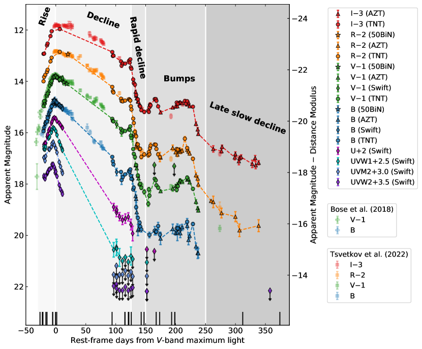
Figure 1: Multiband light curves of SN 2017egm. Our observations are obtained with the 50 cm Binocular Network (50BiN; stars), the AZT-22 1.5 m telescope (AZT; triangles), the Swift/Ultra-Violet/Optical Telescope (Swift, diamonds), and the Tsinghua-NAOC 0.80 m telescope (TNT; circles). The $BVRI$ photometry from literature [10, 15] (plus and squares) is overplotted for comparison. The error bars show 1$\sigma$ uncertainties. For visual clarity, photometric data presented in this work are connected with dashed lines. The multiple phases (rise, decline, rapid decline, bumps, and late-time slow decline) of the light curves are individually shaded and labelled. The vertical black lines indicate the epochs when spectroscopic observations are available (Supplementary Table 4). See Methods for details.

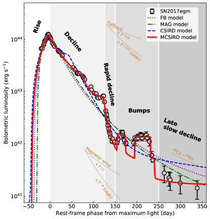
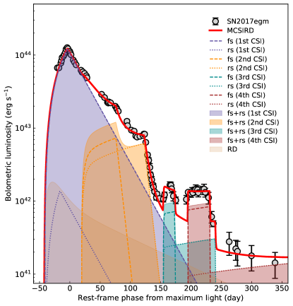
Figure 2: Model fits to the bolometric light curves of SN 2017egm. An MCSIRD model (red solid) can well explain the bolometric luminosity evolution of SN 2017egm (circles) by invoking four CSIs and ⁵⁶Ni decay (RD) as the power mechanisms. The error bars show 1$\sigma$ uncertainties. Left panel: the MCSIRD model (red) is compared with fallback-powered [50] (FB; purple dotted), magnetar-powered [12] (MAG; green dotted-dashed), and single CSIRD-powered [26] (CSIRD; blue dashed) models. The thin yellow solid lines (moved vertically for visual inspection) show the late-time input from the decay of ⁵⁶Co to ⁵⁶Fe, the fallback accretion ($\propto T^{-5/3}$ for no energy leakage and $\propto T^{-11/5}$ for full leakage), and the magnetar wind ($\propto T^{-2}$ for no energy leakage and $\propto T^{-4}$ for full leakage; here $T$ is the phase since explosion). The multiple phases of the light curve of this supernova (rise, decline, rapid decline, bumps, and late-time slow decline) of the light curves are individually grey-shaded and labelled. Right panel: for the MCSIRD model, the contributions from ⁵⁶Ni decay (yellow) and each CSI (purple, orange, green, red) are shown with shaded regions. The radiations powered by forward shock (fs) and reverse shock (rs) are shown in dashed and dotted lines, respectively.

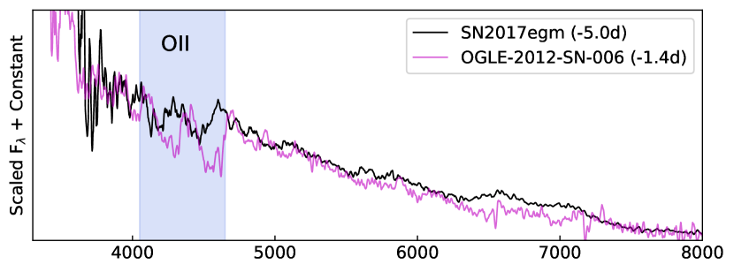
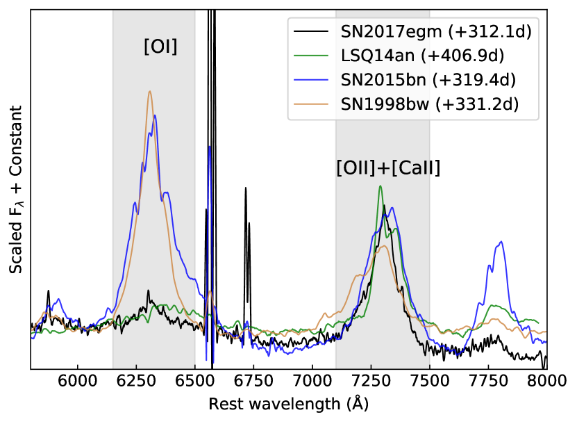
Figure 3: Spectral signs of powerful energy deposition for SN 2017egm. SN 2017egm shows early-time O ii absorption (upper panel) and late-time low line-intensity ratio of [O i]/([Ca ii] + [O ii] (lower panel). The comparison SNe include type Ibn supernova OGLE-2012-SN-006 (purple) [31], type Ic-BL supernova SN 1998bw (yellow) [51] and SLSNe-I (LSQ14an, green; SN 2015bn, blue) [38]. All of the spectra were smoothed with a Savitzky-Golay filter.

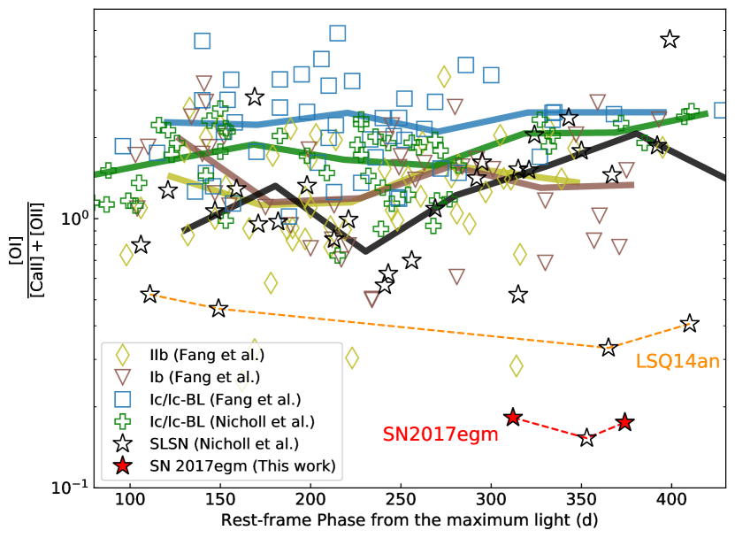
Figure 4: The nebular-phase [Oi]/([Caii] + [Oii]) ratios of SLSNe-I and other types of envelope-stripped supernovae. The measured flux ratios of SN 2017egm (red filled stars, this work) are compared with previous sample of SLSNe-I (empty stars), type IIb supernovae (yellow diamonds), type Ib supernovae (brown triangles) and type Ic/Ic-BL supernovae (blue squares and green pluses) [33, 34, 35, 16]. The LSQ14an and SN 2017egm data are connected with orange and red dashed lines, respectively. For each comparison sample, the corresponding solid line represents the average line ratios for bins of 50 or 100 days (each supernova contributes only one data point or one average value per bin). We caution that the [Oi] luminosity of SN 2017egm at $t\lesssim 250$ d could be overestimated owing to blends of multiple features around 6300 Å  (Extended Data Fig. 6, top left). Thus, the ratios measured during that period from Ref. [16] are not shown here.

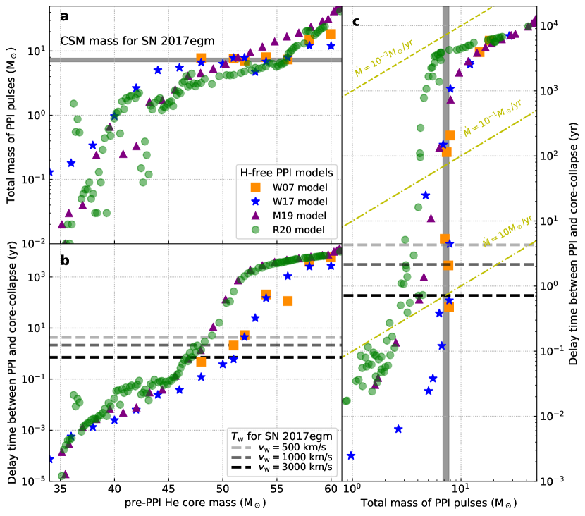
Figure 5: Comparison with hydrogen-free PPI models. The inferred properties of SN 2017egm are shown against four hydrogen-free PPI models of W07[42] (orange squares) , W17 [43] (blue stars), M19 [45] (purple triangles), and R20 [46] (green circles), in the diagrams of PPI-driven mass loss versus pre-pulsation helium core mass (a), delay time between the PPI onset and core-collaspe explosion versus pre-pulsation helium-core mass (b) and delay time versus PPI-driven mass loss (c). The narrow grey shade shows the total mass range (within 1$\sigma$ uncertainty) of four CSM shells inferred from light-curve modeling of SN 2017egm. Assuming velocities of $v_{w}=$ 500, 1000, 3000 km s^-1, the inferred delay times between core collapse and the eruption related to the outermost shell ($T_{\mathrm{w}}$) are displayed with gray dashed lines. The yellow lines represent the steady mass ejections with mass-loss rates of $\dot{M}=10^{-3},0.1,10$ M_⊙ yr ^-1.

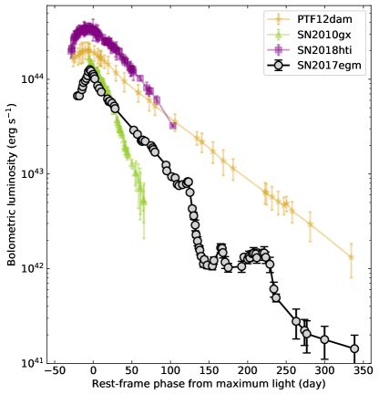
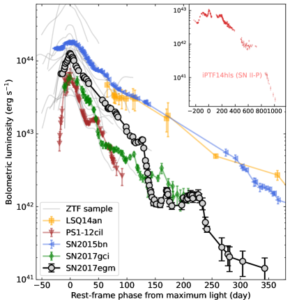
Extended Data Figure 1: The bolometric light curve of SN 2017egm, as compared to some representative SLSNe-I. Comparison SLSNe-I include objects with monotonic decay after maximum light (left panel: PTF12dam, yellow stars; SN 2010gx, yellow-green triangles; SN 2018hti, purple squares) and those with post-peak bumps (right panel: LSQ14an, orange squares; PS1-12cil, brown triangles; SN 2015bn, blue triangles; SN 2017gci, green diamonds; ZTF sample, gray lines). The bolometric luminosities of PTF12dam, SN 2017gci, SN 2018hti and ZTF sample are retrieved from the literatures[92, 93, 79, 18], while those of other comparison SLSNe-I are derived by fitting the UV-absorbed blackbody curve [12] to its multiband photometry [60, 94, 95, 96, 97, 98]. In the inset of the right panel, the luminosity evolution of a peculiar SN II iPTF14hls (red pluses) is shown for comparison [19, 88]. The error bars show 1$\sigma$ uncertainties.

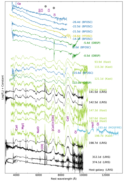
Extended Data Figure 2: Spectra of SN 2017egm and its host galaxy. The observations were obtained with Lick+Kast (yellow green), LJT+YFOSC (yellow), Keck+LRIS (black), Keck+MOSFIRE (light blue), P200+DBSP (green), and XLT+BFOSC (blue). All of the spectra were smoothed with a Savitzky-Golay filter. Telluric absorption that was not removed in some of the spectra is marked with an Earth symbol.

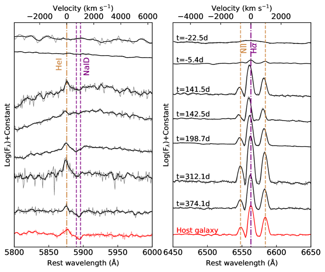
Extended Data Figure 3: Narrow spectral features observed in the spectra of SN 2017egm and its host galaxy. The spectra of SN and galaxy are displayed in black and red, respectively. Left panel: He i emission (yellow dot-dashed) and Na i D absorption (purple dashed). Right panel: [N ii] (yellow dashed) and H$\alpha$ (purple dot-dashed).

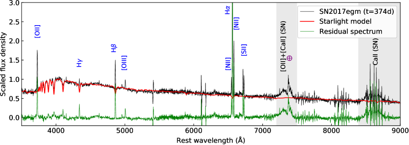
Extended Data Figure 4: Identification of emission lines from the host galaxy of SN 2017egm. The black line shows the Keck+LRIS spectrum obtained at the SN location on 2018 July 13, and the green line displays the residual spectrum after subtraction of the host-galaxy stellar component (red lines) obtained with a starlight-fitting tool [83]. The oxygen and calcium emission features from the SN are shown in gray shade. Incompletely removed telluric contamination is marked with an Earth symbol.

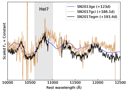
Extended Data Figure 5: Near-infrared (NIR) spectrum of SN 2017egm. The NIR spectra of superluminous SN 2017gci (yellow) [79] and Type Ic SN 2013ge (blue) [81] are overplotted for comparison. The prominent feature coincident with He i $\lambda$10,830 is shaded in gray. All spectra were smoothed with a Savitzky-Golay filter. See text for discussion.

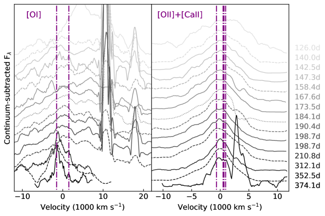
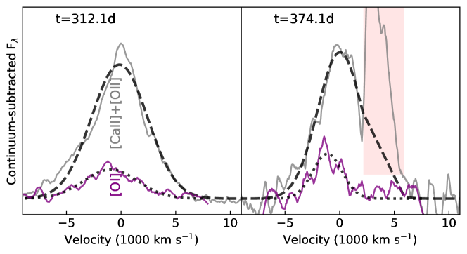
Extended Data Figure 6: Close-up view of the [Oi] $\lambda\lambda$6300, 6364 and [O ii] $\lambda\lambda$7319, 7330 + [Caii] $\lambda\lambda$7291, 7323 features in late-time spectra of SN 2017egm. Upper panel: observations of [Oi] (left) and [O ii] + [Caii] (right) features during the interval $t=126$–374 d are shown with dashed [16], dotted [69] and solid (this work) lines, respectively. The rest-frame wavelengths of these spectral lines are indicated by vertical dot-dashed lines. The 6300 Å  feature at $t=120$–210 d appears to be asymmetric about the rest wavelengths of [Oi], possibly owing to blends with other absorption or emission features. Lower panel: the photometry-calibrated profiles of [Oi] (purple) and [O ii] + [Caii] (gray) at $t=312$ d and $t=374$ d can be well fitted with Gaussian functions, as indicated by the dotted and dashed profiles, respectively. The spectral coverage contaminated by the incompletely removed telluric line is shaded in red and excluded from the Gaussian fit. All spectra were smoothed with the Savitzky-Golay filter.

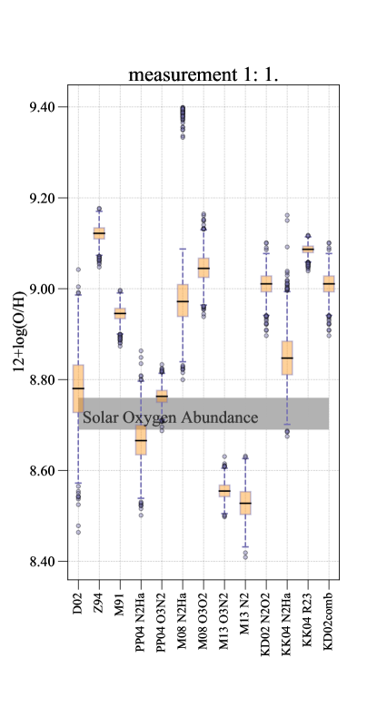
Extended Data Figure 7: Environmental metallicity of SN 2017egm estimated from different line-ratio diagnostics via the PYMCZ code [99]. For each diagnostic, we perform 2000 Monte Carlo sampling to obtain the median (black solid line) and interquartile range (IQR; orange box) of the metallicity distribution; the distribution spanning the range of $1.5\times$ IQR is represented by blue dashed lines (whisker), beyond which the sampling points are considered to be outliers; the minima and maxima values are shown by horizontal blue lines. The gray-shaded region shows the range of solar oxygen abundances reported in the literature.

Extended Data Table 1: Fitting Parameters of MCSIRD Model for SN 2017egm. Here $t_{\mathrm{exp}}$ is the explosion date from maximum light; $x_{0}$ is the dimensionless transitional radius between inner and outer part of ejecta; $E_{\mathrm{SN}}$ and $M_{\mathrm{ej}}$ are the kinetic energy and mass of the SN ejecta; $M_{\mathrm{Ni}}$ is the newly-synthesised ⁵⁶Ni mass; $t_{i,k}$ is the initial time of $k$-th interaction; $M_{\mathrm{CSM,k}}$ is the mass of $k$-th CSM shell, $\rho_{\mathrm{in,k}}$ is the CSM density at the inner radius ($R_{\mathrm{in,k}}$), and $\varepsilon_{\mathrm{fs},k}$ and $\varepsilon_{\mathrm{rs},k}$ are the efficiencies of converting forward and reverse shock energy to radiation. Here the subscript $k$ ($=1,2,3,4$) denotes the sequential number of CSM shell.

SN ejecta
$t_{\mathrm{exp}}$	$x_{0}$	$E_{\mathrm{SN}}$	$M_{\mathrm{ej}}$	$M_{\mathrm{Ni}}$
(day)		($10^{51}$ erg)	($M_{\odot}$)	($M_{\odot}$)
$-42.7_{-0.6}^{+0.4}$	$0.74_{-0.03}^{+0.03}$	$0.876_{-0.018}^{+0.025}$	$2.55_{-0.28}^{+0.38}$	$0.07_{-0.03}^{+0.04}$
1st CSM shell
$M_{\mathrm{CSM,1}}$	$R_{\mathrm{in,1}}$	$\rho_{\mathrm{in,1}}$	$\varepsilon_{\mathrm{fs},1}$	$\varepsilon_{\mathrm{rs},1}$
($M_{\odot}$)	($10^{15}$ cm)	($10^{-14}$ g cm-3)
$4.09_{-0.25}^{+0.23}$	$0.087_{-0.033}^{+0.037}$	$26.1_{-1.9}^{+2}$	$0.559_{-0.063}^{+0.095}$	$0.083_{-0.059}^{+0.119}$
2nd CSM shell
$M_{\mathrm{CSM,2}}$	$t_{i,2}$	$\rho_{\mathrm{in,2}}$	$\varepsilon_{\mathrm{fs},2}$	$\varepsilon_{\mathrm{rs},2}$
($M_{\odot}$)	(day)	($10^{-14}$ g cm-3)
$1.23_{-0.04}^{+0.05}$	$19.1_{-0.4}^{+0.6}$	$13.7_{-1.1}^{+1.2}$	$0.194_{-0.017}^{+0.019}$	$0.955_{-0.057}^{+0.032}$
3rd CSM shell
$M_{\mathrm{CSM,3}}$	$t_{i,3}$	$\rho_{\mathrm{in,3}}$	$\varepsilon_{\mathrm{fs},3}$	$\varepsilon_{\mathrm{rs},3}$
($M_{\odot}$)	(day)	($10^{-14}$ g cm-3)
$0.85_{-0.07}^{+0.07}$	$154_{-0.2}^{+0.2}$	$50.5_{-7.6}^{+7.7}$	$0.01$	$0.027_{-0.006}^{+0.006}$
4th CSM shell
$M_{\mathrm{CSM,4}}$	$t_{i,4}$	$\rho_{\mathrm{in,4}}$	$\varepsilon_{\mathrm{fs},4}$	$\varepsilon_{\mathrm{rs},4}$
($M_{\odot}$)	(day)	($10^{-14}$ g cm-3)
$1.1_{-0.1}^{+0.1}$	$194_{-0.6}^{+0.4}$	$6.4_{-3}^{+4.8}$	$0.041_{-0.012}^{+0.02}$	$0.038_{-0.014}^{+0.02}$

3 Supplementary Material

Supplementary Table 1: Reference stars used for photometry calibration. The numbers in brackets are $1\sigma$ uncertainties.

Star	$\alpha$(J2000)	$\delta$(J2000)	$B$ (mag)	$V$ (mag)	$R$ (mag)	$I$ (mag)
1	$10^{\rm hr}18^{\rm m}44.11^{\rm s}$	$46^{\circ}25^{\prime}1.33^{\prime\prime}$	14.759(0.035)	14.092(0.013)	13.698(0.015)	13.312(0.016)
2	10 18 44.99	46 32 11.98	19.257(0.037)	17.748(0.015)	16.896(0.016)	15.755(0.016)
3	10 18 53.4	46 23 41.25	19.868(0.057)	18.312(0.019)	17.435(0.015)	16.013(0.016)
4	10 18 55.41	46 22 48.51	16.085(0.039)	15.053(0.014)	14.461(0.016)	13.917(0.016)
5	10 18 58.5	46 23 08.08	17.469(0.034)	16.667(0.012)	16.199(0.016)	15.784(0.016)
6	10 19 0.11	46 27 20.11	19.177(0.035)	18.214(0.013)	17.659(0.015)	17.164(0.016)
7	10 19 0.52	46 25 01.75	18.007(0.036)	16.537(0.013)	15.706(0.015)	14.816(0.016)
8	10 19 13.21	46 30 59.5	17.761(0.034)	16.23(0.016)	15.366(0.017)	14.197(0.017)
9	10 19 20.64	46 31 24.98	16.365(0.034)	15.971(0.014)	15.725(0.016)	15.433(0.017)
10	10 19 26.18	46 24 04.76	19.73(0.036)	18.177(0.014)	17.302(0.016)	16.048(0.017)

Supplementary Table 2: $BVRI$ Photometry of SN 2017egm. The numbers in brackets are $1\sigma$ uncertainties in units of 0.001 mag.

MJD	$B$ (mag)	$V$ (mag)	$R$ (mag)	$I$ (mag)	Telescope
57905.56	15.941(31)	15.969(23)	15.997(31)	15.928(25)	TNT
57906.56	–	15.773(20)	15.830(20)	15.922(24)	TNT
57908.53	–	–	15.748(12)	–	TNT
57911.54	15.566(23)	15.552(18)	15.632(34)	15.598(13)	TNT
57911.65	15.551(27)	15.546(4)	–	–	50BiN
57912.56	15.425(28)	15.477(10)	15.551(24)	15.527(14)	TNT
57913.58	15.359(196)	15.449(11)	–	–	50BiN
57917.53	15.139(19)	15.045(23)	15.220(27)	15.237(19)	TNT
57919.54	14.974(20)	14.992(9)	15.078(22)	15.048(10)	TNT
57923.61	14.732(7)	14.829(6)	–	–	50BiN
57924.58	14.720(44)	14.842(6)	–	–	50BiN
57925.6	14.872(147)	14.806(13)	–	–	50BiN
57926.61	14.820(110)	14.806(7)	–	–	50BiN
57927.62	14.875(15)	14.818(18)	–	–	50BiN
57929.59	14.911(20)	14.848(28)	–	–	50BiN
57933.55	–	14.931(46)	14.849(26)	14.965(44)	TNT
57933.59	14.922(36)	14.933(20)	–	–	50BiN
57940.59	–	15.038(105)	–	–	50BiN
57945.58	14.914(43)	15.100(22)	–	–	50BiN
57946.57	15.017(43)	–	–	–	50BiN
57947.58	–	–	14.945(17)	–	50BiN
58023.86	16.943(23)	16.459(17)	16.218(29)	15.857(18)	TNT
58024.87	17.111(39)	16.543(16)	16.384(28)	16.011(26)	TNT
58025.87	17.233(60)	16.561(24)	16.434(36)	15.998(32)	TNT
58038.88	17.528(43)	16.853(19)	16.675(30)	16.225(24)	TNT
58039.88	17.844(175)	16.992(141)	16.768(41)	16.385(70)	TNT
58041.87	17.731(52)	16.912(14)	16.780(32)	16.301(22)	TNT
58045.88	17.623(29)	16.934(12)	16.750(29)	16.311(15)	TNT
58052.86	17.482(28)	16.860(16)	16.694(28)	16.193(15)	TNT
58053.89	17.523(53)	16.893(21)	16.725(33)	16.268(19)	TNT
58054.87	17.428(28)	16.753(18)	16.749(32)	16.142(20)	TNT
58055.87	17.676(23)	17.114(12)	16.971(30)	16.457(16)	TNT
58056.81	17.803(25)	17.209(22)	17.098(30)	16.512(19)	TNT
58059.87	18.212(51)	17.637(30)	17.452(42)	16.926(26)	TNT
58060.86	18.140(67)	17.824(48)	17.622(48)	17.068(30)	TNT
58062.9	–	17.951(85)	17.968(85)	17.128(62)	TNT
58064.02	18.468(173)	18.265(63)	18.024(108)	17.399(54)	AZT
58064.9	18.903(90)	18.257(46)	18.142(61)	17.533(55)	TNT
58065.01	18.576(143)	18.260(41)	18.532(118)	17.551(74)	AZT
58065.99	19.096(165)	18.387(21)	18.434(64)	17.658(33)	AZT
58067.89	19.319(74)	18.665(56)	18.457(46)	17.701(32)	TNT
58068.04	19.791(219)	18.672(25)	18.489(73)	17.774(59)	AZT
58069.03	19.736(86)	18.777(59)	18.538(78)	17.794(35)	AZT
58070.84	19.504(71)	19.021(50)	18.641(51)	17.948(42)	TNT
58071.84	19.653(89)	18.987(51)	18.627(59)	17.979(53)	TNT
58073.82	19.767(105)	19.146(67)	18.945(75)	18.122(58)	TNT
58078.89	–	19.307(90)	18.846(78)	18.187(62)	TNT
58085.82	–	19.773(99)	18.878(75)	18.139(53)	TNT
58086.76	–	19.209(75)	18.760(86)	18.187(61)	TNT
58087.8	19.983(108)	19.452(70)	18.842(65)	18.007(38)	TNT
58088.77	–	–	18.600(113)	17.913(76)	TNT
58089.79	–	–	18.503(103)	17.937(74)	TNT
58096.91	19.818(162)	18.796(50)	18.462(58)	17.691(29)	TNT
58098.74	19.865(118)	18.854(46)	18.469(53)	17.690(30)	TNT
58099.81	19.854(76)	19.049(38)	18.633(57)	17.759(26)	TNT
58102.79	19.636(142)	19.141(65)	18.844(54)	17.976(45)	TNT
58105.83	19.970(98)	–	18.948(182)	–	TNT
58106.95	20.123(236)	19.277(48)	18.966(70)	18.208(56)	AZT
58127.9	19.749(187)	19.174(106)	18.594(111)	18.016(40)	AZT
58132.99	19.904(88)	19.074(59)	18.756(76)	17.981(52)	AZT
58134.75	19.722(94)	19.224(78)	18.637(52)	17.827(39)	TNT
58135.88	19.880(325)	19.039(89)	18.849(86)	17.971(43)	AZT
58136.71	19.730(67)	19.086(40)	18.658(52)	17.879(38)	TNT
58138.95	19.717(81)	18.931(39)	18.704(86)	17.845(67)	AZT
58139.92	19.756(158)	18.860(48)	18.664(76)	17.819(31)	AZT
58140.93	19.915(173)	18.853(48)	18.742(76)	17.815(23)	AZT
58143.85	19.680(111)	18.899(46)	18.698(75)	17.849(35)	AZT
58148.78	–	–	18.233(83)	17.766(61)	TNT
58150.8	–	–	–	17.868(64)	TNT
58152.72	19.470(126)	18.751(67)	18.598(54)	17.772(33)	TNT
58152.92	19.628(92)	18.828(39)	18.663(69)	17.897(59)	AZT
58155.01	20.176(191)	18.796(46)	18.731(76)	17.817(21)	AZT
58156.99	20.013(117)	18.932(31)	18.806(74)	17.968(28)	AZT
58162.65	19.557(59)	19.186(51)	19.016(59)	17.988(40)	TNT
58167.9	20.428(127)	19.688(83)	19.655(96)	18.653(73)	AZT
58170.9	20.681(221)	19.941(54)	19.785(107)	18.870(72)	AZT
58171.88	20.696(182)	20.028(61)	20.014(101)	19.046(44)	AZT
58193.9	–	–	20.657(34)	–	AZT
58197.69	–	–	20.697(224)	19.632(123)	AZT
58211.81	–	–	21.130(190)	19.717(78)	AZT
58212.76	–	–	–	19.547(62)	AZT
58234.69	–	–	–	19.961(99)	AZT
58235.7	–	–	21.271(196)	19.832(85)	AZT
58241.73	–	–	–	20.109(141)	AZT
58242.79	–	–	21.802(246)	19.991(85)	AZT
58245.68	–	–	–	19.949(85)	AZT
58264.74	–	–	–	20.216(144)	AZT
58269.71	–	–	–	19.986(98)	AZT
58270.67	–	–	–	20.268(136)	AZT
58275.72	–	–	21.623(231)	20.170(81)	AZT

Supplementary Table 2: continued.

Supplementary Table 3: Swift Photometry of SN 2017egm. The numbers in brackets are $1\sigma$ uncertainties in units of 0.001 mag.

MJD	$UVW2$ (mag)	$UVM2$ (mag)	$UVW1$ (mag)	$U$ (mag)	$B$ (mag)	$V$ (mag)
57906.3	14.239(46)	13.972(46)	14.133(46)	14.461(56)	15.875(72)	15.891(104)
57906.4	14.172(47)	13.965(49)	14.040(46)	–	15.803(77)	15.877(119)
57908.2	14.299(56)	14.092(58)	14.144(54)	14.399(50)	15.629(72)	15.862(156)
57909.1	14.185(50)	13.917(50)	14.048(49)	14.421(50)	15.624(72)	15.764(132)
57912.1	14.088(60)	–	–	14.158(50)	–	–
57912.4	14.059(59)	–	–	14.140(50)	–	–
57912.7	–	–	–	14.067(48)	–	–
57912.8	14.034(59)	–	–	–	–	–
57914.5	13.943(52)	13.636(51)	13.707(50)	13.912(50)	15.258(68)	15.407(99)
57916.0	13.924(49)	13.650(49)	13.664(48)	13.850(48)	15.191(63)	15.161(74)
57919.2	13.865(49)	13.549(48)	13.485(46)	13.626(46)	14.962(58)	15.090(73)
57920.3	13.734(47)	13.420(46)	13.368(45)	13.562(46)	14.969(61)	14.945(70)
57922.2	13.731(47)	13.363(46)	13.303(45)	13.449(45)	14.790(55)	14.834(68)
57924.2	13.842(48)	13.475(47)	13.342(45)	13.416(44)	14.750(54)	14.828(67)
57925.7	13.946(52)	–	–	–	–	–
57926.7	14.016(51)	13.606(49)	13.434(46)	13.448(45)	14.804(56)	14.786(68)
57928.7	14.198(53)	13.771(50)	13.588(47)	13.548(46)	14.825(56)	14.845(68)
57932.6	14.538(59)	14.147(56)	13.853(50)	13.623(46)	14.921(57)	14.941(70)
57934.7	–	–	13.981(51)	–	–	–
57934.8	14.704(63)	14.320(60)	–	13.695(47)	14.972(59)	14.892(68)
57937.4	14.813(68)	14.504(61)	14.123(54)	13.780(48)	14.995(59)	14.941(72)
57938.1	14.890(71)	14.581(62)	14.188(56)	13.816(48)	15.071(64)	14.869(71)
58026.3	>18.471	>18.532	18.061(283)	16.898(143)	–	–
58031.0	>18.399	>18.185	17.962(313)	17.103(172)	–	–
58031.4	>18.568	>18.626	18.017(276)	17.011(149)	17.532(143)	16.676(141)
58036.3	>18.647	>18.537	18.361(350)	17.271(161)	–	–
58041.4	>18.644	>18.522	>18.493	17.403(178)	–	–
58046.3	>18.51	>18.377	>18.357	17.347(183)	–	–
58051.4	>18.651	>18.572	>18.536	17.279(160)	–	–
58056.0	>18.581	>18.426	18.304(354)	17.578(210)	–	–
58058.9	>18.535	>18.6	>18.422	17.926(288)	17.817(180)	17.156(204)
58083.4	>18.68	>18.588	>18.55	>18.544	–	–
58096.3	–	–	–	>18.619	–	>18.261
58130.5	–	–	–	–	–	>18.303
58295.3	>18.656	–	–	–	–	–

Supplementary Table 4: Journal of Spectroscopic Observations of SN 2017egm.

UT	MJD	Phasea	Instrument	Exp. time (s)	Range (Å)
2017-05-26	57899.5	$-$26.4	XLT/BFOSC	2700	3721–8781
2017-05-30	57903.6	$-$22.5	XLT/BFOSC	3000	3721–8794
2017-05-31	57904.5	$-$21.5	XLT/BFOSC	3000	3724–8793
2017-06-05	57909.6	$-$16.6	LJT/YFOSC	1600	3501–9170
2017-06-07	57911.6	$-$14.7	XLT/BFOSC	3000	3711–8780
2017-06-17	57921.1	$-$5.4	P200/DBSP	600	3800–10,000
2017-06-17	57921.5	$-$5	XLT/BFOSC	2700	3715–8660
2017-06-22	57926.2	$-0.5$	P200/DBSP	600	3800–10,000
2017-09-27	58023.5	93.9	Lick-3m/Kast	2130	3630–10,680
2017-10-19	58045.5	115.3	Lick-3m/Kast	1230	3622–10,670
2017-10-19	58045.9	115.6	XLT/BFOSC	3000	3730–8822
2017-10-25	58051.5	121.1	Lick-3m/Kast	2130	3620–10,680
2017-10-26	58052.4	122	P200/DBSP	1200	3500–9000
2017-10-30	58056.5	126	Lick-3m/Kast	3030	3622–10,712
2017-11-15	58072.6	141.5	Keck-I/LRIS	900	3072–10,293
2017-11-16	58073.6	142.5	Keck-I/LRIS	1165	3132–10,238
2017-11-21	58078.5	147.4	Lick-3m/Kast	2010	3632–10,710
2017-12-12	58099.5	167.5	Lick-3m/Kast	3630	3630–10,680
2017-12-18	58105.5	173.5	Lick-3m/Kast	3630	3632–10,716
2018-01-08	58126	193.4	Keck-I/MOSFIRE	1074	9751–11,240
2018-01-08	58126	193.4	Keck-I/MOSFIRE	954	11,530–13,518
2018-01-13	58131.5	198.7	Lick-3m/Kast	3630	3630–10,680
2018-01-13	58131.5	198.7	Keck-I/LRIS	1760	3066–10,264
2018-05-10	58248.4	312.1	Keck-I/LRIS	1757	3149–10,237
2018-07-13	58312.3	374.1	Keck-I/LRIS	2550	3099–10,287
host galaxy
2018-01-13	58131.5	198.7	Keck-I/LRIS	1760	3066–10,264

^aRest-frame days with respect to the epoch of maximum $V$ brightness.

Supplementary Table 5: Free Parameters and priors of the MCSIRD Model. Here $t_{\mathrm{exp}}$ is the explosion date from the maximum light; $x_{0}$ is the dimensionless transitional radius between inner and outer part of ejecta; $E_{\mathrm{SN}}$ and $M_{\mathrm{ej}}$ are the kinetic energy and mass of the SN ejecta; $M_{\mathrm{Ni}}$ is the newly-synthesised ⁵⁶Ni mass; $t_{i,k}$ is the initial time of $k$-th interaction; $M_{\mathrm{CSM,k}}$ is the mass of $k$-th CSM shell, $\rho_{\mathrm{in,k}}$ is the CSM density at the inner radius ($R_{\mathrm{in,k}}$), and $\varepsilon_{\mathrm{fs},k}$ and $\varepsilon_{\mathrm{rs},k}$ are the efficiencies of converting forward and reverse shock energy to radiation. Here the subscript $k$ ($=1,2,3,4$) denotes the sequential number of CSM shell.

Parameter	Unit	Prior	Min	Max
$t_{\mathrm{exp}}$	day	Flat	-100	-32
$x_{0}$	–	Flat	$0.1$	$1$
$E_{\mathrm{SN},1}$	$10^{51}$ erg	Log-Flat	$0.01$	$100$
$M_{\mathrm{ej},1}$	$M_{\odot}$	Log-Flat	0.01	100
$M_{\mathrm{Ni}}$	$M_{\odot}$	Log-Flat	0	10
$R_{\mathrm{in,1}}$	$10^{15}$ cm	Log-Flat	0.0001	1000
$t_{i,2}$	day	Flat	0	123
$t_{i,3}$	day	Flat	123	167
$t_{i,4}$	day	Flat	167	219
$M_{\mathrm{CSM,k}}$	$M_{\odot}$	Log-Flat	0.01	100
$\rho_{\mathrm{in,k}}$	$10^{-14}$ g cm-3	Log-Flat	0.0001	10000
$\varepsilon_{\mathrm{fs},k}$	–	Log-Flat	0.01	1
$\varepsilon_{\mathrm{rs},k}$	–	Log-Flat	0.01	1

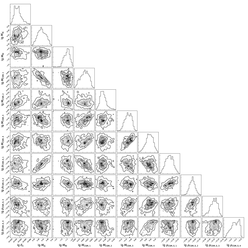
Supplementary Figure 1: Posteriors for some key parameters inferred for SN 2017egm using the MCSIRD model. The mean and $1\sigma$ uncertainties of fitting parameters are presented in Extended Data Table 1.

References

- [1] Quimby, R. M. et al. Hydrogen-poor superluminous stellar explosions. Nature 474, 487–489 (2011).
- [2] Gal-Yam, A. Luminous Supernovae. Science 337, 927–932 (2012).
- [3] Delgado, A. et al. GaiaAlerts Transient Discovery Report for 2017-05-25. Transient Name Server Discovery Report 2017-591, 1 (2017).
- [4] Lunnan, R. et al. Hydrogen-poor Superluminous Supernovae and Long-duration Gamma-Ray Bursts Have Similar Host Galaxies. Astrophys. J. 787, 138 (2014).
- [5] Leloudas, G. et al. Spectroscopy of superluminous supernova host galaxies. A preference of hydrogen-poor events for extreme emission line galaxies. Mon. Not. R. Astron. Soc. 449, 917–932 (2015).
- [6] Perley, D. A. et al. Host-galaxy Properties of 32 Low-redshift Superluminous Supernovae from the Palomar Transient Factory. Astrophys. J. 830, 13 (2016).
- [7] Izzo, L. et al. The host of the Type I SLSN 2017egm. A young, sub-solar metallicity environment in a massive spiral galaxy. Astron. Astrophys. 610, A11 (2018).
- [8] Chen, T.-W. et al. Spatially Resolved MaNGA Observations of the Host Galaxy of Superluminous Supernova 2017egm. Astrophys. J. Lett. 849, L4 (2017).
- [9] Nicholl, M. et al. The Superluminous Supernova SN 2017egm in the Nearby Galaxy NGC 3191: A Metal-rich Environment Can Support a Typical SLSN Evolution. Astrophys. J. Lett. 845, L8 (2017).
- [10] Bose, S. et al. Gaia17biu/SN 2017egm in NGC 3191: The Closest Hydrogen-poor Superluminous Supernova to Date Is in a “Normal,” Massive, Metal-rich Spiral Galaxy. Astrophys. J. 853, 57 (2018).
- [11] Yan, L. et al. Far-UV HST Spectroscopy of an Unusual Hydrogen-poor Superluminous Supernova: SN2017egm. Astrophys. J. 858, 91 (2018).
- [12] Nicholl, M., Guillochon, J. & Berger, E. The Magnetar Model for Type I Superluminous Supernovae. I. Bayesian Analysis of the Full Multicolor Light-curve Sample with MOSFiT. Astrophys. J. 850, 55 (2017).
- [13] Wheeler, J. C., Chatzopoulos, E., Vinkó, J. & Tuminello, R. Circumstellar Interaction Models for the Bolometric Light Curve of Type I Superluminous SN 2017egm. Astrophys. J. Lett. 851, L14 (2017).
- [14] Hosseinzadeh, G. et al. Bumpy Declining Light Curves Are Common in Hydrogen-poor Superluminous Supernovae. Astrophys. J. 933, 14 (2022).
- [15] Tsvetkov, D. Y. et al. Photometric observations of SN 2017egm and peculiar transient AT 2018cow. Contributions of the Astronomical Observatory Skalnate Pleso 52, 46–63 (2022).
- [16] Nicholl, M., Berger, E., Blanchard, P. K., Gomez, S. & Chornock, R. Nebular-phase Spectra of Superluminous Supernovae: Physical Insights from Observational and Statistical Properties. Astrophys. J. 871, 102 (2019).
- [17] Coppejans, D. L. et al. Jets in Hydrogen-poor Superluminous Supernovae: Constraints from a Comprehensive Analysis of Radio Observations. Astrophys. J. 856, 56 (2018).
- [18] Chen, Z. H. et al. The Hydrogen-poor Superluminous Supernovae from the Zwicky Transient Facility Phase I Survey. II. Light-curve Modeling and Characterization of Undulations. Astrophys. J. 943, 42 (2023).
- [19] Arcavi, I. et al. Energetic eruptions leading to a peculiar hydrogen-rich explosion of a massive star. Nature 551, 210–213 (2017).
- [20] Moriya, T. J., Murase, K., Kashiyama, K. & Blinnikov, S. I. Variable thermal energy injection from magnetar spin-down as a possible cause of stripped-envelope supernova light-curve bumps. Mon. Not. R. Astron. Soc. 513, 6210–6218 (2022).
- [21] Metzger, B. D., Beniamini, P. & Giannios, D. Effects of Fallback Accretion on Protomagnetar Outflows in Gamma-Ray Bursts and Superluminous Supernovae. Astrophys. J. 857, 95 (2018).
- [22] Lin, W., Wang, X., Wang, L. & Dai, Z. Supernova Luminosity Powered by Magnetar-Disk System. Astrophys. J. Lett. 914, L2 (2021).
- [23] Yan, L. et al. Detection of Broad H Emission Lines in the Late-time Spectra of a Hydrogen-poor Superluminous Supernova. Astrophys. J. 814, 108 (2015).
- [24] Yan, L. et al. Hydrogen-poor Superluminous Supernovae with Late-time H Emission: Three Events From the Intermediate Palomar Transient Factory. Astrophys. J. 848, 6 (2017).
- [25] Sun, L., Xiao, L. & Li, G. A mid-infrared study of superluminous supernovae. Mon. Not. R. Astron. Soc. 513, 4057–4073 (2022).
- [26] Chatzopoulos, E., Wheeler, J. C. & Vinko, J. Generalized Semi-analytical Models of Supernova Light Curves. Astrophys. J. 746, 121 (2012).
- [27] Gal-Yam, A. et al. A WC/WO star exploding within an expanding carbon-oxygen-neon nebula. Nature 601, 201–204 (2022).
- [28] Perley, D. A. et al. The Type Icn SN 2021csp: Implications for the Origins of the Fastest Supernovae and the Fates of Wolf-Rayet Stars. Astrophys. J. 927, 180 (2022).
- [29] Chatzopoulos, E., Wheeler, J. C., Vinko, J., Horvath, Z. L. & Nagy, A. Analytical Light Curve Models of Superluminous Supernovae: 2-minimization of Parameter Fits. Astrophys. J. 773, 76 (2013).
- [30] Ben-Ami, S. et al. SN 2010mb: Direct Evidence for a Supernova Interacting with a Large Amount of Hydrogen-free Circumstellar Material. Astrophys. J. 785, 37 (2014).
- [31] Pastorello, A. et al. Massive stars exploding in a He-rich circumstellar medium - V. Observations of the slow-evolving SN Ibn OGLE-2012-SN-006. Mon. Not. R. Astron. Soc. 449, 1941–1953 (2015).
- [32] Mazzali, P. A., Sullivan, M., Pian, E., Greiner, J. & Kann, D. A. Spectrum formation in superluminous supernovae (Type I). Mon. Not. R. Astron. Soc. 458, 3455–3465 (2016).
- [33] Fang, Q. & Maeda, K. The Origin of the Ha-like Structure in Nebular Spectra of Type IIb Supernovae. Astrophys. J. 864, 47 (2018).
- [34] Fang, Q., Maeda, K., Kuncarayakti, H., Sun, F. & Gal-Yam, A. A hybrid envelope-stripping mechanism for massive stars from supernova nebular spectroscopy. Nature Astronomy 3, 434–439 (2019).
- [35] Fang, Q. et al. Statistical Properties of the Nebular Spectra of 103 Stripped-envelope Core-collapse Supernovae. Astrophys. J. 928, 151 (2022).
- [36] Mösta, P. et al. A large-scale dynamo and magnetoturbulence in rapidly rotating core-collapse supernovae. Nature 528, 376–379 (2015).
- [37] Drout, M. R. et al. The First Systematic Study of Type Ibc Supernova Multi-band Light Curves. Astrophys. J. 741, 97 (2011).
- [38] Jerkstrand, A. et al. Long-duration Superluminous Supernovae at Late Times. Astrophys. J. 835, 13 (2017).
- [39] Dessart, L. Simulations of light curves and spectra for superluminous Type Ic supernovae powered by magnetars. Astron. Astrophys. 621, A141 (2019).
- [40] Chandra, P., Chevalier, R. A., Chugai, N., Fransson, C. & Soderberg, A. M. X-Ray and Radio Emission from Type IIn Supernova SN 2010jl. Astrophys. J. 810, 32 (2015).
- [41] Smith, N. Interacting Supernovae: Types IIn and Ibn, 403 (Handbook of Supernovae, Springer International Publishing, 2017).
- [42] Woosley, S. E., Blinnikov, S. & Heger, A. Pulsational pair instability as an explanation for the most luminous supernovae. Nature 450, 390–392 (2007).
- [43] Woosley, S. E. Pulsational Pair-instability Supernovae. Astrophys. J. 836, 244 (2017).
- [44] Chatzopoulos, E. & Wheeler, J. C. Hydrogen-poor Circumstellar Shells from Pulsational Pair-instability Supernovae with Rapidly Rotating Progenitors. Astrophys. J. 760, 154 (2012).
- [45] Marchant, P. et al. Pulsational Pair-instability Supernovae in Very Close Binaries. Astrophys. J. 882, 36 (2019).
- [46] Renzo, M. et al. Predictions for the hydrogen-free ejecta of pulsational pair-instability supernovae. Astron. Astrophys. 640, A56 (2020).
- [47] Abbott, B. P et al. GWTC-1: A Gravitational-Wave Transient Catalog of Compact Binary Mergers Observed by LIGO and Virgo during the First and Second Observing Runs. Phys. Rev. X 9, 031040 (2019).
- [48] Leung, S.-C., Nomoto, K. & Blinnikov, S. Pulsational Pair-instability Supernovae. I. Pre-collapse Evolution and Pulsational Mass Ejection. Astrophys. J. 887, 72 (2019).
- [49] Vigna-Gómez, A., Justham, S., Mandel, I., de Mink, S. E. & Podsiadlowski, P. Massive Stellar Mergers as Precursors of Hydrogen-rich Pulsational Pair Instability Supernovae. Astrophys. J. Lett. 876, L29 (2019).
- [50] Moriya, T. J., Nicholl, M. & Guillochon, J. Systematic Investigation of the Fallback Accretion-powered Model for Hydrogen-poor Superluminous Supernovae. Astrophys. J. 867, 113 (2018).
- [51] Patat, F. et al. The Metamorphosis of SN 1998bw. Astrophys. J. 555, 900–917 (2001).
- [52] Deng, L. et al. SONG China project - participating in the global network. in Proc. IAU Symp. 288, Astrophysics from Antarctica (eds Burton, M. G. et al.) 318 (Cambridge: Cambridge Univ. Press, 2013).
- [53] Ehgamberdiev, S. Modern astronomy at the Maidanak observatory in Uzbekistan. Nature Astronomy 2, 349–351 (2018).
- [54] Wang, X. et al. Optical and Near-Infrared Observations of the Highly Reddened, Rapidly Expanding Type Ia Supernova SN 2006X in M100. Astrophys. J. 675, 626–643 (2008).
- [55] Huang, F. et al. The photometric system of the Tsinghua-NAOC 80-cm telescope at NAOC Xinglong Observatory. Research in Astronomy and Astrophysics 12, 1585–1596 (2012).
- [56] Becker, A. HOTPANTS: High Order Transform of PSF ANd Template Subtraction. Astrophysics Source Code Library, record ascl:1504.004 (2015).
- [57] Tonry, J. L. et al. The Pan-STARRS1 Photometric System. Astrophys. J. 750, 99 (2012).
- [58] Magnier, E. A. et al. Pan-STARRS Photometric and Astrometric Calibration. Astrophys. J. Suppl. 251, 6 (2020).
- [59] Roming, P. W. A. et al. The Swift Ultra-Violet/Optical Telescope. Space Sci. Rev. 120, 95–142 (2005).
- [60] Brown, P. J., Breeveld, A. A., Holland, S., Kuin, P. & Pritchard, T. SOUSA: the Swift Optical/Ultraviolet Supernova Archive. Astron. Space Sci. 354, 89–96 (2014).
- [61] Breeveld, A. A. et al. An Updated Ultraviolet Calibration for the Swift/UVOT. AIP Conf. Proc., 1358, 373–376 (2011).
- [62] Virtanen, P. et al. SciPy 1.0: Fundamental Algorithms for Scientific Computing in Python. Nature Methods 17, 261–272 (2020).
- [63] Inserra, C. et al. Super-luminous Type Ic Supernovae: Catching a Magnetar by the Tail. Astrophys. J. 770, 128 (2013).
- [64] Schlafly, E. F. & Finkbeiner, D. P. Measuring Reddening with Sloan Digital Sky Survey Stellar Spectra and Recalibrating SFD. Astrophys. J. 737, 103 (2011).
- [65] Albareti, F. D. et al. The 13th Data Release of the Sloan Digital Sky Survey: First Spectroscopic Data from the SDSS-IV Survey Mapping Nearby Galaxies at Apache Point Observatory. Astrophys. J. Suppl. 233, 25 (2017).
- [66] Liu, L.-D., Wang, L.-J., Wang, S.-Q. & Dai, Z.-G. A Multiple Ejecta-circumstellar Medium Interaction Model and Its Implications for Superluminous Supernovae iPTF15esb and iPTF13dcc. Astrophys. J. 856, 59 (2018).
- [67] Chevalier, R. A. Self-similar solutions for the interaction of stellar ejecta with an external medium. Astrophys. J. 258, 790–797 (1982).
- [68] Maund, J. R., Steele, I., Jermak, H., Wheeler, J. C. & Wiersema, K. RINGO3 polarimetry of the Type I superluminous SN 2017egm. Mon. Not. R. Astron. Soc. 482, 4057–4061 (2019).
- [69] Saito, S. et al. Late-phase Spectropolarimetric Observations of Superluminous Supernova SN 2017egm to Probe the Geometry of the Inner Ejecta. Astrophys. J. 894, 154 (2020).
- [70] Shappee, B. J. et al. The Man behind the Curtain: X-Rays Drive the UV through NIR Variability in the 2013 Active Galactic Nucleus Outburst in NGC 2617. Astrophys. J. 788, 48 (2014).
- [71] Foreman-Mackey, D., Hogg, D. W., Lang, D. & Goodman, J. emcee: The MCMC Hammer. Publ. Astron. Soc. Pac. 125, 306 (2013).
- [72] Oke, J. B. & Gunn, J. E. An Efficient Low Resolution and Moderate Resolution Spectrograph for the Hale Telescope. Publ. Astron. Soc. Pac. 94, 586 (1982).
- [73] Fan, Y.-F. et al. Rapid instrument exchanging system for the Cassegrain focus of the Lijiang 2.4-m Telescope. Research in Astronomy and Astrophysics 15, 918 (2015).
- [74] Miller, J. & Stone, R. Lick Observatory Technical Reports Lick Obs. Santa Cruz, CA 66 (1993).
- [75] Oke, J. B. et al. The Keck Low-Resolution Imaging Spectrometer. Publ. Astron. Soc. Pac. 107, 375 (1995).
- [76] McLean, I. S. et al. MOSFIRE, the multi-object spectrometer for infra-red exploration at the Keck Observatory. Proc. SPIE 8446, 84460J (2012).
- [77] Filippenko, A. V. The importance of atmospheric differential refraction in spectrophotometry. Publ. Astron. Soc. Pac. 94, 715–721 (1982).
- [78] Zhu, J. et al. SN2017egm: A Helium-rich Superluminous Supernova with Multiple Bumps in the Light Curves. arXiv:2303.03424 (2023).
- [79] Fiore, A. et al. SN 2017gci: a nearby Type I Superluminous Supernova with a bumpy tail. Mon. Not. R. Astron. Soc. 502, 2120–2139 (2021).
- [80] Shahbandeh, M. et al. Carnegie Supernova Project-II: Near-infrared Spectroscopy of Stripped-envelope Core-collapse Supernovae. Astrophys. J. 925, 175 (2022).
- [81] Drout, M. R. et al. The Double-peaked SN 2013ge: A Type Ib/c SN with an Asymmetric Mass Ejection or an Extended Progenitor Envelope. Astrophys. J. 821, 57 (2016).
- [82] Poznanski, D., Prochaska, J. X. & Bloom, J. S. An empirical relation between sodium absorption and dust extinction. Mon. Not. R. Astron. Soc. 426, 1465–1474 (2012).
- [83] Cid Fernandes, R., Mateus, A., Sodré, L., Stasińska, G. & Gomes, J. M. Semi-empirical analysis of Sloan Digital Sky Survey galaxies - I. Spectral synthesis method. Mon. Not. R. Astron. Soc. 358, 363–378 (2005).
- [84] Asplund, M., Grevesse, N., Sauval, A. J. & Scott, P. The Chemical Composition of the Sun. Annu. Rev. Astron. Astrophys. 47, 481–522 (2009).
- [85] Schulze, S. et al. Cosmic evolution and metal aversion in superluminous supernova host galaxies. Mon. Not. R. Astron. Soc. 473, 1258–1285 (2018).
- [86] Schulze, S. et al. The Palomar Transient Factory Core-collapse Supernova Host-galaxy Sample. I. Host-galaxy Distribution Functions and Environment Dependence of Core-collapse Supernovae. Astrophys. J. Suppl. 255, 29 (2021).
- [87] Prentice, S. J. et al. The bolometric light curves and physical parameters of stripped-envelope supernovae. Mon. Not. R. Astron. Soc. 458, 2973–3002 (2016).
- [88] Sollerman, J. et al. Late-time observations of the extraordinary Type II supernova iPTF14hls. Astron. Astrophys. 621, A30 (2019).
- [89] Wang, L.-J. et al. iPTF14hls in the Circumstellar Medium Interaction Model: A Promising Candidate for a Pulsational Pair-instability Supernova. Astrophys. J. 933, 102 (2022).
- [90] Lin, W. L. et al. Photometric and spectroscopic dataset of superluminous supernova SN 2017egm. Figshare https://doi.org/10.6084/m9.figshare.22009868, (2023).
- [91] Yaron, O. & Gal-Yam, A. WISeREP—An Interactive Supernova Data Repository. Publ. Astron. Soc. Pac. 124, 668 (2012).
- [92] Vreeswijk, P. M. et al. On the Early-time Excess Emission in Hydrogen-poor Superluminous Supernovae. Astrophys. J. 835, 58 (2017).
- [93] Lin, W. L. et al. SN 2018hti: a nearby superluminous supernova discovered in a metal-poor galaxy. Mon. Not. R. Astron. Soc. 497, 318–335 (2020).
- [94] Nicholl, M. et al. SN 2015BN: A Detailed Multi-wavelength View of a Nearby Superluminous Supernova. Astrophys. J. 826, 39 (2016).
- [95] Nicholl, M. et al. Superluminous Supernova SN 2015bn in the Nebular Phase: Evidence for the Engine-powered Explosion of a Stripped Massive Star. Astrophys. J. Lett. 828, L18 (2016).
- [96] Inserra, C. et al. Complexity in the light curves and spectra of slow-evolving superluminous supernovae. Mon. Not. R. Astron. Soc. 468, 4642–4662 (2017).
- [97] De Cia, A. et al. Light Curves of Hydrogen-poor Superluminous Supernovae from the Palomar Transient Factory. Astrophys. J. 860, 100 (2018).
- [98] Lunnan, R. et al. Hydrogen-poor Superluminous Supernovae from the Pan-STARRS1 Medium Deep Survey. Astrophys. J. 852, 81 (2018).
- [99] Bianco, F. B. et al. Monte Carlo method for calculating oxygen abundances and their uncertainties from strong-line flux measurements. Astronomy and Computing 16, 54–66 (2016).