DNA-Correcting Codes: End-to-end Correction in DNA Storage Systems

Abstract

This paper introduces a new solution to DNA storage that integrates all three steps of retrieval, namely clustering, reconstruction, and error correction. DNA-correcting codes are presented as a unique solution to the problem of ensuring that the output of the storage system is unique for any valid set of input strands. To this end, we introduce a novel distance metric to capture the unique behavior of the DNA storage system and provide necessary and sufficient conditions for DNA-correcting codes. The paper also includes several upper bounds and constructions of DNA-correcting codes.

I Introduction

The first two experiments that showed the potential of using synthetic DNA as a means for a large-scale information storage system were done in[5] and[7]. Since then, together with the developments in synthesis and sequencing technologies, more research groups showed the potential of in vitro DNA storage; see e.g. [1, 2, 3, 4, 6, 11, 18, 19].

A typical DNA storage system consists of three components: (1) synthesizing the strands that contain the encoded data. In current technologists, each strand has millions of copies, and the length of these strands is usually limited to 250-300 nucleotides; (2) a storage container that stores the synthetic DNA strands; (3) a DNA sequencing that reads the strands, the output sequences from the sequencing machine are called reads. This novel technology has several properties that are fundamentally different from its digital counterparts, while the most prominent one is that the erroneous copies are stored in an unordered manner in the storage container (see e.g. [10]). The most common solution to overcome this challenge is to use indices that are stored as part of the strand. Each strand is prefixed with some nucleotides that indicate the strand’s location, with respect to all other strands, these indices are usually protected using an error-correcting code (ECC) [2], [3], [9], [11],[18]. The retrieval of the input information is usually done by the following three steps. The first step is to partition all the reads into clusters such that the reads at each cluster are all copies of the same information strand. The second step is applying a reconstruction algorithm on every cluster to retrieve an approximation of the original input strands. In the last step, an ECC is used in order to correct the remaining errors and retrieve the user’s information.

While previous works tackled each of these steps independently (see e.g. [1],[2], [3],[11], [17], [18]), this work aims to tackle all of them together. This is accomplished by limiting the stored messages in the DNA storage system, such that for any two input messages, the sets of all the possible outputs will be mutually disjoint, we call this family of codes DNA-correcting codes. Our point of departure is the recent work [16] of clustering-correcting codes that proposed codes for successful clustering. However, their results have been established under the assumption that the correct reads in every cluster satisfy some dominance property. Furthermore, the codes in [16] do not aim to recover the input data, but only to achieve a successful clustering. On the contrary, our suggested codes also guarantee the recovery of the input data, while eliminating the dominance assumption. Similar to [16], it is assumed that every information strand consists of an index-field and a data-field.

The rest of the paper is organized as follows. Section II presents the definitions and the problem statement. In Section III, we consider the case where the data-field is error-free. In addition, we present the DNA-distance metric, which is used in order to find necessary and sufficient conditions for DNA-correcting codes. In section IV, we study codes over the index-field. Using these codes we present constructions for DNA-correcting codes and bounds on the size of DNA-correcting codes. Lastly, several generalizations and open problems are discussed in Section V.

II Definitions, Problem Statement, and Related Works

The following notations will be used in this paper. For a positive integer $n$, the set $\{0,1,\dots,n-1\}$ is denoted by $[n]$ and $\{0,1\}^{n}$ is the set of all length-$n$ binary vectors. For two vectors ${\boldsymbol{x}},{\boldsymbol{y}},$ of the same length, the Hamming distance between them is the number of coordinates in which they differ and is denoted by $d_{H}({\boldsymbol{x}},{\boldsymbol{y}})$. For two sets of vectors of the same size $Z,Y$, let $BI(Z,Y)$ be the space of all bijective functions (matchings) from $Z$ to $Y$ and for a matching $\pi\in BI(Z,Y)$, let $w_{H}(\pi)$ denote the maximal Hamming distance between any two matched vectors, i.e., $w_{H}(\pi)=\max\limits_{{\boldsymbol{z}}\in Z}\{d_{H}({\boldsymbol{z}},\pi({\boldsymbol{z}}))\}$. We assume a binary alphabet in the paper as the generalization to higher alphabets will be immediate and all logs are taken according to base 2.

Assume that a set of $M$ unordered length-$L$ strands are stored in a DNA-based storage system. We will assume that $M=2^{\beta L}$ for some $0<\beta<1$, and for simplicity, it is assumed that $\beta L$ is an integer. Every stored length-$L$ strand ${\boldsymbol{s}}$ is of the form ${\boldsymbol{s}}=(ind,{\boldsymbol{u}})$, where $ind$ is the length-$\bf{\ell}$ index-field of the strand (which represents the relative position of this strand in relation to all other strands) and ${\boldsymbol{u}}$ is the length-$(L-\ell)$ data-field of the strand. Different strands are required to have a different index-field, as otherwise, it will not be possible to determine the order of the strands. The length of the index-field of all the strands is the same and since all indices are different it holds that $\ell$ $\geq\log(M)=\beta L$.

For $M,L$, and $\ell$, the space of all possible messages that can be stored in the DNA storage system is:

$$\mathcal{X}_{M,L,\ell}=\big{\{}\{ (ind_{1},{\boldsymbol{u}}_{1}),(ind_{2},{\boldsymbol{u}}_{2}),\dots,(ind_{M},{\boldsymbol{u}}_{M})\}|$$

$$\forall i:ind_{i}\in\{{0,1}\}^{\ell},{\boldsymbol{u}}_{i}\in\{0,1\}^{L-\ell},$$ (1)

$$\forall i\neq j:ind_{i}\neq ind_{j}\big{\}}.$$

Note that $|\mathcal{X}_{M,L,\ell}|={2^{\ell}\choose M}{2^{(L-\ell)M}}$ since there are $2^{\ell}\choose M$ options to choose the different set of index-fields and then $2^{(L-\ell)M}$ more options to choose the data-field for every index. Under this setup, a code $\mathcal{C}$ will be a subset of $\mathcal{X}_{M,L,\ell}$.

When a set $Z=\{(ind_{1},{\boldsymbol{u}}_{1}),\dots,(ind_{M},{\boldsymbol{u}}_{M})\}$ is synthesized, each of its strands has a large number of noisy copies, and during the sequencing process a subset of these copies is read, while the number of copies mostly depends on the synthesis and sequencing technologies. Throughout this paper, it is assumed that the number of copies for each strand is exactly $K$, and so, the sequencer’s output is a set of $MK$ reads, where every output read is a noisy copy of one of the input strands. It is also assumed that the noise is of substitution type and in Section V we explain how most of the results hold for edit errors as well when changing the Hamming distance to edit. Let $\tau$ denote the maximal relative fraction of incorrect copies that every input strand can have and by $e_{i},e_{d}$ the largest number of errors that can occur at the index, data-field of each strand, respectively. Formally, the DNA storage channel is modeled as follows.

Definition 1.

A DNA-based storage system is called a $(\tau,e_{i},e_{d})_{K}$-DNA storage system if it satisfies the following properties: (1) Every input strand $(ind,{\boldsymbol{u}})$ has exactly $K$ output copies, (2) at most $\lfloor\tau K\rfloor$ of these copies are erroneous, and (3) if $(ind^{\prime},{\boldsymbol{u}}^{\prime})$ is a noisy copy of $(ind,{\boldsymbol{u}})$ then $d_{H}(ind,ind^{\prime})\leq e_{i}$ and $d_{H}({\boldsymbol{u}},{\boldsymbol{u}}^{\prime})\leq e_{d}$.

For a set $Z\in\mathcal{X}_{M,L,\ell}$, let $B^{K}_{(\tau,e_{i},e_{d})}(Z)$ be the set of all possible $MK$ reads one can get from $Z$ after it passes through a $(\tau,e_{i},e_{d})_{K}$-DNA storage system (i.e., every element in $B^{K}_{(\tau,e_{i},e_{d})}(Z)$ is a multiset of $MK$ reads). Under this setup, a code $\mathcal{C}\subseteq\mathcal{X}_{M,L,\ell}$ is called a $(\tau,e_{i},e_{d})_{K}$-DNA-correcting code if for every two codewords $Z,Z^{\prime}\in\mathcal{C}$ such that $Z\neq Z^{\prime}$, it holds that $B^{K}_{(\tau,e_{i},e_{d})}(Z)\cap B^{K}_{(\tau,e_{i},e_{d})}(Z^{\prime})=\emptyset$, i.e., the sets of possible outputs for all codewords are mutually disjoint when the parameters are $\tau,e_{i},e_{d}$ and $K$. The redundancy of such a code is defined by $r(\mathcal{C})=\log_{2}(|\mathcal{X}_{M,L,\ell}|)-\log_{2}(|\mathcal{C}|)$.

Let $A_{M,L,\ell}(\tau,e_{i},e_{d},K)$ denote the size of a largest $(\tau,e_{i},e_{d})_{K}$-DNA-correcting code given the parameters $M,L,\ell,\tau,e_{i},e_{d},$ and $K$. The goal of this work is to find necessary and sufficient conditions for DNA-correcting codes and to study the value of $A_{M,L,\ell}(\tau,e_{i},e_{d},K)$ for different values.

II-A Related Work

Previous studies on information retrieval in DNA storage systems have typically tackled the problem by addressing the three steps (i.e., clustering, reconstruction, and error correction) individually, utilizing a combination of ECC and algorithmic methods. In most works, the clustering step was performed by protecting the indices with an ECC and then using the decoder of this code to correct the indices and cluster the reads [2], [3], [9], [11], [18]. Other works used algorithmic methods which are usually time-consuming or not accurate enough in clustering [12],[13]. The reconstruction task is commonly studied independently, and it is usually assumed that the clustering step was successful [8], [14], [17]. Additionally, in most previous works, an ECC is applied on the data and is used for correcting errors on the reconstructed strands, see e.g. [3], [11],[18]. Another approach, which is the most related to ours, appears in [16], where the authors studied the clustering problem from a coding theory perspective, however, their work only tackles the first step in the retrieval process of the data, i.e., the clustering step. The key difference of this work from previous studies is that in this work we present a novel approach for error-correcting codes in DNA storage systems which encapsulate all the information retrieval steps together into a single code.

III Error Free Data-Field

We start by studying the case where the data part is free of errors, i.e., $e_{d}=0$. For a set $Z=\{(ind_{1},{\boldsymbol{u}}_{1}),\dots,(ind_{M},{\boldsymbol{u}}_{M})\}\in\mathcal{X}_{M,L,\ell}$, let $S(Z)$ denote the data-field set of $Z$ which is defined by $S(Z)=\{{\boldsymbol{u}}_{1},\dots,{\boldsymbol{u}}_{M}\}$ and $MS(Z)$ denotes the data-field multiset of $Z$, $MS(Z)=\{\{{\boldsymbol{u}}_{1},\dots,{\boldsymbol{u}}_{M}\}\}$. We use the notation of $MS(\mathcal{X}_{M,L,\ell})$ to denote the set of all possible data-field multisets of the elements in $\mathcal{X}_{M,L,\ell}$.

For a code $\mathcal{C}\subseteq\mathcal{X}_{M,L,\ell}$ and a data-field multiset $U\in MS(\mathcal{X}_{M,L,\ell})$, let ${\mathcal{C}_{U}\subseteq\mathcal{C}}$ be the set of all codewords $Z\in\mathcal{C}$ for which $MS(Z)=U$. The next claim presents a necessary and sufficient condition for DNA-correcting codes for $e_{d}=0$.

Claim 1.

A code $\mathcal{C}\subseteq\mathcal{X}_{M,L,\ell}$ is a $(\tau,e_{i},e_{d}=0)_{K}$-DNA-correcting code if and only if for every data-field multiset $U\in MS(\mathcal{X}_{M,L,\ell})$, it holds that $\mathcal{C}_{U}$ is a $(\tau,e_{i},0)_{K}$-DNA-correcting code.

Proof:

If $\mathcal{C}\subseteq\mathcal{X}_{M,L,\ell}$ is a $(\tau,e_{i},0)_{K}$-DNA-correcting code, then every subset of it is a $(\tau,e_{i},0)_{K}$-DNA-correcting code as well. On the other hand, if $Z_{1},Z_{2}\in\mathcal{C}$ such that $MS(Z_{1})\neq MS(Z_{2})$ then $B^{K}_{(\tau,e_{i},0)}(Z_{1})\cap B^{K}_{(\tau,e_{i},0)}(Z_{2})=\emptyset$ since the data-field is free of errors, and for $Z_{1},Z_{2}\in\mathcal{C}$ such that $MS(Z_{1})=MS(Z_{2})$ we have that $B^{K}_{(\tau,e_{i},0)}(Z_{1})\cap B^{K}_{(\tau,e_{i},0)}(Z_{2})=\emptyset$, since $\mathcal{C}_{MS(Z_{1})}$ is a $(\tau,e_{i},e_{d})_{K}$-DNA-correcting code. ∎

For a data-field multiset $U\in MS(\mathcal{X}_{M,L,\ell})$, let $A_{M,L,\ell}(\tau,e_{i},e_{d},K)_{U}$ denote the largest size of a $(\tau,e_{i},e_{d})_{K}$-DNA-correcting code whose all codewords are with a data-field multiset $U$. The next corollary follows immediately from Claim 1.

Corollary 1.

It holds that

$${A_{M,L,\ell}(\tau,e_{i},0,K)=\sum\limits_{U\in MS(\mathcal{X}_{M,L,\ell})}A_{M,L,\ell}(\tau,e_{i},0,K)_{U}}.$$

The last corollary implies that for $e_{d}=0$, in order to find the largest DNA-correcting code it is sufficient to find the largest DNA-correcting code for every data-field multiset $U$. To this end, we define the DNA-distance, a metric on ${\mathcal{X}}_{M,L,\ell}$, which will be useful for determining what conditions a $(\tau,e_{i},0)_{K}$-DNA-correcting code $\mathcal{C}_{U}$ must hold.

III-A The DNA-Distance

For $Z=\{(ind_{1},{\boldsymbol{u}}_{1}),\dots,(ind_{M},{\boldsymbol{u}}_{M})\}\in{\mathcal{X}}_{M,L,\ell}$ and ${\boldsymbol{u}}\in S(Z)$, let $I({\boldsymbol{u}},Z)$ be the set of all indices of ${\boldsymbol{u}}$ in $Z$, that is, $I({\boldsymbol{u}},Z)=\{ind_{i}|\ {\boldsymbol{u}}_{i}={\boldsymbol{u}}\}$. For $Z_{1},Z_{2}\in\mathcal{X}_{M,L,\ell}$, their DNA-distance is defined as

$$\mathcal{D}(Z_{1},Z_{2})=\begin{cases}\infty,&\text{if }MS(Z_{1})\neq MS(Z_{2}),\\ \max\limits_{\scalebox{0.7}{${\boldsymbol{u}}\in S(Z_{1})$}}\min\limits_{\scalebox{0.7}{$\pi\in BI(I{({\boldsymbol{u}},Z_{1})},I{({\boldsymbol{u}},Z_{2})})$}}\{w_{H}(\pi)\},&\text{otherwise.}\end{cases}$$

That is, if the data-field multisets are different, then the distance is infinity. Otherwise, for each data-field ${\boldsymbol{u}}$ we look at all the possible matchings between the two sets of indices of ${\boldsymbol{u}}$ in $Z_{1}$ and $Z_{2}$, and choose the matching with minimal Hamming weight. Then we take the maximal data-field ${\boldsymbol{u}}$ and the distance is the Hamming weight of the minimal matching for this data-field. The motivation for using the DNA-distance is Claim 1 and the observation that if the codewords $Z_{1}$ and $Z_{2}$ have different data-field multisets then they cannot share the same output. However, if their data-field multisets are the same, then we consider the Hamming distance between the index-fields of the same data-field. Given a set $Z\in{\mathcal{X}}_{M,L,\ell}$, we define the radius-$r$ ball of $Z$ by $B_{r}(Z)=\{Y\in{\mathcal{X}}_{M,L,\ell}\ |\ \mathcal{D}(Z,Y)\leq r\}$.

Example 1.

Consider the following two words in ${\mathcal{X}}_{4,5,2}$

$$Z_{1}=\{(00,111),(01,000),(10,111),(11,001)\},$$

$$Z_{2}=\{(00,111),(01,111),(10,001),(11,000)\}.$$

Both words have the same data-field multiset and thus the DNA-distance between them is not infinity. In Fig. 1, for every ${\boldsymbol{u}}\in S(Z_{1})$, we show all possible matchings between $I({\boldsymbol{u}},Z_{1})$ and $I({\boldsymbol{u}},Z_{2})$.

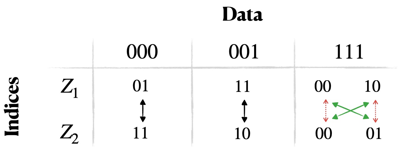
Figure 1: All possible matchings between $I({\boldsymbol{u}},Z_{1})$ and $I({\boldsymbol{u}},Z_{2})$ for every date field ${\boldsymbol{u}}\in S(z_{1}).$

The data-fields $000$ and $001$ have only one index in both $Z_{1}$ and $Z_{2}$. Thus, there is only one matching in both cases and the weight of each matching is one. On the other hand, the data-field $111$ has two indices in $Z_{1}$ and $Z_{2}$, and thus there are two optional matchings, corresponding to the dashed red one and the solid green. The weight of the red matching is 2 since $\max\{d_{H}(00,00),d_{H}(10,01)\}=2$ and the weight of the green matching is 1 since $\max\{d_{H}(00,01),d_{H}(10,00)\}=1$. Hence, $\mathcal{D}(Z_{1},Z_{2})=1$.

As will be seen later, the DNA-distance $\mathcal{D}$ will be essential in order to determine if a code is a DNA-correcting code. First, we show that $\mathcal{D}$ is a metric but not a graphic metric. Both proofs are presented in Appendix A.

Lemma 1.

The DNA-distance $\mathcal{D}$ is a metric on ${\mathcal{X}}_{M,L,\ell}$.

Claim 2.

The metric $\mathcal{D}$ is not a graphic metric.

Even though the DNA-distance is not a graphic metric, it still satisfies several properties that hold trivially for such ones. In particular, using the metric $\mathcal{D}$ it is possible to derive necessary and sufficient conditions for a code to be a DNA-correcting code, which are shown in the next subsection.

III-B Necessary and Sufficient Conditions for DNA-Correcting Codes

For a code $\mathcal{C}\subseteq{\mathcal{X}}_{M,L,\ell}$, the DNA-distance of $\mathcal{C}$ is defined by $\mathcal{D}(\mathcal{C})\triangleq\min\limits_{Z_{1}\neq Z_{2}\in\mathcal{C}}\mathcal{D}(Z_{1},Z_{2})$. Next, we draw connections between DNA-correcting codes and their DNA-distance. These connections will depend upon the value of $\tau$. First, the case $\tau=1$ is considered. In the proof of Theorem 2, we use Hall’s marriage theorem, which is stated next.

Theorem 1 (Hall, 1935).

For a finite bipartite graph $G=(L\cup R,E)$, there is an $L$-perfect matching if and only if for every subset $Y\subseteq L$ it holds that $|Y|\leq|N_{G}(Y)|$, where $N_{G}(Y)$ is the set of all vertices that are adjacent to at least one element of $Y$.

Theorem 2.

A code $\mathcal{C}\subseteq{\mathcal{X}}_{M,L,\ell}$ is a $(1,e_{i},0)_{K}$-DNA-correcting code if and only if $\mathcal{D}(\mathcal{C})>2e_{i}$.

Proof:

From Claim 1 it is sufficient to show that the claim holds for every $\mathcal{C}_{U}\subseteq\mathcal{C}$. Let $U=\{\{{\boldsymbol{u}}_{1},{\boldsymbol{u}}_{2},\dots,{\boldsymbol{u}}_{M}\}\}\in MS(\mathcal{X}_{M,L,\ell})$ and assume that $\mathcal{C}_{U}\subseteq{\mathcal{X}}_{M,L,\ell}$ is a $(1,e_{i},0)$-DNA-correcting code. Assume to the contrary that there are two codewords $Z_{1},Z_{2}\in\mathcal{C}_{U}$ such that $\mathcal{D}(Z_{1},Z_{2})\leq 2e_{i}$. It will be shown that there exists $W\in B^{K}_{1,e_{i},0}(Z_{1})\cap B^{K}_{1,e_{i},0}(Z_{2})$. For every data-field ${{\boldsymbol{u}}_{i}\in S(Z_{1})}\hskip 0.17218pt$, there exists $\pi_{i}\in BI\left((I({\boldsymbol{u}}_{i},Z_{1}),I({\boldsymbol{u}}_{i},Z_{2}))\right)$ such that $w_{H}(\pi_{i})\leq 2e_{i}$. Thus, for every index $i_{j}\in I({\boldsymbol{u}}_{i},Z_{1})$ there exists $r_{i_{j}}\in{\{0,1\}}^{\ell}$ with $d_{H}(i_{j},r_{i_{j}})\leq e_{i}$ and $d_{H}(\pi_{i}(i_{j}),r_{i_{j}})\leq e_{i}$ (since the Hamming metric is graphic). The word $W$ is built in the following way. For every index $i_{j}$ there are $K$ copies of the form $(r_{i_{j}},{\boldsymbol{u}}_{i})$, i.e., we move all the copies of each strand in both codewords to a word in the middle. It is easy to verify that $W\in B^{K}_{1,e_{i},0}(Z_{1})\cap B^{K}_{1,e_{i},0}(Z_{2})$, which is a contradiction since $\mathcal{C}$ is a $(1,e_{i},0)_{K}$-DNA-correcting code.

For the opposite direction, let $Z_{1},Z_{2}\in\mathcal{C}_{U}$ be such that $Z_{1}\neq Z_{2}$. We need to show that $B^{K}_{(1,e_{i},0)}(Z_{1})\cap B^{K}_{(1,e_{i},0)}(Z_{2})=\emptyset$. From the assumption that $\mathcal{D}(Z_{1},Z_{2})>2e_{i}$ and the definition of $\mathcal{D}$, we have that there exists a data-field ${\boldsymbol{u}}\in S(Z_{1})$ such that there is no $\pi\in BI\left((I({\boldsymbol{u}},Z_{1}),I({\boldsymbol{u}},Z_{2}))\right)$ with $w_{H}(\pi_{i})\leq 2e_{i}$. Equivalently, if we construct a bipartite graph $G=(L\cup R,E)$ where $L=I({\boldsymbol{u}},Z_{1}),R=I({\boldsymbol{u}},Z_{2})$ and $E=\{(i,j)|i\in L,j\in R,d_{H}(i,j)\leq 2e_{i}\}$ then from Hall’s marriage theorem there is a subset $Y\subseteq L$ such that $|Y|>|N_{G}(Y)|$.

We say that a read $s=(ind,{\boldsymbol{u}})$ is in the $e_{i}$ area of $Y$ if its index-field is at distance at most $e_{i}$ from at least one of the indices in $Y$. Consider a general output word $w_{1}\in B^{K}_{(1,e_{i},0)}(Z_{1})$, the number of reads in $w_{1}$ that are in the $e_{i}$ area of $Y$ is at-least $K\cdot|Y|$. On the other hand, for every $w_{2}\in B^{K}_{(1,e_{i},0)}(Z_{2})$, the number of reads in $w_{2}$ that are in the $e_{i}$ area of $Y$ is at most $K\cdot|N_{G}(Y)|<K\cdot|Y|$. Thus $B^{K}_{(1,e_{i},0)}(Z_{1})\cap B^{K}_{(1,e_{i},0)}(Z_{2})=\emptyset$. ∎

Next, we study the case of $\tau<1$ such that $\frac{K}{2}\leq\lfloor{\tau K}\rfloor$ and present a similar necessary condition for this case. The proof is similar to the first part in the proof of Theorem 2 and appears in Appendix A.

Lemma 2.

For $\tau<1$ such that $\frac{K}{2}\leq\lfloor{\tau K}\rfloor$ and $U\in MS({\mathcal{X}}_{M,L,\ell})$, if $\mathcal{C}_{U}$ is a $(\tau,e_{i},0)_{K}$-DNA-correcting code then $\mathcal{D}(\mathcal{C}_{U})>e_{i}$.

The opposite direction of Lemma 2 does not hold in general, however, it holds if one assures that all data-fields in the stored sets are different. Let $\overline{\mathcal{X}}_{M,L,\ell}$ denote all such sets, i.e., ${\overline{\mathcal{X}}_{M,L,\ell}=\{Z\in\mathcal{X}_{M,L,\ell}|\ |S(Z)|=M\}}.$ Note that the size of $\overline{\mathcal{X}}_{M,L,\ell}$ is ${2^{\ell}\choose M}{2^{L-\ell}\choose M}M!$, and that $\overline{\mathcal{X}}_{M,L,\ell}\neq\emptyset$ if and only if $L-\ell\geq\log_{2}(M)$. Although restricting to only sets in $\overline{\mathcal{X}}_{M,L,\ell}$ might reduce the number of information bits that is possible to store in the DNA storage system, it is verified in the next lemma, using the results from [16], that for practical values of $\beta$ there is only a single-bit reduction. The proof appears in Appendix A.

Lemma 3.

For $\beta<\frac{1}{2}\left(1-\frac{\ell}{L}\right)$ it holds that $r(\overline{\mathcal{X}}_{M,L,\ell})<1.$ Furthermore, for $\beta\leq\frac{\ln(2)(L-\ell)+2\ell}{L(\ln(2)+2\ell)}$ there exists an efficient construction of $\overline{\mathcal{X}}_{M,L,\ell}$ that uses a single redundancy bit.

The notation $MS(\overline{\mathcal{X}}_{M,L,\ell})$ is used to denote the set of all possible data-field multisets of elements in $\overline{\mathcal{X}}_{M,L,\ell}$, which are in essence sets. The next lemma presents a sufficient condition for such sets, the proof is similar to the proof of the sufficient condition of Theorem 2 and presented in Appendix A.

Lemma 4.

For $\tau<1$ such that $\frac{K}{2}\leq\lfloor{\tau K}\rfloor$ and $U\in MS(\overline{\mathcal{X}}_{M,L,\ell})$, if $\mathcal{D}(\mathcal{C}_{U})>e_{i}$ then $\mathcal{C}_{U}$ is a $(\tau,e_{i},0)_{K}$-DNA-correcting code.

The next corollary summarizes this discussion.

Corollary 2.

For $\tau<1$ such that $\frac{K}{2}\leq\lfloor{\tau K}\rfloor$ and $U\in MS(\overline{\mathcal{X}}_{M,L,\ell})$, $\mathcal{C}_{U}$ is a $(\tau,e_{i},0)_{K}$-DNA-correcting code if and only if $\mathcal{D}(\mathcal{C}_{U})>e_{i}$.

We continue to study the case of $\tau$ such that $\lfloor{\tau K}\rfloor<\frac{K}{2}$ in the next two lemmas, while both proofs are presented in Appendix A.

Lemma 5.

For $\tau$ such that $\lfloor{\tau K}\rfloor<\frac{K}{2}$, it holds that for every $e_{i}$, $\overline{\mathcal{X}}_{M,L,\ell}$ is a $(\tau,e_{i},0)_{K}$-DNA-correcting code.

Lemma 6.

For $\tau$ such that $\lfloor{\tau K}\rfloor<\frac{K}{2}$, if $\mathcal{C}\subseteq\mathcal{X}_{M,L,\ell}$ is a code with $\mathcal{D}(\mathcal{C})>e_{i}$ then $\mathcal{C}$ is a $(\tau,e_{i},0)_{K}$-DNA-correcting code.

III-C Codes for a Fixed Data-Field Set

So far in the paper we focused on properties and conditions of DNA-correcting codes that guarantee successful decoding of the data. In particular, Corollary 1 showed that it is enough to construct codes for every data-field multiset $U\in MS({\mathcal{X}}_{M,L,\ell})$ independently, while the conditions with respect to the DNA-distance were established in Theorem 2, and Lemmas 2, 4, 5 and 6. These conditions depend upon the value of $\tau$ and whether $U$ is a set/multiset. In Lemma 3, it was shown that for all practical values of $\beta$, restricting to using only sets in $\overline{\mathcal{X}}_{M,L,\ell}$ imposes only a single bit of redundancy and therefore, the rest of the paper provides DNA-correcting codes for $\overline{\mathcal{X}}_{M,L,\ell}$.

Note that for $U,U^{\prime}\in MS(\overline{\mathcal{X}}_{M,L,\ell})$ it holds that $A_{M,L,\ell}(\tau,e_{i},0,K)_{U}=A_{M,L,\ell}(\tau,e_{i},0,K)_{U^{\prime}}$ and thus for the rest of the paper we fix $U=\{{\boldsymbol{u}}_{1},{\boldsymbol{u}}_{2},\dots,{\boldsymbol{u}}_{M}\}\in MS(\overline{\mathcal{X}}_{M,L,\ell})$ and our goal is to find DNA-correcting codes for $U$ with a given DNA-distance. Note that for $Z=\{(ind_{1},{\boldsymbol{u}}_{1}),\dots,(ind_{M},{\boldsymbol{u}}_{M})\},Z^{\prime}=\{(ind_{1}^{\prime},{\boldsymbol{u}}_{1}),\dots,(ind_{M}^{\prime},{\boldsymbol{u}}_{M})\}$, it holds that

$$\mathcal{D}(Z_{1},Z_{2})=\max_{1\leq i\leq M}d_{H}(ind_{i},ind_{i}^{\prime}).$$

Thus, we focus on studying the next family of codes for the index-fields.

Definition 2.

Let $I(\ell,M)=\{(ind_{1},\dots,ind_{M})|\forall i:ind_{i}\in\{{0,1}\}^{\ell},\forall i\neq j:ind_{i}\neq ind_{j}\}$. For every two codewords ${\boldsymbol{c}}=(c_{1},\ldots,c_{M}),{\boldsymbol{c}}^{\prime}=(c^{\prime}_{1},\ldots,c^{\prime}_{M})\in I(\ell,M)$, their index-distance is defined by $\mathcal{D}_{I}({\boldsymbol{c}},{\boldsymbol{c}}^{\prime})\triangleq\max\limits_{1\leq i\leq M}d_{H}(c_{i},c_{i}^{\prime})$ and for a code $\mathcal{C}\subseteq I(\ell,M)$, its index-distance is defined by $\mathcal{D}_{I}(\mathcal{C})\triangleq\min\limits_{{\boldsymbol{c}}\neq{\boldsymbol{c}}^{\prime}\in\mathcal{C}}\mathcal{D}_{I}({\boldsymbol{c}},{\boldsymbol{c}}^{\prime})$. A code $\mathcal{C}\subseteq I(\ell,M)$ will be called an $(\ell,M,d)$ index-correcting code if $\mathcal{D}_{I}(\mathcal{C})\geq d$. We denote by $F(\ell,M,d)$ the size of a maximal $(\ell,M,d)$ index-correcting code.

Example 2.

The rows of the following matrix form a $(2,4,2)$ index-correcting code, while each row corresponds to a codeword,

$$P=\begin{pmatrix}00&01&11&10\\ 00&11&10&01\\ 00&10&01&11\\ 11&01&00&10\\ 11&00&10&01\\ 11&10&01&00\end{pmatrix}.$$ (2)

One can verify, that for every two different rows $i,i^{\prime}$, there exists a column $j$ such that $d_{H}(P(i,j),P(i^{\prime},j))=2$.

The motivation for studying this family of codes comes from the following observation which results from Theorem 2, Corollary 2, and Lemma 5.

Observation 1.

For $U\in MS(\overline{\mathcal{X}}_{M,L,\ell})$, it holds that

$$A_{M,L,\ell}(\tau,e_{i},0,K)_{U}=\begin{cases}F(\ell,M,2e_{i}+1),&\tau=1\\ F(\ell,M,e_{i}+1),&\frac{K}{2}\leq\lfloor{\tau K}\rfloor<K\\ {2^{\ell}\choose M}M!,&\lfloor{\tau K}\rfloor<\frac{K}{2}\end{cases}$$

Note that the study of index-correcting codes and in particular the value of $F(\ell,M,d)$ is interesting on its own and can be useful for other problems, independently of the problem of designing codes for DNA storage. The next section is dedicated to a careful investigation of these codes.

IV Index-Correcting Codes

We start by studying the special case of $\ell=\log(M)$.

IV-A $\ell=\log(M)$

In this case, every possible codeword in $I(\log(M),M)$ is a permutation over $\{0,1\}^{\log(M)}$, and for $f,g\in I(\log(M),M)$, their DNA-distance is equivalent to the $\ell_{\infty}$ distance over the Hamming distance of the indices, i.e., $\mathcal{D}_{I}(f,g)=\max\limits_{i\in\{0,1\}^{\log(M)}}d_{H}(f(i),g(i))$. For $f\in I(\log(M),M)$, let $B_{r}(f)$ be the ball of radius $r$ centered at $f$ in $I(\log(M),M)$, i.e.,

$$B_{r}(f)=\{g\in I(\log(M),M)|\mathcal{D}_{I}(f,g)\leq r\}.$$

In this case, it holds that $\mathcal{D}_{I}$ is right invariant, i.e., for $f,g,p\in I(\log(M),M)$ it holds that $\mathcal{D}_{I}(f,g)=\mathcal{D}_{I}(f\circ p,g\circ p)$, and thus the size of the balls is the same. Let $B_{r,M}$ denote the size of the balls of radius $r$ in $I(\log(M),M)$. An important matrix with respect to $B_{r,M}$ is the matrix $A_{r,M}=(a_{i,j})$ of size $M\times M$ which is defined by

$$a_{i,j}={\begin{cases}1&d_{H}(i,j)\leq r\\ 0&\text{otherwise}\end{cases}},i,j\in\{0,1\}^{\log(M)}.$$

Let $per(A)$ denote the permanent of a square matrix $A$. Then the next lemma, which follows in a similar way to the one presented in [15], holds. For completeness, the proof and the definition of a permanent of a matrix are shown in Appendix A.

Lemma 7.

It holds that $B_{r,M}=per(A_{r,M})$.

Next, two bounds on $F(\log(M),M,d)$ are presented. Lemma 8 uses the sphere packing bound with a known bound on the permanent of a matrix, while Lemma 9 uses a method that is similar to the proof of the Singleton bound.

Lemma 8.

Let $r(d,M)=\sum_{i=0}^{\lfloor\frac{d-1}{2}\rfloor}{\log(M)\choose i}$ then $F(\log(M),M,d)\leq\frac{M!}{(r(d,M)!)^{\frac{M}{r(d,M)}}}$.

Proof:

It is known that for an $n\times n$ $(0,1)$ matrix $A$ it holds that $per(A)\leq\prod_{i=1}^{n}r_{i}!^{\frac{1}{r_{i}}}$, where $r_{i}$ is the number of ones in row $i$. Note that the number of ones in every row of the matrix $A_{\lfloor\frac{d-1}{2}\rfloor,M}$ is exactly $r(d,M)$. Thus $B_{\lfloor\frac{d-1}{2}\rfloor,M}\leq(r(d,M)!)^{\frac{M}{r(d,M)}}$. The lemma follows since the balls with radius $\lfloor\frac{d-1}{2}\rfloor$ are mutually disjoint. ∎

Lemma 9.

$F(\log(M),M,d)\leq\frac{M!}{(2^{d-1}!)^{2^{\log(M)-d+1}}}$.

Proof:

Let $\mathcal{C}$ be a $(\log(M),M,d)$ index-correcting code and let $P$ be the matrix whose rows are the codewords of $\mathcal{C}$. Given a row of indices in $P$, $ind_{1},ind_{2},\ldots,ind_{M}$, we divide every such $ind_{j}$ to two parts, $a_{j}\in\{0,1\}^{\ell-d+1}$ which is the first $\ell-d+1$ bits of $ind_{j}$ and $b_{j}\in\{0,1\}^{d-1}$ which is the last $d-1$ bits of $ind_{j}$. We concatenating all $a_{j}$ to form a vector $\overline{a}\in\left(\{{0,1\}^{\ell-d+1}}\right)^{M}$. Note that every such vector $\overline{a}$ can only appear once in $P$ (as if there are two different rows $i$ $i^{\prime}$ that form this vector, then the hamming distance between indices of the same column is at most $d-1$, which implies that the $d$ distance between those two rows is at most $d-1<d$). Hence, the number of possible rows in $P$, is bounded above by the number of possible vectors $\overline{a}\in\left(\{{0,1\}^{\ell-d+1}}\right)^{M}$. Since all the $\{0,1\}^{\ell}$ indices must appear in every row, every vector in $\{0,1\}^{\ell-d+1}$ must appear $2^{d-1}$ times in $\overline{a}$. Thus, from the multinomial theorem the number of possible vectors $\overline{a}$ is $\frac{M!}{(2^{d-1}!)^{2^{log(M)-d+1}}}$. Since we started with a general $(\log(M),M,d)$ index-correcting code, we conclude that $F(\log(M),M,d)\leq\frac{M!}{(2^{d-1}!)^{2^{\log(M)-d+1}}}$. ∎

Note, that the code in Example 2 achieves the bound in Lemma 9, and hence this bound can be tight in some cases.

Next, we present a construction by building a matrix whose rows form an $(\log(M),M,d)$ index-correcting code. Such a matrix whose rows form an $(\ell,M,d)$ index-correcting code will be called an $(\ell,M,d)$-matrix. The construction uses codes over $\{0,1\}^{\log(M)}$ with Hamming distance $d$ and afterward an example for small values of $d$ is presented.

Construction 1.

Let there be an optimal, with respect to the Hamming distance, linear code $\mathcal{C}$ over $\{0,1\}^{\log(M)}$ with distance $d$. Denote by $A$ the size of $\mathcal{C}$ and note that the $\frac{M}{A}$ cosets of $\mathcal{C}$ form a partition of $\{0,1\}^{\log(M)}$. Denote the cosets of $\mathcal{C}$ by $\mathcal{C}_{1}=\mathcal{C},\mathcal{C}_{2},\dots,\mathcal{C}_{\frac{M}{A}}$. We start by building a matrix that consists of $(A!)^{\frac{M}{A}}$ rows, where the first $A$ entries of every row are permutations over the first coset, the second $A$ entries are permutations over the second coset, and so on. Since the entries of every column belong to the same coset, the distance between different rows is at least $d$. Next, we take every coset $\mathcal{C}_{i}$ for $2\leq i\leq\frac{M}{A}$ and remove from it all words that are at distance at most $d$ from the zero vector $\mathbf{0}$, and denote by $\mathcal{C}^{\prime}_{i}$ the achieved codes. Then, for every $c^{\prime}\in\mathcal{C}^{\prime}_{i}$, we can look at all the rows in the matrix where $c^{\prime}$ and $\mathbf{0}$ are fixed to the first entry of their coset (note that there are $(A-1)!^{2}(A!)^{\frac{M}{A}-2}$ such rows) and add the same row where we replace the entry of $c^{\prime}$ with $\mathbf{0}$. Since we do so for every $i$ we have $(\frac{M}{A}-1)|\mathcal{C}^{\prime}|\frac{1}{A^{2}}(A!)^{\frac{M}{A}}$ more rows.

Example 3.

We apply Construction 1 to the case of $d=2$ and $d=3$. For $d=2$ we have that the maximal linear code $\mathcal{C}$ is the parity with $|\mathcal{C}|=\frac{M}{2}$, and that $|\mathcal{C}^{\prime}|=\frac{M}{2}-\log(M)$. Thus in this case we get a $(\log(M),M,2)$ index-correcting code with size of $(\frac{M}{2}!)^{2}+(\frac{M}{2}-\log(M))(\frac{M-2}{2}!)^{2}$. For $d=3$ and $\log(M)=\ell=2^{m}-1$ we have that the maximal linear code $\mathcal{C}$ is the binary Hamming code with $|\mathcal{C}|=2^{2^{m}-1-m}$, and that there are $2^{m}$ cosets (including the code itself). In addition, every coset $\mathcal{C}_{i}\neq\mathcal{C}$ has one word of weight $1$ and $\frac{2^{m}-2}{2}$ words of weight $2$. Thus we have a $(2^{m}-1,2^{2^{m}-1},3)$ index-correcting code with size of $(\frac{M}{\log(M)+1}!)^{\log(M)+1}\left(1+g(M)\right)$, where $g(M)=\Theta(\frac{\log^{2}(M)}{M})$. For more detailed analyses, see Appendix A.

IV-B $\ell>\log(M)$

In this case, the set of possible indices is larger than the number of strands. We show how to construct an $(\ell^{\prime},M,d)$ index-correcting code from an $(\ell,M,d)$ index-correcting code for $\ell<\ell^{\prime}$.

Lemma 10.

For $\ell^{\prime}=\ell+\lceil\frac{d}{2}\rceil$ it holds that $F(\ell^{\prime},M,d)\geq F(\ell,M,d)\times 2^{M}$

Proof:

We show a construction of a matrix $P^{\prime}$ using a maximal $(\ell,M,d)$-matrix  $P$ with $F(\ell,M,d)$ rows and the proof that the matrix $P^{\prime}$ is a legal $(\ell^{\prime},M,d)$-matrix with $F(\ell,M,t)\times 2^{M}$ rows appears in Appendix A. The construction is specified next iteratively.

1. Obtain a matrix $P^{\prime}_{0}$ by adding $\lceil\frac{d}{2}\rceil$ bits of $0$ at the end of every entry in $P$.

2. For $j=1,2,\ldots,M$: For every row $i$ of $P^{\prime}_{j-1}$, add a similar row $b_{j}(i)$ which differs from the $i$-th row only in the $j$-th column. The difference is that in $b_{j}(i)$, the first and last $\lceil\frac{d}{2}\rceil$ bits of the $j$-th entry, are the transpose of the corresponding entry in row $i$. We denote the matrix obtained after the $j^{\prime}th$ step by $P^{\prime}_{j}$.

We left to show that the above construction ends with a legal $(\ell^{\prime},M,d)$-matrix with $F(\ell,M,t)\times 2^{M}$ rows. First, since for every $j$ the number of rows is multiplied by two, we have in the end a matrix $P^{\prime}=P^{\prime}_{M}$ with $F(\ell,M,t)\times 2^{M}$ rows.

Next, we show by induction that after every step $j$, $P^{\prime}_{j}$ is a $(\ell^{\prime},M,d)$-matrix. The base case is simple, as $P$ is a $(\ell,M,d)$-matrix and hence $P^{\prime}_{0}$ is a $(\ell^{\prime},M,d)$-matrix. For the induction step, on step $j$ we start with a matrix $P^{\prime}_{j-1}$ which is a $(\ell^{\prime},M,d)$-matrix. First, note, that the indices in every row in $P^{\prime}_{j}$ are disjoint, since otherwise we can apply the inverse of transposing the last and first $\lceil\frac{d}{2}\rceil$ of these indices and have that there was a row in $P^{\prime}_{0}$ which had two identical indices. Now, take two general rows $i,i^{\prime}\in P^{\prime}_{j-1}$, the distance for rows $b_{j}(i),b_{j}(i^{\prime})$ is the same as the distance of rows $i,i^{\prime}$, and the distance between rows $i$ and $b_{j}(i)$ is $\lceil\frac{d}{2}\rceil+\lceil\frac{d}{2}\rceil\geq d$ (as they differ in the first and last $\lceil\frac{d}{2}\rceil$ components in index $j$). Thus, we left to check the distance condition for rows $i$ and $b_{j}(i^{\prime})$. But the distance between rows $i,b_{j}(i^{\prime})$ can only increase from the distance between rows $i,i^{\prime}$ and $P_{j}^{\prime}(i)$ is a $(\ell^{\prime},M,d)$-matrix, thus the distance property holds and $P^{\prime}_{j}$ is a $(\ell^{\prime},M,d)$-matrix. ∎

Example 4.

The next matrix is the matrix obtained from the matrix in Example 2 after step $j=1$.

$$P^{\prime}_{1}=\begin{pmatrix}000&010&110&100\\ 000&110&100&010\\ 000&100&010&110\\ 110&010&000&100\\ 110&000&100&010\\ 110&100&010&000\\ 101&010&110&100\\ 101&110&100&010\\ 101&100&010&110\\ 011&010&000&100\\ 011&000&100&010\\ 011&100&010&000\end{pmatrix}$$ (3)

V Generalizations and Future Work

Note, that in all the proof of the necessary and sufficient conditions, only the fact that the Hamming metric is graphic was used. Thus all the results for $e_{d}=0$ hold also when replacing every instance of the Hamming distance with the edit distance. The case of $e_{d}>0$ is more complicated since Claim 1 does not hold for $e_{d}>0$. Nonetheless, if one wishes to construct a $(\tau,e_{i},e_{d})_{K}$-DNA-correcting code  $\mathcal{C}_{U}$ for $U\in MS(\mathcal{X}_{M,L,\ell})$ with DNA distance larger than $2e_{d}+1$, then the constructions in Section IV will work. For future work, we plan to continue studying the value of $F(\ell,M,d)$, especially for $\ell>\log(M)$ which is an interesting and important question, as well as to study the case of $e_{d}>0$, and in particular, find necessary and sufficient conditions for this case.

VI Acknowledgments

We would like to thank Prof. Tuvi Etzion for helping us analyze the DNA-Distance and Prof. Moshe Schwartz for helping us in studying the $\ell_{\infty}$ distance over the Hamming distance of the indices.

Appendix A

See 1

Proof:

Let $Z_{1},Z_{2},Z_{3}\in{\mathcal{X}}_{M,L,\ell}$. In order to show that $\mathcal{D}$ is indeed a metric, let us prove the three properties of a metric:

1. $\mathcal{D}(Z_{1},Z_{2})=0\text{ if and only if }Z_{1}=Z_{2}$.

   If $Z_{1}=Z_{2}$ then for every data-field ${\boldsymbol{u}}$ we consider the trivial matching that sends every index to itself, hence $\mathcal{D}(Z_{1},Z_{2})=0$. For the other direction, if $\mathcal{D}(Z_{1},Z_{2})=0$ then both words have the same data-field multiset, and in the minimal matching for every data-filed, every index is matched to itself (otherwise the distance would be greater than $0$), thus the indices for every data-field ${\boldsymbol{u}}$ are the same in both sets and hence $Z_{1}=Z_{2}$.

2. $\mathcal{D}(Z_{1},Z_{2})=\mathcal{D}(Z_{2},Z_{1})$.

   Since there is no difference between matching the indices in $Z_{1}$ and the indices in $Z_{2}$ or vice versa, the definition of the distance is symmetric.

3. $\mathcal{D}(Z_{1},Z_{3})\leq\mathcal{D}(Z_{1},Z_{2})+\mathcal{D}(Z_{2},Z_{3})$.

   If $Z_{1}\text{ and }Z_{3}$ do not have the same data-field multiset then at least $Z_{1}\text{ and }Z_{3}$ or $Z_{2}\text{ and }Z_{3}$ have different data-field multiset, and the right-hand side will be equal to $\infty$ as well. Assume that $Z_{1},Z_{2},Z_{3}$ have the same data-field multiset $\{\{{\boldsymbol{u}}_{1},{\boldsymbol{u}}_{2},\dots,{\boldsymbol{u}}_{M}\}\}$. Let $\pi_{i,j}$ denote the matching between the indices of $Z_{i}$ and $Z_{j}$, where every index of data-field ${\boldsymbol{u}}$ is matched according to the minimal Hamming weight matching in $BI(I{({\boldsymbol{u}},Z_{i})},I{({\boldsymbol{u}},Z_{j})})$. We show that for every ${\boldsymbol{u}}$ the triangle inequality holds and our claim will follow. Let there be ${\boldsymbol{u}}\in S(Z_{1})$ and let $\mathcal{D}(Z_{1},Z_{2})_{\boldsymbol{u}}$ be the distance when focusing on the data-field ${\boldsymbol{u}}$. Then, it holds that

   $$\mathcal{D}(Z_{1},Z_{2})_{\boldsymbol{u}}+\mathcal{D}(Z_{2},Z_{3})_{\boldsymbol{u}}=\max\limits_{i\in I({\boldsymbol{u}},Z_{1})}d_{H}(i,\pi_{1,2}(i))$$

   $$+\max\limits_{i\in I({\boldsymbol{u}},Z_{1})}d_{H}\left(\pi_{1,2}(i),\pi_{2,3}(\pi_{1,2}(i))\right)$$

   $$\geq\max\limits_{i\in I({\boldsymbol{u}},Z_{1})}\{d_{H}(i,\pi_{1,2}(i))+d_{H}\left(\pi_{1,2}(i),\pi_{2,3}(\pi_{1,2}(i))\right)\}$$

   $$\overset{\mathrm{(a)}}{\geq}\max\limits_{i\in I({\boldsymbol{u}},Z_{1})}\{d_{H}(i,\pi_{23}(\pi_{12}(i))\}\overset{\mathrm{(b)}}{\geq}\mathcal{D}(Z_{1},Z_{3})_{\boldsymbol{u}}.$$

   where (a) holds since the Hamming distance is a metric and (b) is true because $\pi_{23}\circ\pi_{12}\in BI(I({\boldsymbol{u}},Z_{1}),I({\boldsymbol{u}},Z_{3}))$.

∎

See 2

Proof:

Let there be the following two sets in $\mathcal{X}_{4,L,4}$

$$Z_{1}=\{(0000,{\boldsymbol{u}}_{1}),(1100,{\boldsymbol{u}}_{2}),(1010,{\boldsymbol{u}}_{3}),(1001,{\boldsymbol{u}}_{4})\},$$

$$Z_{2}=\{(0000,{\boldsymbol{u}}_{2}),(1100,{\boldsymbol{u}}_{1}),(1010,{\boldsymbol{u}}_{4}),(1001,{\boldsymbol{u}}_{3})\},$$

where all the data-fields are different. On one hand, since for every data-field, the Hamming distance between the corresponding indices is 2 it holds that $\mathcal{D}(Z_{1},Z_{2})=2$. On the other hand, if the metric was graphic, the shortest path between $Z_{1}$ and $Z_{2}$ in the corresponding graph would be 2 as well, which implies that there would be a word $Z\in\mathcal{X}_{4,L,4}$ such that $Z\in B_{1}(Z_{1})\cap B_{1}(Z_{2})$. But for it to happen, $Z$ must have the same data-field multiset as $Z_{1}$ and $Z_{2}$, and the indices of ${\boldsymbol{u}}_{1}$ and ${\boldsymbol{u}}_{2}$ must be $\{1000,0100\}$, and the indices of ${\boldsymbol{u}}_{3}$ and ${\boldsymbol{u}}_{4}$ must be $\{1000,1011\}$. We get three indices for four data parts, and hence $B_{1}(Z_{1})\cap B_{1}(Z_{2})=\emptyset$. ∎

See 2

Proof:

Similar to the proof of the necessary condition in Theorem 2, let $U=\{\{{\boldsymbol{u}}_{1},{\boldsymbol{u}}_{2},\dots,{\boldsymbol{u}}_{M}\}\}\in MS(\mathcal{X}_{M,L,\ell})$ and assume that $\mathcal{C}_{U}\subseteq{\mathcal{X}}_{M,L,\ell}$ is a $(\tau,e_{i},0)$-DNA-correcting code. Assume to the contrary that there are two codewords $Z_{1},Z_{2}\in\mathcal{C}_{U}$ such that $\mathcal{D}(Z_{1},Z_{2})\leq e_{i}$. It will be shown that there exists $W\in B^{K}_{\tau,e_{i},0}(Z_{1})\cap B^{K}_{\tau,e_{i},0}(Z_{2})$. For every data-field ${{\boldsymbol{u}}_{i}\in S(Z_{1})}\hskip 0.17218pt$, there exists $\pi_{i}\in BI\left((I({\boldsymbol{u}}_{i},Z_{1}),I({\boldsymbol{u}}_{i},Z_{2}))\right)$ such that $w_{H}(\pi_{i})\leq e_{i}$. Thus, for every index $i_{j}\in I({\boldsymbol{u}}_{i},Z_{1})$ there exists a matched index $\pi_{i}(i_{j})\in I({\boldsymbol{u}}_{i},Z_{2})$ with $d_{H}(i_{j},\pi_{i}(i_{j}))\leq e_{i}$. The word $W$ is built in the following way. For every index $i_{j}$ there are $\lfloor\frac{K}{2}\rfloor$ copies of the from $({i_{j}},{\boldsymbol{u}}_{i})$ and $\lceil\frac{K}{2}\rceil$ copies of the from $(\pi_{i}({i_{j}}),{\boldsymbol{u}}_{i})$, i.e., we move $\lceil\frac{K}{2}\rceil$ copies of each strand in $Z_{1}$ to its matched strand index in $Z_{2}$. Since $\frac{K}{2}\leq\lfloor\tau K\rfloor$ it holds that $\lceil\frac{K}{2}\rceil\leq\lfloor\tau K\rfloor$ and hence $W\in B^{K}_{\tau,e_{i},0}(Z_{1})$. In addition $W$ can be obtained by taking every strand in $Z_{2}$ of the form $(\pi_{i}({i_{j}}),{\boldsymbol{u}}_{i})$ and move $\lfloor\frac{K}{2}\rfloor$ copies to $({i_{j}},{\boldsymbol{u}}_{i})$. Hence $W\in B^{K}_{\tau,e_{i},0}(Z_{1})\cap B^{K}_{\tau,e_{i},0}(Z_{2})$, which is a contradiction since $\mathcal{C}$ is a $(\tau,e_{i},0)_{K}$-DNA-correcting code ∎

See 3

Proof:

Denote $L^{\prime}=L-\ell$, we have that

$$r(\overline{\mathcal{X}}_{M,L,\ell})=\log(|{\mathcal{X}}_{M,L,\ell}|)-\log(|\overline{\mathcal{X}}_{M,L,\ell}|)$$

$$=\log\left({2^{\ell}\choose M}{2^{(L-\ell)M}}\right)-\log\left({2^{\ell}\choose M}{2^{L-\ell}\choose M}M!\right)$$

$$=\log(2^{(L-\ell)M})-\log({2^{L-\ell}\choose M}M!)$$

$$=\log(2^{L^{\prime}M})-\log(\frac{2^{L^{\prime}}!}{(2^{L^{\prime}}-M)!})$$

$$=\log(\frac{2^{L^{\prime}}\cdot 2^{L^{\prime}}\cdots 2^{L^{\prime}}}{2^{L^{\prime}}(2^{L^{\prime}}-1)\cdots(2^{L^{\prime}}-M+1)})=$$

$$\log(\prod_{i=0}^{M-1}\frac{2^{L^{\prime}}}{2^{L^{\prime}}-i})=-\log(\prod_{i=0}^{M-1}(1-\frac{i}{2^{L^{\prime}}})$$

Using the inequality $(1-a)(1-b)>1-(a+b)$ for $a,b>0$, we get that $\prod_{i=0}^{M-1}(1-\frac{i}{2^{L^{\prime}}})>1-\sum_{i=0}^{M-1}\frac{i}{2^{L^{\prime}}}=1-\frac{M(M-1)}{2^{L^{\prime}+1}}>1-\frac{M^{2}}{2^{L^{\prime}+1}}$. Thus, since $-\log$ is a monotonic decreasing function, it is derived that

$$r(\overline{\mathcal{X}}_{M,L,\ell})<-\log(1-\frac{M^{2}}{2^{L^{\prime}+1}}).$$

Lastly, since $\beta<\frac{1}{2}\left(1-\frac{\ell}{L}\right)$ we have that $\frac{M^{2}}{2^{L^{\prime}+1}}=\frac{2^{2\beta L}}{2^{L-\ell+1}}=2^{L(2\beta-1)+\ell-1}<\frac{1}{2}$. Thus, we conclude that $r(\overline{\mathcal{X}}_{M,L,\ell})<-\log(1-\frac{M^{2}}{2^{L^{\prime}+1}})<-\log(1-\frac{1}{2})=1$.

Regarding the construction, in [16], the authors present such a construction in the case that

$$1\leq\frac{L-\ell-\log(M)-\ell\log\log(M)+\log(L-\ell)}{\log(L-\ell)+\ell\log\log(M)}$$

.

This happens if and only if $2\ell\log(\beta L)\leq L-\ell-\beta L.$ Using the inequality that $\ln(x)<x-1$ for $x>0$ we have that $2\ell\log(\beta L)\leq\frac{2\ell}{\ln(2)}(\beta L-1)$. Thus if the following inequality holds $\frac{2\ell}{\ln(2)}(\beta L-1)\leq L-\ell-\beta L$, we get the desired quality. And this holds if and only if $\beta\leq\frac{\ln(2)(L-\ell)+2\ell}{L(\ln(2)+2\ell)}.$ ∎

See 4

Proof:

The proof is similar to the proof of the sufficient condition in Theorem 2. Let $Z_{1},Z_{2}\in\mathcal{C}_{U}$ be such that $Z_{1}\neq Z_{2}$. We need to show that $B^{K}_{(\tau,e_{i},0)}(Z_{1})\cap B^{K}_{(\tau,e_{i},0)}(Z_{2})=\emptyset$. From the assumption that $\mathcal{D}(Z_{1},Z_{2})>e_{i}$ and the definition of $\mathcal{D}$, we have that there exists a data-field ${\boldsymbol{u}}\in S(Z_{1})$ such that $d_{H}(I({\boldsymbol{u}},Z_{1}),I({\boldsymbol{u}},Z_{2}))\geq e_{i}$. Since $\tau<1$ in every general output $w_{1}\in B^{K}_{(\tau,e_{i},0)}(Z_{1})$ there will be at least one read of the form $(I({\boldsymbol{u}},Z_{1}),{\boldsymbol{u}})$, on the other hand since $d_{H}(I({\boldsymbol{u}},Z_{1}),I({\boldsymbol{u}},Z_{2}))\geq e_{i}$ in every general output $w_{2}\in B^{K}_{(\tau,e_{i},0)}(Z_{2})$ there will $0$ reads of the form $(I({\boldsymbol{u}},Z_{1}),{\boldsymbol{u}})$. Hence, $B^{K}_{(\tau,e_{i},0)}(Z_{1})\cap B^{K}_{(\tau,e_{i},0)}(Z_{2})=\emptyset$. ∎

See 5

Proof:

In this case, the output strands enjoy from the property which is referred at [16] as the dominance property, i.e, if the strands clustered by their index, and every such cluster is partitioned into subsets based on the original index part, the largest subset will be the correct subset. This is indeed the situation, as the data part of every strand is different and free of errors, thus, the correct subset would be of size at least $\lfloor\frac{K}{2}\rfloor+1$ while all others subsets would be of size at most $\lfloor\frac{K}{2}\rfloor$. Hence the naive algorithm which clusters the strands by their index and matches every index with the data that fits with the largest subset of this cluster, retrieves the original input successfully. ∎

See 6

Proof:

The proof is similar to the sufficient condition of Theorem 2 and thus we describe only the differences. The first difference is that when building the graph for the indices of $Z_{1}$ and $Z_{2}$ of the problematic data-field ${\boldsymbol{u}}$, the edges connect indices with distance at most $e_{i}$, then as in Theorem 2, there is $Y\subseteq L$ such that $|Y|>|N_{G}(Y)|$. The final claim is that for every general output $w_{1}\in B^{K}_{(\tau,e_{i},0)}(Z_{1})$, the number of reads in $w_{1}$ that are in the $0$ area of $Y$ (meaning the read didn’t suffer from errors) is at-least $\frac{1}{2}K\cdot|Y|$ (because $\lfloor{\tau K}\rfloor<\frac{K}{2}$). On the other hand, for every $w_{2}\in B^{K}_{(\tau,e_{i},0)}(Z_{2})$, the number of reads in $w_{2}$ that are in the $0$ area of $Y$ is at most $\frac{1}{2}K\cdot|N_{G}(Y)|<\frac{1}{2}K\cdot|Y|$. Thus $B^{K}_{(\tau,e_{i},0)}(Z_{1})\cap B^{K}_{(\tau,e_{i},0)}(Z_{2})=\emptyset$.

∎

Definition 3.

Let $S_{n}$ denote all permutations over $[n]$. For an $n\times n$ matrix $A=(a_{i,j})$, the permanent of $A$ is defined as $per(A)\triangleq\sum\limits_{f\in S_{n}}\prod\limits_{i\in[n]}a_{i,f(i)}$.

See 7

Proof:

Let $ID_{M}$ be the trivial permutation over $\{0,1\}^{\log(M)}$. Then $B_{r,M}=B_{r,M}(ID_{M})$ and from the definition of a permanent we have that:

$$per(A_{r,M})=\sum_{f\in S_{M}}\prod_{i\in\{0,1\}^{\log(M)}}a_{i,f(i)}$$

$$\overset{\mathrm{(a)}}{=}|\{f\in S_{M})|\forall i\in\{0,1\}^{\log(M)}:d_{H}(i,f(i))\leq r\}|$$

$$=|\{f\in S_{M})|\mathcal{D}_{I}(ID_{M},f)\leq r\}|=|B_{r,M}(ID_{M})|$$

$$=B_{r,M}$$

Where (a) holds because of the shape of the matrix $A_{r,M}$. ∎

Example 3. Here we extend the analyses for Example 3. In the case of $d=3$ and $\log(M)=\ell=2^{m}-1$. In this case we have that $|\mathcal{C}|=2^{2^{m}-1-m}$ and that there are $2^{m}$ cosets, where every coset $\mathcal{C}_{i}\neq\mathcal{C}$ has one word of weight $1$ and $\frac{2^{m}-2}{2}$ words of weight $2$, thus $|\mathcal{C}^{\prime}_{i}|=2^{2^{m}-1-m}-\frac{2^{m}-4}{2}$. Hence, applying Construction 1 we get an $(2^{m}-1,2^{2^{m}-1},3)$ index-correcting code with size of $(2^{2^{m}-1-m}!)^{2^{m}}(1+(2^{m}-1)|\mathcal{C}^{\prime}_{i}|\frac{1}{(2^{2^{m}-1-m})^{2}})=*$

Using that $m=\log(\ell+1)=\log(\log(M)+1)$ we have that

$$*=(\frac{M}{\log(M)+1}!)^{\log(M)+1}(1+\log(M)$$

$$(\frac{2M-\log^{2}(M)+2\log(M)+3}{2\log(M)+2})(\frac{(\log(M)+1)^{2}}{M^{2}}))=$$

$$(\frac{M}{\log(M)+1}!)^{\log(M)+1}(1+\Theta(\frac{\log^{2}(M)}{M})).$$

References

- [1] L. Anavy, I. Vaknin, O.Atar, R. Amit and Z. Yakhini, "Data storage in DNA with fewer synthesis cycles using composite DNA letters". Nat. Biotechnol. 37, 2019.
- [2] D. Bar-Lev, I. Orr, O. Sabary, T. Etzion, and E. Yaakobi, “Deep DNA storage: Scalable and robust DNA storage via coding theory and deep learning,” arXiv preprint arXiv:2109.00031, 2021.
- [3] M. Blawat, K. Gaedke, I. Hutter, X.-M. Chen, B. Turczyk, S. Inverso, B.W. Pruitt, and G.M. Church, “Forward error correction for DNA data storage,” Int. Conf. on Computational Science, vol. 80, pp. 1011–1022, 2016.
- [4] J. Bornholt, R. Lopez, D. M. Carmean, L. Ceze, G. Seelig, and K. Strauss, “A DNA-based archival storage system”, Proc. of the Twenty-First Int. Conf. on Architectural Support for Programming Languages and Operating Systems (ASPLOS), pp. 637–649, Atlanta, GA, Apr. 2016.
- [5] G.M. Church, Y. Gao, and S. Kosuri, "Next-generation digital information storage in DNA,” Science, vol. 337, no. 6102, pp. 1628–1628, Sep. 2012.
- [6] Y. Erlich and D. Zielinski, “DNA fountain enables a robust and efficient storage architecture”, Science, vol. 355, no. 6328, pp. 950–954, 2017.
- [7] N. Goldman, P. Bertone, S. Chen, C. Dessimoz, E.M. LeProust, B. Sipos, and E. Birney, "Towards practical, high-capacity, low-maintenance information storage in synthesized DNA,” Nature, vol. 494, no. 7435, pp. 77–80, 2013.
- [8] P. Gopalan, S. Yekhanin, S. Dumas Ang, N. Jojic, M. Racz, K. Strauss, and L. Ceze, “Trace reconstruction from noisy polynucleotide sequencer reads,” 2018, US Patent application : US 2018 / 0211001 A1.
- [9] R. N. Grass, R. Heckel, M. Puddu, D. Paunescu, and W. J. Stark, "Robust chemical preservation of digital information on DNA in silica with error-correcting codes". Angew. Chemie - Int, Ed. 54, 2015.
- [10] R. Heckel, G. Mikutis, and R.N. Grass, “A characterization of the DNA data storage channel”, Nature, 2018.
- [11] L. Organick et al. “Scaling up DNA data storage and random access retrieval,” bioRxiv, Mar. 2017
- [12] G. Qu, Z. Yan, and H. Wu, "Clover: tree structure-based efficient DNA clustering for DNA-based data storage", Briefings in Bioinformatics, vol 23, issue 5, 2022.
- [13] C. Rashtchian, K. Makarychev, M. Racz, S. Ang, D. Jevdjic, S. Yekhanin, L. Ceze, and K. Strauss, "Clustering billions of reads for DNA data storage", Advances in Neural Information Processing Systems, vol 30, 2017.
- [14] O. Sabary, A. Yucovich, G. Shapira, and E. Yaakobi, "Reconstruction Algorithms for DNA-Storage Systems". bioRxiv 2020.
- [15] M. Schwartz and P.O. Vontobel, “Improved lower bounds on the size of balls over permutations with the infinity metric", IEEE Transactions on Information Theory, vol. 63, no. 10, pp. 6227–6239, Oct. 2017.
- [16] T. Shinkar, E. Yaakobi, A. Lenz, and A. Wachter-Zeh, "Clustering correcting codes", IEEE Transactions on Information Theory, vol. 68, no. 3, pp. 1560–1580 March 2022.
- [17] S. R. Srinivasavaradhan, S. Gopi, H. D. Pfister, and S. Yekhanin, "Trellis BMA: Coded trace reconstruction on IDS channels for DNA storage", IEEE International Symposium on Information Theory (ISIT), 2021.
- [18] H. Yazdi, R. Gabrys, and O. Milenkovic, “Portable and error-free DNA-based data storage,” Sci. Reports, vol. 7, no.1, pp. 5011, 2017.
- [19] S. M. H. T. Yazdi, Y. Yuan, J. Ma, H. Zhao, and O. Milenkovic, "A rewritable, random-access DNA-based storage system,” Nature Scientific Reports, vol. 5, no. 14138, Aug. 2015
- [20]