The Estimation Risk in Extreme Systemic Risk Forecasts

Abstract

Systemic risk measures have been shown to be predictive of financial crises and declines in real activity. Thus, forecasting them is of major importance in finance and economics. In this paper, we propose a new forecasting method for systemic risk as measured by the marginal expected shortfall (MES). It is based on first de-volatilizing the observations and, then, calculating systemic risk for the residuals using an estimator based on extreme value theory. We show the validity of the method by establishing the asymptotic normality of the MES forecasts. The good finite-sample coverage of the implied MES forecast intervals is confirmed in simulations. An empirical application to major US banks illustrates the significant time variation in the precision of MES forecasts, and explores the implications of this fact from a regulatory perspective.

Keywords: Confidence Intervals, Forecasting, Hypothesis Testing, Marginal Expected Shortfall, Systemic Risk
JEL classification: C12 (Hypothesis Testing), C53 (Forecasting and Prediction Methods), C58 (Financial Econometrics)

1 Motivation

The financial crisis of 2007–2009 has sparked regulatory and academic interest in assessing systemic risk. For instance, in April 2009 G20 leaders asked national regulators to develop guidelines for the assessment of the systemic importance of financial institutions, which were provided in a joint report by the International Monetary Fund (IMF), the Bank for International Settlements (BIS) and the Financial Stability Board (FSB) (IMF/BIS/FSB, 2009). By now, these early developments have manifested themselves in official regulations. For example, the class of global systemically important banks (G-SIBs) is divided into buckets from 1 to 5, where banks in bucket 5 have to hold the highest additional capital buffers. The Basel framework, that sets out the methodology determining G-SIB membership, closely relies on systemic risk assessments (Basel Committee on Banking Supervision, 2019, SCO40).

Next to its regulatory importance, forecasting systemic risk is important in various other contexts. First, one hallmark of financial crises is that asset prices start to co-move. To measure the extent to which prices move in lockstep, several systemic risk measures may be used (Billio et al., 2012; Adrian and Brunnermeier, 2016; Acharya et al., 2017). Since the tendency of asset prices to co-move implies that diversification benefits are seriously reduced, it becomes important to predict systemic risk measures as indicators of diversification meltdown. Second, investigating the link between the real economy and the financial sector, Allen et al. (2012), Giglio et al. (2016) and Brownlees and Engle (2017) find an increase in systemic risk to be predictive of future declines in real activity. These examples underscore the importance of accurately forecasting systemic risk.

Predictions of systemic risk may be produced from a variety of models, such as multivariate GARCH models or quantile regression models (Girardi and Tolga Ergün, 2013; Adrian and Brunnermeier, 2016). However, very little is known about the asymptotic properties (e.g., consistency or asymptotic normality) of systemic risk forecasts issued from these or other models. This contrasts with the large literature developing asymptotic theory for forecasts of univariate risk measures, such as the Value-at-Risk (VaR) or the expected shortfall (ES) (Chan et al., 2007; Gao and Song, 2008; Francq and Zakoïan, 2015; Hoga, 2019). Therefore, it is the main aim of this paper to fill this gap for systemic risk forecasts. Specifically, we establish conditions under which systemic risk forecasts issued from a general class of multivariate GARCH-type models are (consistent and) asymptotically normal.

Of course, consistency is vital for the point forecasts to reflect actual levels of systemic risk. However, point forecasts of systemic risk are only of limited value, since they lack a measure of uncertainty. To illustrate the importance of confidence intervals around point risk forecasts, Christoffersen and Gonçalves (2005) give the example of a portfolio manager allowed to take on portfolios with a VaR of at most 15% of current capital. A VaR point estimate of 13% would not indicate any need for rebalancing, yet a (say) 90%-confidence interval of 10–16% would induce the prudent portfolio manager to do so. Clearly, a similar case can be made for the importance of confidence intervals for systemic risk forecasts, which our asymptotic normality result allows us to construct.

As our systemic risk measure, we use the marginal expected shortfall (MES) of Acharya et al. (2017). We do so, because of the ability of MES to identify key contributors to systemic risk during financial crises and due to its predictive content for a downturn in real economic activity (Giglio et al., 2016; Acharya et al., 2017). Furthermore, MES has an additivity property that is crucial for attributing systemic risk (Chen et al., 2013). This may be useful for individual banks as well as the financial system as a whole. For the purposes of risk management or asset allocation, an individual bank may want to break down firm-wide losses into contributions from single units or trading desks. From the wider perspective of the financial system, the additivity property allows to decompose the system-wide ES into the sum of the MESs of all banks in the system. We also refer to the empirical application for an illustration of this property.

For MES to truly capture systemic risk, it needs to be forecasted far out in the tail. For instance, Acharya et al. (2017, p. 13) state that “[w]e can think of systemic events […] as extreme tail events that happen once or twice a decade”. Consequently, only few meaningful observations are available for forecasting MES. To deal with this, our MES estimator is motivated by extreme value theory (EVT). By imposing weak assumptions on the joint tail, EVT-based methods alleviate the problem of data scarceness outside the center of the distribution. Indeed, numerous studies show that EVT-based estimators improve the forecast quality of univariate risk measures, such as the VaR or the ES (McNeil and Frey, 2000; Bao et al., 2006; Kuester et al., 2006; Bali, 2007; Hoga, 2022). Hence, these methods have caught on in empirical work as well (Gupta and Liang, 2005). We stress that the case for using EVT-based estimators for systemic risk measures, where joint extremes are of interest, seems to be even stronger than in the univariate case because data is even scarcer in the joint tail.

A key ingredient of our MES forecast is the MES estimator of Cai et al. (2015), and in deriving asymptotic properties of MES forecasts we build on their work. However, Cai et al. (2015) deal with unconditional MES estimation for independent, identically distributed (i.i.d.) random variables and, thus, their framework is inherently static. In contrast, we consider (conditional) MES forecasting in dynamic models. In particular, this requires taking volatility dynamics into account in the forecasts. From an econometric perspective, conditional MES has the advantage of incorporating current market conditions. Therefore, changes in market conditions are reflected in conditional MES, but not in its static version. This is akin to the standard deviation as a measure of risk. The conditional standard deviation (a.k.a. volatility) is a good measure of current risk, while the unconditional standard deviation only provides an average measure of risk.

We also extend our results (and the results of Cai et al. (2015)) to a higher dimensional setting, where we consider MES forecasts for multiple variables jointly. This is important because one of the main purposes of systemic risk measures is to explore linkages in complex systems. We prove the joint asymptotic normality of MES forecasts in the higher-dimensional case. To enable inference, we propose an estimator of the asymptotic variance-covariance matrix and show its consistency. Then, we demonstrate how our results can be used to test for equal systemic risk contributions of the different units in the system. This test is later on used in the empirical application. From a technical perspective, our higher-dimensional results draw on Hoga (2018), who explores tail index estimation for multivariate time series.

We confirm the good finite-sample coverage of our asymptotic confidence intervals for MES in simulations. We do so for the constant conditional correlation (CCC) GARCH model of Bollerslev (1990). Our main findings are that coverage improves the more extreme the risk level of the MES forecasts. Also, the better the (marginal and joint) tail can be approximated using extreme value methods, the more precise the forecasts tend to be in terms of root mean square error (RMSE) and the lengths of the forecast intervals.

Our empirical application considers the 8 G-SIBS from the US. As expected, there is significant time variation in the levels of systemic risk as measured by the MES. Significant peaks in systemic risk can be observed during the financial crisis of 2007–2009, the European sovereign debt crisis in 2011 and the Corona crash of March 2020. Computing our MES forecast intervals over time shows that it is particularly during times of crises—when accurate systemic risk assessments are needed most—that forecasts tend to be least precise (as measured by the lengths of the forecast intervals). We also apply our test for equal systemic risk contributions of each of the 8 banks. Not surprisingly, the null of equality can be rejected for every single time point in our sample. This is consistent with the fact that the 8 banks are assigned to different buckets in the G-SIB classification.

The remainder of the paper is structured as follows. Section 2 introduces the multivariate volatility model and our MES forecasts together with all required regularity conditions. Section 3 derives limit theory for MES forecasts and Section 4 extends this to multiple MES forecasts. Coverage of the confidence intervals for MES is assessed in the simulations in Section 5. The empirical application in Section 6 investigates MES forecasts for the 8 US G-SIBs. The final Section 7 concludes. All proofs are relegated to the Appendix.

2 Preliminaries

We adopt the following notational conventions. Throughout, we use bold letters to denote vectors and matrices. In particular, $\bm{I}$ is the $(2\times 2)$-identity matrix. For any matrix $\bm{A}=(a_{ij})$, we will use the norm defined by $\|\bm{A}\|=\sum_{i,j}|a_{ij}|$. The transpose of a matrix $\bm{A}$ is denoted by $\bm{A}^{\prime}$ and its vectorization by $\operatorname{vec}(\bm{A})$, where the columns of $\bm{A}$ are stacked on top of each other. The diagonal matrix containing the elements of the vector $\bm{v}$ on the main diagonal is $\operatorname{diag}(\bm{v})$. We let $\overset{d}{=}$ stand for equality in distribution. For some random variable $X$, put $X^{+}=\max\{X,0\}$ and $X^{-}=X-X^{+}$. For scalar sequences $a_{n}$ and $b_{n}$, we write $a_{n}\asymp b_{n}$ if both $a_{n}=O(b_{n})$ and $b_{n}=O(a_{n})$ hold, as $n\to\infty$, and we write $a_{n}\sim b_{n}$ if $a_{n}/b_{n}\to 1$.

2.1 The data-generating process

Consider a sample $\{(X_{t},Y_{t})^{\prime}\}_{t=-\ell_{n}+1,\ldots,n}$ from the random variables of interest. In a forecasting situation, interest focuses on predicting systemic risk based on the current state of the market, which is captured by the information set $\mathcal{F}_{n}=\sigma\big{(}(X_{n},Y_{n})^{\prime},(X_{n-1},Y_{n-1})^{\prime},\ldots\big{)}$. Define $F_{n}(x,y)=\operatorname{P}\{X_{n+1}\leq x,Y_{n+1}\leq y\mid\mathcal{F}_{n}\}$ to be the conditional joint distribution function (d.f.) with marginals $F_{n,0}(x)=F_{n}(x,\infty)$ and $F_{n,1}(y)=F_{n}(\infty,y)$. Then, the (conditional) MES is defined as

$$\theta_{n,p}=\operatorname{E}\big{[}Y_{n+1}\mid X_{n+1}>\operatorname{VaR}_{n}(p),\mathcal{F}_{n}\big{]},$$

where $\operatorname{VaR}_{n}(p)=F_{n,0}^{\leftarrow}(1-p)$, with “$\leftarrow$” indicating the left-continuous inverse, is the VaR of the reference position for some “small” $p\in(0,1)$. Thus, under current market conditions, MES measures next period’s average loss $Y_{n+1}$ given that $X_{n+1}$ is in distress.

An MES forecast (based on $\mathcal{F}_{n}$) may be of interest in a number of situations. For instance, when the $Y_{t}$ are losses of one’s own portfolio, and the $X_{t}$ denote losses of some reference index, such as the S&P 500. The $Y_{t}$ may also denote the losses of a single trading desk, and the $X_{t}$ firm-wide losses. Alternatively, the $Y_{t}$ may be the losses of a financial institution with $X_{t}$ standing for system-wide losses. In each case, it may be of interest to understand how the two risk factors are connected, e.g., for the purposes of stress testing or to assess portfolio sensitivities. In these situations, the MES can serve as a (real-valued) summary of the degree of connectedness.

Throughout, we suppose that the losses are generated from the model

$$\begin{pmatrix}X_{t}\\ Y_{t}\end{pmatrix}=\bm{\varSigma}_{t}(\bm{\theta}^{\circ})\bm{\varepsilon}_{t},$$ (1)

where the true parameter vector $\bm{\theta}^{\circ}$ is an element of some parameter space $\bm{\varTheta}$ and the diagonal matrix $\bm{\varSigma}_{t}(\bm{\theta}^{\circ})=\bm{\varSigma}_{t}=\operatorname{diag}(\bm{\sigma}_{t})$ with $\bm{\sigma}_{t}=(\sigma_{t,X},\sigma_{t,Y})^{\prime}$ is $\mathcal{F}_{t-1}$-measurable. Moreover, the $\bm{\varepsilon}_{t}=(\varepsilon_{t,X},\varepsilon_{t,Y})^{\prime}$ are independent of $\mathcal{F}_{t-1}$ and i.i.d. with mean zero, unit variance and correlation matrix $\bm{R}$. Thus, $\bm{\varSigma}_{t}$ contains the individual volatilities on the main diagonal, since

$$\operatorname{Var}\big{(}(X_{t},Y_{t})^{\prime}\mid\mathcal{F}_{t-1}\big{)}=\bm{\varSigma}_{t}\operatorname{Var}(\bm{\varepsilon}_{t})\bm{\varSigma}_{t}^{\prime}=\bm{\varSigma}_{t}\bm{R}\bm{\varSigma}_{t}^{\prime}=\begin{pmatrix}\sigma_{t,X}^{2}&\rho_{X,Y}\sigma_{t,X}\sigma_{t,Y}\\ \rho_{X,Y}\sigma_{t,X}\sigma_{t,Y}&\sigma_{t,Y}^{2}\end{pmatrix},$$

where $\rho_{X,Y}=\operatorname{corr}(\varepsilon_{t,X},\varepsilon_{t,Y})$ is the constant conditional correlation of $(X_{t},Y_{t})^{\prime}\mid\mathcal{F}_{t-1}$. We already mention here that estimating the correlation $\rho_{X,Y}$ of $\bm{\varepsilon}_{t}$ is not required for conditional MES forecasting. Rather, it is the unconditional MES of $\bm{\varepsilon}_{t}$ that will be required; see (2).

The best known among the class of models in (1) is the CCC–GARCH model of Bollerslev (1990). But our framework also covers models incorporating volatility spillover, such as the extended (E)CCC–GARCH of Jeantheau (1998).

Remark 1.

We work with CCC–GARCH-type models here. However, DCC–GARCH models, due to Engle (2002), have attained benchmark status among multivariate GARCH models because of their forecasting accuracy (Laurent et al., 2012). We focus here on the former class of models for several reasons. First, the former models continue to be studied extensively in the literature (Jeantheau, 1998; He and Teräsvirta, 2004; Nakatani and Teräsvirta, 2009; Conrad and Karanasos, 2010). Second, as Francq and Zakoïan (2016, p. 620) point out, a full estimation theory for DCC–GARCH models is not available. Since MES forecasts necessarily require a parameter estimator, developing limit theory for MES forecasts based on DCC–GARCH models is beyond the scope of the present paper. Third, our EVT-based estimation method exploits dependence between $\varepsilon_{t,X}$ and $\varepsilon_{t,Y}$. However, in DCC–GARCH models, the innovations are decorrelated (to ensure identification), in which case our MES estimator cannot be expected to work well. Fourth, higher-order measures of risk, such as MES, are not properly identified in DCC–GARCH models (Hafner et al., 2022). To see this, recall that in a DCC–GARCH framework, $(X_{t},Y_{t})^{\prime}=\bm{\varSigma}_{t}\bm{\varepsilon}_{t}$ for i.i.d. $\bm{\varepsilon}_{t}\sim(\bm{0},\bm{I})$ and not necessarily diagonal $\bm{\varSigma}_{t}$. However, only $\operatorname{Var}\big{(}(X_{t},Y_{t})^{\prime}\mid\mathcal{F}_{t-1}\big{)}=\bm{\varSigma}_{t}\bm{\varSigma}_{t}^{\prime}=\mathrel{\mathop{\mathchar 58\relax}}\bm{H}_{t}$ is modeled, while the model stays silent on the choice of (the non-unique) $\bm{\varSigma}_{t}$. However, different $\bm{\varSigma}_{t}$ imply different conditional distributions $(X_{t},Y_{t})^{\prime}\mid\mathcal{F}_{t-1}$ and, hence, different values for MES. For instance, $\bm{\varSigma}_{t}$ may denote the symmetric square root implied by the eigenvalue decomposition ($\bm{\varSigma}_{t}^{s}$), or it may be the lower triangular matrix of the Cholesky decomposition ($\bm{\varSigma}_{t}^{l}$). Both decompositions are equivalent in the sense that both imply the same dynamics in second-order moments (as given in $\bm{H}_{t}$). Yet, when it comes to higher-order measures of risk (such as MES), the two decompositions imply different values for MES, as the next example illustrates.

Example 1.

Suppose that $\varepsilon_{t,X}$ and $\varepsilon_{t,Y}$ have a (standardized) Student’s $t_{5}$-distribution, independently of each other. Assume for simplicity that

$$\bm{H}_{n+1}=\begin{pmatrix}5&4\\ 4&5\end{pmatrix},\quad\text{implying}\quad\bm{\varSigma}_{n+1}^{s}=\begin{pmatrix}2&1\\ 1&2\end{pmatrix}\quad\text{and}\quad\bm{\varSigma}_{n+1}^{l}=\begin{pmatrix}2.23...&0\\ 1.78...&1.34...\end{pmatrix}.$$

Then, when the underlying structural model is $\bm{\varSigma}_{t}^{s}\bm{\varepsilon}_{t}$ (resp. $\bm{\varSigma}_{t}^{l}\bm{\varepsilon}_{t}$), we have that $\theta_{n,p}=3.82...$ (resp. $\theta_{n,p}=4.00...$). Thus, while second-order (cross-)moments of $X_{t}$ and $Y_{t}$ are identical for both $\bm{\varSigma}_{t}^{s}\bm{\varepsilon}_{t}$ and $\bm{\varSigma}_{t}^{l}\bm{\varepsilon}_{t}$, MES depends on the assumed structural model. The underlying reason for this is that the conditional distribution $\operatorname{P}\{X_{n+1}\leq\cdot,Y_{n+1}\leq\cdot\mid\mathcal{F}_{n}\}$ depends on the decomposition of the variance-covariance matrix.

From a structural perspective, the triangular structure of $\bm{\varSigma}_{t}^{l}$ implies that $\varepsilon_{t,X}$ is the idiosyncratic shock pertaining to (say) the market return $X_{t}$, which also affects the (say) portfolio return $Y_{t}$. However, the market is not affected by $\varepsilon_{t,Y}$. This contrasts with, e.g., a symmetric assumption on $\bm{\varSigma}_{t}^{s}$, where a unit shock in $\varepsilon_{t,X}$ has the same effect on $Y_{t}$ as a unit shock in $\varepsilon_{t,Y}$ on $X_{t}$.

2.2 Model Assumptions

Denote the d.f. of the innovations in (1) by $F(x,y)=\operatorname{P}\{\varepsilon_{t,X}\leq x,\ \varepsilon_{t,Y}\leq y\}$ (which we assume to be continuous) and the marginal d.f.s by $F_{0}(x)=F(x,\infty)$ and $F_{1}(y)=F(\infty,y)$. For model (1), we have that $X_{n+1}=\sigma_{n+1,X}\varepsilon_{n+1,X}$, such that $\operatorname{VaR}_{n}(p)=\sigma_{n+1,X}F_{0}^{\leftarrow}(1-p)$. Therefore, the MES becomes

$$\theta_{n,p}=\sigma_{n+1,Y}\operatorname{E}\big{[}\varepsilon_{t,Y}\mid\varepsilon_{t,X}>F_{0}^{\leftarrow}(1-p)\big{]}.$$ (2)

Hence, a forecast of $\theta_{n,p}$ consists of two parts. First, volatility $\sigma_{n+1,Y}$ must be forecasted and, second, we must estimate $\theta_{p}\mathrel{\mathop{\mathchar 58\relax}}=\operatorname{E}[\varepsilon_{t,Y}\mid\varepsilon_{t,X}>F_{0}^{\leftarrow}(1-p)]$, i.e., the unconditional MES of $(\varepsilon_{t,X},\varepsilon_{t,Y})^{\prime}$. Thus, in the following, we have to impose some regularity conditions on the parameter estimator and the volatility model (to forecast volatility via some $\widehat{\sigma}_{n+1,Y}(\widehat{\bm{\theta}})$) and on the joint tail of the $\bm{\varepsilon}_{t}=(\varepsilon_{t,X},\varepsilon_{t,Y})^{\prime}$ (to estimate $\theta_{p}$).

We begin by imposing assumptions on the estimator and the volatility model. Regarding the former, we work with a generic parameter estimator $\widehat{\bm{\theta}}$ that satisfies

Assumption 1.

The parameter estimator $\widehat{\bm{\theta}}$ satisfies $n^{\xi}\big{(}\widehat{\bm{\theta}}-\bm{\theta}^{\circ}\big{)}=O_{\operatorname{P}}(1)$, as $n\to\infty$, for some $\xi\in(0,1/2]$.

The standard case of $\sqrt{n}$-consistent estimators is covered by $\xi=1/2$. For some examples of such estimators in multivariate volatility models, we refer to Francq and Zakoïan (2010). When errors are heavy-tailed, Assumption 1 may only hold for $\xi<1/2$. E.g., in standard univariate GARCH models, the QMLE satisfies Assumption 1 with $\xi=1/2$ ($\xi<1/2$), when the innovations have finite (infinite) 4th moments (Hall and Yao, 2003). Thus, the generality afforded by Assumption 1 is not vacuous.

Next, we introduce some assumptions on the volatility model, i.e., $\bm{\varSigma}_{t}$. The $\bm{\varSigma}_{t}$’s in sufficiently general volatility models often depend on the infinite past $(X_{t-1},Y_{t-1})^{\prime}$, $(X_{t-2},Y_{t-2})^{\prime}$, $\ldots$. Therefore, to approximate the $\bm{\varSigma}_{t}$’s, we use fixed artificial initial values $(\widehat{X}_{-\ell_{n}},\widehat{Y}_{-\ell_{n}})^{\prime}$, $(\widehat{X}_{-\ell_{n}-1},\widehat{Y}_{-\ell_{n}-1})^{\prime}$, $\ldots$ in

$$\widehat{\bm{\varSigma}}_{t}(\bm{\theta})=\bm{\varSigma}_{t}\big{(}(X_{t-1},Y_{t-1})^{\prime},\ldots,(X_{-\ell_{n}+1},Y_{-\ell_{n}+1})^{\prime},(\widehat{X}_{-\ell_{n}},\widehat{Y}_{-\ell_{n}})^{\prime},(\widehat{X}_{-\ell_{n}-1},\widehat{Y}_{-\ell_{n}-1})^{\prime},\ldots;\bm{\theta}\big{)},$$

where $\bm{\theta}\in\bm{\varTheta}$. This suggests to approximate $\bm{\varSigma}_{t}$ by $\widehat{\bm{\varSigma}}_{t}\mathrel{\mathop{\mathchar 58\relax}}=\widehat{\bm{\varSigma}}_{t}(\widehat{\bm{\theta}})=\operatorname{diag}\big{(}\widehat{\bm{\sigma}}_{t}(\widehat{\bm{\theta}})\big{)}$, where $\widehat{\bm{\sigma}}_{t}(\widehat{\bm{\theta}})=\big{(}\widehat{\sigma}_{t,X}(\widehat{\bm{\theta}}),\widehat{\sigma}_{t,Y}(\widehat{\bm{\theta}})\big{)}^{\prime}$.

We impose the following assumptions on the initialization and on the volatility model:

Assumption 2.

For any $M>0$, there exists a neighborhood $\mathcal{N}(\bm{\theta}^{\circ})$ of $\bm{\theta}^{\circ}$, and $p_{\ast}>0$, $q_{\ast}>0$ with $p_{\ast}^{-1}+q_{\ast}^{-1}=1$, such that for all $i=1,\ldots,\dim(\bm{\varTheta})$,

$$\operatorname{E}\bigg{[}\sup_{\bm{\theta}\in\mathcal{N}(\bm{\theta}^{\circ})}\Big{\|}\bm{\varSigma}_{t}^{-1}(\bm{\theta})\frac{\partial\bm{\varSigma}_{t}(\bm{\theta})}{\partial\theta_{i}}\Big{\|}^{Mp_{\ast}}\bigg{]} <\infty,$$

$$\operatorname{E}\bigg{[}\sup_{\bm{\theta}\in\mathcal{N}(\bm{\theta}^{\circ})}\Big{\|}\bm{\varSigma}_{t}(\bm{\theta})\bm{\varSigma}_{t}^{-1}(\bm{\theta}^{\circ})\Big{\|}^{Mq_{\ast}}\bigg{]} <\infty.$$

Assumption 3.

There exist some constants $C>0$ and $\rho\in(0,1)$, and some random variable $C_{0}>0$, such that for all $t\in\mathbb{N}$ it holds almost surely (a.s.) that

$$\sup_{\bm{\theta}\in\bm{\varTheta}}\big{\|}\bm{\varSigma}_{t}^{-1}(\bm{\theta})\big{\|} \leq C,$$

$$\sup_{\bm{\theta}\in\bm{\varTheta}}\big{\|}\bm{\varSigma}_{t}(\bm{\theta})-\widehat{\bm{\varSigma}}_{t}(\bm{\theta})\big{\|} \leq C_{0}\rho^{t+\ell_{n}-1}.$$

Assumption 2 for $M=4$ is almost identical to assumption A8 in Francq et al. (2017). Together with Assumption 1, it can be used to show that parameter estimation effects in the MES forecasts vanish asymptotically. At first sight, the Hölder conjugate exponents $p_{\ast}$ and $q_{\ast}$ in Assumption 2 do not appear useful, since $M$ is allowed to be arbitrarily large. However, when (e.g.) $q_{\ast}=C/M$ for some finite constant $C$, one may accommodate an infinite $(C+\varepsilon)$th-moment of $\sup_{\bm{\theta}\in\mathcal{N}(\bm{\theta}^{\circ})}\big{\|}\bm{\varSigma}_{t}(\bm{\theta})\bm{\varSigma}_{t}^{-1}(\bm{\theta}^{\circ})\big{\|}$, which, however, comes at the price of requiring moments of arbitrary order to exist for $\sup_{\bm{\theta}\in\mathcal{N}(\bm{\theta}^{\circ})}\big{\|}\bm{\varSigma}_{t}^{-1}(\bm{\theta})\partial\bm{\varSigma}_{t}(\bm{\theta})/\partial\theta_{i}\big{\|}$.

Assumption 3 is almost identical to assumptions A1 and A2 in Francq et al. (2017), and ensures that initialization effects vanish asymptotically at a suitable rate. Initialization effects may occur because $\bm{\varSigma}_{t}$ often depends on the infinite past in $\mathcal{F}_{t-1}$, yet for estimation via $\widehat{\bm{\varSigma}}_{t}$ only the truncated information set $\widehat{\mathcal{F}}_{t-1}=\sigma\big{(}(X_{t-1},Y_{t-1})^{\prime},\ldots,(X_{-\ell_{n}+1},Y_{-\ell_{n}+1})^{\prime}\big{)}$ is available.

Note that in Assumptions 2–3 we have tacitly assumed that $\bm{\varSigma}_{t}(\bm{\theta})$ is differentiable (in a neighborhood of the true parameter) and invertible, where the latter is equivalent to $\sigma_{t,X}(\bm{\theta})>0$ and $\sigma_{t,Y}(\bm{\theta})>0$, since $\bm{\varSigma}_{t}(\bm{\theta})=\operatorname{diag}\big{(}\bm{\sigma}_{t}(\bm{\theta})\big{)}$. Of course, assuming positive volatilities is rather innocuous.

Example 2.

This example gives an instance of a model that satisfies Assumptions 2–3. Consider the ECCC–GARCH model of Jeantheau (1998), which models the squared volatilities $\bm{\sigma}_{t}^{2}=(\sigma_{t,X}^{2},\sigma_{t,Y}^{2})^{\prime}$ as

$$\bm{\sigma}_{t}^{2}=\bm{\sigma}_{t}^{2}(\bm{\theta})=\bm{\omega}+\sum_{j=1}^{\overline{p}}\bm{B}_{j}\begin{pmatrix}X_{t-j}^{2}\\ Y_{t-j}^{2}\end{pmatrix}+\sum_{j=1}^{\overline{q}}\bm{\varGamma}_{j}\bm{\sigma}^{2}_{t-j}(\bm{\theta}),\qquad t\in\mathbb{Z},$$ (3)

where $\bm{\theta}=\big{(}\bm{\omega}^{\prime},\operatorname{vec}^{\prime}(\bm{B}_{1}),\ldots,\operatorname{vec}^{\prime}(\bm{B}_{\overline{p}}),\operatorname{vec}^{\prime}(\bm{\varGamma}_{1}),\ldots,\operatorname{vec}^{\prime}(\bm{\varGamma}_{\overline{q}})\big{)}^{\prime}$. The classical CCC–GARCH model of Bollerslev (1990) only allows for diagonal $\bm{B}_{j}$’s and $\bm{\varGamma}_{j}$’s, while non-diagonal matrices—and, hence, volatility spillovers—are accommodated only by ECCC–GARCH models. Under the conditions of their Theorem 5.1, Francq et al. (2017) show that a solution to the stochastic recurrence equations (1) and (3) exists, and Assumptions 2 and 3 are satisfied for

$$\widehat{\bm{\sigma}}_{t}^{2}(\bm{\theta})=\bm{\omega}+\sum_{j=1}^{\overline{p}}\bm{B}_{j}\begin{pmatrix}X_{t}^{2}\\ Y_{t}^{2}\end{pmatrix}+\sum_{j=1}^{\overline{q}}\bm{\varGamma}_{j}\widehat{\bm{\sigma}}_{t-j}^{2}(\bm{\theta}),\qquad t\geq 1,$$

with fixed initial values $(X_{-\ell_{n}},Y_{-\ell_{n}})^{\prime}=(\widehat{X}_{-\ell_{n}},\widehat{Y}_{-\ell_{n}})^{\prime}$, $(X_{-\ell_{n}-1},Y_{-\ell_{n}-1})^{\prime}=(\widehat{X}_{-\ell_{n}-1},\widehat{Y}_{-\ell_{n}-1})^{\prime},\ldots$ and fixed initial $\widehat{\bm{\sigma}}_{-\ell_{n}}^{2}(\bm{\theta}),\widehat{\bm{\sigma}}_{-\ell_{n}-1}^{2}(\bm{\theta}),\ldots$.

As pointed out above, we also need to impose some regularity conditions on the tail of the $\bm{\varepsilon}_{t}$ (to estimate $\theta_{p}$). Specifically, we assume that the following limit exists for all $(x,y)^{\prime}\in[0,\infty]^{2}\setminus\{(\infty,\infty)\}$:

$$\lim_{s\to\infty}s\operatorname{P}\big{\{}1-F_{0}(\varepsilon_{t,X})\leq x/s,\ 1-F_{1}(\varepsilon_{t,Y})\leq y/s\big{\}}=\mathrel{\mathop{\mathchar 58\relax}}R(x,y).$$ (4)

Schmidt and Stadtmüller (2006) call $R(\cdot,\cdot)$ the (upper) tail copula. Much like a copula, $R(x,y)$ only depends on the (extremal) dependence structure of $\bm{\varepsilon}_{t}$, and not on the marginal distributions. Regarding the marginals, we assume heavy right tails in the sense that there exist $\gamma_{i}>0$, such that

$$\lim_{s\to\infty}U_{i}(sx)/U_{i}(s)=x^{\gamma_{i}}\qquad\text{for all }x>0,\ i=0,1,$$ (5)

where $U_{i}=(1/[1-F_{i}])^{\leftarrow}$ (de Haan and Ferreira, 2006). This condition means that far out in the tail, the distribution can roughly be modeled as a Pareto distribution (for which (5) holds even without the limit). Ever since the work of Bollerslev (1987), heavy-tailed innovations are standard ingredients of volatility models. For instance, the popular Student’s $t_{\nu}$-distribution satisfies (5) with $\gamma_{i}=1/\nu$. In EVT, $\gamma_{i}$ is known as the extreme value index.

2.3 MES estimator

To estimate $\theta_{p}$, we build on Cai et al. (2015). These authors use an extrapolation argument that is often applied in EVT, such as in estimating high quantiles (Weissman, 1978). The general idea is to first estimate the quantity of interest at a less extreme level (say, $\theta_{k/n}$ for $k/n\gg p$) and then, in a second step, to extrapolate to the desired level (say, $\theta_{p}$) by exploiting the tail shape. These arguments rely on $p=p_{n}$ tending to zero, as $n\to\infty$.

Specifically, under (4) and (5) with $\gamma_{1}\in(0,1)$, Cai et al. (2015) show that

$$\lim_{p\downarrow 0}\frac{\theta_{p}}{U_{1}(1/p)}=\int_{0}^{\infty}R(1,y^{-1/\gamma_{1}})\textup{d}y.$$ (6)

Now, let $k=k_{n}$ be an intermediate sequence of integers, such that $k\to\infty$ and $k/n\to 0$, as $n\to\infty$. Then, for $n\to\infty$,

$$\theta_{p}\overset{\eqref{eq:MES}}{\sim}\frac{U_{1}(1/p)}{U_{1}(n/k)}\theta_{k/n}\overset{\eqref{eq:U}}{\sim}\Big{(}\frac{k}{np}\Big{)}^{\gamma_{1}}\theta_{k/n}.$$ (7)

This relation suggests the following two-step procedure to estimate $\theta_{p}$. First, estimate the less extreme (“within-sample”) $\theta_{k/n}$ and, then, use the tail shape—characterized here by $\gamma_{1}$—to extrapolate to the desired (possibly “beyond the sample”) $\theta_{p}$.

One key difference to Cai et al. (2015) is that the $\bm{\varepsilon}_{t}$ are not available for estimation, but need to be approximated by the standardized residuals

$$\widehat{\bm{\varepsilon}}_{t}=\widehat{\bm{\varepsilon}}_{t}(\widehat{\bm{\theta}})=\widehat{\bm{\varSigma}}_{t}^{-1}(X_{t},Y_{t})^{\prime}.$$

To estimate $\theta_{k/n}$, we then use the non-parametric estimator

$$\widehat{\theta}_{k/n}=\frac{1}{k}\sum_{t=1}^{n}\widehat{\varepsilon}_{t,Y}^{+}I_{\big{\{}\widehat{\varepsilon}_{t,X}>\widehat{\varepsilon}_{(k+1),X}\big{\}}},$$

where $\widehat{\varepsilon}_{(1),Z}\geq\ldots\geq\widehat{\varepsilon}_{(n),Z}$ denote the order statistics of $\widehat{\varepsilon}_{1,Z},\ldots,\widehat{\varepsilon}_{n,Z}$ ($Z\in\{X,Y\}$), such that $\widehat{\varepsilon}_{(k+1),X}$ estimates $F_{0}^{\leftarrow}(1-k/n)$ in $\theta_{k/n}$, and $I_{\{\cdot\}}$ denotes the indicator function.

Remark 2.

The estimator $\widehat{\theta}_{k/n}$ uses $\widehat{\varepsilon}_{t,Y}^{+}$ instead of $\widehat{\varepsilon}_{t,Y}$. Thus, it is in fact an estimator of $\theta_{k/n}^{+}=\operatorname{E}[\varepsilon_{t,Y}^{+}\mid\varepsilon_{t,X}>F_{0}^{\leftarrow}(1-k/n)]$. This is because the proofs closely exploit the relation that $\operatorname{E}[Z]=\int_{0}^{\infty}\operatorname{P}\{Z>x\}\,\mathrm{d}x$ for $Z\geq 0$, such that

$$\theta_{k/n}^{+}=\frac{n}{k}\int_{0}^{\infty}\operatorname{P}\{\varepsilon_{t,X}>U_{0}(n/k),\ \varepsilon_{t,Y}^{+}>y\}\,\mathrm{d}y.$$ (8)

However, since Cai et al. (2015, Proof of Theorem 2) show that $\theta_{p}/\theta_{p}^{+}=1+o\big{(}1/\sqrt{k}\big{)}$, this does not impair the asymptotic validity of the estimator $\widehat{\theta}_{p}$ based on $\widehat{\theta}_{k/n}$.

To estimate $\gamma_{1}$, we use the Hill (1975) estimator

$$\widehat{\gamma}_{1}=\frac{1}{k_{1}}\sum_{t=1}^{k_{1}}\log\big{(}\widehat{\varepsilon}_{(t),Y}/\widehat{\varepsilon}_{(k_{1}+1),Y}\big{)},$$

where $k_{1}$ is another intermediate sequence of integers. Plugging the estimators $\widehat{\theta}_{k/n}$ and $\widehat{\gamma}_{1}$ into (7), we obtain the desired estimator

$$\widehat{\theta}_{p}=\Big{(}\frac{k}{np}\Big{)}^{\widehat{\gamma}_{1}}\widehat{\theta}_{k/n}.$$

To establish the asymptotic normality of $\widehat{\theta}_{p}$, we impose essentially the same regularity conditions as Cai et al. (2015). First, we specify the speed of convergence in (4) via Assumption 4 and that in (5) via Assumption 5. Here and elsewhere, $x\wedge y=\min\{x,y\}$.

Assumption 4.

There exist $\beta>\gamma_{1}$ and $\tau<0$ such that, as $s\to\infty$,

$$\sup_{\begin{subarray}{c}x\in[1/2,2]\\ y\in(0,\infty)\end{subarray}}\frac{\big{|}s\operatorname{P}\{1-F_{0}(\varepsilon_{t,X})\leq x/s,\ 1-F_{1}(\varepsilon_{t,Y})\leq y/s\}-R(x,y)\big{|}}{y^{\beta}\wedge 1}=O(s^{\tau}).$$

Assumption 5.

For $i=0,1$ there exist $\rho_{i}<0$ and an eventually positive or negative function $A_{i}(\cdot)$ such that, as $s\to\infty$, $A_{i}(sx)/A_{i}(s)\rightarrow x^{\rho_{i}}$ for all $x>0$ and, for any $x_{0}>0$,

$$\sup_{x\geq x_{0}}\Big{|}x^{-\gamma_{i}}\frac{U_{i}(sx)}{U_{i}(s)}-1\Big{|}=O\{A_{i}(s)\}.$$

Assumptions 4 and 5 provide second-order refinements of the convergences in (4) and (5). They ensure that bias terms arising from extrapolation vanish asymptotically. Note that the more negative $\tau$ ($\rho_{i}$) in Assumption 4 (Assumption 5), the better the approximation.

Remark 3.

1. Replacing $s$ with $n/k$ in the probability in the numerator, Assumption 4 requires $(n/k)\operatorname{P}\big{\{}\varepsilon_{t,X}>U_{0}(n/[kx]),\ \varepsilon_{t,Y}>U_{1}(n/[ky])\big{\}}$ to converge uniformly to its limit. In view of (8) it is therefore sufficient to impose uniformity only in a neighborhood of $1$ for $x$ (which, following Cai et al. (2015), we take to be $[1/2,2]$ here). However, uniformity in $y$ over $(0,\infty)$ is required, as the integration in (8) extends over all positive $y$-values. For a specific dependence structure of $(\varepsilon_{t,X},\varepsilon_{t,Y})^{\prime}$, Assumption 4 may be checked by drawing on the results in Fougères et al. (2015, Section 4); see also Remark 3 in that paper. Some specific distributions for which Assumption 4 holds are also given by Cai et al. (2015, Sec. 3).

2. As pointed out by Cai et al. (2015, Remark 2), Assumption 4 excludes the case of asymptotically independent $(\varepsilon_{t,X},\varepsilon_{t,Y})^{\prime}$, where $R\equiv 0$ (to see this let $y=s$). This rules out Gaussian copulas, but covers $t$-copulas (Heffernan, 2000), which seem to be empirically more relevant for financial data (Breymann et al., 2003). Building on Cai and Musta (2020), it may be possible to allow asymptotically independent innovations in MES estimation. This is, however, beyond the scope of the present paper.

Remark 4.

1. Cai et al. (2015) also impose Assumption 5 on the tail of $\varepsilon_{t,Y}$. Together with $\sqrt{k_{1}}A_{1}(n/k_{1})\to 0$ (see Assumption 6 below) it ensures that $\sqrt{k_{1}}(\widehat{\gamma}_{1}-\gamma_{1})$ does not have any asymptotic bias terms; see Lemma 2 or also de Haan and Ferreira (2006, Example 5.1.5).

2. Note that Cai et al. (2015) do not have to impose Assumption 5 on the tail of $\varepsilon_{t,X}$, because the MES does not depend on its distribution. However, in estimating MES based on the estimated residuals $(\widehat{\varepsilon}_{t,X},\widehat{\varepsilon}_{t,Y})^{\prime}$ we have to justify the replacement of the unobservable $\varepsilon_{t,X}$ by the feasible $\widehat{\varepsilon}_{t,X}$ even in the tails. To that end, we require a sufficiently well-behaved tail also of the $\varepsilon_{t,X}$.

   We stress that imposing Assumption 5 for $\varepsilon_{t,X}$ (i.e., for $i=0$) is mainly a convenience. It can be replaced by any other condition ensuring the conclusion of Lemma 4 holds, as a careful reading of the proofs reveals. For instance, it can easily be shown that Lemma 4 remains valid, e.g., for light-tailed (standardized) exponentially distributed $\varepsilon_{t,X}$. However, ever since the work of Bollerslev (1987), heavy-tailed errors satisfying Assumption 5 (such as $t_{\nu}$-distributed errors with $\gamma_{i}=1/\nu$ and $\rho_{i}=-2$) are regarded as more suitable in volatility modeling. We refer to Hua and Joe (2011, Examples 1–3) for further heavy-tailed distributions with corresponding values for $\gamma_{i}$ and $\rho_{i}$.

We mention that the problem of estimating a MES based on approximated conditioning variables (here the $\widehat{\varepsilon}_{t,X}$) also appears in the work of Di Bernardino and Prieur (2018), who deal with unconditional MES estimation for i.i.d. random variables. They have to ensure that replacing their (latent) conditioning variable $Z_{j}$ with some feasible $\widetilde{Z}_{j}$ has no asymptotic impact. Instead of imposing a distributional assumption (as we do) on the conditioning variables, Di Bernardino and Prieur (2018) assume that the $\widetilde{Z}_{j}$’s are estimated from an initial pre-sample of length $n_{2}$ to rule out any asymptotic effects. Their Assumption 1 (a.3) (with $p_{0}=q_{0}=1/2$ in their notation) then requires $n_{1}=o(n_{2}^{(1-\varepsilon)/2})$ for the actual estimation sample size $n_{1}$. This allows them to justify the replacement of the latent $Z_{j}$ with the $\widetilde{Z}_{j}$ without imposing distributional assumptions, as we do here. However, adopting a similar approach in our present time series context would be highly unnatural.

We need two additional assumptions.

Assumption 6.

As $n\to\infty$,

$$\sqrt{k}A_{0}(n/k)\rightarrow 0,\quad\sqrt{k_{1}}A_{1}(n/k_{1})\rightarrow 0,$$

$$k=O(n^{\alpha})\quad\text{for some }\alpha<-2\tau/(-2\tau+1)\wedge 2\gamma_{1}\rho_{1}/(2\gamma_{1}\rho_{1}+\rho_{1}-1),$$

$$k=o(p^{2\tau(1-\gamma_{1})}),$$

$$\min\big{\{}\sqrt{k},\sqrt{k_{1}}/\log(d_{n})\big{\}}=O(n^{\widetilde{\alpha}})\quad\text{and}\quad\sqrt{k_{1}}=O(n^{\widetilde{\alpha}})\quad\text{for some }\widetilde{\alpha}<\xi,$$

with $A_{0}(\cdot)$ and $A_{1}(\cdot)$ from Assumption 5, and $\xi\in(0,1/2]$ from Assumption 1.

Assumption 7.

$\operatorname{E}|\varepsilon_{t,Y}^{-}|^{1/\gamma_{1}}<\infty$.

The purpose of Assumption 6 is to restrict the speed of divergence of $k$ and $k_{1}$. While this is obvious for most items, it is less clear for the first conditions involving $A_{0}(\cdot)$ and $A_{1}(\cdot)$. However, de Haan and Ferreira (2006, p. 77) show that these conditions imply that $k=o(n^{-2\rho_{0}/(1-2\rho_{0})})$ and $k_{1}=o(n^{-2\rho_{1}/(1-2\rho_{1})})$, respectively. While large values of the intermediate sequences $k$ and $k_{1}$ imply a small asymptotic variance, a bias is incurred by using possibly “non-tail” observations in the estimates. Therefore, a bound on the growth of $k$ and $k_{1}$ is required for asymptotically unbiased estimates. The requirement that $k=o(p^{2\tau(1-\gamma_{1})})$ together with Assumption 7 is only used to show that $\theta_{p}/\theta_{p}^{+}=1+o(1/\sqrt{k})$; cf. Remark 2. This relation ensures that $\widehat{\theta}_{p}$, which actually estimates $\theta^{+}_{p}$, also estimates $\theta_{p}$. The final condition in Assumption 6 ensures that the parameter estimator (which is $n^{\xi}$-consistent) converges sufficiently fast relative to our MES estimator (which is $\min\big{\{}\sqrt{k},\sqrt{k_{1}}/\log(d_{n})\big{\}}$-consistent by Proposition 3). In the standard case where $\xi=1/2$, this condition is redundant, because $\min\big{\{}\sqrt{k},\sqrt{k_{1}}/\log(d_{n})\big{\}}\leq\sqrt{k}=o(n^{1/2})$ and $\sqrt{k_{1}}=o(n^{1/2})$ as $k$ and $k_{1}$ are intermediate sequences.

3 Asymptotic normality of MES forecasts

With the MES estimator of the previous subsection, our MES forecast becomes

$$\widehat{\theta}_{n,p}=\widehat{\sigma}_{n+1,Y}\widehat{\theta}_{p},$$ (9)

where $\widehat{\sigma}_{n+1,Y}=\widehat{\sigma}_{n+1,Y}(\widehat{\bm{\theta}})$. We can now state our first main theoretical result.

Theorem 1.

Let $(X_{t},Y_{t})^{\prime}$ be a strictly stationary solution to (1) that is measurable with respect to the sigma-field generated by $\{\bm{\varepsilon}_{t},\bm{\varepsilon}_{t-1},\ldots\}$. Suppose Assumptions 1–7 hold, and $\gamma_{1}\in(0,1/2)$. Suppose further that $d_{n}\mathrel{\mathop{\mathchar 58\relax}}=k/(np)\geq 1$, $r\mathrel{\mathop{\mathchar 58\relax}}=\lim_{n\to\infty}\sqrt{k}\log(d_{n})/\sqrt{k_{1}}\in[0,\infty]$, $q\mathrel{\mathop{\mathchar 58\relax}}=\lim_{n\to\infty}k_{1}/k\in(0,\infty)$ and $\lim_{n\to\infty}\log(d_{n})/\sqrt{k_{1}}=0$. Moreover, suppose that the truncation sequence $\ell_{n}$ satisfies $\ell_{n}/\log n\to\infty$. Then, as $n\to\infty$,

$$\min\big{\{}\sqrt{k},\sqrt{k_{1}}/\log(d_{n})\big{\}}\log\Bigg{(}\frac{\widehat{\theta}_{n,p}}{\theta_{n,p}}\Bigg{)}\overset{d}{\longrightarrow}\begin{cases}\Theta+r\Gamma,&\text{if }r\leq 1,\\ (1/r)\Theta+\Gamma,&\text{if }r>1,\end{cases}$$

where $\Theta$ and $\Gamma$ are zero mean Gaussian random variables with

$$\operatorname{Var}(\Theta) =\gamma_{1}^{2}-1-b^{2}\int_{0}^{\infty}R(1,s)\,\mathrm{d}s^{-2\gamma_{1}},\qquad b=1/\int_{0}^{\infty}R(1,s)\,\mathrm{d}s^{-\gamma_{1}},$$

$$\operatorname{Var}(\Gamma) =\gamma_{1}^{2},$$

$$\operatorname{Cov}(\Gamma,\Theta) =\frac{\gamma_{1}}{\sqrt{q}}\Big{(}1-\gamma_{1}+\frac{b}{q^{\gamma_{1}}}\Big{)}R(1,q)$$

$$\hskip 56.9055pt-\frac{\gamma_{1}}{\sqrt{q}}\int_{0}^{q}\Big{[}(1-\gamma_{1})+bs^{-\gamma_{1}}\big{\{}1-\gamma_{1}-\gamma_{1}\log(s/q)\big{\}}\Big{]}R(1,s)s^{-1}\,\mathrm{d}s.$$

• See Appendix A. ∎

The assumptions of Theorem 1 can be roughly divided into two parts. Assumptions 1–3, which are similar to conditions maintained by Francq et al. (2017), ensure that the innovations of the volatility model can be recovered from the observations with sufficient precision (see Proposition 2). Assumptions 4–7, which closely resemble the conditions in Cai et al. (2015), imply the asymptotic normality of the MES estimator for the innovations. Then, Assumptions 1–7 jointly ensure that the MES estimator $\widehat{\theta}_{p}$ based on the filtered residuals is also asymptotically normal (see Proposition 3). Here, the requirement that the truncation sequence $\ell_{n}$ be sufficiently long (i.e., $\ell_{n}/\log n\to\infty$) together with Assumption 3 ensures that initialization effects are negligible in the limit.

The case most often considered in EVT is that where $d_{n}\to\infty$; see, e.g., de Haan and Ferreira (2006, Theorem 4.3.1) for high quantile estimation. When additionally $k\asymp k_{1}$, we have that $r=\infty$, implying that $\Gamma$ is the asymptotic limit. The proof of Theorem 1 shows that $\widehat{\gamma}_{1}$ consistently estimates $\gamma_{1}$; see Lemma 2 in Appendix C. Hence, a feasible asymptotic $(1-\iota)$-confidence interval for $\theta_{n,p}$ in case $r=\infty$ is given by

$$\Big{[}\widehat{\theta}_{n,p}\exp\big{\{}\mp\Phi^{-1}(1-\iota/2)\widehat{\gamma}_{1}\log(d_{n})/\sqrt{k_{1}}\big{\}}\Big{]},$$ (10)

where $\Phi^{-1}(\cdot)$ denotes the inverse of the standard normal d.f.

This is not a “classical” confidence interval for some unknown parameter because $\theta_{n,p}$ is random. However, it can be interpreted as such, since (by Theorem 1 and Lemma 2)

$$\operatorname{P}\Big{\{}\widehat{\theta}_{n,p}\exp\big{\{}-\Phi^{-1}(1-\iota/2)\widehat{\gamma}_{1}\log(d_{n})/\sqrt{k_{1}}\big{\}}\leq\theta_{n,p}\\ \leq\widehat{\theta}_{n,p}\exp\big{\{}\Phi^{-1}(1-\iota/2)\widehat{\gamma}_{1}\log(d_{n})/\sqrt{k_{1}}\big{\}}\Big{\}}\underset{(n\to\infty)}{\longrightarrow}1-\iota.$$

Such a straightforward interpretation of confidence intervals for random quantities is often not possible (Beutner et al., 2021). Yet, it is possible here, because in Theorem 1 the asymptotic estimation uncertainty comes solely from the non-random $\theta_{p}$ component in

$$\log(\widehat{\theta}_{n,p}/\theta_{n,p})=\log(\widehat{\sigma}_{n+1,Y}/\sigma_{n+1,Y})+\log(\widehat{\theta}_{p}/\theta_{p}).$$

Specifically, the proof of Theorem 1 shows that parameter estimation effects vanish because volatility in $\widehat{\theta}_{n,p}$ can be estimated $n^{\xi}$-consistently, yet the unconditional MES estimate has a slower rate of convergence, thus dominating asymptotically. In the context of EVT-based VaR and ES forecasting, this was noted before by, e.g., Chan et al. (2007), Martins-Filho et al. (2018) and Hoga (2019).

Inference when $r<\infty$ remains an unsolved issue, even for unconditional MES estimation; see Cai et al. (2015) and Di Bernardino and Prieur (2018). However, the case $k\asymp k_{1}$ and $d_{n}\to\infty$ seems to be the case of most practical interest, because $d_{n}\to\infty$ corresponds to situations of strong extrapolation, where $k/n\gg p$. Furthermore, we demonstrate the good finite-sample coverage of (10) in simulations in Section 5. Nonetheless, it may be possible to explicitly deal with the case $r<\infty$. This may be possible by using self-normalization as in Hoga (2019) or by employing suitable bootstrap methods along the lines of Li et al. (2023+). We leave these challenging extensions for future research.

4 Higher-Dimensional Extensions

One desirable property of MES as a systemic risk measure is its additivity property. To illustrate, suppose that $Y_{t,1},\ldots,Y_{t,D}$ denote the losses of all trading desks of a business unit. The weighted losses of the business unit then sum to $X_{t}=\sum_{d=1}^{D}w_{t-1,d}Y_{t,d}$, where the weights $w_{t-1,d}$ are determined by how much capital is allocated to each trading desk in advance and, thus, are known at time $t-1$. The total riskiness of the business unit, as measured by the ES, can then be decomposed as $\operatorname{E}[X_{t}\mid X_{t}>\operatorname{VaR}_{t}(p),\ \mathcal{F}_{t-1}]=\sum_{d=1}^{D}w_{t-1,d}\operatorname{E}[Y_{t,d}\mid X_{t}>\operatorname{VaR}_{t}(p),\ \mathcal{F}_{t-1}]$. In allocating capital among the trading desks, one may want to ensure an equal risk contribution of each trading desk, such that $w_{t-1,1}\operatorname{E}[Y_{t,1}\mid X_{t}>\operatorname{VaR}_{t}(p),\ \mathcal{F}_{t-1}]=\ldots=w_{t-1,D}\operatorname{E}[Y_{t,D}\mid X_{t}>\operatorname{VaR}_{t}(p),\ \mathcal{F}_{t-1}]$. Therefore, it becomes important to develop tools for the joint inference on different MES forecasts.

Clearly, drawing inferences on many MES forecasts jointly is also important in other contexts. For instance, suppose the $Y_{t,1},\ldots,Y_{t,D}$ denote individual losses of all banks in the financial system. Then, the regulator seeks to control the system’s total risk as measured by the ES $\operatorname{E}[X_{t}\mid X_{t}>\operatorname{VaR}_{t}(p),\ \mathcal{F}_{t-1}]$; see Qin and Zhou (2021). Since $\operatorname{E}[X_{t}\mid X_{t}>\operatorname{VaR}_{t}(p),\ \mathcal{F}_{t-1}]=\sum_{d=1}^{D}w_{t-1,d}\operatorname{E}[Y_{t,d}\mid X_{t}>\operatorname{VaR}_{t}(p),\ \mathcal{F}_{t-1}]=\mathrel{\mathop{\mathchar 58\relax}}\sum_{d=1}^{D}w_{t-1,d}\theta_{t-1,p,d}$, it becomes clear that regulators should take into account the estimation risk of the individual MES forecasts.

To enable joint hypothesis testing, we consider a high-dimensional extension of model (1), viz.

$$(X_{t},Y_{t,1},\ldots,Y_{t,D})^{\prime}=\bm{\varSigma}_{t}\bm{\varepsilon}_{t}.$$ (11)

We take the diagonal matrix $\bm{\varSigma}_{t}=\operatorname{diag}(\bm{\sigma}_{t})$ with $\bm{\sigma}_{t}=(\sigma_{t,X},\sigma_{t,Y_{1}},\ldots,\sigma_{t,Y_{D}})^{\prime}$ to be measurable with respect to $\mathcal{F}_{t}=\sigma\big{(}(X_{t},Y_{t,1},\ldots,Y_{t,D})^{\prime},(X_{t-1},Y_{t-1,1},\ldots,Y_{t-1,D})^{\prime},\ldots\big{)}$, and the $\bm{\varepsilon}_{t}=(\varepsilon_{t,X},\varepsilon_{t,Y_{1}},\ldots,\varepsilon_{t,Y_{D}})^{\prime}$ to be independent of $\mathcal{F}_{t-1}$ and i.i.d. with mean zero, unit variance and correlation matrix $\bm{R}$. We again assume the innovations $\bm{\varepsilon}_{t}$ to have a continuous d.f.

To forecast MES, we use the same estimator as before, i.e., $\widehat{\theta}_{n,p,d}=\widehat{\sigma}_{n+1,Y_{d}}\widehat{\theta}_{p,d}$ with

$$\widehat{\theta}_{p,d}=\Big{(}\frac{k}{np}\Big{)}^{\widehat{\gamma}_{d}}\widehat{\theta}_{k/n,d},$$

where $\widehat{\gamma}_{d}=\frac{1}{k_{d}}\sum_{t=1}^{k_{d}}\log\big{(}\widehat{\varepsilon}_{(t),Y_{d}}/\widehat{\varepsilon}_{(k_{d}+1),Y_{d}}\big{)}$ and $\widehat{\theta}_{k/n,d}=\frac{1}{k}\sum_{t=1}^{n}\widehat{\varepsilon}_{t,Y_{d}}^{+}I_{\big{\{}\widehat{\varepsilon}_{t,X}>\widehat{\varepsilon}_{(k+1),X}\big{\}}}$ are defined in the expected way.

To derive the asymptotic limit of $\big{(}\widehat{\theta}_{n,p,1},\ldots,\widehat{\theta}_{n,p,D}\big{)}^{\prime}$, Assumptions 1–3 do not have to be changed. The remaining Assumptions 4–7 have to be generalized slightly as follows. To that end, we extend the notation in the obvious way. E.g., we denote the d.f. of $Y_{t,d}$ by $F_{d}(\cdot)$, and set $U_{d}=(1/[1-F_{d}])^{\leftarrow}$. The extreme value index of the $Y_{t,d}$ is denoted by $\gamma_{d}$.

Assumption 4*.

For all $d=1,\ldots,D$, there exist $\beta_{d}>\gamma_{d}$, $\tau_{d}<0$ and $R_{d}(\cdot,\cdot)$ such that, as $s\to\infty$,

$$\sup_{\begin{subarray}{c}x\in[1/2,2]\\ y\in(0,\infty)\end{subarray}}\frac{\big{|}s\operatorname{P}\{1-F_{0}(\varepsilon_{t,X})\leq x/s,\ 1-F_{d}(\varepsilon_{t,Y_{d}})\leq y/s\}-R_{d}(x,y)\big{|}}{y^{\beta_{d}}\wedge 1}=O(s^{\tau_{d}}).$$

Moreover, for all $i,j=1,\ldots,D$ there exists a function $R_{i,j}(\cdot,\cdot)$, such that for all $x,y\in[0,\infty]^{2}\setminus\{(\infty,\infty)\}$,

$$\lim_{s\to\infty}s\operatorname{P}\{1-F_{i}(\varepsilon_{t,Y_{i}})\leq x/s,\ 1-F_{j}(\varepsilon_{t,Y_{j}})\leq y/s\}=R_{i,j}(x,y).$$ (12)

Assumption 5*.

For all $d=0,\ldots,D$ there exist $\rho_{d}<0$ and an eventually positive or negative function $A_{d}(\cdot)$ such that, as $s\to\infty$, $A_{d}(sx)/A_{d}(s)\rightarrow x^{\rho_{d}}$ for all $x>0$ and, for any $x_{0}>0$,

$$\sup_{x\geq x_{0}}\Big{|}x^{-\gamma_{d}}\frac{U_{d}(sx)}{U_{d}(s)}-1\Big{|}=O\{A_{d}(s)\}.$$

Assumption 6*.

As $n\to\infty$, for each $d=1,\ldots,D$

$$\sqrt{k}A_{0}(n/k)\rightarrow 0,\quad\sqrt{k_{d}}A_{1}(n/k_{d})\rightarrow 0,$$

$$k=O(n^{\alpha})\quad\text{for some }\alpha<-2\tau_{d}/(-2\tau_{d}+1)\wedge 2\gamma_{d}\rho_{d}/(2\gamma_{d}\rho_{d}+\rho_{d}-1),$$

$$k=o(p^{2\tau_{d}(1-\gamma_{d})}),$$

$$\min\big{\{}\sqrt{k},\sqrt{k_{d}}/\log(d_{n})\big{\}}=O(n^{\widetilde{\alpha}})\quad\text{and}\quad\sqrt{k_{d}}=O(n^{\widetilde{\alpha}})\quad\text{for some }\widetilde{\alpha}<\xi,$$

with $A_{0}(\cdot)$ and $A_{d}(\cdot)$ from Assumption 5*, and $\xi\in(0,1/2]$ from Assumption 1.

Assumption 7*.

$\operatorname{E}|\varepsilon_{t,Y_{d}}^{-}|^{1/\gamma_{d}}<\infty$ for all $d=1,\ldots,D$.

The only non-trivial extension of Assumptions 4–7 relative to Assumptions 4*–7* is condition (12), which is closely related to (4). It is needed to derive the joint convergence of $(\widehat{\gamma}_{1},\ldots,\widehat{\gamma}_{D})^{\prime}$, and the limit function $R_{i,j}(\cdot,\cdot)$ features prominently in its asymptotic limit and that of Theorem 2. For simplicity, Theorem 2 only considers the case where $r_{d}\mathrel{\mathop{\mathchar 58\relax}}=\lim_{n\to\infty}\sqrt{k}\log(d_{n})/\sqrt{k_{d}}=\infty$ for all $d=1,\ldots,D$, which implies confidence intervals of the form in (10).

Theorem 2.

Let $(X_{t},Y_{t,1},\ldots,Y_{t,D})^{\prime}$ be a strictly stationary solution to (11) that is measurable with respect to the sigma-field generated by $\{\bm{\varepsilon}_{t},\bm{\varepsilon}_{t-1},\ldots\}$. Suppose Assumptions 1–3 and Assumptions 4*–7* hold, and $\gamma_{d}\in(0,1/2)$ for all $d=1,\ldots,D$. Suppose further that $d_{n}\mathrel{\mathop{\mathchar 58\relax}}=k/(np)\geq 1$, $r_{d}=\lim_{n\to\infty}\sqrt{k}\log(d_{n})/\sqrt{k_{1}}=\infty$, $q_{d}\mathrel{\mathop{\mathchar 58\relax}}=\lim_{n\to\infty}k_{d}/k\in(0,\infty)$ and $\lim_{n\to\infty}\log(d_{n})/\sqrt{k_{d}}=0$ for all $d=1,\ldots,D$. Moreover, suppose that the truncation sequence $\ell_{n}$ satisfies $\ell_{n}/\log n\to\infty$. Then, as $n\to\infty$,

$$\Bigg{(}\frac{\sqrt{k_{1}}}{\log(d_{n})}\log\Bigg{(}\frac{\widehat{\theta}_{n,p,1}}{\theta_{n,p,1}}\Bigg{)},\ldots,\frac{\sqrt{k_{D}}}{\log(d_{n})}\log\Bigg{(}\frac{\widehat{\theta}_{n,p,D}}{\theta_{n,p,D}}\Bigg{)}\Bigg{)}^{\prime}\overset{d}{\longrightarrow}(\Gamma_{1},\ldots,\Gamma_{D})^{\prime},$$

where $(\Gamma_{1},\ldots,\Gamma_{D})^{\prime}$ is a zero mean Gaussian random vector with variance-covariance matrix $\bm{\varSigma}=(\sigma_{i,j})_{i,j=1,\ldots,D}$,

$$\sigma_{i,j}\mathrel{\mathop{\mathchar 58\relax}}=\operatorname{Cov}(\Gamma_{i},\Gamma_{j})=\frac{\gamma_{i}\gamma_{j}}{\sqrt{q_{i}q_{j}}}\frac{R_{i,j}(q_{i},q_{j})+R_{i,j}(q_{j},q_{i})}{2}.$$

• See Appendix E. ∎

For joint inference on the MES forecasts, we have to estimate $\bm{\varSigma}$, i.e., the $\gamma_{d}$’s, $q_{d}$’s, $R_{i,j}(q_{i},q_{j})$’s and $R_{i,j}(q_{j},q_{i})$’s. We propose to estimate $R_{i,j}(q_{i},q_{j})$ and $R_{i,j}(q_{j},q_{i})$ via

$$\widehat{R}_{i,j}(q_{i},q_{j}) =\frac{1}{k}\sum_{t=1}^{n}I_{\big{\{}\widehat{\varepsilon}_{t,Y_{i}}>\widehat{\varepsilon}_{(k_{i}+1),Y_{i}},\ \widehat{\varepsilon}_{t,Y_{j}}>\widehat{\varepsilon}_{(k_{j}+1),Y_{j}}\big{\}}},$$

$$\widehat{R}_{i,j}(q_{j},q_{i}) =\frac{1}{k}\sum_{t=1}^{n}I_{\big{\{}\widehat{\varepsilon}_{t,Y_{i}}>\widehat{\varepsilon}_{(k_{j}+1),Y_{i}},\ \widehat{\varepsilon}_{t,Y_{j}}>\widehat{\varepsilon}_{(k_{i}+1),Y_{j}}\big{\}}}.$$

The next proposition shows that these estimates are consistent:

Proposition 1.

Under the conditions of Theorem 2, it holds for all $i,j=1,\ldots,D$ that $\widehat{R}_{i,j}(q_{i},q_{j})\overset{\operatorname{P}}{\longrightarrow}R_{i,j}(q_{i},q_{j})$ and $\widehat{R}_{i,j}(q_{j},q_{i})\overset{\operatorname{P}}{\longrightarrow}R_{i,j}(q_{j},q_{i})$, as $n\to\infty$.

• See Appendix F. ∎

Since the $q_{d}$’s appearing in $\sigma_{i,j}$ can easily be “estimated” via $k_{d}/k$, it remains to estimate the extreme value indices $\gamma_{d}$. These can, however, be consistently estimated via $\widehat{\gamma}_{d}$; see Lemma 2. In sum, the asymptotic variance-covariance matrix $\bm{\varSigma}$ from Theorem 2 may be estimated consistently via $\widehat{\bm{\varSigma}}=(\widehat{\sigma}_{i,j})_{i,j=1,\ldots,D}$ with typical element

$$\widehat{\sigma}_{i,j}=k\frac{\widehat{\gamma}_{i}\widehat{\gamma}_{j}}{\sqrt{k_{i}k_{j}}}\frac{\widehat{R}_{i,j}(q_{i},q_{j})+\widehat{R}_{i,j}(q_{j},q_{i})}{2}.$$

Note that for $i=j=d$, we get—as expected from Theorem 1—that $\widehat{\sigma}_{d,d}=\widehat{\gamma}_{d}^{2}$.

We mention that Di Bernardino and Prieur (2018) also consider MES estimation (albeit in an i.i.d. static setting) in a higher-dimensional framework. However, they focus on limit theory for individual MES estimates. This contrasts with our joint convergence result in Theorem 2, with appertaining inference tools provided by Proposition 1 and Lemma 2.

As outlined above, in applications one may want to test the equality of (value-weighted) risk contributions by several trading desks. Similarly, one may want to test the equality of the risk contributions by banks in a financial system. This latter application is further explored in Section 6. In each case, the null is that

$$H_{0}\ \mathrel{\mathop{\mathchar 58\relax}}\ w_{n,1}\theta_{n,p,1}=\ldots=w_{n,D}\theta_{n,p,D}.$$

We test this null by comparing each of $\log(w_{n,1}\widehat{\theta}_{n,p,1}),\ldots,\log(w_{n,D-1}\widehat{\theta}_{n,p,D-1})$ with the “average” forecast $(1/D)\sum_{d=1}^{D}\log(w_{n,d}\widehat{\theta}_{n,p,d})$. Then, any “large” difference is evidence against the null. With the $(D-1)\times D$-matrix

$$\bm{T}=\begin{pmatrix}1&&0&0\\ &\ddots&&\vdots\\ 0&&1&0\end{pmatrix}-(1/D)\begin{pmatrix}1&\ldots&1\\ \vdots&\ddots&\vdots\\ 1&\ldots&1\end{pmatrix}$$

this suggests using

$$\bm{T}\begin{pmatrix}\log(w_{n,1}\widehat{\theta}_{n,p,1})\\ \vdots\\ \log(w_{n,D}\widehat{\theta}_{n,p,D})\end{pmatrix}=\begin{pmatrix}\log(w_{n,1}\widehat{\theta}_{n,p,1})-(1/D)\sum_{d=1}^{D}\log(w_{n,d}\widehat{\theta}_{n,p,d})\\ \vdots\\ \log(w_{n,D-1}\widehat{\theta}_{n,p,D-1})-(1/D)\sum_{d=1}^{D}\log(w_{n,d}\widehat{\theta}_{n,p,d})\end{pmatrix}$$

in a Wald-type test. Specifically, we use the test statistic

$$\mathcal{T}_{n}=k\begin{pmatrix}\log(w_{n,1}\widehat{\theta}_{n,p,1}),\ldots,\log(w_{n,D}\widehat{\theta}_{n,p,D})\end{pmatrix}\bm{T}^{\prime}\bm{L}^{\prime}\\ \times\bm{L}\bm{T}\begin{pmatrix}\log(w_{n,1}\widehat{\theta}_{n,p,1}),\ldots,\log(w_{n,D}\widehat{\theta}_{n,p,D})\end{pmatrix}^{\prime}$$

with $\bm{L}$ the lower triangular matrix from the Cholesky decomposition satisfying $\bm{L}\bm{L}^{\prime}=(\bm{T}\widehat{\bm{\varSigma}}\bm{T}^{\prime})^{-1}$, where the inverse is assumed to exist.

Corollary 1.

Suppose that the conditions of Theorem 2 hold, and that $\bm{T}\bm{\varSigma}\bm{T}^{\prime}$ is positive definite. Then, it holds under $H_{0}$ that $\mathcal{T}_{n}\overset{d}{\longrightarrow}\chi_{D-1}^{2}$, as $n\to\infty$.

• Combine the continuous mapping theorem with Theorem 2, Proposition 1 and the consistency of $\widehat{\gamma}_{d}$ for $d=1,\ldots,D$ (from Lemma 2). ∎

5 Simulations

Here, we investigate the coverage of the confidence interval in (10) for $\iota=0.05$. We do so for $n\in\{500,\ 1000\}$ and $p\in\{1\%,\ 0.5\%,\ 0.1\%,\ 0.05\%,\ 0.01\%,\ 0.005\%,\ 0.001\%\}$. Throughout, we use 1,000 replications and we clip off the first $\ell_{n}=10$ residuals to reduce the impact of initialization effects on our MES estimator. Following Qin and Zhou (2021, Footnote 6), we use identical $k=k_{1}$ in the simulations and the empirical application. Specifically, we set $k=k_{1}=\lfloor 0.1\cdot\log(n)^{4}\rfloor$ to satisfy Assumption 6. Since the probabilities $p$ are quite small relative to the sample sizes $n$, our confidence intervals—valid when $d_{n}=k/(np)$ tends to infinity—should provide reasonable coverage.

We simulate from the simple CCC–GARCH model $(X_{t},Y_{t})^{\prime}=\operatorname{diag}(\bm{\sigma}_{t})\bm{\varepsilon}_{t}$, where $\bm{\sigma}_{t}=(\sigma_{t,X},\sigma_{t,Y})^{\prime}$ with

$$\begin{split}\sigma_{t,X}^{2}&=0.001+0.2\cdot X_{t}^{2}+0.75\cdot\sigma_{t-1,X}^{2},\\ \sigma_{t,Y}^{2}&=0.001+0.1\cdot Y_{t}^{2}+0.85\cdot\sigma_{t-1,Y}^{2}.\end{split}$$ (13)

The parameter values of the volatility equations are chosen to resemble typical estimates obtained for financial data. The innovations $\bm{\varepsilon}_{t}$ are i.i.d. draws from a $t$-copula with $\nu$ degrees of freedom and correlation coefficient $\rho_{X,Y}=0.95$. The marginals of $\bm{\varepsilon}_{t}$ are from a (standardized and symmetrized) $\operatorname{Burr}(a,b)$-distribution with d.f. $F(x)=1-(1+x^{b})^{-a}$, $x>0$, $a,b>0$. Hence, $\varepsilon_{t,Z}\overset{d}{=}R_{t}B_{t}/\sqrt{\operatorname{E}[B_{t}^{2}]}$ for $Z\in\{X,Y\}$, where $R_{t}$ are Rademacher random variables (i.e., equal to $\pm 1$ with probability 1/2), independent of the $B_{t}\sim\operatorname{Burr}(a,b)$.

We choose the marginal Burr distribution because it allows to vary the quality of the approximation in Assumption 5 via the parameters $a$ and $b$ without changing the extreme value index $\gamma$. Example 2 in Hua and Joe (2011) shows that the extreme value index of a $\operatorname{Burr}(a,b)$-distribution is given by $1/(ab)$ and its second-order parameter by $-b$. Thus, we have that $\gamma_{0}=\gamma_{1}=1/(ab)$ and $\rho_{0}=\rho_{1}=-b$ in the notation of Assumption 5. This implies that the larger $b$, the faster the convergence of $U_{i}(sx)/U(s)$ to the Pareto-type limit $x^{\gamma_{i}}$ takes place in Assumption 5. By suitable choices of $a$ and $b$, this allows us to assess the implications of a better tail approximation on the precision of our MES estimator, while keeping the tail index constant. Specifically, we choose $(a,b)\in\{(0.25,20),\ (0.2,25)\}$ to always obtain $\gamma_{0}=\gamma_{1}=1/5$. However, the Pareto approximation is better for $(a,b)=(0.2,25)$ because $b$ is larger.

The choice of the $t$-copula for $\bm{\varepsilon}_{t}$ implies that Assumption 4 is satisfied with $\tau=-2/\nu$, $\beta=1+2/\nu$ and $R(x,y)=x\overline{F}_{\nu+1}\Big{(}\frac{(x/y)^{1/\nu}-\rho_{X,Y}}{\sqrt{1-\rho_{X,Y}^{2}}}\sqrt{\nu+1}\Big{)}+y\overline{F}_{\nu+1}\Big{(}\frac{(y/x)^{1/\nu}-\rho_{X,Y}}{\sqrt{1-\rho_{X,Y}^{2}}}\sqrt{\nu+1}\Big{)}$, where $\overline{F}_{\nu+1}(\cdot)=1-F_{\nu+1}(\cdot)$ denotes the survivor function of the $t_{\nu+1}$-distribution; see Fougères et al. (2015, Remark 3 and Section 4.1). A more negative $\tau$ (smaller degrees of freedom $\nu$ of the $t$-copula) implies a better approximation in Assumption 4. Our copula construction allows us to vary the dependence structure (in particular the quality of the approximation in Assumption 4 as a function of $\nu$) without changing the marginals of the innovations. Specifically, we choose $\nu\in\{3,5\}$.

To estimate the GARCH parameters in (13), we use the quasi-maximum likelihood estimator (QMLE). Since we choose $a$ and $b$ to give $\gamma_{0}=\gamma_{1}=1/(ab)=1/5$, the innovations have finite fourth moments, implying $\sqrt{n}$-consistency of the QMLE (Francq and Zakoïan, 2010). Thus, Assumption 1 is met for $\xi=1/2$. By Example 2, Assumptions 2 and 3 are also met.

$n$	$\nu$	$(a,b)$	$p$	Bias	RMSE	$\begin{subarray}{c}\text{RMSE}\\ \text{ML}\end{subarray}$	$\begin{subarray}{c}\text{RMSE}\\ \text{NP}\end{subarray}$	Length	Coverage
$500$	$3$	$(0.25,20)$	1%	0.3	2.6	2.1	4.8	6.6	83.9
			0.5%	0.6	3.4	2.7	9.6	9.2	86.9
			0.1%	1.3	6.0	4.9	46.1	18.0	90.5
			0.05%	1.6	7.6	6.3	52.9	23.4	91.6
			0.01%	3.2	12.9	10.8	72.7	41.3	93.1
			0.005%	4.3	16.1	13.7	83.8	52.0	93.4
			0.001%	11.0	27.7	23.1	114.0	86.9	93.9
	$3$	$(0.2,25)$	1%	0.1	2.5	2.0	4.6	6.4	83.2
			0.5%	0.3	3.3	2.6	9.3	8.9	85.2
			0.1%	0.8	5.8	4.5	46.1	17.4	90.2
			0.05%	1.2	7.3	5.6	53.1	22.6	01.4
			0.01%	2.6	12.3	9.3	73.7	39.6	93.1
			0.005%	3.9	15.4	11.4	84.9	49.8	93.6
			0.001%	6.0	24.8	18.6	117.4	82.9	94.7
	$5$	$(0.25,20)$	1%	0.7	2.7	2.0	4.6	6.7	82.7
			0.5%	1.1	3.6	2.7	9.2	9.3	85.7
			0.1%	2.6	6.6	4.7	45.9	18.2	88.9
			0.05%	3.5	8.4	5.9	52.6	23.7	89.8
			0.01%	6.8	14.5	9.9	72.6	41.8	90.4
			0.005%	8.1	17.8	12.3	83.5	52.6	91.6
			0.001%	10.2	27.6	20.5	117.6	88.0	94.1

Table 1: Bias, RMSEs, average interval lengths of (10) and coverage (in %) for $n=500$ and $1-\iota=95\%$. Bias, RMSEs and interval lengths are all multiplied by 100 for better readability.

$n$	$\nu$	$(a,b)$	$p$	Bias	RMSE	$\begin{subarray}{c}\text{RMSE}\\ \text{ML}\end{subarray}$	$\begin{subarray}{c}\text{RMSE}\\ \text{NP}\end{subarray}$	Length	Coverage
$1000$	$3$	$(0.25,20)$	1%	0.2	1.9	1.4	3.3	4.8	83.1
			0.5%	0.4	2.5	1.8	5.3	6.7	86.3
			0.1%	1.0	4.4	3.2	14.5	13.4	90.4
			0.05%	1.3	5.6	4.1	53.2	17.4	90.8
			0.01%	2.2	9.4	6.8	73.5	30.7	92.5
			0.005%	2.4	11.6	8.5	83.3	38.6	93.1
			0.001%	2.3	18.5	14.2	114.2	64.1	93.5
	$3$	$(0.2,25)$	1%	0.1	1.9	1.5	3.3	4.7	82.1
			0.5%	0.2	2.4	2.0	5.4	6.7	85.8
			0.1%	0.5	4.3	3.4	15.5	13.2	89.6
			0.05%	0.8	5.5	4.3	52.6	17.2	91.1
			0.01%	1.9	9.3	7.0	72.2	30.2	92.5
			0.005%	3.0	11.7	8.7	82.7	37.9	92.9
			0.001%	7.9	19.9	14.2	114.5	62.9	92.9
	$5$	$(0.25,20)$	1%	0.6	2.0	1.4	3.2	4.8	82.0
			0.5%	0.8	2.7	1.9	5.2	6.8	85.2
			0.1%	1.6	4.8	3.3	14.3	13.5	89.6
			0.05%	2.2	6.1	4.2	52.3	17.5	90.6
			0.01%	3.8	10.3	7.0	71.7	30.9	92.3
			0.005%	4.8	12.8	8.7	82.1	38.8	92.7
			0.001%	8.7	21.2	15.7	107.9	64.6	93.3

Table 2: Bias, RMSEs, average interval lengths of (10) and coverage (in %) for $n=1000$ and $1-\iota=95\%$. Bias, RMSEs and interval lengths are all multiplied by 100 for better readability.

We draw the following conclusions from the simulation results in Tables 1–2:

1. The more extreme $p$, the better the coverage of the confidence intervals (10). This may be explained as follows. For more extreme $p$, the quantity $\sqrt{k}\log(d_{n})/\sqrt{k_{1}}$ is larger, suggesting that the limit in Theorem 1 can be better approximated by $\Gamma$, i.e., the limit distribution exploited in the construction (10). As pointed out in the Motivation, it is precisely the small $p$’s for which systemic risk measures are of most interest. For these small $p$’s our confidence intervals are reasonably accurate, particularly when compared with other EVT-based confidence intervals (see, e.g., Chan et al., 2007, Fig. 1). To improve coverage for less extreme $p$, one may entertain self-normalized confidence intervals as in Hoga (2019) or one may use bootstrap approximations, as explored by Li et al. (2023+) in the context of extreme VaR and ES forecasting. In principle, coverage for larger $p$ could also be improved by using forecast intervals based on the limiting distribution $(1/r)\Theta+\Gamma$. However, to the best of our knowledge, no consistent estimator has been proposed for its asymptotic variance, which seems difficult to estimate.

2. As expected, the more extreme $p$, the larger the bias and the RMSE of the MES forecasts. Also, the larger $b$ and the smaller $\nu$, the lower the bias and RMSE tend to be for fixed risk level $p$. This may be explained by the fact that for larger $b$ the Pareto approximation is more accurate for the marginals. Similarly, for smaller $\nu$, the approximation in Assumption 4—that is used in extrapolating—is more precise, leading to lower bias and RMSE. Of course, bias and particularly the RMSE are also reduced when the sample size $n$ increases.

3. Similarly as the RMSE, the lengths of the confidence intervals also decrease the larger $n$ and the better the approximations in Assumptions 4 and 5 (i.e., the smaller $\nu$ and the larger $b$). This is also as expected as confidence intervals provide a measure of the statistical uncertainty around the point MES forecasts.

4. For purposes of comparison, we have also included the RMSEs of two additional MES forecasts with quite different robustness-efficiency tradeoff: one based on a parametric maximum likelihood (ML) estimator and another based on a non-parametric (NP) estimator. Our semi-parametric estimator $\widehat{\theta}_{p}$ provides a balance between the advantages of these two estimators by producing reasonably robust estimates with good efficiency. The results are as expected. Because the assumptions underlying the use of the ML estimator and our $\widehat{\theta}_{p}$ are met, they are more efficient than the NP estimates in terms of RMSE, with the ML estimator being the favorite. But of course the ML estimator may be dangerous to use under misspecification. As Drees (2008, Sec. 2.2) warns, the consequences of misspecification of model-based estimates are even magnified in the tail and, therefore, such estimates are not recommended in applications of EVT. Indeed, unreported simulations with the ML estimator based on (misspecified) marginal $t$-densities show an inferior performance compared to $\widehat{\theta}_{p}$ with RMSEs 2–4 times as large.

6 Empirical Application

Here, we consider the 8 US G-SIBs as determined by the FSB (2021). We use daily data from 2001 to 2021, because data for JP Morgan Chase—one of the G-SIBs—is only available after the merger of JP Morgan and Chase Manhattan in 2000. This gives us $N=5283$ observations. All data are downloaded from Datastream.

Since we consider 8 banks, we have $D=8$ in the notation of Section 4. The $Y_{t,d}$ ($d=1,\ldots,D$) then denote the log-losses of the individual institutions’ shares (calculated based on adjusted closing prices). The value-weighted losses of the whole financial system are $X_{t}=\sum_{t=1}^{D}w_{t-1,d}Y_{t,d}$. Specifically, the weights sum to one (i.e., $\sum_{d=1}^{D}w_{t-1,d}=1$) and are calculated as $w_{t-1,d}=M_{t-1,d}/(\sum_{d=1}^{D}M_{t-1,d})$ with $M_{t-1,d}$ the market capitalization of institution $d$ at time $t-1$; see Qin and Zhou (2021) for a similar approach. To forecast MES, we use a CCC–GARCH model of the form (11) with standard GARCH(1,1) volatility models for the marginals. Note that a model only for $(Y_{t,1},\ldots,Y_{t,D})^{\prime}$ is not sufficient for this purpose, as $X_{t}$ is not only composed of the $Y_{t,d}$’s but also of the time-varying weights $w_{t-1,d}$. We use rolling-window MES forecasts, where a window of length $(n+\ell_{n})$ is rolled through the $N=5283$ observations to yield $N-(n+\ell_{n})$ one-step ahead forecasts. We pick $n=1000$ and $\ell_{n}=10$, corresponding to roughly four years of daily returns in each moving window. To reflect the scarcity of systemic events, we choose $p=1/n=0.001$. Results for different values of $p$ are available upon request. As in the simulations, we set $k=k_{1}=\lfloor 0.1\cdot\log(1000)^{4}\rfloor$.

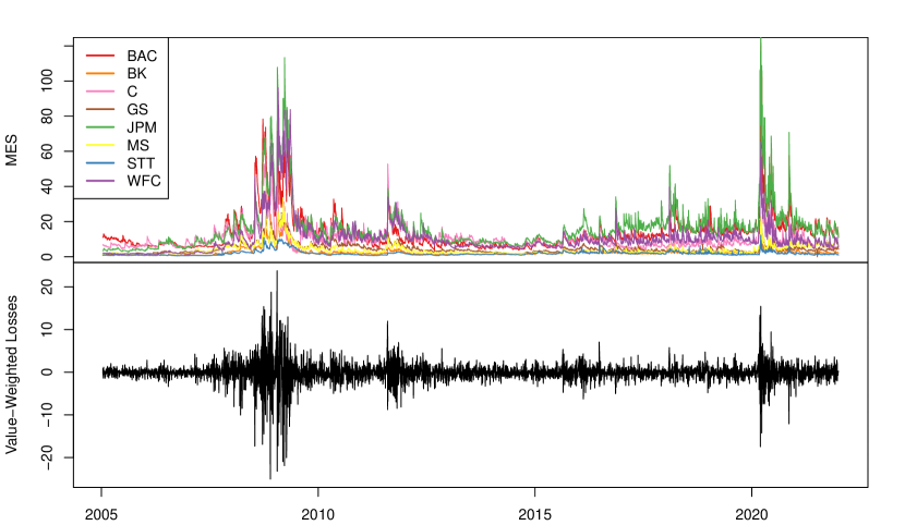
Figure 1: Top panel: Value-weighted MES forecasts for eight US G-SIBs Bank of America (BAC), Bank of New York Mellon (BK), Citigroup (C), Goldman Sachs (GS), JP Morgan Chase (JPM), Morgan Stanley (MS), State Street (STT), and Wells Fargo (WFC). Bottom panel: Time series of value-weighted losses $X_{t}$.

From a regulatory perspective, it is important—at each point $t$ in time—to limit the risk of the overall banking system as measured by the ES, viz.

$$\operatorname{E}[X_{t}\mid X_{t}>\operatorname{VaR}_{t}(p),\mathcal{F}_{t-1}]=\sum_{d=1}^{D}w_{t-1,d}\operatorname{E}[Y_{t,d}\mid X_{t}>\operatorname{VaR}_{t}(p),\mathcal{F}_{t-1}]=\sum_{d=1}^{D}w_{t-1,d}\theta_{t-1,p,d}.$$

The bottom panel of Figure 1 shows a plot of the value-weighted losses $X_{t}$. During periods of high volatility, aggregate risk of the system is high. Such periods are noticeable during the financial crisis of 2007–2009, the European sovereign debt crisis in the early 2010s, and the Corona crash of March 2020.

The top panel of Figure 1 plots the systemic risk contributions of each bank as measured by the value-weighted MES $w_{t-1,d}\theta_{t-1,p,d}$. Clearly, the contributions vary through time. Notice also that the MES forecasts during 2021 largely reflect the systemic risk contributions of the different institutions as determined by the FSB (2021). For instance, JP Morgan Chase is listed as the systemically most risky bank by the FSB (2021), which is mirrored by the high MES forecasts in the top panel of Figure 1. At the other end of the spectrum, State Street, Bank of New York Mellon, and Morgan Stanley are deemed least risky by the FSB (2021), similarly as their low MES forecasts suggest.

The placement of the institutions in different buckets by the FSB (2021) (with bucket 5 containing the most systemically risky institutions and bucket 1 the least systemically risky ones) suggests that the systemic risk contributions of the different banks may also be distinguishable in statistical terms. Thus, for each point in time $t$ for which MES forecasts are issued, we test equality of the value-weighted MES forecasts, i.e., $w_{t-1,1}\theta_{t-1,p,1}=\ldots=w_{t-1,D}\theta_{t-1,p,D}$. To do so, we use the test statistic $\mathcal{T}_{n}$ from Corollary 1. For each point in time, the $p$-value is virtually zero, indicating—as expected—large heterogeneity of systemic risk contributions among banks.

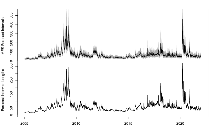
Figure 2: Top panel: MES forecasts (solid black line) together with 95%-confidence intervals (shaded grey area) for JP Morgan Chase. Bottom panel: Lengths of 95%-confidence intervals.

To limit the overall riskiness of the system, it seems prudent for the regulator to not only rely on the point MES forecasts, but also to take into account the estimation risk associated with those forecasts. To illustrate the significant impact of estimation risk, Figure 2 displays the MES forecasts together with the 95%-confidence intervals given in (10). It does so exemplarily for JP Morgan Chase, which is ranked as the world’s most systemically risky bank by the FSB (2021). The financial crisis of 2007–2009 and the Corona crash of March 2020 are associated with the largest spikes in systemic riskiness. It is precisely during these times, where precise risk assessments are needed most, that our intervals suggest that systemic riskiness is most poorly forecasted. This can be seen most clearly from the bottom panel of Figure 2, where lengths of the 95%-forecast intervals are shown. During crises (e.g., around 2008) the estimation risk in the forecasts is highest. In contrast, during calmer times, the estimation risk is comparatively smaller. Formula (10) suggests that the main driver of these differences in forecast quality is the volatility of the JP Morgan Chase shares.

7 Conclusion

For univariate risk measures, such as VaR and ES, there is a voluminous literature on asymptotic properties of forecasts. In contrast, asymptotic properties of systemic risk forecasts are largely unexplored. We fill this gap by deriving limit theory for EVT-based MES forecasts. In doing so, we extend the unconditional MES estimator of Cai et al. (2015) along two dimensions. First, we prove its validity when applied to residuals of multivariate volatility models, thus allowing it to be used for conditional MES forecasting and confidence interval construction. In simulations, we illustrate the good finite-sample coverage of the forecast intervals, which provide valuable information beyond the mere point forecast of MES. Second, we derive limit theory also in higher dimensional systems, therefore enabling joint inference on multiple MES forecasts. This may be beneficial as illustrated in the empirical application to the losses on the 8 US G-SIBs.

The following avenues may be worth exploring in future research. First, one may develop bootstrap-based confidence intervals for MES to improve coverage, particularly for not so extreme $p$. Second, it may be interesting to explore the properties of our forecasts for data-adaptive choices of $k$ and $k_{1}$, which may improve finite-sample properties. The results of Drees et al. (2020) in the context of extreme value index estimation suggest that this may influence the asymptotic behavior. Third, we have exclusively focused on MES as a measure of systemic risk in this paper. However, there are many other popular systemic risk measures in the literature, such as the CoVaR and CoES of Adrian and Brunnermeier (2016). Thus, future research could develop limit theory for (EVT-based) forecasts of these measures as well.

If not specified otherwise, all limits and all $o_{(\operatorname{P})}$- and $O_{(\operatorname{P})}$-symbols are to be interpreted with respect to $n\to\infty$. We denote by $K>0$ a large positive constant, that may change from line to line, and by $\bm{I}$ the identity matrix of appropriate dimension.

Appendix A Proof of Theorem 1

The proof of Theorem 1 requires Propositions 2 and 3.

Proposition 2.

Suppose Assumptions 1–3 hold, and the truncation sequence $\ell_{n}$ satisfies $\ell_{n}/\log n\to\infty$. Then, we have for any $\iota>0$ that, as $n\to\infty$,

$$\widehat{\bm{\varepsilon}}_{t}=\bm{\varepsilon}_{t}\big{\{}1+o_{\operatorname{P}}(n^{\iota-\xi})\big{\}},$$

$$\widehat{\bm{\sigma}}_{t}=\bm{\sigma}_{t}\big{\{}1+o_{\operatorname{P}}(n^{\iota-\xi})\big{\}}$$

uniformly in $t=1,\ldots,n+1$.

• See Appendix B. ∎

Proposition 3.

Under the conditions of Theorem 1, we have that, as $n\to\infty$,

$$\min\big{\{}\sqrt{k},\sqrt{k_{1}}/\log(d_{n})\big{\}}\log\Bigg{(}\frac{\widehat{\theta}_{p}}{\theta_{p}}\Bigg{)}\overset{d}{\longrightarrow}\begin{cases}\Theta+r\Gamma,&\text{if }r\leq 1,\\ (1/r)\Theta+\Gamma,&\text{if }r>1,\end{cases}$$

with $r$, $\Gamma$ and $\Theta$ defined as in Theorem 1.

• See Appendix C. ∎

• Use (2) and (9) to write

  $$\min \big{\{}\sqrt{k},\sqrt{k_{1}}/\log(d_{n})\big{\}}\log\Bigg{(}\frac{\widehat{\theta}_{n,p}}{\theta_{n,p}}\Bigg{)}$$

  $$=\min\big{\{}\sqrt{k},\sqrt{k_{1}}/\log(d_{n})\big{\}}\log\Bigg{(}\frac{\widehat{\sigma}_{n+1,Y}}{\sigma_{n+1,Y}}\cdot\frac{\widehat{\theta}_{p}}{\theta_{p}}\Bigg{)}$$

  $$=\min\big{\{}\sqrt{k},\sqrt{k_{1}}/\log(d_{n})\big{\}}\log\Bigg{(}\frac{\widehat{\sigma}_{n+1,Y}}{\sigma_{n+1,Y}}\Bigg{)}+\min\big{\{}\sqrt{k},\sqrt{k_{1}}/\log(d_{n})\big{\}}\log\Bigg{(}\frac{\widehat{\theta}_{p}}{\theta_{p}}\Bigg{)}.$$ (A.1)

  From Proposition 2 and Assumption 6 it follows that for $\iota<\xi-\widetilde{\alpha}$,

  $$\min\big{\{}\sqrt{k},\sqrt{k_{1}}/\log(d_{n})\big{\}}\log\Bigg{(}\frac{\widehat{\sigma}_{n+1,Y}}{\sigma_{n+1,Y}}\Bigg{)} =\min\big{\{}\sqrt{k},\sqrt{k_{1}}/\log(d_{n})\big{\}}\log\Big{(}1+o_{\operatorname{P}}(n^{\iota-\xi})\Big{)}$$

  $$=\min\big{\{}\sqrt{k},\sqrt{k_{1}}/\log(d_{n})\big{\}}o_{\operatorname{P}}(n^{\iota-\xi})$$

  $$=O(n^{\widetilde{\alpha}})o_{\operatorname{P}}(n^{\iota-\xi})$$

  $$=o_{\operatorname{P}}(n^{\widetilde{\alpha}+\iota-\xi})$$

  $$=o_{\operatorname{P}}(1),$$ (A.2)

  because $\log x\sim x-1$, $x\to 1$. For the second right-hand side term in (A.1) Proposition 3 applies. Overall, the conclusion follows. ∎

Appendix B Proof of Proposition 2

• Fix $\iota>0$. Choose $M>0$ from Assumption 2 sufficiently large, such that $1/M<\iota$. Recall the definition of $\mathcal{N}(\bm{\theta}^{\circ})$ from Assumption 2. For $\bm{\theta}\in\mathcal{N}(\bm{\theta}^{\circ})$, write

  $$\widehat{\bm{\varepsilon}}_{t}(\bm{\theta}) =\widehat{\bm{\varSigma}}_{t}^{-1}(\bm{\theta})(X_{t},Y_{t})^{\prime}=\widehat{\bm{\varSigma}}_{t}^{-1}(\bm{\theta})\bm{\varSigma}_{t}(\bm{\theta}^{\circ})\bm{\varepsilon}_{t}$$

  $$=\big{[}\bm{\varSigma}_{t}^{-1}(\bm{\theta})\widehat{\bm{\varSigma}}_{t}(\bm{\theta})\big{]}^{-1}\big{[}\bm{\varSigma}_{t}^{-1}(\bm{\theta}^{\circ})\bm{\varSigma}_{t}(\bm{\theta})\big{]}^{-1}\bm{\varepsilon}_{t}$$

  $$=\Big{\{}\bm{I}+\bm{\varSigma}_{t}^{-1}(\bm{\theta})\big{[}\widehat{\bm{\varSigma}}_{t}(\bm{\theta})-\bm{\varSigma}_{t}(\bm{\theta})\big{]}\Big{\}}^{-1}\Big{\{}\bm{I}+\bm{\varSigma}_{t}^{-1}(\bm{\theta}^{\circ})\big{[}\bm{\varSigma}_{t}(\bm{\theta})-\bm{\varSigma}_{t}(\bm{\theta}^{\circ})\big{]}\Big{\}}^{-1}\bm{\varepsilon}_{t}.$$ (B.1)

  Use Assumption 3 (where $C_{0}$ is random) to conclude that

  $$\max_{t=1,\ldots,n+1}\mathinner{\!\left\lVert\bm{\varSigma}_{t}^{-1}(\bm{\theta})\big{[}\widehat{\bm{\varSigma}}_{t}(\bm{\theta})-\bm{\varSigma}_{t}(\bm{\theta})\big{]}\right\rVert} \leq\max_{t=1,\ldots,n+1}\mathinner{\!\left\lVert\bm{\varSigma}_{t}^{-1}(\bm{\theta})\right\rVert}\max_{t=1,\ldots,n+1}\big{\|}\widehat{\bm{\varSigma}}_{t}(\bm{\theta})-\bm{\varSigma}_{t}(\bm{\theta})\big{\|}$$

  $$\leq CC_{0}\rho^{\ell_{n}}=o_{\operatorname{P}}(n^{-K})$$ (B.2)

  for any $K>0$, because

  $$\rho^{\ell_{n}} =\exp\Big{\{}\log\big{(}\rho^{(\ell_{n}/\log n)\log n}\big{)}\Big{\}}$$

  $$=\exp\Big{\{}\log(n)\log\big{(}\rho^{\ell_{n}/\log n}\big{)}\Big{\}}=\big{(}\exp\{\log n\}\big{)}^{\log\big{(}\rho^{\ell_{n}/\log n}\big{)}}$$

  $$=k^{\log\big{(}\rho^{\ell_{n}/\log n}\big{)}}=o\big{(}n^{-K}\big{)},$$

  since $\ell_{n}/\log n\to\infty$ by assumption, such that $\rho^{\ell_{n}/\log n}\to 0$ and, hence, $\log\big{(}\rho^{\ell_{n}/\log n}\big{)}\to-\infty$.

  For the second right-hand side term in (B.1), we obtain that

  $$\max_{t=1,\ldots,n+1}\Big{\|}\bm{\varSigma}_{t}^{-1}(\bm{\theta}^{\circ})\big{[}\bm{\varSigma}_{t}(\bm{\theta})-\bm{\varSigma}_{t}(\bm{\theta}^{\circ})\big{]}\Big{\|}\leq\max_{t=1,\ldots,n+1}\bigg{|}\frac{\sigma_{t,X}(\bm{\theta})-\sigma_{t,X}(\bm{\theta}^{\circ})}{\sigma_{t,X}(\bm{\theta}^{\circ})}\bigg{|}\\ +\max_{t=1,\ldots,n+1}\bigg{|}\frac{\sigma_{t,Y}(\bm{\theta})-\sigma_{t,Y}(\bm{\theta}^{\circ})}{\sigma_{t,Y}(\bm{\theta}^{\circ})}\bigg{|}.$$ (B.3)

  Consider the first term on the right-hand side of (B.3). Define $\dot{\sigma}_{t,X}(\bm{\theta})=\partial\sigma_{t,X}(\bm{\theta})/\partial\bm{\theta}$. Use the mean value theorem to deduce that for some $\bm{\theta}^{\ast}$ on the line connecting $\bm{\theta}$ and $\bm{\theta}^{\circ}$,

  $$\max_{t=1,\ldots,n+1}\bigg{|}\frac{\sigma_{t,X}(\bm{\theta})-\sigma_{t,X}(\bm{\theta}^{\circ})}{\sigma_{t,X}(\bm{\theta}^{\circ})}\bigg{|} =\max_{t=1,\ldots,n+1}\bigg{|}\frac{\dot{\sigma}_{t,X}(\bm{\theta}^{\ast})(\bm{\theta}-\bm{\theta}^{\circ})}{\sigma_{t,X}(\bm{\theta}^{\circ})}\bigg{|}$$

  $$=\max_{t=1,\ldots,n+1}\bigg{|}\frac{\dot{\sigma}_{t,X}(\bm{\theta}^{\ast})}{\sigma_{t,X}(\bm{\theta}^{\ast})}\cdot\frac{\sigma_{t,X}(\bm{\theta}^{\ast})}{\sigma_{t,X}(\bm{\theta}^{\circ})}\cdot(\bm{\theta}-\bm{\theta}^{\circ})\bigg{|}$$

  $$\leq\max_{t=1,\ldots,n+1}\bigg{\{}\sup_{\bm{\theta}\in\mathcal{N}(\bm{\theta}^{\circ})}\mathinner{\!\left\lVert\frac{\dot{\sigma}_{t,X}(\bm{\theta})}{\sigma_{t,X}(\bm{\theta})}\right\rVert}\cdot\sup_{\bm{\theta}\in\mathcal{N}(\bm{\theta}^{\circ})}\bigg{|}\frac{\sigma_{t,X}(\bm{\theta})}{\sigma_{t,X}(\bm{\theta}^{\circ})}\bigg{|}\bigg{\}}\mathinner{\!\left\lVert\bm{\theta}-\bm{\theta}^{\circ}\right\rVert}.$$ (B.4)

  We obtain that

  $$\operatorname{P} \bigg{\{}\max_{t=1,\ldots,n+1}\bigg{\{}\sup_{\bm{\theta}\in\mathcal{N}(\bm{\theta}^{\circ})}\mathinner{\!\left\lVert\frac{\dot{\sigma}_{t,X}(\bm{\theta})}{\sigma_{t,X}(\bm{\theta})}\right\rVert}\cdot\sup_{\bm{\theta}\in\mathcal{N}(\bm{\theta}^{\circ})}\bigg{|}\frac{\sigma_{t,X}(\bm{\theta})}{\sigma_{t,X}(\bm{\theta}^{\circ})}\bigg{|}\bigg{\}}>\varepsilon n^{\iota}\bigg{\}}$$

  $$\leq\sum_{t=1}^{n+1}\operatorname{P}\bigg{\{}\sup_{\bm{\theta}\in\mathcal{N}(\bm{\theta}^{\circ})}\mathinner{\!\left\lVert\frac{\dot{\sigma}_{t,X}(\bm{\theta})}{\sigma_{t,X}(\bm{\theta})}\right\rVert}\cdot\sup_{\bm{\theta}\in\mathcal{N}(\bm{\theta}^{\circ})}\bigg{|}\frac{\sigma_{t,X}(\bm{\theta})}{\sigma_{t,X}(\bm{\theta}^{\circ})}\bigg{|}>\varepsilon n^{\iota}\bigg{\}}$$

  $$\leq\sum_{t=1}^{n+1}\frac{1}{\varepsilon^{M}n^{M\iota}}\operatorname{E}\bigg{[}\sup_{\bm{\theta}\in\mathcal{N}(\bm{\theta}^{\circ})}\mathinner{\!\left\lVert\frac{\dot{\sigma}_{t,X}(\bm{\theta})}{\sigma_{t,X}(\bm{\theta})}\right\rVert}^{M}\cdot\sup_{\bm{\theta}\in\mathcal{N}(\bm{\theta}^{\circ})}\bigg{|}\frac{\sigma_{t,X}(\bm{\theta})}{\sigma_{t,X}(\bm{\theta}^{\circ})}\bigg{|}^{M}\bigg{]}$$

  $$\leq\sum_{t=1}^{n+1}\frac{1}{\varepsilon^{M}n^{M\iota}}\Bigg{\{}\operatorname{E}\bigg{[}\sup_{\bm{\theta}\in\mathcal{N}(\bm{\theta}^{\circ})}\mathinner{\!\left\lVert\frac{\dot{\sigma}_{t,X}(\bm{\theta})}{\sigma_{t,X}(\bm{\theta})}\right\rVert}^{Mp_{\ast}}\Bigg{\}}^{1/p_{\ast}}\cdot\Bigg{\{}\operatorname{E}\bigg{[}\sup_{\bm{\theta}\in\mathcal{N}(\bm{\theta}^{\circ})}\bigg{|}\frac{\sigma_{t,X}(\bm{\theta})}{\sigma_{t,X}(\bm{\theta}^{\circ})}\bigg{|}^{Mq_{\ast}}\bigg{]}\Bigg{\}}^{1/q_{\ast}}$$

  $$\leq Kn^{1-M\iota},$$

  where we used subadditivity in the first step, Markov’s inequality in the second step, Hölder’s inequality in the third step, and Assumption 2 for the final inequality. Therefore, since $1/M<\iota$,

  $$\max_{t=1,\ldots,n+1}\bigg{\{}\sup_{\bm{\theta}\in\mathcal{N}(\bm{\theta}^{\circ})}\mathinner{\!\left\lVert\frac{\dot{\sigma}_{t,X}(\bm{\theta})}{\sigma_{t,X}(\bm{\theta})}\right\rVert}\cdot\sup_{\bm{\theta}\in\mathcal{N}(\bm{\theta}^{\circ})}\bigg{|}\frac{\sigma_{t,X}(\bm{\theta})}{\sigma_{t,X}(\bm{\theta}^{\circ})}\bigg{|}\bigg{\}}=o_{\operatorname{P}}(n^{\iota}),$$

  whence from (B.4) and Assumption 1,

  $$\max_{t=1,\ldots,n+1}\bigg{|}\frac{\sigma_{t,X}(\bm{\theta})-\sigma_{t,X}(\bm{\theta}^{\circ})}{\sigma_{t,X}(\bm{\theta}^{\circ})}\bigg{|}=o_{\operatorname{P}}(n^{\iota})n^{-\xi}n^{\xi}\mathinner{\!\left\lVert\bm{\theta}-\bm{\theta}^{\circ}\right\rVert}=o_{\operatorname{P}}(n^{\iota-\xi})O_{\operatorname{P}}(1)=o_{\operatorname{P}}(n^{\iota-\xi}).$$ (B.5)

  Using identical arguments, we may also show that

  $$\max_{t=1,\ldots,n+1}\bigg{|}\frac{\sigma_{t,Y}(\bm{\theta})-\sigma_{t,Y}(\bm{\theta}^{\circ})}{\sigma_{t,Y}(\bm{\theta}^{\circ})}\bigg{|}=o_{\operatorname{P}}(n^{\iota-\xi}).$$

  Thus, from (B.3),

  $$\max_{t=1,\ldots,n+1}\mathinner{\!\left\lVert\bm{\varSigma}_{t}^{-1}(\bm{\theta}^{\circ})\big{[}\bm{\varSigma}_{t}(\bm{\theta})-\bm{\varSigma}_{t}(\bm{\theta}^{\circ})\big{]}\right\rVert}=o_{\operatorname{P}}(n^{\iota-\xi}).$$ (B.6)

  Plugging (B.2) and (B.6) into (B.1), we get that for all $\bm{\theta}\in\mathcal{N}(\bm{\theta}^{\circ})$

  $$\widehat{\bm{\varepsilon}}_{t}(\bm{\theta})=\bm{\varepsilon}_{t}\big{\{}1+o_{\operatorname{P}}(n^{\iota-\xi})\big{\}},$$

  where we recall that the matrices $\bm{\varSigma}(\cdot)$ and $\widehat{\bm{\varSigma}}(\cdot)$ in (B.1) are diagonal. Since, by Assumption 1, $\widehat{\bm{\theta}}$ is an element of $\mathcal{N}(\bm{\theta}^{\circ})$ with probability approaching 1, as $n\to\infty$, the conclusion for the residuals follows.

  The uniform approximability of the volatilities follows from

  $$\bigg{|}\frac{\widehat{\sigma}_{t,X}(\bm{\theta})}{\sigma_{t,X}(\bm{\theta}^{\circ})}-1\bigg{|} =\bigg{|}\frac{\widehat{\sigma}_{t,X}(\bm{\theta})-\sigma_{t,X}(\bm{\theta})}{\sigma_{t,X}(\bm{\theta}^{\circ})}+\frac{\sigma_{t,X}(\bm{\theta})}{\sigma_{t,X}(\bm{\theta}^{\circ})}-1\bigg{|}$$

  $$\leq\bigg{|}\frac{\widehat{\sigma}_{t,X}(\bm{\theta})-\sigma_{t,X}(\bm{\theta})}{\sigma_{t,X}(\bm{\theta}^{\circ})}\bigg{|}+\bigg{|}\frac{\sigma_{t,X}(\bm{\theta})}{\sigma_{t,X}(\bm{\theta}^{\circ})}-1\bigg{|}$$

  $$=o_{\operatorname{P}}(n^{-K})+o_{\operatorname{P}}(n^{\iota-\xi})$$

  (from (B.2) and (B.5)) together with the $n^{\xi}$-consistency of $\widehat{\bm{\theta}}$ (from Assumption 1). A similar result obtains for $\widehat{\sigma}_{t,Y}$. ∎

Appendix C Proof of Proposition 3

Let $F_{+}(\cdot)$ denote the d.f. of $\varepsilon_{t,Y}^{+}$, and set $U_{+}=[1/(1-F_{+})]^{\leftarrow}$. Then, the proof of Theorem 2 in Cai et al. (2015) shows that Assumptions 4 and 5 (phrased in terms of $(\varepsilon_{t,X},\varepsilon_{t,Y})^{\prime}$) continue to hold for $(\varepsilon_{t,X},\varepsilon_{t,Y}^{+})^{\prime}$ with the same constants and functions $A_{i}(\cdot)$. This will be exploited in some of the following proofs without further mention.

For $(x,y)^{\prime}\in[0,\infty]^{2}\setminus\{(\infty,\infty)^{\prime}\}$, we define

$$R_{n}(x,y) =\frac{n}{k}\operatorname{P}\big{\{}F_{0}(\varepsilon_{t,X})>1-kx/n,\ F_{+}(\varepsilon_{t,Y}^{+})>1-ky/n\big{\}},$$

$$T_{n}(x,y) =\frac{1}{k}\sum_{t=1}^{n}I_{\big{\{}F_{0}(\varepsilon_{t,X})>1-kx/n,\ F_{+}(\varepsilon_{t,Y}^{+})>1-ky/n\big{\}}},$$

$$\widehat{T}_{n}(x,y) =\frac{1}{k}\sum_{t=1}^{n}I_{\big{\{}F_{0}(\widehat{\varepsilon}_{t,X})>1-kx/n,\ F_{+}(\widehat{\varepsilon}_{t,Y}^{+})>1-ky/n\big{\}}}.$$

The limit distribution of $\widehat{\theta}_{p}$ is characterized by the zero-mean Gaussian process

$$\big{\{}W_{R}(x,y)\big{\}}_{(x,y)^{\prime}\in[0,\infty]^{2}\setminus\{(\infty,\infty)^{\prime}\}}$$

with covariance structure given by

$$\operatorname{E}\big{[}W_{R}(x_{1},y_{1})W_{R}(x_{2},y_{2})\big{]}=R(x_{1}\wedge x_{2},y_{1}\wedge y_{2}).$$

Then,

$$\Theta =(\gamma_{1}-1)W_{R}(1,\infty)+\Big{\{}\int_{0}^{\infty}R(1,s)\,\mathrm{d}s^{-\gamma_{1}}\Big{\}}^{-1}\int_{0}^{\infty}W_{R}(1,s)\,\mathrm{d}s^{-\gamma_{1}},$$

$$\Gamma =\frac{\gamma_{1}}{\sqrt{q}}\Big{\{}-W_{R}(\infty,q)+\int_{0}^{q}s^{-1}W_{R}(\infty,s)\,\mathrm{d}s\Big{\}}$$

are the zero-mean Gaussian random variables from Theorem 1.

The proof of Proposition 3 requires Lemmas 1–3. These lemmas build on Proposition 3.1 in Einmahl et al. (2006). Invoking a Skorohod construction, the limit processes involved in that proposition may be assumed to be defined on the same probability space. This leads to an easier presentation of some of the subsequent results. We state the version of Proposition 3.1 as given in Cai et al. (2015, Lemma 1):

Lemma 1.

Suppose that (4) holds. Then, for any $\eta\in[0,1/2)$ and $T>0$, it holds that, as $n\to\infty$,

$$\sup_{x,y\in(0,T]} y^{-\eta}\Big{|}\sqrt{k}\big{\{}T_{n}(x,y)-R_{n}(x,y)\big{\}}-W_{R}(x,y)\Big{|}\overset{a.s.}{\longrightarrow}0,$$

$$\sup_{x\in(0,T]} x^{-\eta}\Big{|}\sqrt{k}\big{\{}T_{n}(x,\infty)-x\big{\}}-W_{R}(x,\infty)\Big{|}\overset{a.s.}{\longrightarrow}0,$$ (C.1)

$$\sup_{y\in(0,T]} y^{-\eta}\Big{|}\sqrt{k}\big{\{}T_{n}(\infty,y)-y\big{\}}-W_{R}(\infty,y)\Big{|}\overset{a.s.}{\longrightarrow}0.$$

Lemma 2.

Under the conditions of Theorem 1, we have that, as $n\to\infty$,

$$\sqrt{k_{1}}\big{(}\widehat{\gamma}_{1}-\gamma_{1}\big{)}\overset{\operatorname{P}}{\longrightarrow}\Gamma.$$

• See Appendix D. ∎

For the next lemma, we introduce the following (with the exception of $\widehat{\theta}_{k/n}$) infeasible estimators of $\theta_{k/n}$:

$$\widetilde{\theta}_{k/n} =\frac{1}{k}\sum_{t=1}^{n}\varepsilon_{t,Y}^{+}I_{\big{\{}\varepsilon_{t,X}>\varepsilon_{(k+1),X}\big{\}}},$$

$$\widetilde{\theta}_{k/n}^{\ast} =\frac{1}{k}\sum_{t=1}^{n}\varepsilon_{t,Y}^{+}I_{\big{\{}\varepsilon_{t,X}>U_{0}(n/k)\big{\}}},$$

$$\widehat{\theta}_{k/n} =\frac{1}{k}\sum_{t=1}^{n}\widehat{\varepsilon}_{t,Y}^{+}I_{\big{\{}\widehat{\varepsilon}_{t,X}>\widehat{\varepsilon}_{(k+1),X}\big{\}}},$$

$$\widehat{\theta}_{k/n}^{\ast} =\frac{1}{k}\sum_{t=1}^{n}\widehat{\varepsilon}_{t,Y}^{+}I_{\big{\{}\widehat{\varepsilon}_{t,X}>U_{0}(n/k)\big{\}}}.$$

Moreover, define

$$e_{n} =(n/k)\big{\{}1-F_{0}(\varepsilon_{(k+1),X})\big{\}},$$ (C.2)

$$\widehat{e}_{n} =(n/k)\big{\{}1-F_{0}(\widehat{\varepsilon}_{(k+1),X})\big{\}},$$ (C.3)

such that $\widehat{e}_{n}\widehat{\theta}_{k\widehat{e}_{n}/n}^{\ast}=\widehat{\theta}_{k/n}$ and $e_{n}\widetilde{\theta}^{\ast}_{ke_{n}/n}=\widetilde{\theta}_{k/n}$.

Lemma 3.

Under the conditions of Theorem 1, we have that, as $n\to\infty$,

$$\frac{\sqrt{k}}{U_{1}(n/k)}\big{(}\widehat{\theta}_{k/n}-\widetilde{\theta}_{k/n}\big{)}=o_{\operatorname{P}}(1).$$

• See Appendix D. ∎

Now, we can prove Proposition 3.

• Write

  $$\frac{\widehat{\theta}_{p}}{\theta_{p}}=\frac{d_{n}^{\widehat{\gamma}_{1}}}{d_{n}^{\gamma_{1}}}\cdot\frac{\widehat{\theta}_{k/n}}{\theta_{k/n}^{+}}\cdot\frac{d_{n}^{\gamma_{1}}\theta_{k/n}^{+}}{\theta_{p}^{+}}\cdot\frac{\theta_{p}^{+}}{\theta_{p}}=\mathrel{\mathop{\mathchar 58\relax}}B_{1}\cdot B_{2}\cdot B_{3}\cdot B_{4}.$$

  First consider $B_{1}$. By the mean value theorem and $(\partial/\partial x)d^{x}=d^{x}\log d$, there exists $\vartheta\in(0,1)$, such that

  $$\frac{\sqrt{k_{1}}}{\log d_{n}}(B_{1}-1) =\frac{\sqrt{k_{1}}}{\log d_{n}}(d_{n}^{\widehat{\gamma}_{1}-\gamma_{1}}-d_{n}^{0})$$

  $$=\frac{\sqrt{k_{1}}}{\log d_{n}}d_{n}^{\vartheta(\widehat{\gamma}_{1}-\gamma_{1})}\log(d_{n})(\widehat{\gamma}_{1}-\gamma_{1})$$

  $$=\sqrt{k_{1}}(\widehat{\gamma}_{1}-\gamma_{1})\exp\big{\{}\log\big{(}d_{n}^{\vartheta(\widehat{\gamma}_{1}-\gamma_{1})}\big{)}\big{\}}$$

  $$=\sqrt{k_{1}}(\widehat{\gamma}_{1}-\gamma_{1})\exp\big{\{}\vartheta(\widehat{\gamma}_{1}-\gamma_{1})\log d_{n}\big{\}}$$

  $$=\sqrt{k_{1}}(\widehat{\gamma}_{1}-\gamma_{1})\big{\{}1+o_{\operatorname{P}}(1)\big{\}}$$

  $$=\Gamma+o_{\operatorname{P}}(1),$$ (C.4)

  where the second-to-last line follows from $\vartheta(\widehat{\gamma}_{1}-\gamma_{1})\log d_{n}=O_{\operatorname{P}}(\log d_{n}/\sqrt{k_{1}})=o_{\operatorname{P}}(1)$ (from Lemma 2 and our assumption that $\log d_{n}/\sqrt{k_{1}}=o(1)$), and the final line follows from Lemma 2.

  Combine our Lemma 3 with Proposition 3 in Cai et al. (2015) to get that

  $$\sqrt{k}(B_{2}-1)=\sqrt{k}\Bigg{(}\frac{\widehat{\theta}_{k/n}}{\theta_{k/n}^{+}}-1\Bigg{)}\overset{\operatorname{P}}{\longrightarrow}\Theta.$$

  Equation (32) of Cai et al. (2015) yields that

  $$B_{3}=1+o\big{(}1/\sqrt{k}\big{)}.$$

  Finally, the proof of Theorem 2 in Cai et al. (2015) shows that

  $$B_{4}=1+o\big{(}1/\sqrt{k}\big{)}.$$

  The rest of the proof follows as that of Theorem 1 in Cai et al. (2015). We give it here for the sake of completeness. Combining the above displays leads to

  $$\frac{\widehat{\theta}_{p}}{\theta_{p}}-1=B_{1}\cdot B_{2}\cdot B_{3}\cdot B_{4}-1$$

  $$=\bigg{[}1+\frac{\log d_{n}}{\sqrt{k_{1}}}\Gamma+o_{\operatorname{P}}\Big{(}\frac{\log d_{n}}{\sqrt{k_{1}}}\Big{)}\bigg{]}\bigg{[}1+\frac{\Theta}{\sqrt{k}}+o_{\operatorname{P}}\Big{(}\frac{1}{\sqrt{k}}\Big{)}\bigg{]}\bigg{[}1+o\Big{(}\frac{1}{\sqrt{k}}\Big{)}\bigg{]}\bigg{[}1+o\Big{(}\frac{1}{\sqrt{k}}\Big{)}\bigg{]}-1$$

  $$=\frac{\log d_{n}}{\sqrt{k_{1}}}\Gamma+\frac{\Theta}{\sqrt{k}}+o_{\operatorname{P}}\Big{(}\frac{\log d_{n}}{\sqrt{k_{1}}}\Big{)}+o_{\operatorname{P}}\Big{(}\frac{1}{\sqrt{k}}\Big{)}.$$ (C.5)

  Since $\log x\sim x-1$ as $x\to 1$, the claimed convergence follows. The variances and covariances of $\Gamma$ and $\Theta$ can be computed by using their definition and exploiting the covariance structure of $W_{R}(\cdot,\cdot)$ together with Fubini’s theorem. ∎

Appendix D Proofs of Lemmas 2–3

Define

$$s_{n}(y)=s_{n,k_{1}}(y)=\frac{n}{k_{1}}\Big{[}1-F_{+}\big{(}y^{-\gamma_{1}}U_{+}(n/k_{1})\big{)}\Big{]},\qquad y>0.$$

• As a first step, we show that for any $T>0$

  $$\sup_{y\in(0,T]}\Big{|}\frac{s_{n}(y)}{y}-1\Big{|}=o\big{(}1/\sqrt{k_{1}}\big{)}.$$ (D.1)

  Since $U_{1}(s)=U_{+}(s)$ for $s>1/\{1-F_{1}(0)\}$, we have from Assumption 5 that for any $y_{0}>0$,

  $$\sup_{y\geq y_{0}}\Big{|}y^{-\gamma_{1}}\frac{U_{+}(sy)}{U_{+}(s)}-1\Big{|}=O\{A_{1}(s)\},\qquad s\to\infty.$$

  Insert $s=n/k_{1}$ and $y=1/s_{n}(y)$ in that relation to obtain that

  $$\sup_{y\in(0,T]}\bigg{|}\Big{(}\frac{s_{n}(y)}{y}\Big{)}^{\gamma_{1}}-1\bigg{|}=O\{A_{1}(n/k_{1})\},\qquad n\to\infty.$$

  From $A_{1}(n/k_{1})=o\big{(}1/\sqrt{k_{1}}\big{)}$ by Assumption 6 and from a Taylor expansion, (D.1) follows.

Lemma 1 implies for any $\eta\in[0,1/2)$ and any $T>0$ that

$$\sup_{y\in(0,T]}y^{-\eta}\Big{|}\sqrt{k}\big{\{}T_{n}(\infty,y)-y\big{\}}-W_{R}(\infty,y)\Big{|}\overset{a.s.}{\longrightarrow}0.$$ (D.2)

Since $k_{1}/k\to q\in(0,\infty)$, we may replace $y$ by $y(k_{1}/k)$ in that relation to obtain

$$\sup_{y\in(0,T]}\Big{(}y\frac{k_{1}}{k}\Big{)}^{-\eta}\bigg{|}\sqrt{k}\Big{\{}\frac{1}{k}\sum_{t=1}^{n}I_{\big{\{}F_{+}(\varepsilon_{t,Y}^{+})>1-k_{1}y/n\big{\}}}-y\frac{k_{1}}{k}\Big{\}}-W_{R}\Big{(}\infty,y\frac{k_{1}}{k}\Big{)}\bigg{|}\overset{a.s.}{\longrightarrow}0$$

or, multiplying through with $\sqrt{k/k_{1}}$,

$$\sup_{y\in(0,T]}y^{-\eta}\Big{(}\frac{k_{1}}{k}\Big{)}^{-\eta}\bigg{|}\sqrt{k_{1}}\Big{\{}\frac{1}{k_{1}}\sum_{t=1}^{n}I_{\big{\{}F_{+}(\varepsilon_{t,Y}^{+})>1-k_{1}y/n\big{\}}}-y\Big{\}}-\sqrt{\frac{k_{1}}{k}}W_{R}\Big{(}\infty,y\frac{k_{1}}{k}\Big{)}\bigg{|}\overset{a.s.}{\longrightarrow}0.$$

Again, since $k_{1}/k\to q\in(0,\infty)$, we may drop the term $(k_{1}/k)^{-\eta}$ to get that

$$\sup_{y\in(0,T]}y^{-\eta}\bigg{|}\sqrt{k_{1}}\Big{\{}\frac{1}{k_{1}}\sum_{t=1}^{n}I_{\big{\{}F_{+}(\varepsilon_{t,Y}^{+})>1-k_{1}y/n\big{\}}}-y\Big{\}}-\sqrt{\frac{k_{1}}{k}}W_{R}\Big{(}\infty,y\frac{k_{1}}{k}\Big{)}\bigg{|}\overset{a.s.}{\longrightarrow}0.$$

Due to the uniform continuity of the weighted Wiener process,

$$\sup_{y\in(0,T]}y^{-\eta}\bigg{|}\sqrt{\frac{k}{k_{1}}}W_{R}\Big{(}\infty,y\frac{k_{1}}{k}\Big{)}-\frac{1}{\sqrt{q}}W_{R}(\infty,yq)\bigg{|}\overset{a.s.}{\longrightarrow}0.$$

The last two displays imply that

$$\sup_{y\in(0,T]}y^{-\eta}\bigg{|}\sqrt{k_{1}}\Big{\{}\frac{1}{k_{1}}\sum_{t=1}^{n}I_{\big{\{}F_{+}(\varepsilon_{t,Y}^{+})>1-k_{1}y/n\big{\}}}-y\Big{\}}-q^{-1/2}W_{R}(\infty,qy)\bigg{|}\overset{a.s.}{\longrightarrow}0.$$ (D.3)

With this and $s_{n}(y)\to y$, as $n\to\infty$, uniformly in $y\in(0,T]$ from (D.1), it follows for any $0<T_{1}<T$ that

$$\sup_{y\in(0,T_{1}]}s_{n}^{-\eta}(y)\bigg{|}\sqrt{k_{1}}\Big{\{}\frac{1}{k_{1}}\sum_{t=1}^{n}I_{\big{\{}\varepsilon_{t,Y}^{+}>y^{-\gamma_{1}}U_{+}(n/k_{1})\big{\}}}-s_{n}(y)\Big{\}}-q^{-1/2}W_{R}\{\infty,qs_{n}(y)\}\bigg{|}\overset{a.s.}{\longrightarrow}0.$$ (D.4)

Our next goal is to show that $s_{n}(y)$ can be replaced by $y$ at all three appearances in (D.4). From (D.1) it follows that, without changing the limit, $s_{n}(y)$ may be replaced by $y$ in (D.4) at the first two appearances. Finally, the uniform continuity of the weighted Wiener process ensures that, as $n\to\infty$,

$$\sup_{y\in(0,T_{1}]}y^{-\eta}q^{-1/2}\big{|}W_{R}\{\infty,qs_{n}(y)\}-W_{R}(\infty,qy)\big{|}\overset{a.s.}{\longrightarrow}0.$$

Thus, since $T$ and $T_{1}<T$ can be chosen arbitrarily large, we get for any $y_{0}>0$ that

$$\sup_{y\geq y_{0}}y^{\eta/\gamma_{1}}\bigg{|}\sqrt{k_{1}}\Big{\{}\frac{1}{k_{1}}\sum_{t=1}^{n}I_{\big{\{}\varepsilon_{t,Y}^{+}>yU_{+}(n/k_{1})\big{\}}}-y^{-1/\gamma_{1}}\Big{\}}-q^{-1/2}W_{R}\big{(}\infty,qy^{-1/\gamma_{1}}\big{)}\bigg{|}\overset{a.s.}{\longrightarrow}0.$$

Because $U_{+}(n/k_{1})=U_{1}(n/k_{1})>0$ for sufficiently large $n$, we get from this that

$$\sup_{y\geq y_{0}}y^{\eta/\gamma_{1}}\Big{|}\sqrt{k_{1}}\big{\{}T_{n}(y)-y^{-1/\gamma_{1}}\big{\}}-q^{-1/2}W_{R}\big{(}\infty,qy^{-1/\gamma_{1}}\big{)}\Big{|}\overset{a.s.}{\longrightarrow}0,$$ (D.5)

where $T_{n}(y)=\frac{1}{k_{1}}\sum_{t=1}^{n}I_{\big{\{}\varepsilon_{t,Y}>yU_{1}(n/k_{1})\big{\}}}$.

Our next goal is to show that $T_{n}(y)$ in (D.5) can be replaced by $\widehat{T}_{n}(y)=\frac{1}{k_{1}}\sum_{t=1}^{n}I_{\big{\{}\widehat{\varepsilon}_{t,Y}>yU_{1}(n/k_{1})\big{\}}}$. To task this, let $\delta_{n}=n^{\iota-\xi}$ with $\iota>0$ chosen sufficiently small to ensure that $\sqrt{k_{1}}\delta_{n}=o(1)$ (which is possible due to the Assumption 6 requirement that $\sqrt{k_{1}}=O(n^{\widetilde{\alpha}})$). By Proposition 2, $\widehat{\varepsilon}_{t,Y}=\varepsilon_{t,Y}\big{\{}1+o_{\operatorname{P}}\big{(}n^{\iota-\xi}\big{)}\big{\}}$ uniformly in $t=1,\ldots,n$. Thus, since $U_{1}(n/k_{1})>0$ for sufficiently large $n$ (by Assumption 5),

$$I_{\big{\{}\varepsilon_{t,Y}>(1+\delta_{n})yU_{1}(n/k_{1})\big{\}}}\leq I_{\big{\{}\widehat{\varepsilon}_{t,Y}>yU_{1}(n/k_{1})\big{\}}}\leq I_{\big{\{}\varepsilon_{t,Y}>(1-\delta_{n})yU_{1}(n/k_{1})\big{\}}}$$

holds for all $t=1,\ldots,n$ with probability approaching 1 (w.p.a. 1), as $n\to\infty$. Hence, for any $\varepsilon>0$ we can ensure that $\operatorname{P}\{\mathcal{W}_{1}\}>1-\varepsilon/3$ for sufficiently large $n$, where

$$\mathcal{W}_{1}\mathrel{\mathop{\mathchar 58\relax}}=\Big{\{}T_{n}\big{\{}(1+\delta_{n})y\big{\}}-T_{n}(y)\leq\widehat{T}_{n}(y)-T_{n}(y)\leq T_{n}\big{\{}(1-\delta_{n})y\big{\}}-T_{n}(y)\Big{\}}.$$

We now show that

$$\sup_{y\geq y_{0}}y^{\eta/\gamma_{1}}\Big{|}\sqrt{k_{1}}\Big{[}T_{n}\big{\{}(1\pm\delta_{n})y\big{\}}-T_{n}(y)\Big{]}\Big{|}\overset{a.s.}{\longrightarrow}0.$$ (D.6)

We only show (D.6) for $T_{n}\big{\{}(1+\delta_{n})y\big{\}}$, as the proof for $T_{n}\big{\{}(1-\delta_{n})y\big{\}}$ is similar. Bound

$$\sup_{y\geq y_{0}} \,y^{\eta/\gamma_{1}}\Big{|}\sqrt{k_{1}}\Big{[}T_{n}\big{\{}(1+\delta_{n})y\big{\}}-T_{n}(y)\Big{]}\Big{|}$$

$$\leq\sup_{y\geq y_{0}}y^{\eta/\gamma_{1}}\Big{|}\sqrt{k_{1}}\Big{[}T_{n}\big{\{}(1+\delta_{n})y\big{\}}-(1+\delta_{n})^{-1/\gamma_{1}}y^{-1/\gamma_{1}}\Big{]}$$

$$\hskip 199.16928pt-q^{-1/2}W_{R}\big{(}\infty,q(1+\delta_{n})^{-1/\gamma_{1}}y^{-1/\gamma_{1}}\big{)}\Big{|}$$

$$\hskip 28.45274pt+\sup_{y\geq y_{0}}y^{\eta/\gamma_{1}}\Big{|}\sqrt{k_{1}}\big{[}T_{n}(y)-y^{-1/\gamma_{1}}\big{]}-q^{-1/2}W_{R}\big{(}\infty,qy^{-1/\gamma_{1}}\big{)}\Big{|}$$

$$\hskip 28.45274pt+\sup_{y\geq y_{0}}y^{\eta/\gamma_{1}}q^{-1/2}\Big{|}W_{R}\big{(}\infty,q(1+\delta_{n})^{-1/\gamma_{1}}y^{-1/\gamma_{1}}\big{)}-W_{R}\big{(}\infty,qy^{-1/\gamma_{1}}\big{)}\Big{|}$$

$$\hskip 28.45274pt+\sqrt{k_{1}}\sup_{y\geq y_{0}}y^{\eta/\gamma_{1}}\gamma_{1}^{-1}\big{\{}\delta_{n}+o(\delta_{n})\big{\}}y^{-1/\gamma_{1}}$$

$$=o(1),$$

where we used (D.5), the uniform continuity of the weighted Wiener process, and the fact that $\sqrt{k_{1}}\delta_{n}=o(1)$ by our choice of $\delta_{n}$. This proves (D.6).

Now, we may use (D.6) to conclude that for any $\delta>0$ it holds for sufficiently large $n$ that

$$\operatorname{P} \Big{\{}\sup_{y\geq y_{0}}y^{\eta/\gamma_{1}}\Big{|}\sqrt{k_{1}}\big{[}\widehat{T}_{n}(y)-T_{n}(y)\big{]}\Big{|}\geq\delta\Big{\}}$$

$$\leq\operatorname{P}\Big{\{}\sup_{y\geq y_{0}}y^{\eta/\gamma_{1}}\Big{|}\sqrt{k_{1}}\big{[}\widehat{T}_{n}(y)-T_{n}(y)\big{]}\Big{|}\geq\delta,\ \mathcal{W}_{1}\Big{\}}+\operatorname{P}\big{\{}\mathcal{W}_{1}^{C}\big{\}}$$

$$\leq\operatorname{P}\Big{\{}\sup_{y\geq y_{0}}y^{\eta/\gamma_{1}}\Big{|}\sqrt{k_{1}}\big{[}\widehat{T}_{n}\big{\{}(1+\delta_{n})y\big{\}}-T_{n}(y)\big{]}\Big{|}\geq\delta,\ \mathcal{W}_{1}\Big{\}}$$

$$\hskip 28.45274pt+\operatorname{P}\Big{\{}\sup_{y\geq y_{0}}y^{\eta/\gamma_{1}}\Big{|}\sqrt{k_{1}}\big{[}\widehat{T}_{n}\big{\{}(1-\delta_{n})y\big{\}}-T_{n}(y)\big{]}\Big{|}\geq\delta,\ \mathcal{W}_{1}\Big{\}}+\operatorname{P}\big{\{}\mathcal{W}_{1}^{C}\big{\}}$$

$$\leq\frac{\varepsilon}{3}+\frac{\varepsilon}{3}+\frac{\varepsilon}{3}=\varepsilon.$$

Combine this with (D.5) to obtain that

$$\sup_{y\geq y_{0}}y^{\eta/\gamma_{1}}\Big{|}\sqrt{k_{1}}\big{[}\widehat{T}_{n}(y)-y^{-1/\gamma_{1}}\big{]}-q^{-1/2}W_{R}\big{(}\infty,qy^{-1/\gamma_{1}}\big{)}\Big{|}=o_{\operatorname{P}}(1).$$

From this convergence it follows as in the proof of Corollary 1 in Hoga (2017) that

$$\sup_{y\geq y_{0}}y^{\eta/\gamma_{1}}\bigg{|}\sqrt{k_{1}}\bigg{[}\frac{1}{k_{1}}\sum_{t=1}^{n}I_{\big{\{}\widehat{\varepsilon}_{t,Y}>y\widehat{\varepsilon}_{(k_{1}+1),Y}\big{\}}}-y^{-1/\gamma_{1}}\bigg{]}\\ -q^{-1/2}\Big{[}W_{R}\big{(}\infty,qy^{-1/\gamma_{1}}\big{)}-y^{-1/\gamma_{1}}W_{R}(\infty,q)\Big{]}\bigg{|}=o_{\operatorname{P}}(1).$$

As in Hoga (2017, Example 4), we then obtain that

$$\sqrt{k_{1}}(\widehat{\gamma}_{1}-\gamma_{1}) =\sqrt{k_{1}}\int_{1}^{\infty}\Big{[}\frac{1}{k_{1}}\sum_{t=1}^{n}I_{\big{\{}\widehat{\varepsilon}_{t,Y}>y\widehat{\varepsilon}_{(k_{1}+1),Y}\big{\}}}-y^{-1/\gamma_{1}}\Big{]}\frac{\,\mathrm{d}y}{y}$$

$$\overset{\operatorname{P}}{\underset{(n\to\infty)}{\longrightarrow}}q^{-1/2}\int_{1}^{\infty}W_{R}(\infty,qy^{-1/\gamma_{1}})\frac{\,\mathrm{d}y}{y}-q^{-1/2}\int_{1}^{\infty}y^{-1/\gamma_{1}-1}\,\mathrm{d}y\cdot W_{R}(\infty,q)$$

$$=q^{-1/2}\gamma_{1}\int_{0}^{q}s^{-1}W_{R}(\infty,s)\,\mathrm{d}s-q^{-1/2}\gamma_{1}W_{R}(\infty,q)$$

$$=\Gamma,$$

where we used the substitution $s=qy^{-1/\gamma_{1}}$ in the third step. This ends the proof. ∎

The proof of Lemma 3 builds on the preliminary Lemmas 4–6. These require the following additional notation:

$$s_{n}^{\pm}(y) =s_{n,k}\big{(}y\{1\pm\delta_{n}\}^{-1/\gamma_{1}}\big{)},$$

$$r_{n}^{\pm}(x) =\frac{n}{k}\Big{[}1-F_{0}\big{\{}(1\pm\delta_{n})U_{0}(n/[kx])\big{\}}\Big{]},$$ (D.7)

where $\delta_{n}=n^{\iota-\xi}$ as in the above proof of Lemma 2. Also let $s_{n}(y)=s_{n,k}(y)$ for brevity from now on.

Lemma 4.

Under Assumptions 5 and 6, it holds that, as $n\to\infty$,

$$\sup_{x\in[1/2,2]}\big{|}r_{n}^{\pm}(x)-x\big{|}=o\big{(}1/\sqrt{k}\big{)}.$$

• By the regular variation condition (5) and de Haan and Ferreira (2006, Theorem 1.2.1),

  $$\frac{r_{n}^{\pm}(x)}{x}=\frac{\frac{n}{k}\big{[}1-F_{0}\{(1\pm\delta_{n})U_{0}(n/[kx])\}\big{]}}{\frac{n}{k}\big{[}1-F_{0}\{U_{0}(n/[kx])\}\big{]}}\underset{(n\to\infty)}{\longrightarrow}(1\pm\delta_{n})^{-1/\gamma_{0}}.$$ (D.8)

  Moreover, Assumption 5 implies that there exists $t_{0}>0$ such that for $t>t_{0}$ and $u>1/2$,

  $$\Bigg{|}\frac{u^{-\gamma_{0}}U_{0}(tu)/U_{0}(t)-1}{A_{0}(t)}\Bigg{|}<K.$$

  Inserting $t=\frac{n}{kx}$ and $u=x/r_{n}^{\pm}(x)$ in that relation it follows that

  $$\Bigg{|}\frac{\Big{(}\frac{r_{n}^{\pm}(x)}{x}\Big{)}^{\gamma_{0}}(1\pm\delta_{n})-1}{A_{0}\big{(}\frac{n}{kx}\big{)}}\Bigg{|}<K.$$

  Multiplying through with $|A_{0}\big{(}\frac{n}{kx}\big{)}|$ gives

  $$\bigg{|}\Big{(}\frac{r_{n}^{\pm}(x)}{x}\Big{)}^{\gamma_{0}}-1\pm\delta_{n}\Big{(}\frac{r_{n}^{\pm}(x)}{x}\Big{)}^{\gamma_{0}}\Big{|}<K\Big{|}A_{0}\Big{(}\frac{n}{kx}\Big{)}\Big{|}.$$

  By (D.8), this implies

  $$\bigg{|}\Big{(}\frac{r_{n}^{\pm}(x)}{x}\Big{)}^{\gamma_{0}}-1\bigg{|}<K\bigg{[}\Big{|}A_{0}\Big{(}\frac{n}{kx}\Big{)}\Big{|}+\delta_{n}\bigg{]}.$$

  Use the Taylor expansion

  $$\Big{(}\frac{r_{n}^{\pm}(x)}{x}\Big{)}^{\gamma_{0}}-1=\gamma_{0}\Big{[}\frac{r_{n}^{\pm}(x)}{x}-1\Big{]}+o\Big{(}\frac{r_{n}^{\pm}(x)}{x}-1\Big{)}$$

  to deduce that

  $$\Big{|}\frac{r_{n}^{\pm}(x)}{x}-1\Big{|}<K\Bigg{[}\Big{|}A_{0}\Big{(}\frac{n}{kx}\Big{)}\Big{|}+\delta_{n}\Bigg{]}.$$

  By Assumption 6 and the Potter bounds (de Haan and Ferreira, 2006, Proposition B.1.9(5)), it holds for any $\delta>0$ and $n$ sufficiently large,

  $$\sqrt{k}\Big{|}A_{0}\Big{(}\frac{n}{kx}\Big{)}\Big{|} =\sqrt{k}\big{|}A_{0}(n/k)\big{|}\frac{A_{0}\big{(}n/[kx]\big{)}}{A_{0}(n/k)}$$

  $$=o(1)x^{-\rho_{0}}\max\{x^{\delta},\ x^{-\delta}\}=o(1)$$

  uniformly in $x\in(0,T]$. Since also $\sqrt{k}\delta_{n}=o(1)$ by Assumption 6, the conclusion follows. ∎

Lemma 5.

Under the conditions of Theorem 1, we have that, as $n\to\infty$,

$$\sup_{x\in[1/2,2]}\bigg{|}\frac{\sqrt{k}}{U_{1}(n/k)}\Big{[}x\widehat{\theta}^{\ast}_{kx/n}-x\widetilde{\theta}^{\ast}_{kx/n}\Big{]}\bigg{|}=o_{\operatorname{P}}(1).$$ (D.9)

• Using the substitution $s=U_{1}(n/k)y^{-\gamma_{1}}$, we get that

  $$-U_{1} (n/k)\int_{0}^{\infty}\widehat{T}_{n}\{x,s_{n}(y)\}\,\mathrm{d}y^{-\gamma_{1}}$$

  $$=-U_{1}(n/k)\int_{0}^{\infty}\frac{1}{k}\sum_{t=1}^{n}I_{\big{\{}F_{0}(\widehat{\varepsilon}_{t,X})>1-kx/n,\ F_{+}(\widehat{\varepsilon}_{t,Y}^{+})>F_{+}(y^{-\gamma_{1}}U_{+}(n/k))\big{\}}}\,\mathrm{d}y^{-\gamma_{1}}$$

  $$=-U_{1}(n/k)\frac{1}{k}\sum_{t=1}^{n}\int_{0}^{\infty}I_{\big{\{}\widehat{\varepsilon}_{t,X}>U_{0}(n/[kx]),\ \widehat{\varepsilon}_{t,Y}^{+}>y^{-\gamma_{1}}U_{+}(n/k)\big{\}}}\,\mathrm{d}y^{-\gamma_{1}}$$

  $$=\frac{1}{k}\sum_{t=1}^{n}\int_{0}^{\infty}I_{\big{\{}\widehat{\varepsilon}_{t,X}>U_{0}(n/[kx]),\ \widehat{\varepsilon}_{t,Y}^{+}>s\big{\}}}\,\mathrm{d}s$$

  $$=\frac{1}{k}\sum_{t=1}^{n}\int_{0}^{\widehat{\varepsilon}_{t,Y}^{+}}I_{\big{\{}\widehat{\varepsilon}_{t,X}>U_{0}(n/[kx])\big{\}}}\,\mathrm{d}s$$

  $$=\frac{1}{k}\sum_{t=1}^{n}\widehat{\varepsilon}_{t,Y}^{+}I_{\big{\{}\widehat{\varepsilon}_{t,X}>U_{0}(n/[kx])\big{\}}}$$

  $$=x\widehat{\theta}^{\ast}_{kx/n}.$$

  By similar arguments,

  $$x\widetilde{\theta}^{\ast}_{kx/n}=-U_{1}(n/k)\int_{0}^{\infty}T_{n}\big{\{}x,s_{n}(y)\big{\}}\,\mathrm{d}y^{-\gamma_{1}}.$$ (D.10)

  Thus, in view of (D.9), we only have to show that

  $$\sup_{x\in[1/2,2]}\Big{|}\sqrt{k}\int_{0}^{\infty}\Big{[}\widehat{T}_{n}\big{\{}x,s_{n}(y)\big{\}}-T_{n}\big{\{}x,s_{n}(y)\big{\}}\Big{]}\,\mathrm{d}y^{-\gamma_{1}}\Big{|}=o_{\operatorname{P}}(1).$$ (D.11)

  By our choice $\delta_{n}=n^{\iota-\xi}$ and Proposition 2, the following inequality holds w.p.a. 1, as $n\to\infty$,

  $$\widehat{T}_{n}\{x,s_{n}(y)\} =\frac{1}{k}\sum_{t=1}^{n}I_{\Big{\{}\widehat{\varepsilon}_{t,X}>U_{0}\big{(}\frac{n}{kx}\big{)},\ \widehat{\varepsilon}_{t,Y}^{+}>U_{+}\big{(}\frac{n}{ks_{n}(y)}\big{)}\Big{\}}}$$

  $$\leq\frac{1}{k}\sum_{t=1}^{n}I_{\Big{\{}\varepsilon_{t,X}>(1-\delta_{n})U_{0}\big{(}\frac{n}{kx}\big{)},\ \varepsilon_{t,Y}^{+}>(1-\delta_{n})U_{+}\big{(}\frac{n}{ks_{n}(y)}\big{)}\Big{\}}}$$

  $$=\frac{1}{k}\sum_{t=1}^{n}I_{\Big{\{}\varepsilon_{t,X}>U_{0}\big{(}\frac{n}{kr_{n}^{-}(x)}\big{)},\ \varepsilon_{t,Y}^{+}>U_{+}\big{(}\frac{n}{ks_{n}^{-}(y)}\big{)}\Big{\}}}$$

  $$=T_{n}\{r_{n}^{-}(x),\ s_{n}^{-}(y)\}.$$

  Similarly,

  $$\widehat{T}_{n}\{x,s_{n}(y)\}\geq T_{n}\{r_{n}^{+}(x),s_{n}^{+}(y)\}$$

  w.p.a. 1, as $n\to\infty$. Fix some arbitrary $\varepsilon>0$ and define

  $$\mathcal{W}_{2}\mathrel{\mathop{\mathchar 58\relax}}=\Big{\{}T_{n}\big{\{}r_{n}^{+}(x),s_{n}^{+}(y)\big{\}}-T_{n}\big{\{}x,s_{n}(y)\big{\}}\leq\widehat{T}_{n}\big{\{}x,s_{n}(y)\big{\}}-T_{n}\big{\{}x,s_{n}(y)\big{\}}\\ \leq T_{n}\big{\{}r_{n}^{-}(x),s_{n}^{-}(y)\big{\}}-T_{n}\big{\{}x,s_{n}(y)\big{\}}\Big{\}}.$$

  Then, by the above, $\operatorname{P}\{\mathcal{W}_{2}\}>1-\varepsilon$ for sufficiently large $n$. Thus, to prove (D.11) it suffices to show that

  $$\sup_{x\in[1/2,2]}\Big{|}\sqrt{k}\int_{0}^{\infty}\Big{[}T_{n}\big{\{}r_{n}^{\pm}(x),s_{n}^{\pm}(y)\big{\}}-T_{n}\big{\{}x,s_{n}(y)\big{\}}\Big{]}\,\mathrm{d}y^{-\gamma_{1}}\Big{|}=o_{\operatorname{P}}(1).$$

  We only do so for $T_{n}\{r_{n}^{+}(x),s_{n}^{+}(y)\}$, as the claim for $T_{n}\{r_{n}^{-}(x),s_{n}^{-}(y)\}$ can be established analogously. Decompose

  $$\sup_{x\in[1/2,2]} \Big{|}\sqrt{k}\int_{0}^{\infty}\Big{[}T_{n}\big{\{}r_{n}^{+}(x),s_{n}^{+}(y)\big{\}}-T_{n}\big{\{}x,s_{n}(y)\big{\}}\Big{]}\,\mathrm{d}y^{-\gamma_{1}}\Big{|}$$

  $$\leq\sup_{x\in[1/2,2]}\Big{|}\int_{0}^{\infty}\sqrt{k}\Big{[}T_{n}\big{\{}r_{n}^{+}(x),s_{n}^{+}(y)\big{\}}-R_{n}\big{\{}r_{n}^{+}(x),s_{n}^{+}(y)\big{\}}\Big{]}-W_{R}(x,y)\,\mathrm{d}y^{-\gamma_{1}}\Big{|}$$

  $$\hskip 28.45274pt+\sup_{x\in[1/2,2]}\Big{|}\int_{0}^{\infty}\sqrt{k}\Big{[}T_{n}\big{\{}x,s_{n}(y)\big{\}}-R_{n}\big{\{}x,s_{n}(y)\big{\}}\Big{]}-W_{R}(x,y)\,\mathrm{d}y^{-\gamma_{1}}\Big{|}$$

  $$\hskip 28.45274pt+\sup_{x\in[1/2,2]}\Big{|}\int_{0}^{\infty}\sqrt{k}\Big{[}R_{n}\big{\{}r_{n}^{+}(x),s_{n}^{+}(y)\big{\}}-R(x,y)\Big{]}\,\mathrm{d}y^{-\gamma_{1}}\Big{|}$$

  $$\hskip 28.45274pt+\sup_{x\in[1/2,2]}\Big{|}\int_{0}^{\infty}\sqrt{k}\Big{[}R_{n}\big{\{}x,s_{n}(y)\big{\}}-R(x,y)\Big{]}\,\mathrm{d}y^{-\gamma_{1}}\Big{|}$$

  $$=C_{1}+C_{2}+C_{3}+C_{4}.$$

  We show in turn that $C_{1},\ldots,C_{4}$ are asymptotically negligible.

  By (D.10) and the fact that similarly $x\theta_{kx/n}=-U_{1}(n/k)\int_{0}^{\infty}R_{n}\{x,s_{n}(y)\}\,\mathrm{d}y^{-\gamma_{1}}$,

  $$C_{2}=\sup_{x\in[1/2,2]}\bigg{|}\frac{\sqrt{k}}{U_{1}(n/k)}\big{[}x\widetilde{\theta}_{kx/n}^{\ast}-x\theta_{kx/n}\big{]}-\int_{0}^{\infty}W_{R}(x,y)\,\mathrm{d}y^{-\gamma_{1}}\bigg{|}.$$ (D.12)

  Thus, $C_{2}=o_{\operatorname{P}}(1)$ follows from Proposition 2 in Cai et al. (2015).

  Carefully reading the proof of that proposition reveals that $s_{n}(y)$ in (D.12) (appearing in both $x\widetilde{\theta}_{kx/n}^{\ast}$ and $x\theta_{kx/n}$) can be replaced by $s_{n}^{+}(y)$ without changing the conclusion that the term is $o_{\operatorname{P}}(1)$. This exploits the fact that $\sup_{y\in(0,1]}s_{n}(y)/y^{(\gamma_{1}+\eta_{1})}\to 0$ for $\eta_{1}>\gamma_{1}$ and $\sup_{y\in(0,T]}|s_{n}(y)-y|\to 0$ continue to hold for $s_{n}^{+}(y)$. Additionally using Lemma 4 we see that $x$ in (D.12) can be replaced by $r_{n}^{+}(x)$, such that

  $$\sup_{x\in[1/2,2]}\Big{|}\int_{0}^{\infty}\sqrt{k}\big{[}T_{n}\{r_{n}^{+}(x),s_{n}^{+}(y)\}-R_{n}\{r_{n}^{+}(x),s_{n}^{+}(y)\}\big{]}-W_{R}\{r_{n}^{+}(x),y\}\,\mathrm{d}y^{-\gamma_{1}}\Big{|}=o_{\operatorname{P}}(1).$$

  Hence, $C_{1}=o_{\operatorname{P}}(1)$ follows if we can show that

  $$\sup_{x\in[1/2,2]}\Big{|}\int_{0}^{\infty}W_{R}(x,y)-W_{R}\big{\{}r_{n}^{+}(x),y\big{\}}\,\mathrm{d}y^{-\gamma_{1}}\Big{|}=o_{\operatorname{P}}(1).$$ (D.13)

  By Corollary 1.11 of Adler (1990), $(x,y)\mapsto W_{R}(x,y)$ is continuous on $[1/2,2]\times(0,\infty)$. This implies that

  $$[1/2,2]\ni x\mapsto\int_{0}^{\infty}W_{R}(x,y)\,\mathrm{d}y^{-\gamma_{1}}$$

  is continuous and, hence, uniformly continuous on the bounded interval $[1/2,2]$. Thus, (D.13) follows from Lemma 4, showing that $C_{1}=o_{\operatorname{P}}(1)$.

  The fact that $C_{4}=o(1)$ follows directly from Cai et al. (2015, p. 439).

  To prove $C_{3}=o(1)$, consider the bound

  $$C_{3} \leq\sup_{x\in[1/2,2]}\Big{|}\int_{0}^{\infty}\sqrt{k}\Big{[}R_{n}\big{\{}r_{n}^{+}(x),s_{n}^{+}(y)\big{\}}-R\big{\{}r_{n}^{+}(x),y(1+\delta_{n})^{-1/\gamma_{1}}\big{\}}\Big{]}\,\mathrm{d}y^{-\gamma_{1}}\Big{|}$$

  $$\hskip 28.45274pt+\sup_{x\in[1/2,2]}\Big{|}\int_{0}^{\infty}\sqrt{k}\Big{[}R\big{\{}r_{n}^{+}(x),y(1+\delta_{n})^{-1/\gamma_{1}}\big{\}}-R\big{\{}r_{n}^{+}(x),y\big{\}}\Big{]}\,\mathrm{d}y^{-\gamma_{1}}\Big{|}$$

  $$\hskip 28.45274pt+\sup_{x\in[1/2,2]}\Big{|}\int_{0}^{\infty}\sqrt{k}\Big{[}R\big{\{}r_{n}^{+}(x),y\big{\}}-R(x,y)\Big{]}\,\mathrm{d}y^{-\gamma_{1}}\Big{|}$$

  $$=C_{31}+C_{32}+C_{33}.$$

  Recalling that $s_{n}^{+}(y)=s_{n}\{y(1+\delta_{n})^{-1/\gamma_{1}}\}$, we obtain by a change of variables that

  $$C_{31} =\sup_{x\in[1/2,2]}\Big{|}\int_{0}^{\infty}\sqrt{k}\Big{[}R_{n}\big{\{}r_{n}^{+}(x),s_{n}^{+}(y)\big{\}}-R\big{\{}r_{n}^{+}(x),y(1+\delta_{n})^{-1/\gamma_{1}}\big{\}}\Big{]}\,\mathrm{d}y^{-\gamma_{1}}\Big{|}$$

  $$=(1+\delta_{n})^{-1}\sup_{x\in[1/2,2]}\Big{|}\int_{0}^{\infty}\sqrt{k}\Big{[}R_{n}\big{\{}r_{n}^{+}(x),s_{n}(y)\big{\}}-R\big{\{}r_{n}^{+}(x),y\big{\}}\Big{]}\,\mathrm{d}y^{-\gamma_{1}}\Big{|}$$

  $$=o(1),$$

  where we used the fact that $C_{4}=o(1)$ together with Lemma 4 in the final step. For $C_{32}$ we again use a change of variables to obtain

  $$\int_{0}^{\infty}R\big{\{}r_{n}^{+}(x),y(1+\delta_{n})^{-1/\gamma_{1}}\big{\}}\,\mathrm{d}y^{-\gamma_{1}}=(1+\delta_{n})^{-1}\int_{0}^{\infty}R\big{\{}r_{n}^{+}(x),y\big{\}}\,\mathrm{d}y^{-\gamma_{1}}.$$

  Thus, since $(1+\delta_{n})^{-1}=1-\delta_{n}+o(\delta_{n})$ from a Taylor expansion,

  $$C_{32}\leq K\sqrt{k}\delta_{n}\sup_{x\in[1/2,2]}\int_{0}^{\infty}R\{r_{n}^{+}(x),y\}\,\mathrm{d}y^{-\gamma_{1}}=o(1).$$

  Finally, Schmidt and Stadtmüller (2006, Theorem 1 (ii)) establish homogeneity of the $R$-function, i.e., $R(sx,sy)=sR(x,y)$ for all $s>0$ and $x,y\geq 0$. Using this and a change of variables,

  $$\int_{0}^{\infty}\sqrt{k} \Big{[}R\big{\{}r_{n}^{+}(x),y\big{\}}-R(x,y)\Big{]}\,\mathrm{d}y^{-\gamma_{1}}$$

  $$=\sqrt{k}\bigg{[}\int_{0}^{\infty}R\big{\{}r_{n}^{+}(x),y\big{\}}\,\mathrm{d}y^{-\gamma_{1}}-\int_{0}^{\infty}R(x,y)\,\mathrm{d}y^{-\gamma_{1}}\bigg{]}$$

  $$=\sqrt{k}\bigg{[}\int_{0}^{\infty}r_{n}^{+}(x)R\big{\{}1,y/r_{n}^{+}(x)\big{\}}\,\mathrm{d}y^{-\gamma_{1}}-\int_{0}^{\infty}xR(1,y/x)\,\mathrm{d}y^{-\gamma_{1}}\bigg{]}$$

  $$=\sqrt{k}\big{[}r_{n}^{+}(x)^{1-\gamma_{1}}-x^{1-\gamma_{1}}\big{]}\int_{0}^{\infty}R(1,y)\,\mathrm{d}y^{-\gamma_{1}}$$

  $$=o(1)$$

  uniformly in $x\in[1/2,2]$ by Lemma 4. Thus, $C_{33}=o(1)$, and the conclusion follows. ∎

Lemma 6.

Under the conditions of Theorem 1, we have that, as $n\to\infty$,

$$\sqrt{k}(e_{n}-1) \overset{\operatorname{P}}{\longrightarrow}-W_{R}(1,\infty),$$ (D.14)

$$\sqrt{k}(\widehat{e}_{n}-1) \overset{\operatorname{P}}{\longrightarrow}-W_{R}(1,\infty),$$ (D.15)

where $e_{n}$ and $\widehat{e}_{n}$ are defined in (C.2) and (C.3), respectively.

• From (C.1),

  $$\sup_{x\in(0,T]}\bigg{|}\sqrt{k}\Big{[}\frac{1}{k}\sum_{t=1}^{n}I_{\big{\{}\varepsilon_{t,X}>U(n/[kx])\big{\}}}-x\Big{]}-W_{R}(x,\infty)\bigg{|}\overset{a.s.}{\longrightarrow}0.$$ (D.16)

  Put $T_{n,1}(x)=\frac{1}{k}\sum_{t=1}^{n}I_{\big{\{}\varepsilon_{t,X}>U(n/[kx])\big{\}}}$ for short. The proof draws heavily on Example A.0.3 in de Haan and Ferreira (2006). Define

  $$T_{n,1}^{\mathrel{\mathchoice{\reflectbox{$\displaystyle\rightsquigarrow$}}{\reflectbox{$\textstyle\rightsquigarrow$}}{\reflectbox{$\scriptstyle\rightsquigarrow$}}{\reflectbox{$\scriptscriptstyle\rightsquigarrow$}}}}(x)\mathrel{\mathop{\mathchar 58\relax}}=\frac{n}{k}\Big{[}1-F_{0}\big{(}\varepsilon_{(\lfloor kx\rfloor+1),X}\big{)}\Big{]}.$$

  Then,

  $$\sup_{x\in(0,T]}\Big{|}T_{n,1}\big{\{}T_{n,1}^{\mathrel{\mathchoice{\reflectbox{$\displaystyle\rightsquigarrow$}}{\reflectbox{$\textstyle\rightsquigarrow$}}{\reflectbox{$\scriptstyle\rightsquigarrow$}}{\reflectbox{$\scriptscriptstyle\rightsquigarrow$}}}}(x)\big{\}}-x\Big{|}=\sup_{x\in(0,T]}\Big{|}\frac{\lfloor kx\rfloor}{k}-x\Big{|}\leq\frac{1}{k},$$

  which implies

  $$\sup_{x\in(0,T]}\big{|}T_{n,1}^{\mathrel{\mathchoice{\reflectbox{$\displaystyle\rightsquigarrow$}}{\reflectbox{$\textstyle\rightsquigarrow$}}{\reflectbox{$\scriptstyle\rightsquigarrow$}}{\reflectbox{$\scriptscriptstyle\rightsquigarrow$}}}}(x)-T_{n,1}(x)\big{|}=o\big{(}1/\sqrt{k}\big{)}.$$ (D.17)

  From (D.16) we obtain via Vervaat’s (1972) lemma that

  $$\sup_{x\in[1/2,2]}\Big{|}\sqrt{k}\big{[}T_{n,1}^{\leftarrow}(x)-x\big{]}+W_{R}(x,\infty)\Big{|}\overset{a.s.}{=}o(1).$$

  Due to (D.17) this implies

  $$\sup_{x\in[1/2,2]}\Big{|}\sqrt{k}\big{[}T_{n,1}^{\mathrel{\mathchoice{\reflectbox{$\displaystyle\rightsquigarrow$}}{\reflectbox{$\textstyle\rightsquigarrow$}}{\reflectbox{$\scriptstyle\rightsquigarrow$}}{\reflectbox{$\scriptscriptstyle\rightsquigarrow$}}}}(x)-x\big{]}+W_{R}(x,\infty)\Big{|}\overset{a.s.}{=}o(1).$$

  Putting $x=1$ in that expression, (D.14) follows.

  Arguing similarly as in the proof of Lemma 2, we may show that (C.1) remains valid if the $\varepsilon_{t,X}$ in $T_{n}(x,\infty)$ are replaced by $\widehat{\varepsilon}_{t,X}$. Hence, (D.15) follows as before. ∎

Now, we are in a position to prove Lemma 3:

• Recall that $\widehat{e}_{n}\widehat{\theta}_{k\widehat{e}_{n}/n}^{\ast}=\widehat{\theta}_{k/n}$ and $e_{n}\widetilde{\theta}^{\ast}_{ke_{n}/n}=\widetilde{\theta}_{k/n}$. With this, write

  $$\frac{\sqrt{k}}{U_{1}(n/k)}\Big{[}\widehat{\theta}_{k/n}-\widetilde{\theta}_{k/n}\Big{]} =\frac{\sqrt{k}}{U_{1}(n/k)}\Big{[}\widehat{e}_{n}\widehat{\theta}_{k\widehat{e}_{n}/n}^{\ast}-e_{n}\widetilde{\theta}^{\ast}_{ke_{n}/n}\Big{]}$$

  $$=\frac{\sqrt{k}}{U_{1}(n/k)}\Big{[}\widehat{e}_{n}\widehat{\theta}_{k\widehat{e}_{n}/n}^{\ast}-\widehat{e}_{n}\widetilde{\theta}_{k\widehat{e}_{n}/n}^{\ast}+\widehat{e}_{n}\widetilde{\theta}_{k\widehat{e}_{n}/n}^{\ast}-e_{n}\widetilde{\theta}^{\ast}_{ke_{n}/n}\Big{]}$$

  $$=o_{\operatorname{P}}(1)+\frac{\sqrt{k}}{U_{1}(n/k)}\Big{[}\widehat{e}_{n}\widetilde{\theta}_{k\widehat{e}_{n}/n}^{\ast}-e_{n}\widetilde{\theta}^{\ast}_{ke_{n}/n}\Big{]},$$

  where the final line follows from Lemmas 5 and 6. Decompose the remaining term as follows:

  $$\frac{\sqrt{k}}{U_{1}(n/k)}\Big{[}\widehat{e}_{n}\widetilde{\theta}_{k\widehat{e}_{n}/n}^{\ast}-e_{n}\widetilde{\theta}^{\ast}_{ke_{n}/n}\Big{]} =\frac{\sqrt{k}}{U_{1}(n/k)}e_{n}\Big{[}\widetilde{\theta}_{k\widehat{e}_{n}/n}^{\ast}-\widetilde{\theta}^{\ast}_{ke_{n}/n}\Big{]}+\frac{\sqrt{k}}{U_{1}(n/k)}\big{[}\widehat{e}_{n}-e_{n}\big{]}\widetilde{\theta}^{\ast}_{k\widehat{e}_{n}/n}$$

  $$=\mathrel{\mathop{\mathchar 58\relax}}D_{1}+D_{2}.$$

  Consider $D_{1}$ and $D_{2}$ separately. For $D_{1}$, we get that

  $$D_{1} =e_{n}\bigg{\{}\frac{\sqrt{k}}{U_{1}(n/k)}\big{[}\widetilde{\theta}_{k\widehat{e}_{n}/n}^{\ast}-\theta_{k\widehat{e}_{n}/n}\big{]}+\int_{0}^{\infty}W_{R}(1,s)\,\mathrm{d}s^{-\gamma_{1}}\bigg{\}}$$

  $$\hskip 28.45274pt-e_{n}\bigg{\{}\frac{\sqrt{k}}{U_{1}(n/k)}\big{[}\widetilde{\theta}_{ke_{n}/n}^{\ast}-\theta_{ke_{n}/n}\big{]}+\int_{0}^{\infty}W_{R}(1,s)\,\mathrm{d}s^{-\gamma_{1}}\bigg{\}}$$

  $$\hskip 28.45274pt+e_{n}\frac{\sqrt{k}}{U_{1}(n/k)}\big{[}\theta_{k\widehat{e}_{n}/n}-\theta_{ke_{n}/n}\big{]}$$

  $$=e_{n}\frac{\sqrt{k}}{U_{1}(n/k)}\big{[}\theta_{k\widehat{e}_{n}/n}-\theta_{ke_{n}/n}\big{]}+o_{\operatorname{P}}(1),$$ (D.18)

  where we have used that $e_{n}=1+o_{\operatorname{P}}(1)$ from Lemma 6 and $\frac{\sqrt{k}}{U_{1}(n/k)}\big{[}\widetilde{\theta}_{ke_{n}/n}^{\ast}-\theta_{ke_{n}/n}\big{]}\overset{\operatorname{P}}{\longrightarrow}-\int_{0}^{\infty}W_{R}(1,s)\,\mathrm{d}s^{-\gamma_{1}}$ from the proof of Proposition 3 in Cai et al. (2015). The fact that this convergence also holds when replacing $e_{n}$ with $\widehat{e}_{n}$ follows similarly, since $e_{n}$ and $\widehat{e}_{n}$ are asymptotically equivalent by Lemma 6. For the remaining term, we need the following result from Cai et al. (2015, p. 439):

  $$e_{n}\theta_{ke_{n}/n}=e_{n}^{1-\gamma_{1}}\theta_{k/n}+o_{\operatorname{P}}\big{\{}U_{1}(n/k)/\sqrt{k}\big{\}}.$$

  Again from Lemma 6, it follows that this continues to hold upon replacing $e_{n}$ with $\widehat{e}_{n}$, such that

  $$\widehat{e}_{n}\theta_{k\widehat{e}_{n}/n}=\widehat{e}_{n}^{1-\gamma_{1}}\theta_{k/n}+o_{\operatorname{P}}\big{\{}U_{1}(n/k)/\sqrt{k}\big{\}}.$$

  Using these two results, we deduce that

  $$e_{n}\frac{\sqrt{k}}{U_{1}(n/k)}\big{[}\theta_{k\widehat{e}_{n}/n}-\theta_{ke_{n}/n}\big{]} =\frac{\sqrt{k}}{U_{1}(n/k)}\Big{[}\frac{e_{n}}{\widehat{e}_{n}}\big{\{}\widehat{e}_{n}\theta_{k\widehat{e}_{n}/n}\big{\}}-\theta_{k/n}\Big{]}$$

  $$\hskip 28.45274pt-\frac{\sqrt{k}}{U_{1}(n/k)}\Big{[}e_{n}\theta_{ke_{n}/n}-\theta_{k/n}\Big{]}$$

  $$=\frac{\sqrt{k}}{U_{1}(n/k)}\Big{[}\frac{e_{n}}{\widehat{e}_{n}}\Big{\{}\widehat{e}_{n}^{1-\gamma_{1}}\theta_{k/n}+o_{\operatorname{P}}\big{(}U_{1}(n/k)/\sqrt{k}\big{)}\Big{\}}-\theta_{k/n}\Big{]}$$

  $$\hskip 28.45274pt-\frac{\sqrt{k}}{U_{1}(n/k)}\Big{[}e_{n}^{1-\gamma_{1}}\theta_{k/n}+o_{\operatorname{P}}\big{(}U_{1}(n/k)/\sqrt{k}\big{)}-\theta_{k/n}\Big{]}$$

  $$=\frac{\sqrt{k}}{U_{1}(n/k)}\Big{[}\frac{e_{n}}{\widehat{e}_{n}}\big{(}\widehat{e}_{n}^{1-\gamma_{1}}-1\big{)}\theta_{k/n}\Big{]}-\frac{\sqrt{k}}{U_{1}(n/k)}\Big{[}\frac{e_{n}}{\widehat{e}_{n}}-1\Big{]}\theta_{k/n}$$

  $$\hskip 28.45274pt-\frac{\sqrt{k}}{U_{1}(n/k)}\Big{[}\big{(}e_{n}^{1-\gamma_{1}}-1\big{)}\theta_{k/n}\Big{]}+o_{\operatorname{P}}(1)$$

  $$=\frac{e_{n}}{\widehat{e}_{n}}\cdot\sqrt{k}\big{(}\widehat{e}_{n}^{1-\gamma_{1}}-1\big{)}\cdot\frac{\theta_{k/n}}{U_{1}(n/k)}-\frac{1}{\widehat{e}_{n}}\cdot\sqrt{k}\big{[}e_{n}-\widehat{e}_{n}\big{]}\cdot\frac{\theta_{k/n}}{U_{1}(n/k)}$$

  $$\hskip 28.45274pt-\sqrt{k}\big{(}e_{n}^{1-\gamma_{1}}-1\big{)}\cdot\frac{\theta_{k/n}}{U_{1}(n/k)}+o_{\operatorname{P}}(1)$$

  $$=o_{\operatorname{P}}(1),$$ (D.19)

  where the final step follows from

  $$\sqrt{k}\big{(}\widehat{e}_{n}^{1-\gamma_{1}}-1\big{)} \overset{\operatorname{P}}{\longrightarrow}(\gamma_{1}-1)W_{R}(1,\infty),$$

  $$\sqrt{k}\big{(}e_{n}^{1-\gamma_{1}}-1\big{)} \overset{\operatorname{P}}{\longrightarrow}(\gamma_{1}-1)W_{R}(1,\infty)$$

  (as a consequence of the delta method applied to Lemma 6) and $\theta_{k/n}/U_{1}(n/k)\to\int_{0}^{\infty}R(1,s^{-1/\gamma_{1}})\,\mathrm{d}s$ (from Proposition 1 of Cai et al., 2015). From (D.18) and (D.19), $D_{1}=o_{\operatorname{P}}(1)$.

  For $D_{2}$, write

  $$D_{2} =\big{[}\sqrt{k}(e_{n}-1)-\sqrt{k}(\widehat{e}_{n}-1)\big{]}\cdot\frac{\theta_{k/n}}{U_{1}(n/k)}\cdot\frac{1}{\widehat{e}_{n}}\cdot\frac{\widehat{e}_{n}\widetilde{\theta}^{\ast}_{k\widehat{e}_{n}/n}}{\theta_{k/n}}$$

  $$=\big{[}-W_{R}(1,\infty)+W_{R}(1,\infty)+o_{\operatorname{P}}(1)\big{]}\cdot\Big{[}\int_{0}^{\infty}R(1,s^{-1/\gamma_{1}})\,\mathrm{d}s+o(1)\Big{]}\cdot\big{[}1+o_{\operatorname{P}}(1)\big{]}$$

  $$\hskip 85.35826pt\cdot\Big{[}\frac{1}{\sqrt{k}}\frac{U_{1}(n/k)}{\theta_{k/n}}\frac{\sqrt{k}}{U_{1}(n/k)}\big{(}\widehat{e}_{n}\widetilde{\theta}^{\ast}_{k\widehat{e}_{n}/n}-\theta_{k/n}\big{)}+1\Big{]}$$

  $$=o_{\operatorname{P}}(1)\cdot\Bigg{[}\frac{1}{\sqrt{k}}\Big{\{}\int_{0}^{\infty}R(1,s^{-1/\gamma_{1}})\,\mathrm{d}s+o(1)\Big{\}}^{-1}\Theta\int_{0}^{\infty}R(1,s^{-1/\gamma_{1}})\,\mathrm{d}s+1\Bigg{]}$$

  $$=o_{\operatorname{P}}(1),$$

  where we used in the second-to-last step that (6) holds and that

  $$\frac{\sqrt{k}}{U_{1}(n/k)}\big{(}\widehat{e}_{n}\widetilde{\theta}^{\ast}_{k\widehat{e}_{n}/n}-\theta_{k/n}\big{)}\overset{\operatorname{P}}{\longrightarrow}\Theta\int_{0}^{\infty}R(1,s^{-1/\gamma_{1}})\,\mathrm{d}s,$$

  which follows from the proof of Proposition 3 in Cai et al. (2015) (together with Lemma 6). The conclusion of the lemma follows. ∎

Appendix E Proof of Theorem 2

• It follows similarly as in the proof of Theorem 1 that

  $$\min\big{\{}\sqrt{k},\sqrt{k_{d}}/\log(d_{n})\big{\}}\log\Bigg{(}\frac{\widehat{\theta}_{n,p,d}}{\theta_{n,p,d}}\Bigg{)}=\min\big{\{}\sqrt{k},\sqrt{k_{d}}/\log(d_{n})\big{\}}\log\Bigg{(}\frac{\widehat{\theta}_{p,d}}{\theta_{p,d}}\Bigg{)}+o_{\operatorname{P}}(1).$$

  From analogous arguments used in the proof of Proposition 3 (see in particular (C.4) and (C.5)), we obtain for all $d=1,\ldots,D$ that

  $$\min\big{\{}\sqrt{k},\sqrt{k_{d}}/\log(d_{n})\big{\}}\log\Bigg{(}\frac{\widehat{\theta}_{p,d}}{\theta_{p,d}}\Bigg{)}=\sqrt{k_{d}}(\widehat{\gamma}_{d}-\gamma_{d})+o_{\operatorname{P}}(1)=\Gamma_{d}+o_{\operatorname{P}}(1),$$

  where $\Gamma_{d}\sim N(0,\gamma_{d}^{2})$. Next, we show that, as $n\to\infty$,

  $$\big{(}\sqrt{k_{1}}\{\widehat{\gamma}_{1}-\gamma_{1}\},\ldots,\sqrt{k_{D}}\{\widehat{\gamma}_{D}-\gamma_{D}\}\big{)}^{\prime}\overset{d}{\longrightarrow}(\Gamma_{1},\ldots,\Gamma_{D})^{\prime},$$

  where $\operatorname{Cov}(\Gamma_{i},\Gamma_{j})=\sigma_{i,j}$ for $i,j=1,\ldots,D$. To that end, we apply similar arguments as used in the proof of Proposition 3 in Hoga (2018). Therefore, we have to verify his conditions (M1)–(M4). Note that we cannot directly apply his Proposition 3, because it derives the joint limit of the Hill estimates only for a common intermediate sequence, whereas we allow for possibly distinct $k_{1},\ldots,k_{D}$.

  Since the $\bm{\varepsilon}_{t}$ are i.i.d., the $\beta$-mixing condition (M1) is immediate for any $r_{n}\to\infty$ in the notation of Hoga (2018). In the following, we let $r_{n}=n$.

  For (M2), note by independence of the $\bm{\varepsilon}_{t}$ that

  $$\frac{n}{r_{n}k}\operatorname{Cov} \bigg{(}\sum_{t=1}^{r_{n}}I_{\big{\{}\varepsilon_{t,Y_{i}}>U_{i}(\frac{n}{kx})\big{\}}},\sum_{t=1}^{r_{n}}I_{\big{\{}\varepsilon_{t,Y_{j}}>U_{j}(\frac{n}{ky})\big{\}}}\bigg{)}$$

  $$=\frac{n}{r_{n}k}\sum_{t=1}^{r_{n}}\operatorname{Cov}\Big{(}I_{\big{\{}\varepsilon_{t,Y_{i}}>U_{i}(\frac{n}{kx})\big{\}}},I_{\big{\{}\varepsilon_{t,Y_{j}}>U_{j}(\frac{n}{ky})\big{\}}}\Big{)}$$

  $$=\frac{n}{r_{n}k}\sum_{t=1}^{r_{n}}\bigg{[}\operatorname{P}\Big{\{}\varepsilon_{t,Y_{i}}>U_{i}\Big{(}\frac{n}{kx}\Big{)},\ \varepsilon_{t,Y_{j}}>U_{j}\Big{(}\frac{n}{ky}\Big{)}\Big{\}}-\frac{kx}{n}\frac{ky}{n}\bigg{]}$$

  $$=\frac{n}{k}\operatorname{P}\Big{\{}\varepsilon_{t,Y_{i}}>U_{i}\Big{(}\frac{n}{kx}\Big{)},\ \varepsilon_{t,Y_{j}}>U_{j}\Big{(}\frac{n}{ky}\Big{)}\Big{\}}+\frac{n}{k}\frac{k^{2}xy}{n^{2}}$$

  $$=R_{i,j}(x,y)+o(1)+o(k/n)\underset{(n\to\infty)}{\longrightarrow}R_{i,j}(x,y),$$

  where the final line uses Assumption 4*. This establishes (M2).

  For (M3) note that since the $\bm{\varepsilon}_{t}$ are i.i.d., their $\rho$-mixing coefficients are trivially zero, such that by Lemma 2.3 of Shao (1993) (for $q=4$ in his notation)

  $$\frac{n}{r_{n}k}\operatorname{E}\bigg{[}\sum_{t=1}^{r_{n}}I_{\big{\{}U_{d}(\frac{n}{ky})<\varepsilon_{t,Y_{d}}\leq U_{d}(\frac{n}{kx})\big{\}}}\bigg{]}^{4}$$

  $$\leq\frac{n}{r_{n}k}K\bigg{\{}r_{n}^{2}\operatorname{E}^{2}\Big{[}I_{\big{\{}U_{d}(\frac{n}{ky})<\varepsilon_{t,Y_{d}}\leq U_{d}(\frac{n}{kx})\big{\}}}^{2}\Big{]}+r_{n}\operatorname{E}\Big{[}I_{\big{\{}U_{d}(\frac{n}{ky})<\varepsilon_{t,Y_{d}}\leq U_{d}(\frac{n}{kx})\big{\}}}^{4}\Big{]}\bigg{\}}$$

  $$\leq\frac{n}{r_{n}k}K\bigg{\{}r_{n}^{2}\operatorname{P}^{2}\Big{\{}U_{d}\Big{(}\frac{n}{ky}\Big{)}<\varepsilon_{t,Y_{d}}\leq U_{d}\Big{(}\frac{n}{kx}\Big{)}\Big{\}}+r_{n}\operatorname{P}\Big{\{}U_{d}\Big{(}\frac{n}{ky}\Big{)}<\varepsilon_{t,Y_{d}}\leq U_{d}\Big{(}\frac{n}{kx}\Big{)}\Big{\}}\bigg{\}}$$

  $$=\frac{n}{r_{n}k}K\bigg{\{}r_{n}^{2}\frac{k^{2}}{n^{2}}(y-x)^{2}+r_{n}\frac{k}{n}(y-x)\bigg{\}}$$

  $$\leq K\frac{n}{r_{n}k}(y-x)^{2}+K(y-x)\underset{(n\to\infty)}{\longrightarrow}K(y-x),$$

  since $r_{n}=n$ and $k\to\infty$. This implies (M3).

  Finally, condition (M4) follows from Assumption 5*.

  Having verified the conditions of Proposition 3 of Hoga (2018), we may follow the steps in that proof to derive that for any $\eta\in[0,1/2)$,

  $$\sup_{y\in(0,T]}y^{-\eta}\left\|\sqrt{k}\begin{pmatrix}T_{n,1}(y)-y\\ \vdots\\ T_{n,D}(y)-y\end{pmatrix}-\begin{pmatrix}W_{1}(y)\\ \vdots\\ W_{D}(y)\end{pmatrix}\right\|\overset{a.s.}{\longrightarrow}0,$$ (E.1)

  where $T_{n,d}(y)\mathrel{\mathop{\mathchar 58\relax}}=\frac{1}{k}\sum_{t=1}^{n}I_{\big{\{}\varepsilon_{t,Y_{d}}^{+}>U_{d,+}(n/[ky])\big{\}}}$ with $U_{d,+}(\cdot)$ defined in the obvious way, and $\bm{W}(y)=\big{(}W_{1}(y),\ldots,W_{D}(y)\big{)}^{\prime}$ is a $D$-variate continuous, zero-mean Gaussian process with covariance function

  $$\operatorname{Cov}\big{(}\bm{W}(y_{1}),\bm{W}(y_{2})\big{)}=\bigg{[}\frac{R_{i,j}(y_{1},y_{2})+R_{i,j}(y_{2},y_{1})}{2}\bigg{]}_{i,j=1,\ldots,D};$$

  see in particular Lemma 2 of Hoga (2018). Equation (E.1) is the analog of (D.2) in the proof of Lemma 2.

  Applying the steps in the proof of Lemma 2 to each of the components in (E.1) gives, as $n\to\infty$,

  $$\sqrt{k_{d}}(\widehat{\gamma}_{d}-\gamma_{d})\overset{\operatorname{P}}{\longrightarrow}\gamma_{d}q_{d}^{-1/2}\bigg{[}\int_{0}^{1}u^{-1}W_{d}(q_{d}u)\,\mathrm{d}u-W_{d}(q_{d})\bigg{]}=\Gamma_{d}$$

  for each $d=1,\ldots,D$. Since $\operatorname{E}[\Gamma_{d}]=0$, we obtain for $i,j=1,\ldots,D$ using Fubini’s theorem that

  $$\operatorname{Cov} (\Gamma_{i},\Gamma_{j})=\operatorname{E}[\Gamma_{i}\Gamma_{j}]$$

  $$=\frac{\gamma_{i}\gamma_{j}}{\sqrt{q_{i}q_{j}}}\operatorname{E}\bigg{[}\Big{\{}\int_{0}^{1}u^{-1}W_{i}(q_{i}u)-W_{i}(q_{i})\,\mathrm{d}u\Big{\}}\Big{\{}\int_{0}^{1}v^{-1}W_{j}(q_{j}v)-W_{j}(q_{j})\,\mathrm{d}v\Big{\}}\bigg{]}$$

  $$=\frac{\gamma_{i}\gamma_{j}}{\sqrt{q_{i}q_{j}}}\operatorname{E}\Big{[}\int_{0}^{1}\int_{0}^{1}\big{\{}u^{-1}W_{i}(q_{i}u)-W_{i}(q_{i})\big{\}}\big{\{}v^{-1}W_{j}(q_{j}v)-W_{j}(q_{j})\big{\}}\,\mathrm{d}u\,\mathrm{d}v\Big{]}$$

  $$=\frac{\gamma_{i}\gamma_{j}}{\sqrt{q_{i}q_{j}}}\int_{0}^{1}\int_{0}^{1}\operatorname{E}\Big{[}\big{\{}u^{-1}W_{i}(q_{i}u)-W_{i}(q_{i})\big{\}}\big{\{}v^{-1}W_{j}(q_{j}v)-W_{j}(q_{j})\big{\}}\Big{]}\,\mathrm{d}u\,\mathrm{d}v$$

  $$=\frac{\gamma_{i}\gamma_{j}}{\sqrt{q_{i}q_{j}}}\int_{0}^{1}\int_{0}^{1}\frac{\operatorname{E}\big{[}W_{i}(q_{i}u)W_{j}(q_{j}v)\big{]}}{uv}-\frac{\operatorname{E}\big{[}W_{i}(q_{i}u)W_{j}(q_{j})\big{]}}{u}$$

  $$\hskip 113.81102pt-\frac{\operatorname{E}\big{[}W_{i}(q_{i})W_{j}(q_{j}v)\big{]}}{v}+\operatorname{E}\big{[}W_{i}(q_{i})W_{j}(q_{j})\big{]}\,\mathrm{d}u\,\mathrm{d}v$$

  $$=\frac{\gamma_{i}\gamma_{j}}{\sqrt{q_{i}q_{j}}}\int_{0}^{1}\int_{0}^{1}\frac{R_{i,j}(q_{i}u,q_{j}v)+R_{i,j}(q_{j}v,q_{i}u)}{2uv}-\frac{R_{i,j}(q_{i}u,q_{j})+R_{i,j}(q_{j},q_{i}u)}{2u}$$

  $$\hskip 113.81102pt-\frac{R_{i,j}(q_{i},q_{j}v)+R_{i,j}(q_{j}v,q_{i})}{2v}+\frac{R_{i,j}(q_{i},q_{j})+R_{i,j}(q_{j},q_{i})}{2}\,\mathrm{d}u\,\mathrm{d}v.$$

  Due to Theorem 1 (ii) of Schmidt and Stadtmüller (2006), the $R_{i,j}(\cdot,\cdot)$-function is homogeneous (i.e., $R_{i,j}(sx,sy)=sR_{i,j}(x,y)$ for all $s>0,x,y\geq 0$). Hence,

  $$\int_{0}^{1} \int_{0}^{1}\frac{R_{i,j}(q_{i}u,q_{j}v)}{2uv}\,\mathrm{d}u\,\mathrm{d}v$$

  $$=\int_{0}^{1}\Bigg{[}\int_{0}^{v}\frac{R_{i,j}(q_{i}u,q_{j}v)}{2uv}\,\mathrm{d}u\Bigg{]}\,\mathrm{d}v+\int_{0}^{1}\Bigg{[}\int_{0}^{u}\frac{R_{i,j}(q_{i}u,q_{j}v)}{2uv}\,\mathrm{d}v\Bigg{]}\,\mathrm{d}u$$

  $$=\int_{0}^{1}\Bigg{[}\int_{0}^{v}\frac{R_{i,j}(q_{i}u/v,q_{j})}{2u}\,\mathrm{d}u\Bigg{]}\,\mathrm{d}v+\int_{0}^{1}\Bigg{[}\int_{0}^{u}\frac{R_{i,j}(q_{i},q_{j}v/u)}{2v}\,\mathrm{d}v\Bigg{]}\,\mathrm{d}u$$

  $$=\int_{0}^{1}\Bigg{[}\int_{0}^{1}\frac{R_{i,j}(q_{i}u,q_{j})}{2u}\,\mathrm{d}u\Bigg{]}\,\mathrm{d}v+\int_{0}^{1}\Bigg{[}\int_{0}^{1}\frac{R_{i,j}(q_{i},q_{j}v)}{2v}\,\mathrm{d}v\Bigg{]}\,\mathrm{d}u$$

  $$=\int_{0}^{1}\frac{R_{i,j}(q_{i}u,q_{j})}{2u}\,\mathrm{d}u+\int_{0}^{1}\frac{R_{i,j}(q_{i},q_{j}v)}{2v}\,\mathrm{d}v.$$

  Similar arguments yield that

  $$\int_{0}^{1}\int_{0}^{1}\frac{R_{i,j}(q_{j}v,q_{i}u)}{2uv}\,\mathrm{d}u\,\mathrm{d}v=\int_{0}^{1}\frac{R_{i,j}(q_{j}u,q_{i})}{2u}\,\mathrm{d}u+\int_{0}^{1}\frac{R_{i,j}(q_{j},q_{i}v)}{2v}\,\mathrm{d}v.$$

  Therefore,

  $$\operatorname{Cov}(\Gamma_{i},\Gamma_{j})=\frac{\gamma_{i}\gamma_{j}}{\sqrt{q_{i}q_{j}}}\frac{R_{i,j}(q_{i},q_{j})+R_{i,j}(q_{j},q_{i})}{2},$$

  as claimed. This finishes the proof. ∎

Appendix F Proof of Proposition 1

Here, we only show that $\widehat{R}_{i,j}(q_{i},q_{j})\overset{\operatorname{P}}{\longrightarrow}R_{i,j}(q_{i},q_{j})$, since the other claim of the proposition can be established analogously. The proof requires the preliminary Lemmas 7–10 for which we have to introduce some additional notation.

Fix $i,j\in\{1,\ldots,D\}$, and define

$$\widetilde{\varphi}_{k/n}(x,y) =\frac{1}{k}\sum_{t=1}^{n}I_{\big{\{}\varepsilon_{t,Y_{i}}>\varepsilon_{(\lfloor kx\rfloor+1),Y_{i}},\ \varepsilon_{t,Y_{j}}>\varepsilon_{(\lfloor ky\rfloor+1),Y_{j}}\big{\}}},$$

$$\widetilde{\varphi}_{k/n}^{\ast}(x,y) =\frac{1}{k}\sum_{t=1}^{n}I_{\big{\{}\varepsilon_{t,Y_{i}}>U_{i}(n/[kx]),\ \varepsilon_{t,Y_{j}}>U_{j}(n/[ky])\big{\}}},$$

$$\widehat{\varphi}_{k/n}(x,y) =\frac{1}{k}\sum_{t=1}^{n}I_{\big{\{}\widehat{\varepsilon}_{t,Y_{i}}>\widehat{\varepsilon}_{(\lfloor kx\rfloor+1),Y_{i}},\ \widehat{\varepsilon}_{t,Y_{j}}>\widehat{\varepsilon}_{(\lfloor ky\rfloor+1),Y_{j}}\big{\}}},$$

$$\widehat{\varphi}_{k/n}^{\ast}(x,y) =\frac{1}{k}\sum_{t=1}^{n}I_{\big{\{}\widehat{\varepsilon}_{t,Y_{i}}>U_{i}(n/[kx]),\ \widehat{\varepsilon}_{t,Y_{j}}>U_{j}(n/[ky])\big{\}}}$$

and

$$e_{n,i} =\frac{n}{k}\Big{[}1-F_{i}\big{(}\varepsilon_{(k_{i}+1),Y_{i}}\big{)}\Big{]},$$

$$\widehat{e}_{n,i} =\frac{n}{k}\Big{[}1-F_{i}\big{(}\widehat{\varepsilon}_{(k_{i}+1),Y_{i}}\big{)}\Big{]}.$$

In analogy to $R_{n}(x,y)$ in Appendix C, we also define

$$R_{n,i,j}(x,y)=\frac{n}{k}\operatorname{P}\big{\{}F_{i}(\varepsilon_{t,Y_{i}})>1-kx/n,\ F_{j}(\varepsilon_{t,Y_{j}})>1-ky/n\big{\}}.$$

We have the following analog to Lemma 1, which again follows from Proposition 3.1 of Einmahl et al. (2006).

Lemma 7.

Suppose that (12) holds. Then, for any $\eta\in[0,1/2)$ and $T>0$, it holds that, as $n\to\infty$,

$$\sup_{x,y\in(0,T]} y^{-\eta}\Big{|}\sqrt{k}\big{\{}\widetilde{\varphi}_{k/n}^{\ast}(x,y)-R_{n,i,j}(x,y)\big{\}}-W_{i,j}(x,y)\Big{|}\overset{a.s.}{\longrightarrow}0,$$

$$\sup_{x\in(0,T]} x^{-\eta}\Big{|}\sqrt{k}\big{\{}\widetilde{\varphi}_{k/n}^{\ast}(x,\infty)-x\big{\}}-W_{i,j}(x,\infty)\Big{|}\overset{a.s.}{\longrightarrow}0,$$ (F.1)

where $W_{i,j}(\cdot,\cdot)$ is a zero-mean Gaussian process with covariance structure given by

$$\operatorname{E}\big{[}W_{i,j}(x_{1},y_{1})W_{i,j}(x_{2},y_{2})\big{]}=R_{i,j}(x_{1}\wedge x_{2},y_{1}\wedge y_{2}).$$

The first step is to prove the following analog of Lemma 6:

Lemma 8.

Under the conditions of Theorem 2, we have that, as $n\to\infty$,

$$\sqrt{k}\Big{(}e_{n,i}-\frac{k_{i}}{k}\Big{)} \overset{\operatorname{P}}{\longrightarrow}-W_{i,j}(q_{i},\infty),$$

$$\sqrt{k}\Big{(}\widehat{e}_{n,i}-\frac{k_{i}}{k}\Big{)} \overset{\operatorname{P}}{\longrightarrow}-W_{i,j}(q_{i},\infty).$$

• From (F.1),

  $$\sup_{x\in(0,T]}x^{-\eta}\bigg{|}\sqrt{k}\Big{\{}\frac{1}{k}\sum_{t=1}^{n}I_{\big{\{}\varepsilon_{t,Y_{i}}>U_{i}(n/[kx])\big{\}}}-x\Big{\}}-W_{i,j}(x,\infty)\bigg{|}\overset{a.s.}{\longrightarrow}0.$$

  Following the steps leading up to (D.3) this implies

  $$\sup_{x\in(0,T]}x^{-\eta}\bigg{|}\sqrt{k_{i}}\Big{\{}\frac{1}{k_{i}}\sum_{t=1}^{n}I_{\big{\{}\varepsilon_{t,Y_{i}}>U_{i}(n/[k_{i}x])\big{\}}}-x\Big{\}}-q^{-1/2}W_{i,j}(q_{i}x,\infty)\bigg{|}\overset{a.s.}{\longrightarrow}0.$$

  From this relation we may argue as in the proof of Lemma 6 to obtain that

  $$\sqrt{k_{i}}\Big{(}\frac{k}{k_{i}}e_{n,i}-1\Big{)}\overset{\operatorname{P}}{\longrightarrow}-q_{i}^{-1/2}W_{i,j}(q_{i},\infty)$$

  and, because $k_{i}/k\to q_{i}$,

  $$\sqrt{k}\Big{(}e_{n,i}-\frac{k_{i}}{k}\Big{)}\overset{\operatorname{P}}{\longrightarrow}-W_{i,j}(q_{i},\infty).$$

  The claim for $\widehat{e}_{n,i}$ follows similarly. ∎

Lemma 9.

Under the conditions of Theorem 2, it holds that for any $\varepsilon\in(0,1)$

$$\sup_{x,y\in[\varepsilon,\varepsilon^{-1}]}\big{|}\widehat{\varphi}_{k/n}^{\ast}(x,y)-\widetilde{\varphi}_{k/n}^{\ast}(x,y)\big{|}=o_{\operatorname{P}}(1).$$

• In analogy to $r_{n}^{\pm}(x)$ from (D.7), we define $r_{n,i}^{\pm}(x)=\frac{n}{k}\Big{[}1-F_{i}\big{\{}(1\pm\delta_{n})U_{i}(n/[kx])\big{\}}\Big{]}$. Set $\delta_{n}=n^{\iota-\xi}$ for sufficiently small $\iota>0$ to ensure that $\sqrt{k}\delta_{n}=o(1)$. Then, (a straightforward analog of) Proposition 2 allows us to deduce that w.p.a. 1, as $n\to\infty$,

  $$\widehat{\varphi}_{k/n}^{\ast}(x,y) \leq\frac{1}{k}\sum_{t=1}^{n}I_{\big{\{}\varepsilon_{t,Y_{i}}>(1-\delta_{n})U_{i}(n/[kx]),\ \varepsilon_{t,Y_{j}}>(1-\delta_{n})U_{j}(n/[ky])\big{\}}}$$

  $$=\frac{1}{k}\sum_{t=1}^{n}I_{\big{\{}\varepsilon_{t,Y_{i}}>U_{i}\big{(}n/[kr_{n,i}^{-}(x)]\big{)},\ \varepsilon_{t,Y_{j}}>(1-\delta_{n})U_{j}\big{(}n/[kr_{n,j}^{-}(y)]\big{)}\big{\}}}$$

  $$=\widetilde{\varphi}_{k/n}^{\ast}\big{(}r_{n,i}^{-}(x),r_{n,j}^{-}(y)\big{)}.$$

  Similarly, $\widetilde{\varphi}_{k/n}^{\ast}\big{(}r_{n,i}^{+}(x),r_{n,j}^{+}(y)\big{)}\leq\widehat{\varphi}_{k/n}^{\ast}(x,y)$. Thus, the event

  $$\mathcal{W}_{3}\mathrel{\mathop{\mathchar 58\relax}}=\Big{\{}\widetilde{\varphi}_{k/n}^{\ast}\big{(}r_{n,i}^{+}(x),r_{n,j}^{+}(y)\big{)}-\widetilde{\varphi}_{k/n}^{\ast}(x,y)\leq\widehat{\varphi}_{k/n}^{\ast}(x,y)-\widetilde{\varphi}_{k/n}^{\ast}(x,y)\\ \leq\widetilde{\varphi}_{k/n}^{\ast}\big{(}r_{n,i}^{-}(x),r_{n,j}^{-}(y)\big{)}-\widetilde{\varphi}_{k/n}^{\ast}(x,y)\Big{\}}$$

  occurs w.p.a. 1, as $n\to\infty$. Therefore it suffices to show that

  $$\sup_{x,y\in[\varepsilon,\varepsilon^{-1}]}\Big{|}\widetilde{\varphi}_{k/n}^{\ast}\big{(}r_{n,i}^{\pm}(x),r_{n,j}^{\pm}(y)\big{)}-\widetilde{\varphi}_{k/n}^{\ast}(x,y)\Big{|}=o_{\operatorname{P}}(1).$$

  To task this, write

  $$\sup_{x,y\in[\varepsilon,\varepsilon^{-1}]} \Big{|}\widetilde{\varphi}_{k/n}^{\ast}\big{(}r_{n,i}^{\pm}(x),r_{n,j}^{\pm}(y)\big{)}-\widetilde{\varphi}_{k/n}^{\ast}(x,y)\Big{|}$$

  $$\leq\sup_{x,y\in[\varepsilon,\varepsilon^{-1}]}\Big{|}\widetilde{\varphi}_{k/n}^{\ast}\big{(}r_{n,i}^{\pm}(x),r_{n,j}^{\pm}(y)\big{)}-R_{n,i,j}\big{(}r_{n,i}^{\pm}(x),r_{n,j}^{\pm}(y)\big{)}\Big{|}$$

  $$\hskip 28.45274pt+\sup_{x,y\in[\varepsilon,\varepsilon^{-1}]}\Big{|}\widetilde{\varphi}_{k/n}^{\ast}(x,y)-R_{n,i,j}(x,y)\Big{|}$$

  $$\hskip 28.45274pt+\sup_{x,y\in[\varepsilon,\varepsilon^{-1}]}\Big{|}R_{n,i,j}\big{(}r_{n,i}^{\pm}(x),r_{n,j}^{\pm}(y)\big{)}-R_{i,j}\big{(}r_{n,i}^{\pm}(x),r_{n,j}^{\pm}(y)\big{)}\Big{|}$$

  $$\hskip 28.45274pt+\sup_{x,y\in[\varepsilon,\varepsilon^{-1}]}\Big{|}R_{n,i,j}(x,y)-R_{i,j}(x,y)\Big{|}$$

  $$\hskip 28.45274pt+\sup_{x,y\in[\varepsilon,\varepsilon^{-1}]}\Big{|}R_{i,j}\big{(}r_{n,i}^{\pm}(x),r_{n,j}^{\pm}(y)\big{)}-R_{i,j}(x,y)\Big{|}$$

  $$=\mathrel{\mathop{\mathchar 58\relax}}E_{1}+E_{2}+E_{3}+E_{4}+E_{5}.$$

  The fact that $E_{1}=o_{\operatorname{P}}(1)$ and $E_{2}=o_{\operatorname{P}}(1)$ follows from Lemma 7 together with $\sup_{x\in[\varepsilon,\varepsilon^{-1}]}|r_{n,i}^{\pm}(x)-x|=o(1)$ for all $i=1,\ldots,D$ from (a straightforward generalization of) Lemma 4. That $E_{3}=o(1)$ and $E_{4}=o(1)$ follows from Assumption 4*, where the convergence in (12) is uniform by Theorem 1 (v) of Schmidt and Stadtmüller (2006). Finally, $E_{5}=o(1)$ follows from $\sup_{x\in[\varepsilon,\varepsilon^{-1}]}|r_{n,i}^{\pm}(x)-x|=o(1)$ and the (Lipschitz) continuity of $R_{i,j}(\cdot,\cdot)$ by Theorem 1 (iii) of Schmidt and Stadtmüller (2006). ∎

Lemma 10.

Under the conditions of Theorem 2, it holds that, as $n\to\infty$,

$$\widehat{\varphi}_{k/n}(k_{i}/k,k_{j}/k)-\widetilde{\varphi}_{k/n}(k_{i}/k,k_{j}/k)\overset{\operatorname{P}}{\longrightarrow}0.$$

• Write

  $$\widehat{\varphi}_{k/n}(k_{i}/k,k_{j}/k)-\widetilde{\varphi}_{k/n}(k_{i}/k,k_{j}/k) =\widehat{\varphi}_{k/n}^{\ast}(\widehat{e}_{n,i},\widehat{e}_{n,j})-\widetilde{\varphi}_{k/n}^{\ast}(e_{n,i},e_{n,j})$$

  $$=\big{[}\widehat{\varphi}_{k/n}^{\ast}(\widehat{e}_{n,i},\widehat{e}_{n,j})-\widetilde{\varphi}_{k/n}^{\ast}(\widehat{e}_{n,i},\widehat{e}_{n,j})\big{]}$$

  $$\hskip 56.9055pt+\big{[}\widetilde{\varphi}_{k/n}^{\ast}(\widehat{e}_{n,i},\widehat{e}_{n,j})-R_{n,i,j}(\widehat{e}_{n,i},\widehat{e}_{n,j})\big{]}$$

  $$\hskip 56.9055pt+\big{[}R_{n,i,j}(\widehat{e}_{n,i},\widehat{e}_{n,j})-R_{i,j}(\widehat{e}_{n,i},\widehat{e}_{n,j})\big{]}$$

  $$\hskip 56.9055pt+\big{[}R_{i,j}(\widehat{e}_{n,i},\widehat{e}_{n,j})-R_{i,j}(e_{n,i},e_{n,j})\big{]}$$

  $$\hskip 56.9055pt+\big{[}R_{i,j}(e_{n,i},e_{n,j})-R_{n,i,j}(e_{n,i},e_{n,j})\big{]}$$

  $$\hskip 56.9055pt+\big{[}R_{n,i,j}(e_{n,i},e_{n,j})-\widetilde{\varphi}_{k/n}^{\ast}(e_{n,i},e_{n,j})\big{]}$$

  $$=\mathrel{\mathop{\mathchar 58\relax}}F_{1}+F_{2}+F_{3}+F_{4}+F_{5}+F_{6}.$$

  By Lemmas 8–9, $F_{1}=o_{\operatorname{P}}(1)$ follows. By Lemmas 7–8, $F_{2}=o_{\operatorname{P}}(1)$ and $F_{6}=o_{\operatorname{P}}(1)$. That $F_{4}=o_{\operatorname{P}}(1)$ and $F_{5}=o_{\operatorname{P}}(1)$ follows from the fact that the convergence in (12) is uniform (by Theorem 1 (v) of Schmidt and Stadtmüller (2006)) together with Lemma 8. Finally, $F_{3}=o_{\operatorname{P}}(1)$ follows from Lemma 8 and the continuity of $R_{i,j}(\cdot,\cdot)$ (Schmidt and Stadtmüller, 2006, Theorem 1 (iii)). ∎

• Write

  $$\widehat{R}_{i,j}(q_{i},q_{j})-R_{i,j}(q_{i},q_{j}) =\widehat{\varphi}_{k/n}(k_{i}/k,k_{j}/k)-R_{i,j}(q_{i},q_{j})$$

  $$=\big{[}\widehat{\varphi}_{k/n}(k_{i}/k,k_{j}/k)-\widetilde{\varphi}_{k/n}(k_{i}/k,k_{j}/k)\big{]}$$

  $$\hskip 56.9055pt+\big{[}\widetilde{\varphi}_{k/n}(k_{i}/k,k_{j}/k)-R_{n,i,j}(k_{i}/k,k_{j}/k)\big{]}$$

  $$\hskip 56.9055pt+\big{[}R_{n,i,j}(k_{i}/k,k_{j}/k)-R_{i,j}(k_{i}/k,k_{j}/k)\big{]}$$

  $$\hskip 56.9055pt+\big{[}R_{i,j}(k_{i}/k,k_{j}/k)-R_{i,j}(q_{i},q_{j})\big{]}$$

  $$=\mathrel{\mathop{\mathchar 58\relax}}G_{1}+G_{2}+G_{3}+G_{4}.$$

  We show that each term is asymptotically negligible. By Lemma 10, $G_{1}=o_{\operatorname{P}}(1)$.

  To show that $G_{2}=o_{\operatorname{P}}(1)$, we write

  $$G_{2} =\widetilde{\varphi}_{k/n}^{\ast}(e_{n,i},e_{n,j})-R_{n,i,j}(k_{i}/k,k_{j}/k)$$

  $$=\big{[}\widetilde{\varphi}_{k/n}^{\ast}(e_{n,i},e_{n,j})-R_{n,i,j}(e_{n,i},e_{n,j})\big{]}$$

  $$\hskip 56.9055pt+\big{[}R_{n,i,j}(e_{n,i},e_{n,j})-R_{i,j}(e_{n,i},e_{n,j})\big{]}$$

  $$\hskip 56.9055pt+\big{[}R_{i,j}(e_{n,i},e_{n,j})-R_{i,j}(k_{i}/k,k_{j}/k)\big{]}$$

  $$\hskip 56.9055pt+\big{[}R_{i,j}(k_{i}/k,k_{j}/k)-R_{n,i,j}(k_{i}/k,k_{j}/k)\big{]}$$

  $$=\mathrel{\mathop{\mathchar 58\relax}}G_{21}+G_{22}+G_{23}+G_{24}.$$

  Together, Lemma 7 and Lemma 8 imply that $G_{21}=o_{\operatorname{P}}(1)$. That the remaining terms are also $o_{\operatorname{P}}(1)$ can be established similarly as for the proof of $F_{4}=o_{\operatorname{P}}(1)$, $F_{5}=o_{\operatorname{P}}(1)$ and $F_{6}=o_{\operatorname{P}}(1)$ in the proof of Lemma 10. Hence, $G_{2}=o_{\operatorname{P}}(1)$.

  From Assumption 4* and the uniform convergence in (12) implied by Schmidt and Stadtmüller (2006, Theorem 1 (v)), $G_{3}=o(1)$.

  That $G_{4}=o(1)$ follows from the continuity of $R_{i,j}(\cdot,\cdot)$ (Schmidt and Stadtmüller, 2006, Theorem 1 (iii)) and $k_{i}/k\to q_{i}$, $k_{j}/k\to q_{j}$, as $n\to\infty$.

  Overall, the conclusion follows. ∎

References

• Acharya et al. (2017) Acharya VV, Pedersen LH, Philippon T, Richardson M. 2017. Measuring systemic risk. The Review of Financial Studies 30: 2–47.
• Adler (1990) Adler RJ. 1990. An Introduction to Continuity, Extrema, and Related Topics for General Gaussian Processes. Hayward: Institute of Mathematical Statistics.
• Adrian and Brunnermeier (2016) Adrian T, Brunnermeier MK. 2016. CoVaR. The American Economic Review 106: 1705–1741.
• Allen et al. (2012) Allen L, Bali TG, Tang Y. 2012. Does systemic risk in the financial sector predict future economic downturns? The Review of Financial Studies 25: 3000–3036.
• Bali (2007) Bali TG. 2007. A generalized extreme value approach to financial risk management. Journal of Money, Credit and Banking 39: 1613–1649.
• Bao et al. (2006) Bao Y, Lee TH, Saltoğlu B. 2006. Evaluating predictive performance of value-at-risk models in emerging markets: A reality check. Journal of Forecasting 25: 101–128.
• Basel Committee on Banking Supervision (2019) Basel Committee on Banking Supervision. 2019. Basel Framework. Basel: Bank for International Settlements (http://www.bis.org/basel_framework/index.htm?export=pdf).
• Beutner et al. (2021) Beutner E, Heinemann A, Smeekes S. 2021. A justification of conditional confidence intervals. Electronic Journal of Statistics 15: 2517–2565.
• Billio et al. (2012) Billio M, Getmansky M, Lo AW, Pelizzon L. 2012. Econometric measures of connectedness and systemic risk in the finance and insurance sectors. Journal of Financial Economics 104: 535–559.
• Bollerslev (1987) Bollerslev T. 1987. A conditionally heteroskedastic time series model for speculative prices and rates of return. The Review of Economics and Statistics 69: 542–547.
• Bollerslev (1990) Bollerslev T. 1990. Modelling the coherence in short-run nominal exchange rates: A multivariate generalized ARCH model. The Review of Economics and Statistics 74: 498–505.
• Breymann et al. (2003) Breymann W, Dias A, Embrechts P. 2003. Dependence structures for multivariate high-frequency data in finance. Quantitative Finance 3: 1–14.
• Brownlees and Engle (2017) Brownlees C, Engle RF. 2017. SRISK: A conditional capital shortfall measure of systemic risk. The Review of Financial Studies 30: 48–79.
• Cai et al. (2015) Cai JJ, Einmahl JHJ, de Haan L, Zhou C. 2015. Estimation of the marginal expected shortfall: the mean when a related variable is extreme. Journal of the Royal Statistical Society: Series B (Statistical Methodology) 77: 417–442.
• Cai and Musta (2020) Cai JJ, Musta E. 2020. Estimation of the marginal expected shortfall under asymptotic independence. Scandinavian Journal of Statistics 47: 56–83.
• Chan et al. (2007) Chan NH, Deng SJ, Peng L, Xia Z. 2007. Interval estimation of value-at-risk based on GARCH models with heavy-tailed innovations. Journal of Econometrics 137: 556–576.
• Chen et al. (2013) Chen C, Iyengar G, Moallemi CC. 2013. An axiomatic approach to systemic risk. Management Science 59: 1373–1388.
• Christoffersen and Gonçalves (2005) Christoffersen P, Gonçalves S. 2005. Estimation risk in financial risk management. Journal of Risk 7: 1–28.
• Conrad and Karanasos (2010) Conrad C, Karanasos M. 2010. Negative volatility spillovers in the unrestricted ECCC–GARCH model. Econometric Theory 26: 838–862.
• de Haan and Ferreira (2006) de Haan L, Ferreira A. 2006. Extreme Value Theory. New York: Springer.
• Di Bernardino and Prieur (2018) Di Bernardino E, Prieur C. 2018. Estimation of the multivariate conditional tail expectation for extreme risk levels: Illustration on environmental data sets. Environmetrics 29: 1–22.
• Drees (2008) Drees H. 2008. Some aspects of extreme value statistics under serial dependence. Extremes 11: 35–53.
• Drees et al. (2020) Drees H, Janßen A, Resnick SI, Wang T. 2020. On a minimum distance procedure for threshold selection in tail analysis. SIAM Journal on Mathematics of Data Science 2: 75–102.
• Einmahl et al. (2006) Einmahl JHJ, de Haan L, Li D. 2006. Weighted approximations of tail copula processes with application to testing the bivariate extreme value condition. The Annals of Statistics 34: 1987–2014.
• Engle (2002) Engle RF. 2002. Dynamic conditional correlation: A simple class of multivariate generalized autoregressive conditional heteroskedasticity models. Journal of Business & Economic Statistics 20: 339–350.
• Fougères et al. (2015) Fougères AL, De Haan L, Mercadier C. 2015. Bias correction in multivariate extremes. The Annals of Statistics 43: 903–934.
• Francq et al. (2017) Francq C, Jiménez-Gamero MD, Meintanis SG. 2017. Test for conditional ellipticity in multivariate GARCH models. Journal of Econometrics 196: 305–319.
• Francq and Zakoïan (2010) Francq C, Zakoïan JM. 2010. GARCH Models: Structure, Statistical Inference and Financial Applications. Chichester: Wiley.
• Francq and Zakoïan (2015) Francq C, Zakoïan JM. 2015. Risk-parameter estimation in volatility models. Journal of Econometrics 184: 158–173.
• Francq and Zakoïan (2016) Francq C, Zakoïan JM. 2016. Estimating multivariate GARCH models equation by equation. Journal of the Royal Statistical Society: Series B (Statistical Methodology) 78: 613–635.
• FSB (2021) FSB. 2021. 2021 list of global systemically important banks (G-SIBs). Tech. rep., https://www.fsb.org/wp-content/uploads/P231121.pdf, accessed May 2022.
• Gao and Song (2008) Gao F, Song F. 2008. Estimation risk in GARCH VaR and ES estimates. Econometric Theory 24: 1404–1424.
• Giglio et al. (2016) Giglio S, Kelly B, Pruitt S. 2016. Systemic risk and the macroeconomy: An empirical evaluation. Journal of Financial Economics 119: 457–471.
• Girardi and Tolga Ergün (2013) Girardi G, Tolga Ergün A. 2013. Systemic risk measurement: Multivariate GARCH estimation of CoVaR. Journal of Banking & Finance 37: 3169–3180.
• Gupta and Liang (2005) Gupta A, Liang B. 2005. Do hedge funds have enough capital? A value-at-risk approach. Journal of Financial Economics 77: 219–253.
• Hafner et al. (2022) Hafner CM, Herwartz H, Maxand S. 2022. Identification of structural multivariate GARCH models. Journal of Econometrics 227: 212–227.
• Hall and Yao (2003) Hall P, Yao Q. 2003. Inference in ARCH and GARCH models with heavy-tailed errors. Econometrica 71: 285–317.
• He and Teräsvirta (2004) He C, Teräsvirta T. 2004. An extended constant conditional correlation GARCH model and its fourth-moment structure. Econometric Theory 20: 904–926.
• Heffernan (2000) Heffernan JE. 2000. A directory of coefficients of tail dependence. Extremes 3: 279–290.
• Hill (1975) Hill B. 1975. A simple general approach to inference about the tail of a distribution. The Annals of Statistics 3: 1163–1174.
• Hoga (2017) Hoga Y. 2017. Change point tests for the tail index of $\beta$-mixing random variables. Econometric Theory 33: 915–954.
• Hoga (2018) Hoga Y. 2018. Detecting tail risk differences in multivariate time series. Journal of Time Series Analysis 39: 665–689.
• Hoga (2019) Hoga Y. 2019. Confidence intervals for conditional tail risk measures in ARMA–GARCH models. Journal of Business & Economic Statistics 37: 613–624.
• Hoga (2022) Hoga Y. 2022. Limit theory for forecasts of extreme distortion risk measures and expectiles. Journal of Financial Econometrics 20: 18–44.
• Hua and Joe (2011) Hua L, Joe H. 2011. Second order regular variation and conditional tail expectation of multiple risks. Insurance: Mathematics and Economics 49: 537–546.
• IMF/BIS/FSB (2009) IMF/BIS/FSB. 2009. Guidance to assess the systemic importance of financial institutions, markets and instruments: Initial considerations. Tech. rep., IMF, https://www.imf.org/external/np/g20/pdf/100109.pdf, accessed May 2022.
• Jeantheau (1998) Jeantheau T. 1998. Strong consistency of estimators for multivariate ARCH models. Econometric Theory 14: 70–86.
• Kuester et al. (2006) Kuester K, Mittnik S, Paolella MS. 2006. Value-at-risk prediction: A comparison of alternative strategies. Journal of Financial Econometrics 4: 53–89.
• Laurent et al. (2012) Laurent S, Rombouts JVK, Violante F. 2012. On the forecasting accuracy of multivariate GARCH models. Journal of Applied Econometrics 27: 934–955.
• Li et al. (2023+) Li S, Peng L, Song X. 2023+. Simultaneous confidence bands for conditional value-at-risk and expected shortfall. Econometric Theory (https://doi.org/10.1017/S0266466622000275) : 1–35.
• Martins-Filho et al. (2018) Martins-Filho C, Yao F, Torero M. 2018. Nonparametric estimation of conditional value-at-risk and expected shortfall based on extreme value theory. Econometric Theory 34: 23–67.
• McNeil and Frey (2000) McNeil AJ, Frey R. 2000. Estimation of tail-related risk measures for heteroscedastic financial time series: An extreme value approach. Journal of Empirical Finance 7: 271–300.
• Nakatani and Teräsvirta (2009) Nakatani T, Teräsvirta T. 2009. Testing for volatility interactions in the constant conditional correlation GARCH model. The Econometrics Journal 12: 147–163.
• Qin and Zhou (2021) Qin X, Zhou C. 2021. Systemic risk allocation using the asymptotic marginal expected shortfall. Journal of Banking & Finance 126: 1–16.